Optimal steering for non-Markovian Gaussian processes

Abstract

At present, the problem to steer a non-Markovian process with minimum energy between specified end-point marginal distributions remains unsolved. Herein, we consider the special case for a non-Markovian process $y(t)$ which, however, assumes a finite-dimensional stochastic realization with a Markov state process that is fully observable. In this setting, and over a finite time horizon $[0,T]$, we determine an optimal (least) finite-energy control law that steers the stochastic system to a final distribution that is compatible with a specified distribution for the terminal output process $y(T)$; the solution is given in closed-form. This work provides a key step towards the important problem to steer a stochastic system based on partial observations of the state (i.e., an output process) corrupted by noise, which will be the subject of forthcoming work.

I Introduction

Throughout we will be considering a controlled evolution of the vector Gauss-Markov process $\{x(t)\mid 0\leq t\leq T\}$ that obeys the linear stochastic differential equation

$$dx^{u}=A(t)x^{u}(t)dt+B(t)u(t)+B(t)dw(t),$$ (1a)

$$x^{u}(0)=\xi\mbox{ a.s.}$$

Here, as it is standard, $$w m \xi n w \xi$$ is an -dimensional Wiener process and is an -dimensional Gaussian random vector which is independent of . For simplicity we suppose that has zero mean, and that it has density

$$\rho_{0}(x)=(2\pi)^{-n/2}\det(\Sigma^{x}_{0})^{-1/2}\exp\left\{-\frac{1}{2}x^{\prime}\left(\Sigma^{x}_{0}\right)^{-1}x\right\}.$$ (1b)

As it is common, we also assume that $$A(\cdot) B(\cdot) {\mathbb{R}}^{n\times n} {\mathbb{R}}^{n\times m}$$ and are continuous matrix functions taking values in and , respectively.

For this setting, in recent years, there has been considerable interest in the problem of minimum-energy steering of the (Gaussian) distribution of $x(t)$ to a target distribution $\mathcal{N}(0,\Sigma_{T}^{x})$ at time $t=T$, [6, 7, 19, 17, 2]. Important extensions include [7] the more challenging case when the control process $u$ and the noise $w$ enter through different channels (i.e., having different “input matrices” $B$ in (1a)), and the infinite-horizon case where the goal is to achieve with minimum power a specified stationary state [7]; the latter generalizes the classical work on covariance control of Skelton et al. [20, 18]. Motivation for such problems is manifold: they represents a most natural relaxation of classical LQR steering problems and have important applications in quality control and industrial manufacturing, vehicle path planning [27], statistical physics as in cooling and control of nano-to-meter scale resonators, atomic force microscopy and so forth, see e.g., [14, 8].

Historically, the origin of the steering problem stems from a Gedankenexperiment formulated by Schrödinger in the early thirties [31, 32], seeking the most likely flow of particle distributions between observed end-point marginals. Schrödinger’s problem amounted to a problem in the theory of large deviations (which was unavailable at that time). Indeed, thanks to Sanov’s theorem [30], the Schrödinger’s problem amounts to seeking a probability distribution on particle trajectories having maximum entropy andwhich is in agreement with the end-point specified marginal distributions [16, 3, 21, 15, 35]. Then, in the late eighties and early nineties, following work of Jamison, Föllmer, Nagasawa, Wakolbinger, Fleming, Holland, Mitter and others, a clear connection was made with stochastic control [12, 13, 28]. The distribution on paths, corresponding to the uncontrolled evolution, plays the role of the “prior” measure in the maximum entropy problem which generalizes Schrödinger’s original one. At about the same time, Blaquiere [4] studied the control of the Fokker-Planck equation and later Brockett studied the Louiville equation [5] along a similar spirit, to steer distributions to a target one. This circle of control problems for uncertain system has recently been linked to yet another fast developing topic, Optimal Mass Transport (OMT) problem [34], when it was realized that Schrödinger’s bridge problem (SBP, as it seeks to “bridge” the two end-point marginals) may be viewed as a regularization of OMT and provides an effective computational approach to the latter [24, 25, 26, 22, 10].

Extending the Schrödinger problem to the case of non-Markov processes is a tantalizing one and a natural next step. While the general case is currently wide open, in the present paper we work out the special of steering the output of a Gauss-Markov model. More specifically, in conjunction with (1a), we consider the output process

$$y(t)=C(t)x^{u}(t),$$ (1c)

where $C(\cdot)$ is continuous and takes values in ${\mathbb{R}}^{p\times n}$ for $p<n$. For instance, this case arises when we consider steering only some components of the state to a prescribed terminal distribution (see V). Clearly, $y$ by itself is not a Markov process. Thus, this seemingly innocuous problem falls into the category of Schrödinger bridge problems with non-Markov prior for which the form of the optimal control is, in general, unknown. Problems where only a portion of the state needs to be specified arise, for instance, in thickness control (film extrusion) [1, 2] where the remaining components of the state vector might either not be of interest or may be difficult/expensive to measure. In Section V we discuss a case where it is of interest to regulate only the distribution of the momentum of stochastic oscillators.

The outline of the paper is as follows. In Section II, we recall some central results from [6] in the case of a Markovian prior. In Section III, we give a precise formulation of our stochastic control problem. In Section IV, we provide a closed-form solution to our problem by finding the terminal time state covariance which can be reached with minimum energy among those complying with the assigned covariance of $y(T)$. Finally, Section V illustrates the results in a problem of steering the momentum distribution of a stochastic oscillator to a desired one.

II Background

Let $\mathcal{U}(\Sigma^{x}_{0},\Sigma^{x}_{T})$ be the family of adapted, finite energy control functions such that (1a) has a strong solution on $[0,T]$ and $x(T)$ has distribution $\mathcal{N}(0,\Sigma_{T}^{x})$. The optimal steering problem reads

Problem 1

Determine

$$u^{*}:=\operatornamewithlimits{argmin}_{u\in\mathcal{U}(\Sigma^{x}_{0},\Sigma^{y}_{T})}\,J(u):={\mathbb{E}}\left\{\int_{0}^{T}u(t)^{\prime}u(t)\,dt\right\}.$$

In [6, Theorem 8], it was shown that, under controllability of the pair $(A(\cdot),B(\cdot))$ on the given time interval, $\mathcal{U}(\Sigma^{x}_{0},\Sigma^{x}_{T})$ is nonempty and the (unique) optimal control is a linear feedback of the state given by

$$u^{\star}(t)=-B(t)^{\prime}Q(t)^{-1}x(t),$$ (2)

where $P(t)$ and $Q(t)$, taking values in the set of symmetric, $n\times n$ matrices, are the unique nonsingular solutions on $[0,T]$ of the system of linear matrix equations

$$\dot{P}(t) =A(t)P(t)+P(t)A(t)^{\prime}+B(t)B(t)^{\prime},$$ (3a)

$$\dot{Q}(t) =A(t)Q(t)+Q(t)A(t)^{\prime}-B(t)B(t)^{\prime},$$ (3b)

nonlinearly coupled through the boundary conditions

$$(\Sigma^{x}_{0})^{-1} =P(0)^{-1}+Q(0)^{-1},$$ (4a)

$$(\Sigma^{x}_{T})^{-1} =P(T)^{-1}+Q(T)^{-1}.$$ (4b)

The solutions to these equations can actually be provided in closed form as a function of $(\Sigma^{x}_{0},\Sigma^{x}_{T})$, see [6, Section III] for further details.

Let $P_{0}$ and $P_{u}$ be the probability measures on $C(0,T;{\mathbb{R}}^{n})$, the $n$-dimensional continuous functions corresponding to the solutions of (1a) with control $0$, and $u\in\mathcal{U}$, respectively. Also let $\pi_{0}(x_{0},x_{T})$ and $\pi_{u}(x_{0},x_{T})$ be their initial-final joint density, respectively. In [6, Section IV], a well known decomposition of the relative entropy [15] was extended to the case of degenerate diffusions, to show that the Schrödinger bridge problem with marginals densities $\rho_{0}=\mathcal{N}(0,\Sigma_{0}^{x})$ and $\rho_{T}=\mathcal{N}(0,\Sigma_{T}^{x})$ can be reduced to the following maximum entropy problem for distributions on a finite-dimensional space:

Problem 2

Minimize over densities $\pi_{u}$ on ${\mathbb{R}}^{n}\times{\mathbb{R}}^{n}$ the Kullback-Leibler index

$${\mathbb{D}}(\pi_{u}\|\pi_{0}):=\int\int\left[\log\frac{\pi_{u}(x,y)}{\pi_{0}(x,y)}\right]\pi_{u}(x,y)dxdy$$ (5)

subject to the (linear) constraints

$$\int\pi_{u}(x,y)dy=\rho_{0}(x),\quad\int\pi_{u}(x,y)dx=\rho_{T}(y).$$ (6)

Let $\Sigma^{u}_{0,T}$ be the covariance of $\pi_{u}(x_{0},x_{T})$. Since $u\in\mathcal{U}(\Sigma^{x}_{0},\Sigma^{x}_{T})$, $\Sigma^{u}_{0,T}$ has necessarily the structure

$$\Sigma^{u}_{0,T}=\left[\begin{array}[]{cc}\Sigma^{x}_{0}&Y^{u}\\ (Y^{u})^{\prime}&\Sigma^{x}_{T}\end{array}\right]$$ (7)

for some $Y^{u}$. Let $S_{0,T}$ instead be the covariance corresponding to $\pi_{0}(x_{0},x_{T})$. Then, it has the form

$$S_{0,T}=\left[\begin{matrix}\Sigma^{x}_{0}&\Sigma^{x}_{0}\Phi(T,0)^{\prime}\\ \Phi(T,0)\Sigma_{0}^{x}&S_{T}\end{matrix}\right]$$ (8)

where

$$S_{T}=\Phi(T,0)\Sigma^{x}_{0}\Phi(T,0)^{\prime}+\int_{0}^{T}\Phi(T,\tau)B(\tau)B(\tau)^{\prime}\Phi(T,\tau)^{\prime}d\tau,$$

with $\Phi(t,s)$ denoting the state-transition of $A(\cdot)$ determined by

$$\frac{\partial}{\partial t}\Phi(t,s)=A(t)\Phi(t,s),\quad\Phi(t,t)=I.$$

Thanks to the explicit form of relative entropy (Kullback-Leibler index) for Gaussian distributions [11], Problem 2 can be expressed in terms of covariances as follows:

$$\operatornamewithlimits{argmin}_{(Y^{u})\in{\mathcal{Q}}^{x}}\quad-\log\det\Sigma^{u}_{0,T}+\operatorname{trace}(S_{0,T}^{-1}\,\Sigma^{u}_{0,T})$$ (9)

where $\Sigma^{u}_{0,T}$ is as in (7) and

$${\mathcal{Q}}^{x}:=\left\{Y\in{\mathbb{R}}^{n\times n}:\,\Sigma^{x}_{T}-Y^{\prime}(\Sigma^{x}_{0})^{-1}Y>0\right\},$$

see [6, Section IV] for the details.

III Problem formulation

We consider the output process in (1c) and assume that the state $x(t)$ is fully observable. The finite-dimensional Markovian representation (stochastic realization) for $y$ provided by (1a)-(1c) is available. Such a representation, as is well-known, constitutes the starting point of Kalman filtering and much of optimal control theory, and the construction of such a model with minimal state vector dimension has been the subject of intense study [23]. This too is our starting point.

Let us denote by $\mathcal{U}(\Sigma^{x}_{0},\Sigma^{y}_{T})$ be the family of adapted control functions such that (1a) has a strong solution on $[0,T]$ and $y(T)$ has distribution $\mathcal{N}(0,\Sigma_{T}^{y})$. We formulate the following Schrödinger Bridge Problem with non-Markov prior:

Problem 3

Determine

$$u^{*}:=\operatornamewithlimits{argmin}_{u\in\mathcal{U}(\Sigma^{x}_{0},\Sigma^{y}_{T})}\,J(u):={\mathbb{E}}\left\{\int_{0}^{T}u(t)^{\prime}u(t)\,dt\right\}.$$

Notice that on one side, at $t=0$, the boundary constraint requires matching the covariance for the state vector (which can be relaxed) while on the other end, at $t=T$, requires matching the covariance of the output

$$\Sigma^{y}_{T}=C(T)\Sigma^{x}_{T}C(T)^{\prime}.$$ (10)

The value of $\Sigma_{T}^{x}$ is a parameter and there are in general several values for it such that (10) is satisfied. Corresponding to each one of them, there is a feedback control in $\mathcal{U}(\Sigma^{x}_{0},\Sigma^{x}_{T})$ optimally performing the transfer of distributions according to [6]. Thus, the problem may be also viewed as that of determining the one final covariance $\Sigma_{T}^{x}$, among those compatible with $\Sigma_{T}^{y}$, whose corresponding optimal control (2) has minimum energy.

Inspired by the reduction of the classical case leading to Problem 2, we proceed in the next section to derive a closed-form solution of Problem 3.

IV Solution to the non-Markovian steering problem

In view of (9) in Section II, Problem 3 can be rewritten as

$$\operatornamewithlimits{argmin}_{u\in\mathcal{U}} \quad{\mathbb{E}}\left\{\int_{0}^{T}\,u(t)^{\prime}u(t)\,dt\right\}$$ (11)

subject to $$\quad x(0)\sim{\mathcal{N}}(0,\Sigma^{x}_{0}),\quad x(T)\sim{\mathcal{N}}(0,X),$$

$$\quad CXC^{\prime}=\Sigma_{T}^{y},$$

where $\Sigma^{x}_{0}$, $\Sigma_{T}^{y}$ constitute the given data while $X$ is a parameter. This can be further recast as

Problem 4

Given $\Sigma^{x}_{0}$, $\Sigma_{T}^{y}$, and $S=S_{0,T}$ as in (8), determine

$$\operatornamewithlimits{argmin}_{(X,Y)\in{\mathcal{Q}}} \quad-\log\det\Sigma+\operatorname{trace}(S^{-1}\,\Sigma)$$ (12)

subject to $\Sigma=\begin{bmatrix}\Sigma^{x}_{0}&Y\\ Y^{\prime}&X\end{bmatrix}>0$ and $CXC^{\prime}=\Sigma_{T}^{y}$.

Now, let

$$S^{-1}=\begin{bmatrix}N&V\\ V^{\prime}&P\end{bmatrix},$$

and

$${\mathcal{Q}}:=\left\{(X,Y)\in{\mathcal{S}}_{+}\times{\mathbb{R}}^{n\times n}:\,X-Y^{\prime}(\Sigma^{x}_{0})^{-1}Y>0\right\}$$

where ${\mathcal{S}}_{+}$ is the set of $n\times n$ symmetric positive definite matrices.

We construct below the Lagrangian $\mathcal{L}$ introducing a Lagrange multiplier and consider the unconstrained minimization

$$\inf_{(X,Y)\in{\mathcal{Q}}}\mathcal{L}(X,Y,M).$$ (13)

The Lagrangian is given by (we write, for simplicity, $\Sigma_{0}$ instead of $\Sigma_{0}^{x}$)

$$\mathcal{L}(X,Y,M) =-\log\det\left(X-Y^{\prime}\Sigma_{0}^{-1}Y\right)+\operatorname{trace}(PX)$$

$$+\operatorname{trace}\left[M(CXC^{\prime}-\Sigma_{T}^{y})\right]+2\operatorname{trace}(V^{\prime}Y)+c,$$

where $M=M^{\prime}$ is a Lagrange multiplier and $c\in{\mathbb{R}}$ is a constant term. We first check the convexity of $\mathcal{L}$ with respect to $(X,Y)$.

Proposition 1

$\mathcal{L}$ is jointly convex in $(X,Y)$ over ${\mathcal{Q}}$.

Proof:

Let $\delta\mathcal{L}:=\delta\mathcal{L}(X,Y,M;\delta X,\delta Y)$ denoting the first variation of $\mathcal{L}$ in the direction $(\delta X,\delta Y)$. Applying the chain rule,

$$\delta\mathcal{L}= -\operatorname{trace}[(X-Y^{\prime}\Sigma_{0}^{-1}Y)^{-1}\,\delta\left(X-Y^{\prime}\Sigma_{0}^{-1}Y;\delta X,\delta Y\right)]$$

$$+\operatorname{trace}\left[(P+C^{\prime}MC)\delta X+2V^{\prime}\delta Y\right]$$

$$= -\operatorname{trace}[(X-Y^{\prime}\Sigma_{0}^{-1}Y)^{-1}(\delta X-Y^{\prime}\Sigma_{0}^{-1}\delta Y-\delta Y^{\prime}\Sigma_{0}^{-1}Y)]$$

$$+\operatorname{trace}\left[(P+C^{\prime}MC)\delta X+2V^{\prime}\delta Y\right].$$

To check the convexity it is sufficient look at the diagonal of the “Hessian” of $\mathcal{L}$

$$\delta^{2}\mathcal{L}:=\delta\mathcal{L}(X,Y,M;\delta X,\delta X,\delta Y,\delta Y).$$

We have

$$\delta^{2}\mathcal{L}= \operatorname{trace}\left[\left((X-Y^{\prime}\Sigma_{0}^{-1}Y)^{-1}(\delta X-Y^{\prime}\Sigma_{0}^{-1}\delta Y-\delta Y^{\prime}\Sigma_{0}^{-1}Y)\right)^{2}\right]$$

$$+2\operatorname{trace}\left[(X-Y^{\prime}\Sigma_{0}^{-1}Y)^{-1}(\delta Y^{\prime}\Sigma_{0}^{-1}\delta Y)\right].$$

which is clearly non-negative on ${\mathcal{Q}}$. ∎

To find the minimum of $\mathcal{L}$ in ${\mathcal{Q}}$ is therefore sufficient to solve

$$\delta\mathcal{L}(X,Y,M;\delta X,\delta Y)=0,\,\qquad\forall\,(\delta X,\delta Y)\in{\mathcal{S}}\times{\mathbb{R}}^{n\times n},$$

from which we get the two equations

$$P+C^{\prime}MC-(X-Y^{\prime}\Sigma_{0}^{-1}Y)^{-1}=0,$$ (14)

$$V+\Sigma_{0}^{-1}Y(X-Y^{\prime}\Sigma_{0}^{-1}Y)^{-1}=0.$$ (15)

To compute the optimal $(X,Y)$, we use these equations in the Lagrangian and then proceed to maximize the resulting (concave) functional with respect to $M$. Accordingly, the last equation we need is given by

$$\delta\mathcal{L}(X,Y,M;\delta M)=0,\;\forall\,\delta M\in{\mathcal{S}}\;\iff\;CXC^{\prime}=\Sigma_{T}^{y}.$$ (16)

Let $Z:=X-Y^{\prime}\Sigma_{0}^{-1}Y$ and note that $Z=Z^{\prime}>0$. We immediately get $X=Z+Y^{\prime}\Sigma_{0}^{-1}Y$ and

$$\eqref{eq:varX}\quad\iff\quad Z^{-1}=P+C^{\prime}MC,$$ (17)

$$\eqref{eq:varY}\quad\iff\quad Y=-\Sigma_{0}VZ.$$

Therefore, $X=Z+ZV^{\prime}\Sigma_{0}VZ$ and

$$\eqref{eq:varM}\quad\iff\quad CZC^{\prime}+CZV^{\prime}\Sigma_{0}VZC^{\prime}=\Sigma_{T}^{y}.$$ (18)

At this point we only need to find $Z$ from equations (17), (18). Since we can always find a state space transformation $\mathcal{T}$ such that $C\,\mathcal{T}=[I\,|\,0]$ (or a change of basis in the outputs’ space), without loss of generality, we can always assume that $C=[I\,|\,0]$. Let

$$Z=\begin{bmatrix}Z_{11}&Z_{12}\\ Z_{21}&Z_{22}\end{bmatrix},\quad V=\begin{bmatrix}V_{11}&V_{12}\\ V_{21}&V_{22}\end{bmatrix},\quad P=\begin{bmatrix}P_{11}&P_{12}\\ P_{21}&P_{22}\end{bmatrix}.$$

Equation (18) becomes

$$Z_{11}+\begin{bmatrix}Z_{11}&Z_{12}\end{bmatrix}\underbrace{\begin{bmatrix}K_{11}&K_{12}\\ K_{21}&K_{22}\end{bmatrix}}_{V^{\prime}\Sigma_{0}V\,>\,0}\begin{bmatrix}Z_{11}\\ Z_{12}\end{bmatrix}=\Sigma_{T}^{y},$$ (19)

while equation (17) can be equivalently written as

$$\begin{bmatrix}I&0\\ 0&I\end{bmatrix}=\begin{bmatrix}Z_{11}(M+P_{11})+Z_{12}P_{12}&Z_{11}P_{12}+Z_{12}P_{22}\\ Z_{21}(M+P_{11})+Z_{22}P_{21}&Z_{21}P_{12}+Z_{22}P_{22}\end{bmatrix}$$ (20)

which reduces to the system of equations

$$\left\{\begin{split}&Z_{11}P_{12}+Z_{12}P_{22}=0\\ &Z_{21}P_{12}+Z_{22}P_{22}=I\\ &Z_{12}=Z_{21}^{\prime}\end{split}\right.\iff\left\{\begin{split}&Z_{21}=-P_{22}^{-1}P_{21}Z_{11}\\ &Z_{12}=Z_{21}^{\prime}\\ &Z_{22}=P_{22}^{-1}-Z_{21}P_{12}P_{22}^{-1}\end{split}\right.$$ (21)

Plugging $Z_{12}$, $Z_{21}$ and $Z_{22}$ into (19), we get

$$Z_{11}+Z_{11}\,A\,Z_{11}=\Sigma_{T}^{y},$$ (22)

where

$$A:=\begin{bmatrix}I&-P_{12}P_{22}^{-1}\end{bmatrix}\begin{bmatrix}K_{11}&K_{12}\\ K_{21}&K_{22}\end{bmatrix}\begin{bmatrix}I\\ -P_{22}P_{21}\end{bmatrix}>0.$$

Equation (22) is a quadratic equation with two solutions

$$Z_{11}^{\pm}=A^{-\frac{1}{2}}\left[\pm\left(\frac{1}{4}I+A^{\frac{1}{2}}\Sigma_{T}^{y}A^{\frac{1}{2}}\right)^{\frac{1}{2}}-\frac{1}{2}I\right]A^{-\frac{1}{2}}.$$ (23)

Clearly, $Z=X-Y^{\prime}\Sigma_{0}^{-1}Y>0$ by Schur complement, which implies $Z_{11}>0$. This singles out the solution $Z_{11}^{+}$. We can now recover $Z$ from (21) and then $X=Z+ZV^{\prime}\Sigma_{0}VZ$ and $Y=-\Sigma_{0}VZ$. Finally, from (20), one can find the multiplier $M$:

$$M=(Z^{+}_{11})^{-1}-P_{11}-(Z_{11}^{+})^{-1}Z_{12}P_{12}.$$

The above results can be summarized as follows.

Theorem 5

Let $Z_{11}^{+}$ be as in (23) and $Z,X,Y$ be derived accordingly, then $(X,Y)$ solves Problem 4. Furthermore, the solution to Problem 3 coincides with the solution to Problem 1 with $\Sigma_{T}^{x}=X$.

V Example

Consider controlling the Ornstein-Uhlenbeck model of physical Brownian motion

$$\begin{split}dq^{u}(t)&=p^{u}(t)\\ dp^{u}(t)&=-\beta\,p^{u}(t)dt-Kdt+u(t)dt+dw(t)\end{split}$$ (24)

corresponding to a given quadratic potential $V(q)=\frac{1}{2}q^{\prime}Kq$ with $K$ symmetric, positive-definite, and $u(\cdot)$ is the control force. By setting

$$x=\begin{pmatrix}q\\ p\end{pmatrix},\quad A=\begin{pmatrix}0&I\\ -K&-\beta I\end{pmatrix},\quad B=\begin{pmatrix}0\\ I\end{pmatrix},$$

model (24) becomes

$$dx^{u}(t)=A\,x^{u}(t)+B\,u(t)+B\,dw(t)$$

$$x^{u}(0)=\xi\text{ a.s.}$$

where $\xi$ is zero-mean Gaussian with $\Sigma_{0}^{x}=I/2$, and the pair $(A,B)$ is controllable. We consider a state dimension of $n=2$ and we assume for simplicity that the units are such that $K=I$ and $\beta=1$.

We would like to steer the Gaussian distribution of the momentum equal to a final distribution at time $T=1$ with $\Sigma_{1}^{p}=1/16$ minimizing the quadratic control energy under the controlled dynamics (24). In other words, we are prescribing only the final covariance matrix of $y(t)=C\,x(t)$ with $C=\left[0\,|\,I\right]$. Figure 1 shows the trajectories of the state variables in the phase space (left) and the corresponding control efforts (right), i.e. the intersections of the phase plot with the slice planes $p$ and $q$ respectively.

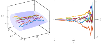
Figure 1: Realizations on the phase space (left) and relative control efforts (right). Control on the momentum.

Figure 2 highlights instead the trajectories of position (left) and momentum (right) with the corresponding confidence interval.

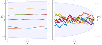
Figure 2: Position’s trajectories (left) and momentum’s trajectories (right). Control on the momentum.

In all the figures, the transparent blue tube represent the ”$3\sigma$” confidence interval, i.e. its intersection with the slice plane $t$ is given by

$$\left\{(q,p)\in{\mathbb{R}}^{2}\,\bigg{|}\,\begin{bmatrix}q&p\end{bmatrix}\Sigma_{t}^{-1}\begin{bmatrix}q\\ p\end{bmatrix}\leq 3^{2}\right\}.$$

The figures highlight the reduction of the variance of the momentum process as time increases to $T=1$.

References

- [1] K. J. Åström, Introduction to Stochastic Control Theorey, Academic Press, 1970.
- [2] Efstathios Bakolas, Finite-horizon covariance control for discrete-time stochastic linear systems subject to input constraints, Automatica, 91, pp. 61-68, 2018.
- [3] A. Beurling, An automorphism of product measures, Ann. Math. 72 (1960), 189-200.
- [4] A. Blaquière, “Controllability of a Fokker-Planck equation, the Schrödinger system, and a related stochastic optimal control (revised version),” Dynamics and Control, vol. 2, no. 3, pp. 235–253, 1992.
- [5] R. Brockett, “Notes on the control of the Liouville equation,” in Control of Partial Differential Equations. Springer, 2012, pp. 101–129.
- [6] Y. Chen, T.T. Georgiou and M. Pavon, “Optimal steering of a linear stochastic system to a final probability distribution, Part I”, IEEE Trans. Aut. Control, 61, Issue 5, 1158-1169, 2016.
- [7] Y. Chen, T.T. Georgiou and M. Pavon, “Optimal steering of a linear stochastic system to a final probability distribution, Part II”, IEEE Trans. Aut. Control, 61, Issue 5, 1170-1180, 2016.
- [8] Y. Chen, T.T. Georgiou and M. Pavon, “Fast cooling for a system of stochastic oscillators”, J. Math. Phys., 56, n.11, 113302, 2015.
- [9] Y. Chen, T.T. Georgiou and M. Pavon, On the relation between optimal transport and Schrödinger bridges: A stochastic control viewpoint, J. Optim. Theory and Applic., 169 (2), 671-691, 2016.
- [10] Y. Chen, T.T. Georgiou and M. Pavon, Optimal transport over a linear dynamical system, IEEE Trans. Aut. Control, 62, n. 5, 2137-2152, 2017.
- [11] T. M. Cover and J. A. Thomas, Elements of Information Theory, Wiley, New York, 1991.
- [12] P. Dai Pra, A stochastic control approach to reciprocal diffusion processes, Appl. Math. and Optimiz., 23 (1), 1991, 313-329.
- [13] P.Dai Pra and M.Pavon, On the Markov processes of Schroedinger, the Feynman-Kac formula and stochastic control, in Realization and Modeling in System Theory - Proc. 1989 MTNS Conf., M.A.Kaashoek, J.H. van Schuppen, A.C.M. Ran Eds., Birkäuser, Boston, 1990, 497- 504.
- [14] R. Filliger, M.-O. Hongler, and L. Streit, “Connection between an exactly solvable stochastic optimal control problem and a nonlinear reaction-diffusion equation,” Journal of Optimization Theory and Applications, vol. 137, no. 3, pp. 497–505, 2008.
- [15] H. Föllmer, Random fields and diffusion processes, in: Ècole d’Ètè de Probabilitès de Saint-Flour XV-XVII, edited by P. L. Hennequin, Lecture Notes in Mathematics, Springer-Verlag, New York, 1988, vol.1362,102-203.
- [16] R. Fortet, Résolution d’un système d’equations de M. Schrödinger, J. Math. Pure Appl. IX (1940), 83-105.
- [17] M. Goldshtein and P. Tsiotras, Finite-horizon covariance control of linear time-varying systems, in IEEE Conference on Decision andControl, Melbourne, Australia, Dec. 12-15, 2017, pp. 3606-3611.
- [18] K. M. Grigoriadis and R. E. Skelton, Minimum-energy covariance controllers, Automatica, 33, no. 4, pp. 569-578, 1997.
- [19] A. Halder and E. D. Wendel, Finite horizon linear quadratic Gaussian density regulator with Wasserstein terminal cost, in American Control Conference (ACC), 2016. IEEE, 2016, pp. 7249-7254.
- [20] A. Hotz and R. E. Skelton, Covariance control theory, International Journal of Control, 46, (1):13-32, 1987.
- [21] B. Jamison, The Markov processes of Schrödinger, Z.Wahrscheinlichkeitstheorie verw. Gebiete 32 (1975), 323-331.
- [22] C. Léonard, A survey of the Schroedinger problem and some of its connections with optimal transport, Discrete Contin. Dyn. Syst. A, 2014, 34 (4): 1533-1574.
- [23] A. Lindquist and G. Picci, Linear Stochastic Systems: A Geometric Approach to Modeling, Estimation and Identification, Springer, 2015.
- [24] T. Mikami, Monge’s problem with a quadratic cost by the zero-noise limit of h-path processes, Probab. Theory Relat. Fields, 129, (2004), 245-260.
- [25] T. Mikami and M. Thieullen, Duality theorem for the stochastic optimal control problem., Stoch. Proc. Appl., 116, 1815-1835 (2006).
- [26] T. Mikami and M. Thieullen, Optimal Transportation Problem by Stochastic Optimal Control, SIAM Journal of Control and Optimization, 47, N. 3, 1127-1139 (2008).
- [27] K. Okamoto and P. Tsiotras, Optimal Stochastic Vehicle Path Planning Using Covariance Steering, International Conference on Robotics and Automation, Montreal, Canada, May. 20?24, 2019.
- [28] M. Pavon and A. Wakolbinger, “On free energy, stochastic control, and Schrödinger processes,” in Modeling, Estimation and Control of Systems with Uncertainty. Springer, 1991, pp. 334–348.
- [29] M.Pavon, Stochastic control and non-Markovian Schrödinger processes,in Systems and Networks: Mathematical Theory and Applications, vol. II, U. Helmke, R.Mennichen and J.Saurer Eds., Mathematical Research vol.79, Akademie Verlag, Berlin, 1994, 409-412.
- [30] I. S. Sanov, On the probability of large deviations of random magnitudes (in Russian), Mat. Sb. N. S., 42 (84) (1957). Select. Transl. Math. Statist. Probab., 1, 213-244 (1961).
- [31] E. Schrödinger, Über die Umkehrung der Naturgesetze, Sitzungsberichte der Preuss Akad. Wissen. Berlin, Phys. Math. Klasse (1931), 144-153.
- [32] E. Schrödinger, Sur la théorie relativiste de l’électron et l’interpretation de la mécanique quantique, Ann. Inst. H. Poincaré 2, 269 (1932).
- [33] R. Sinkhorn, A relationship between arbitrary positive matrices and doubly stochastic matrices, Ann. Math. Statist., 35 (1964), 876-879.
- [34] C. Villani, Topics in optimal transportation, AMS, 2003, vol. 58.
- [35] A. Wakolbinger, Schrödinger Bridges from 1931 to 1991, in: E. Cabaa et al. (eds) , Proc. of the 4th Latin American Congress in Probability and Mathematical Statistics, Mexico City 1990, Contribuciones en probabilidad y estadistica matematica 3 (1992) , 61-79.