Solvable model for quantum criticality between Sachdev-Ye-Kitaev liquid and disordered Fermi liquid

Abstract

We propose a simple solvable variant of the Sachdev-Ye-Kitaev (SYK) model which displays a quantum phase transition from a fast-scrambling non-Fermi liquid to disordered Fermi liquid. Like the canonical SYK model, our variant involves a single species of Majorana fermions connected by all-to-all random four-fermion interactions. The phase transition is driven by a random two-fermion term added to the Hamiltonian whose structure is inspired by proposed solid-state realizations of the SYK model. Analytic expressions for the saddle point solutions at large number $N$ of fermions are obtained and show a characteristic scale-invariant $\sim|\omega|^{-1/2}$ behavior of the spectral function below the transition which is replaced by a $\sim|\omega|^{-1/3}$ singularity exactly at the critical point. These results are confirmed by numerical solutions of the saddle point equations and discussed in the broader context of the field.

I Introduction

Sachdev-Ye-Kitaev modelSachdev and Ye (1993); Kitaev (2015) is an exactly solvable model of a non-Fermi liquid connected to quantum gravity theories through the holographic principleSachdev (2015); Maldacena and Stanford (2016). The SYK model and its variants Polchinski and Rosenhaus (2016); Fu et al. (2017); Witten (2016); Banerjee and Altman (2017); Berkooz et al. (2017); Bi et al. (2017); Murugan et al. (2017); Peng et al. (2017); Lantagne-Hurtubise et al. (2018) show intriguing behaviors as well as unexpected relations to seemingly unrelated areas of physics, ranging from strongly correlated fermionsLiu et al. (2018); Song et al. (2017); Huang and Gu (2017); Jian et al. (2017); Wu et al. (2018) to quantum chaos,Hosur et al. (2016); Gu et al. (2017); Chen et al. (2017); Krishnan et al. (2017) quantum information theory,García-Álvarez et al. (2017); Luo et al. (2017) random matrix theoryYou et al. (2017); García-García and Verbaarschot (2016); Li et al. (2017), many-body localizationJian and Yao (2017) and wormhole dynamics.Maldacena and Qi (2018) Several proposals for experimental realizations of the SYK model have been givenDanshita et al. (2017); Pikulin and Franz (2017); Chew et al. (2017); Chen et al. (2018) which raises prospects for testing these ideas in a laboratory.

The standard SYK model is controlled by a single dimensionless parameter (the strength of interactions $J$ divided by temperature $T$) and remains in the same phase for all its values. An interesting class of models seeks to modify the SYK Hamiltonian such that it undergoes a transition to another phase by tuning a control parameter. Banerjee and AltmanBanerjee and Altman (2017) introduced an SYK model with coupling to a set of “auxiliary fermions” which exhibits a quantum phase transition from the non-Fermi liquid SYK phase to a disordered Fermi liquid as the ratio of the number of SYK fermions to the number of auxiliary fermions is tuned. Bi et al. Bi et al. (2017) considered a model with modified structure of four-fermion coupling constants which likewise undergoes a phase transition out of the SYK liquid as a dimensionless parameter characterizing this structure is tuned. These studies are inherently important because they elucidate the limits of stability of the SYK liquid and show how it relates to other more conventional quantum phases of interacting fermions. Understanding these relations is clearly essential for all future attempts to experimentally realize the SYK model.

In this work we propose an extension of the SYK model achieved by including a random bilinear term in the Hamiltonian, whose structure is inspired by experimental considerations Lantagne-Hurtubise et al. (2018). This additional term leads to a tunable non-Fermi liquid to Fermi liquid (nFL/FL) transition similar in some ways to the one seen in Banerjee-Altman model Banerjee and Altman (2017). The advantage of our model is that it is possible to observe such a transition without introducing an additional flavor of fermions. In addition, the scaling form of the spectral function can be obtained analytically for the model directly at the critical point.

In the following we define our model and discuss the physics that drives the nFL/FL phase transition. We then obtain the saddle point equations for the fermion propagator in the limit of large number $N$ of fermions and analytically extract the low-energy scaling behavior on both sides of the phase transition and at the critical point. We numerically solve the saddle point equations and confirm the validity of the low-energy scaling forms obtained analytically.

II Model

We extend the canonical SYK model Kitaev (2015) for $N$ Majorana fermions by introducing a random bilinear term as follows

$$H=\sum_{i<j}K_{ij}\chi_{i}\chi_{j}+\sum_{i<j<k<l}J_{ijkl}\chi_{i}\chi_{j}\chi_{k}\chi_{l}.$$ (1)

Here $J_{ijkl}$ denote real coupling constants drawn from a Gaussian random distribution with $\overline{J_{ijkl}}=0$ and $\overline{J^{2}_{ijkl}}=3!J^{2}/N^{3}$. The form of the bilinear coupling $K_{ij}$ is inspired by proposed experimental realizations of the SYK model in solid-state systemsPikulin and Franz (2017); Chew et al. (2017); Chen et al. (2018) where the randomness in $J_{ijkl}$ and $K_{ij}$ arises from the disordered spatial structure of the single-particle wavefunctions of the zero modes which comprise the active Majorana degrees of freedom. Following Ref. Lantagne-Hurtubise et al., 2018 we take

$$K_{ij}=-i\mu\sum_{m=1}^{2M}(a_{i}^{m}b_{j}^{m}-b_{i}^{m}a_{j}^{m})$$ (2)

where $a_{i}^{m},b_{j}^{m}$ are random Gaussian independent variables such that $\overline{a_{i}^{m}}=\overline{b_{i}^{m}}=0$ and $\overline{a_{i}^{m}a_{j}^{n}}=\overline{b_{i}^{m}b_{j}^{n}}=\frac{1}{8M}\delta_{ij}\delta^{mn}$ as well as $\overline{a_{i}^{m}b_{j}^{n}}=0$ which implies $K^{2}=N\overline{K^{2}_{ij}}=\mu^{2}/16p$ if we define

$$p=M/N.$$ (3)

In the above overline denotes the average over Gaussian distribution.

As noted in Ref. Lantagne-Hurtubise et al., 2018 model defined by Eq. (1) exhibits a phase transition already at the non-interacting level (i.e. when $J=0$). In this case the single-particle energy spectrum is given by the eigenvalues of the hermitian matrix $K_{ij}$ defined in Eq. (2). The key observation is that quantities $a^{m}$ and $b^{m}$ can be viewed as $N$-component vectors in index $i$ and are, for large $N$, approximately orthogonal to each other. As a result, the rank of the matrix $K_{ij}$ is close to $4M$. When $4M<N$ the matrix is rank-deficient and, as a result, has $(N-4M)$ zero modes. One can further demonstrateLantagne-Hurtubise et al. (2018) that its other eigenvalues cluster around $\pm\mu/8p$. For $p<p_{c}={1/4}$ the zero-mode manifold is separated from the rest of the spectrum by a gap $\Delta$. When interactions are turned on for $p<p_{c}$ one might expect that they transform the degenerate manifold of states at zero energy into an SYK liquid. This is intuitively clear for weak interactions $J\ll\Delta$ where one can focus on the zero modes and note that the low energy theory becomes a canonical SYK model for $(N-4M)$ Majorana fermions in the zero-mode manifold. As $p$ approaches $p_{c}$ the gap closes and the intuitive argument given above fails. In the opposite limit, $p\gg p_{c}$, the matrix elements $K_{ij}$ become Gaussian-distributed by virtue of the central limit theorem. The non-interacting phase is then a disordered gapless Fermi liquid with a semicircle spectral density. In this limit it is easy to show that interactions constitute an irrelevant perturbation. One therefore expects a phase transition, as a function of increasing parameter $p$, from the SYK liquid to disordered Fermi liquid in this model.

The model defined by Eqs. (1) and (2) can be solved, in the large-$N$ limit, by the saddle-point expansion technique developed for the original SYK model.Sachdev (2015); Maldacena and Stanford (2016) Averaging over random variables $a_{i}^{m},b_{j}^{m}$ that enter the definition of $K_{ij}$ involves an extra step that has been described in Ref. Lantagne-Hurtubise et al., 2018. That study however considered only the non-interacting model. Here we give the solution for the full interacting model. Details fo the calculation are outlined in Appendix A. The resulting Matsubara frequency Schwinger-Dyson equation for the fermion propagator $G(\tau)=\frac{1}{N}\sum_{i}\langle\hat{T}\chi_{i}(\tau)\chi_{i}(0)\rangle$ reads

$$G^{-1}(i\omega_{n})=-i\omega_{n}-\Sigma(i\omega_{n})$$ (4)

where the self-energy is given by

$$\Sigma(i\omega_{n})=\Sigma_{J}(i\omega_{n})+4pK^{2}\frac{G(i\omega_{n})}{4p-K^{2}G(i\omega_{n})^{2}}.$$ (5)

The interaction part of the self energy

$$\Sigma_{J}(\tau)=J^{2}G(\tau)^{3}$$ (6)

is the same as in the original Majorana SYK model.

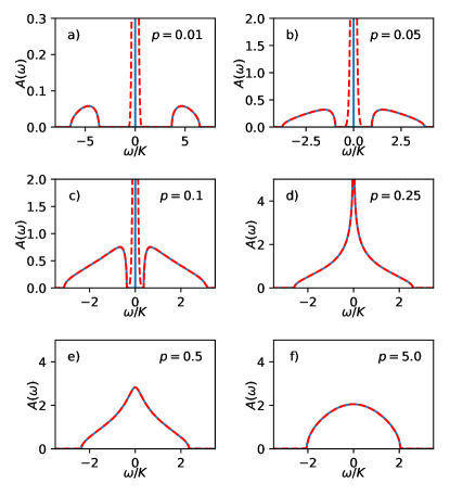
Figure 1: Evolution of the spectral function $A(\omega)$ across the quantum phase transition tuned by parameter $p=M/N$. Spectral functions are computed by a numerical iteration of the large-$N$ saddle-point equations in Keldysh representation given in Appendix B. Results for non-interacting ($J=0$, blue solid line) and interacting ($J=K$, red dashed line) cases are overlaid for each $p$. Note that the interactions broaden the zero modes inside the gap for $p<1/4$, resulting in a SYK non-Fermi liquid. Above the transition for $p>1/4$, interactions are irrelevant and do not significantly modify the spectral function.

III Properties of the model

III.1 The non-interacting case

We briefly summarize the properties of the non-interacting model. The non-interacting problem, obtained by taking $J=0$ in Eq. (6), has a simple solution Lantagne-Hurtubise et al. (2018) in the large-$N$ limit. Dropping $\Sigma_{J}$ equations (4) and (5) can be combined into a single cubic equation for the propagator in the frequency domain

$$i\omega K^{2}G^{3}+(1-4p)K^{2}G^{2}-4ip\omega G-4p=0.$$ (7)

For $p<1/4$, the energy spectrum has a gap with a degenerate manifold of zero modes. Contribution of these zero modes to the spectral density is given by $\rho(\omega)=(1-4p)\delta(\omega)$. As $p$ increases, the gap gradually closes until a phase transition occurs at $p=p_{c}=1/4$. At the transition the spectral function shows the $A(\omega)\sim\omega^{-1/3}$ scaling. For $p>1/4$ the spectrum remains gapless and approaches the semicircle distribution for large $p$.

While the Matsubara formalism is useful for analytical calculations we turn to the Keldysh technique, formulated directly in the real time domain, to obtain numerical solutions of the large-$N$ saddle point equations. It allows us to easily extract the spectral function (without the need to analytically continue from imaginary time) and the numerical solution converges rapidly which is important when interactions are included. In the Keldysh picture propagator $G$ becomes at $2\times 2$ matrix with elements $G_{ss^{\prime}}$ where $s$ represents the contour index for forward and backward paths on the Keldysh contour. Appendix B gives a brief summary of the technique applied to the SYK model while a detailed discussion of the Keldysh formalism can be found in Ref. Kamenev and Levchenko, 2009. The Keldysh version of the above cubic equation (7) reads

$$-\omega K^{2}(\sigma^{z}G)^{3}+K^{2}(1-4p)(\sigma^{z}G)^{2}\\ +4p\omega\sigma^{z}G-4p=0,$$ (8)

where $\sigma^{z}$ acts in the $s$-$s^{\prime}$ space. Once the solution is obtained, matrix $G$ contains $G^{T}$,$G^{<}$,$G^{\hat{T}}$ and $G^{>}$ as its elements. The retarded Green’s function can then be obtained as $G^{R}(\omega)=G^{T}(\omega)-G^{<}(\omega)$ which allows us to compute the spectral function $A(\omega)=-2\text{Im}G_{R}(\omega)$. Fig. 1 shows numerical solutions of Eq. (8) for different values of parameter $p$. These agree with the discussion given below Eq. (7).

III.2 Interacting regime

We observed a degenerate manifold of zero modes in the non-interacting regime for $p<p_{c}$ separated by a gap from the rest of the spectrum. For weak interaction strength $J$ we can focus on the zero-mode manifold and disregard the rest of the spectrum. The effective low-energy model is then simply an SYK Hamiltonian for the Majorana modes comprising the zero-mode manifold. We thus expect the $\delta$-function in the spectral density to broaden due to interactions and form a low-energy SYK liquid. Above the non-interacting transition point ($p>p_{c}$) the single-particle spectrum is gapless. In this case weak four-fermion interactions are known to be irrelevant and we thus expect the interacting system to form a disordered Fermi liquid in this regime.

In the two limits discussed above and at the transition ($p=p_{c}$) it is possible to analytically extract the low energy scaling behavior of the fermion propagator from Eqs. (4-6). In the following, we show that these results indeed confirm the expectations based on the general arguments presented above and we further support these findings by full numerical solutions of the large-$N$ saddle point equations in Keldysh picture.

III.2.1 Scaling behavior at the transition, $p=p_{c}=1/4$

For $p=1/4$, where we observed the transition for the non-interacting system, Eqs. (4) and (5) reduce to

$$-i\omega-\Sigma_{J}(i\omega)+\frac{1}{G(i\omega)}\left({1-\frac{1}{K^{2}G^{2}(i\omega)}}\right)^{-1}=\frac{1}{G(i\omega)}$$ (9)

In order to obtain the scaling form of $G(i\omega)$, we make a power law ansatz of the form

$$G(i\omega)\sim\omega^{-\alpha}.$$ (10)

For $\alpha>0$ we can always go to sufficiently low frequency that $|G|\gg 1/K$ holds. We can then expand the denominator to first order in $1/(KG)^{2}$ and obtain

$$i\omega\simeq\frac{1}{K^{2}G^{3}(i\omega)}-\Sigma_{J}(i\omega)$$ (11)

Given the power law ansatz (10), we would like to extract the scaling form of the SYK self energy defined in Eq. (6). To this end we write the Fourier transform $G(\tau)=\int d\omega e^{-i\omega\tau}G(i\omega)$. Using a simple result

$$\int d\omega e^{-i\omega\tau}\omega^{-\alpha}\sim\tau^{(\alpha-1)}$$ (12)

we find that the frequency dependence assumed in Eq. (10) transforms to $G(\tau)\sim\tau^{(\alpha-1)}$. Eq. (6) then implies $\Sigma_{J}(\tau)\sim\tau^{3(\alpha-1)}$ and the inverse Fourier transform finally leads to $\Sigma_{J}(i\omega)\sim\omega^{2-3\alpha}$. We can now rewrite Eq. (11) as

$$\omega\simeq A\omega^{3\alpha}+B\omega^{2-3\alpha}$$ (13)

where we absorbed all prefactors into constants $A$ and $B$. This equation has a solution for $\alpha=1/3$. Therefore, at $p=p_{c}$ we expect $G\sim\omega^{-1/3}$. Remarkably, at the critical point, the scaling form of the propagator is unchanged by the interactions even though $\Sigma_{J}$ enters with the same power in Eq. (13) as the non-interacting contribution. Interactions are exactly marginal at the non-interacting critical point.

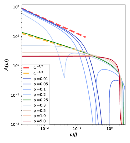
Figure 2: Low-frequency scaling behavior of the spectral function $A(\omega)$ for various values of $p$. Other parameters $K=J$ and $T=0.0003J$ are fixed. Analytically obtained scaling forms are shown by dashed lines. For $p<1/4$ spectral function tends to $A(\omega)\sim\omega^{-1/2}$, characteristic of the SYK model. At the nFL/FL transition (green) where $p=1/4$ we confirm that $A(\omega)\sim\omega^{-1/3}$ in accord with the prediction. Above the transition $A(\omega)$ tends to a frequency-independent constant as expected for disordered Fermi liquid.

III.2.2 Deep in non-Fermi liquid phase, $p\ll p_{c}$

We expect the zero modes to broaden into an SYK peak with $G\sim|\omega|^{-1/2}$ when $p\ll p_{c}$. In order to see this, we note that in the low-frequency limit we can neglect $p$ in the denominator of Eq. (5) which then reduces to

$$\Sigma(i\omega)\simeq\Sigma_{J}(i\omega)-4p\frac{1}{G(i\omega)}.$$ (14)

If we take $J=0$ for a moment, we observe that the expression above combined with Dyson’s equation (4) simplify to

$$G(i\omega)=-\frac{1-4p}{i\omega}.$$ (15)

which gives the spectral density $\rho(\omega)=(1-4p)\delta(\omega)$ after analytic continuation. This is the degenerate manifold of zero modes expected in the absence of interactions.

Now we turn on the interactions ($J>0$) and investigate how $\Sigma_{J}$ scales for low frequencies given Eq. (15). We find that $G(\tau)\sim\tau^{0}$ for $\tau\rightarrow\infty$ which implies that $\Sigma_{J}(\tau)\sim\tau^{0}$ as $\tau\rightarrow\infty$. We can compare this to the second term $\Sigma_{K}(i\omega)=-4p/G(i\omega)$ in Eq. (14) which is the contribution to the self energy $\Sigma$ due to the bilinear term in Hamiltonian (1). The latter scales as $\Sigma_{K}(\tau)\sim\tau^{-2}$, and is therefore dominated by $\Sigma_{J}\sim\tau^{0}$ at long times. We therefore conclude that interactions are relevant and the manifold of zero modes turns into an SYK liquid where the low energy solution, characterized by the inverse square root singularity, is well known Kitaev (2015); Sachdev (2015).

III.2.3 Deep in disordered Fermi liquid phase, $p\gg p_{c}$

For large $p\gg p_{c}$, the self energy in Eq. (5) reduces to

$$\Sigma(i\omega)\simeq\Sigma_{J}(i\omega)+K^{2}G(i\omega)$$ (16)

If we take $J=0$ and ignore $\Sigma_{J}$, the exact solution is available Pikulin and Franz (2017) for it becomes a simple quadratic equation in $G(i\omega)$ and the low energy limit of the solution is given by $G(i\omega)=i\text{sgn(}\omega\text{)}/K$. This implies $G(\tau)\sim 1/\tau$ for $\tau\rightarrow\infty$. As we turn on interactions, we find $\Sigma_{J}(\tau)=J^{2}G^{3}(\tau)\sim 1/\tau^{3}$ which implies $\Sigma_{J}(i\omega)\sim\omega^{2}$, irrelevant at low frequencies compared to the second term in Eq. (16). We conclude that for large $p$ the bilinear term dominates and the spectral function becomes a semicircle characteristic of disordered Fermi liquid shown in Fig. 1f. Interactions have no significant effect in this limit.

III.3 Numerical results

To confirm the approximate analytical results given above and to extend them beyond the low-frequency regime we solve the Keldysh version of the large-$N$ saddle point equations (4-6) by numerical iteration. The Keldysh saddle point equations are derived in Appendix B and the details of our numerical procedure are described in Appendix C. Fig. 1 shows the numerically calculated spectral functions for various values of parameter $p$ over the full range of frequencies while Fig. 2 focuses on the low-frequency scaling limit. These results are in excellent agreement with analytical scaling forms derived in the preceding subsection and confirm that the phase transition survives the inclusion of strong interactions which transform the gapped phase with degenerate ground state manifold into the SYK non-Fermi liquid.

IV Summary and conclusions

We proposed an extension of the Sachdev-Ye-Kitaev model which exhibits a quantum phase transition from a non-Fermi liquid state to a disordered Fermi liquid tuned by a dimensionless parameter $p$ which, in essence, controls the rank of the hermitian matrix in the part of the Hamiltonian that is bi-linear in fermion operators. The large-$N$ saddle point equations for the model can be solved analytically in three limiting cases which establishes the existence of two distinct stable phases in the model as well as the scale-invariant behavior at the critical point. These conclusions are confirmed in detail by numerical solutions of the Keldysh version of the saddle point equations.

The nFL phase that occurs for $p<p_{c}$ has an effective description as a canonical SYK model with $N(1-p/p_{c})$ fermions separated by a gap from the rest of the spectrum. Although we have not computed the out-of-time order correlator for the model we expect the nFL phase to saturate the upper bound on the Lyapunov exponent $\lambda\leq 2\pi T$ just like the Banerjee-Altman modelBanerjee and Altman (2017). The $p<p_{c}$ phase is therefore expected to be a fast-scrambling, maximally chaotic nFL. Above the transition we found interactions to be irrelevant and therefore expect this phase to be slow-scrambling, non-chaotic Fermi liquid. For $p\gg p_{c}$ case (Eq.16) it has been shown García-García et al. (2018) that $\lambda<2\pi T$ does not saturate the chaos bound and vanishes below a critical temperature $T^{*}$. The model, therefore, shows a phase transition from fast to slow scrambling dynamics in what is perhaps the simplest possible setting.

Several extensions of our model are possible and potentially interesting. The model can be formulated in higher dimensions by coupling islands described by Hamiltonian (1) via four-fermion couplings as in Ref. Gu et al., 2017. Such a system is then expected to show quantum chaos propagation with a characteristic “butterfly velocity” in its chaotic phase and exhibit a transition to non-chaotic phase as $p$ exceeds the critical value. Another obvious extension is to formulate the model with complex fermions as in Refs. Sachdev, 2015; Banerjee and Altman, 2017. Complex-fermion SYK model exhibits richer behavior because it permits the addition of the chemical potential term to control fermion density. The phase transition observed in the Majorana version of the model studied in this work could show further interesting behavior as a function of density.

APPENDIX

IV.1 Large-$N$ solution via imaginary-time path integral

We follow the standard procedure outlined in Ref. Maldacena and Stanford, 2016, the so called $G$-$\Sigma$ formalism, which leads to saddle point equations for the fermion propagator and the self energy that become asymptotically exact in the limit of large number of fermions $N$. As the first step we reformulate the problem defined by Hamiltonian (1) as an imaginary time path integral for the partition function $Z=\int\mathcal{D}[\chi]e^{-S}$ where the action reads

$$S[\chi]=\int d\tau\left[\frac{1}{2}\sum_{i}\chi_{i}\partial\chi_{i}-i\mu\sum_{ijm}a_{i}^{m}b_{j}^{m}\chi_{i}\chi_{j}+\sum_{ijkl}J_{ijkl}\chi_{i}\chi_{j}\chi_{k}\chi_{l}\right].$$ (17)

To decouple the random variables $a^{m}_{i}$ and $b^{m}_{j}$ we employ the identity $\int\mathcal{D}[\psi_{a},\psi_{b}]\exp\left(-i\mu\int d\tau\sum_{m}\psi^{m}_{a}\psi^{m}_{b}\right)=1$ where $\psi^{m}_{a}$ and $\psi^{m}_{b}$ are auxiliary Grassman variables. After change of variables $\psi_{a}^{m}\rightarrow\psi_{a}^{m}+\sum_{i}a_{i}^{m}\chi_{i}$ and $\psi_{b}^{m}\rightarrow\psi_{b}^{m}+\sum_{j}b_{j}^{m}\chi_{j}$ we obtain

$$S[\psi_{a},\psi_{b},\chi]=\int d\tau\left[\frac{1}{2}\chi_{i}\partial_{\tau}\chi_{i}+i\mu\left(\psi_{a}^{m}\psi_{b}^{m}-a_{i}^{m}\psi_{b}^{m}\chi_{i}+b_{j}^{m}\psi_{a}^{m}\chi_{j}\right)+\sum_{ijkl}J_{ijkl}\chi_{i}\chi_{j}\chi_{k}\chi_{l}\right].$$ (18)

It is now straightforward to perform the Gaussian average over the random variables which leads to an action that is bi-local in time variable

$$S=\int d\tau\left[\frac{1}{2}\sum_{i}\chi_{i}\partial_{\tau}\chi_{i}+i\mu\sum_{m}\psi^{m}_{a}\psi^{m}_{b}\right]-\frac{K^{2}}{N}\int d\tau d\tau^{\prime}\left[\sum_{m}\psi_{b}^{m}(\tau)\psi_{b}^{m}(\tau^{\prime})\sum_{i}\chi_{i}(\tau)\chi_{i}(\tau^{\prime})\right]+(a\leftrightarrow b)\\ -\frac{J^{2}}{8N^{3}}\int d\tau d\tau^{\prime}\left(\sum_{i}\chi_{i}(\tau)\chi_{i}(\tau^{\prime})\right)^{4}.$$

More details on the steps above can be found in Ref. Lantagne-Hurtubise et al., 2018. We next introduce propagators for fermionic degrees of freedom using bosonic path integral identities $\int\mathcal{D}[\Sigma]\exp\left(-\frac{N}{2}\Sigma(\tau,\tau^{\prime})\left[G(\tau,\tau^{\prime})-\frac{1}{N}\sum_{i}\chi_{i}(\tau)\chi(\tau^{\prime})\right]\right)=1$ and $\int\mathcal{D}[\Omega]\exp\left(-M\Omega^{\alpha\beta}(\tau,\tau^{\prime})\left[F^{\beta\alpha}(\tau,\tau^{\prime})-\frac{1}{2M}\sum_{m}\psi^{m}_{\alpha}(\tau)\psi_{\beta}^{m}(\tau^{\prime})\right]\right)=1$ where $\Sigma$ and $\Omega$ act as Lagrange multipliers and have physical interpretation as fermion self energies. After integrating out fermions we obtain the saddle-point action

$$S=\frac{N}{2}\text{tr}\log\left[-\partial_{\tau}+\Sigma\right]+M\text{tr}\log\left[\mu\sigma^{y}+\Omega\right]+\int d\tau d\tau^{\prime}\left[\frac{N}{2}\Sigma G+M\Omega^{\alpha\beta}F^{\beta\alpha}+2K^{2}M(F^{aa}+F^{bb})G-\frac{J^{2}}{8}NG^{4}\right]$$ (19)

where we suppressed temporal dependence for the sake of brevity. Indices $\alpha,\beta$ take values $a,b$ and summation over repeated indices is assumed. We note that except for the last term, which incorporates the effect of interactions, the action (19) has the same form as the action derived in Appendix A of Ref. Lantagne-Hurtubise et al., 2018.

Varying the action with respect to the self energies gives the two Dyson equations,

$$G(i\omega_{n})(i\omega_{n}-\Sigma(i\omega_{n}))=1$$ (20)

$$\sum_{\gamma}F^{\alpha\gamma}(i\omega)\left(\mu\sigma^{y}_{\gamma\beta}+\Omega^{\gamma\beta}(i\omega)\right)=-\delta^{\alpha\beta}.$$ (21)

Varying with respect to the propagators yields the saddle-point equations for self energies,

$$\Sigma(\tau,\tau^{\prime})=J^{2}G(\tau,\tau^{\prime})^{3}-4pK^{2}F^{\gamma\gamma}(\tau,\tau^{\prime})$$ (22)

$$\Omega^{\alpha\beta}(i\omega)=-2K^{2}\delta^{\alpha\beta}G(i\omega).$$ (23)

Notice that $\Omega^{\alpha\beta}=\Omega\delta_{\alpha\beta}$ is diagonal according to Eq. (23) where we defined $\Omega=-2K^{2}G$. This ensures that $F^{aa}=F^{bb}\equiv F$ which can be seen by explicitly writing (21) as a matrix product. Then equation (21) can be simplified to

$$F(\mu^{2}-\Omega^{2})=\Omega$$ (24)

which can be seen by explicitly writing out the matrix product. Substituting $\Omega=-2K^{2}G$ we then obtain

$$F=-\frac{G}{2(4p-K^{2}G^{2})}.$$ (25)

Finally substituting this into Eq. (22) (notice the repeated indices) we obtain the self-energy expression (5) to be solved in combination with equation (20). Note that from (22) we defined $\Sigma_{J}(\tau,\tau^{\prime})=J^{2}G(\tau,\tau^{\prime})^{3}$.

IV.2 Keldysh Path Integral

To derive the Keldysh version of large-$N$ saddle point equations we follow Ref. Song et al., 2017. (For an introduction to Keldysh formalism see e.g. Ref. Kamenev and Levchenko, 2009). We write down the Keldysh path integral for Hamiltonian (1) and disorder-average the partition fuction $Z$ over Gaussian random variables of the model. This process is almost identical to the disorder averaging of SYK models in Matsubara formalism Maldacena and Stanford (2016). The non-standard form of the bilinear coupling $K_{ij}$ is handled in a fashion nearly identical to Appendix A above. Disorder averaged Keldysh path integral is given by

$$\overline{Z}=\int\mathcal{D}\left[\chi,\psi\right]e^{iS},$$ (26)

where the action reads

$$iS=\frac{i}{2}\int d\tau\sum_{i}\chi_{i}\partial_{\tau}\chi_{i}-\mu\int d\tau\sum_{m}\psi_{a}^{m}\psi_{b}^{m}-\frac{J^{2}}{8N^{3}}\int d\tau_{1}d\tau_{2}\left(\sum_{i}\chi_{i}(\tau_{1})\chi_{i}(\tau_{2})\right)^{4}\\ +\frac{K^{2}}{N}\sum_{\alpha}\int d\tau_{1}d\tau_{2}\left(\sum_{m}\psi^{m}_{\alpha}(\tau_{1})\psi^{m}_{\alpha}(\tau_{2})\right)\left(\sum_{i}\chi_{i}(\tau_{2})\chi_{i}(\tau_{1})\right).$$ (27)

Writing the contour integral $\int d\tau$ in terms of forward and backward real time branches we find

$$iS=\sum_{ss^{\prime}}\int dtdt^{\prime}\Bigg{\{}\frac{i}{2}\sum_{i}\chi^{i}_{st}[\sigma^{z}_{ss^{\prime}}\delta_{tt^{\prime}}i\partial_{t}]\chi^{i}_{s^{\prime}t^{\prime}}-\mu\sigma^{z}_{ss^{\prime}}\sum_{m}\delta_{tt^{\prime}}\psi_{ast}^{m}\psi_{bs^{\prime}t^{\prime}}^{m}\\ +ss^{\prime}\frac{K^{2}}{N}\sum_{\alpha}\left(\sum_{m}\psi^{m}_{\alpha st}\psi^{m}_{\alpha s^{\prime}t^{\prime}}\right)\left(\sum_{i}\chi^{i}_{s^{\prime}t^{\prime}}\chi^{i}_{st}\right)-ss^{\prime}\frac{J^{2}}{8N^{3}}\left(\sum_{i}\chi_{ist}\chi_{is^{\prime}t^{\prime}}\right)^{4}\\ +\frac{N}{2}\Sigma_{ss^{\prime}}^{tt^{\prime}}\left(G_{s^{\prime}s}^{t^{\prime}t}-\frac{i}{N}\sum_{i}\chi^{i}_{st}\chi^{i}_{s^{\prime}t^{\prime}}\right)+M(\Omega^{\alpha\beta})_{ss^{\prime}}^{tt^{\prime}}\left((F_{\beta\alpha})_{s^{\prime}s}^{t^{\prime}t}-\frac{i}{2M}\sum_{m}\psi^{m}_{\alpha st}\psi^{m}_{\beta s^{\prime}t^{\prime}}\right)\Bigg{\}}$$ (28)

where we introduced bosonic path integral identities $\int\mathcal{D}[G,\Sigma]\exp{\left(\frac{N}{2}\sum_{ss^{\prime}}\int\int dtdt^{\prime}\Sigma^{tt^{\prime}}_{ss^{\prime}}\left[G_{s^{\prime}s}^{t^{\prime}t}-\frac{i}{N}\sum_{i}\chi^{i}_{st}\chi^{i}_{s^{\prime}t^{\prime}}\right]\right)}=1$ and $\int\mathcal{D}[\mathcal{G},\Omega]\exp{\left(M\sum_{ss^{\prime}}\int\int dtdt^{\prime}(\Omega^{\alpha\beta})_{ss^{\prime}}^{tt^{\prime}}\left[(F_{\beta\alpha})_{s^{\prime}s}^{t^{\prime}t}-\frac{i}{2M}\sum_{m}\psi^{m}_{\alpha st}\psi^{m}_{\beta s^{\prime}t^{\prime}}\right]\right)}=1$. As in the Matsubara case, $\Sigma$ and $\Omega$ act as Lagrange multipliers and can be though of as self energies. Gaussian integration over the fermionic degrees of freedom yields

$$iS=\frac{N}{2}\text{tr}\log A+M\text{tr}\log B\\ +\sum_{ss^{\prime}}\int dtdt^{\prime}\left\{\frac{N}{2}\Sigma_{ss^{\prime}}^{tt^{\prime}}G_{s^{\prime}s}^{t^{\prime}t}+M[\Omega^{\alpha\beta}]_{ss^{\prime}}^{tt^{\prime}}[F_{\beta\alpha}]_{s^{\prime}s}^{t^{\prime}t}-\frac{J^{2}}{8}ss^{\prime}N(G_{s^{\prime}s}^{t^{\prime}t})^{4}+2K^{2}Mss^{\prime}[F_{\alpha\alpha}]_{s^{\prime}s}^{t^{\prime}t}G_{ss^{\prime}}^{tt^{\prime}}\right\}$$

where we defined

$$A_{st,s^{\prime}t^{\prime}} =-i^{2}\left(\sigma^{z}_{ss^{\prime}}\delta(t-t^{\prime})i\partial_{t}-\Sigma_{ss^{\prime}}^{tt^{\prime}}\right)$$ (29)

$$B_{\alpha st,\beta s^{\prime}t^{\prime}} =i\left([\Omega^{\alpha\beta}]_{ss^{\prime}}^{tt^{\prime}}+\mu\sigma^{z}_{ss^{\prime}}\sigma^{y}_{\alpha\beta}\delta(t-t^{\prime})\right).$$ (30)

The saddle point equations are obtained after following functional derivatives and Fourier transforms

$$\frac{\delta S}{\delta\Sigma_{s_{1}s_{2}}^{t_{1}t_{2}}}=0,\hskip 20.0pt\frac{\delta S}{\delta[\Omega^{\alpha\beta}]_{s_{1}s_{2}}^{t_{1}t_{2}}}=0,$$ (31)

$$\frac{\delta S}{\delta G_{s_{1}s_{2}}^{t_{1}t_{2}}}=0,\hskip 20.0pt\frac{\delta S}{\delta[F_{\alpha\beta}]_{s_{1}s_{2}}^{t_{1}t_{2}}}=0.$$ (32)

The following then must be valid at saddle point

$$\sum_{s_{1},\gamma}F^{\alpha\gamma}_{ss_{1}}(\omega)\left(\Omega^{\gamma\beta}_{s_{1}s^{\prime}}(\omega)+\mu\sigma^{z}_{s_{1}s^{\prime}}\sigma^{y}_{\gamma\beta}\right)+\delta_{\alpha\beta}^{ss^{\prime}} =0$$ (33)

$$G_{ss_{1}}(\omega)(\omega\sigma_{s_{1}s^{\prime}}^{z}-\Sigma_{s_{1}s^{\prime}}(\omega)) =\delta_{ss^{\prime}}$$ (34)

$$\frac{1}{2}\Sigma_{ss^{\prime}}^{tt^{\prime}}-\frac{J^{2}}{2}ss^{\prime}(G_{s^{\prime}s}^{t^{\prime}t})^{3}+2K^{2}\frac{M}{N}ss^{\prime}[F_{\alpha\alpha}]_{ss^{\prime}}^{tt^{\prime}} =0$$ (35)

$$[\Omega^{\alpha\beta}]_{ss^{\prime}}^{tt^{\prime}}+2K^{2}ss^{\prime}G_{ss^{\prime}}^{tt^{\prime}}\delta_{\alpha\beta} =0$$ (36)

Equation (36) tells us that $\Omega^{\alpha\beta}_{ss^{\prime}}=\delta^{\alpha\beta}\Omega_{ss^{\prime}}$ is diagonal. It follows that $F=F^{aa}=F^{bb}$, similar to Matsubara case in Appendix A. Equation (33) can then be recast as

$$F(\mu^{2}-\Omega\sigma^{z}\Omega\sigma^{z})=\sigma^{z}\Omega\sigma^{z}$$ (37)

where $F$, $\Omega$, $\sigma^{z}$ are now matrices in Keldysh forward-backward indices. In this matrix language, we similarly see that equations (34-36) become

$$G(\omega\sigma^{z}-\Sigma)=I$$ (38)

$$\Sigma=\Sigma_{J}-8K^{2}p\sigma^{z}F\sigma^{z},$$ (39)

$$\Omega+2K^{2}\sigma^{z}G\sigma^{z}=0,$$ (40)

where $[\Sigma_{J}(t-t^{\prime})]_{ss^{\prime}}=J^{2}ss^{\prime}(G_{s^{\prime}s}^{t^{\prime}t})^{3}$ and $p=M/N$. Eliminating $\Omega$ and $F$ by combining equations (37-40) we obtain the simplified saddle point equations

$$\Sigma=4pK^{2}\sigma^{z}G[\sigma^{z}(4p-K^{2}(\sigma^{z}G)^{2})]^{-1}+\Sigma_{J},$$ (41)

$$G=(\omega\sigma^{z}-\Sigma)^{-1}.$$ (42)

For the non-interacting case $J=0$, we set $\Sigma_{J}=0$ and combine these two equations to obtain equation (8). Since we are interested in the equilibrium state we must also impose the fluctuation-dissipation relation to set the temperature $\beta^{-1}$ of the system

$$G^{K}(\omega)=2i\tanh\left(\frac{\beta(\omega)}{2}\right)\text{Im}G^{R}(\omega).$$ (43)

In the Keldysh formalism the Green’s function $G$ has the following matrix structureKamenev and Levchenko (2009)

$$G=\begin{pmatrix}G^{T}&G^{<}\\ G^{>}&G^{\tilde{T}}\end{pmatrix}=\begin{pmatrix}G_{++}&G_{+-}\\ G_{-+}&G_{--}\end{pmatrix}$$ (44)

where $G^{T}$ and $G^{\tilde{T}}$ are the time ordered and anti-time ordered Green’s functions, respectively. $G^{<}$ and $G^{>}$ are the lesser and the greater Green’s functions. These four quantities are not independent; by construction, they are related by $G^{T}+G^{\tilde{T}}=G^{<}+G^{>}$. Their relation to the Keldysh Green’s function is given by $G^{K}=G^{<}+G^{>}$ while the retarded Green’s function $G^{R}$ is given by $G^{R}=G^{T}-G^{<}$ from which we can obtain the spectral functions $A=-2\text{Im}G^{R}$.

IV.3 Numerical Solution

We solve the Keldysh saddle point equations (41,42) iteratively using a discrete real-time/frequency array of matrices of the form (44) for the Green’s functions $G$. Non-interacting equations of motion (8) can be solved by direct iteration in real frequency space. However, the interacting case $J>0$, requires switching between real time and frequency representations at each step of iteration as described in the following. Starting with an ansatz for $G[i]$ where $i$ is the iteration index, we first compute $[\Sigma_{J}(t)]_{ss^{\prime}}=J^{2}ss^{\prime}(G_{s^{\prime}s}(-t))^{3}$ after inverse Fourier transforming $G(\omega)$. We next Fourier transform $\Sigma_{J}(t)$ to substitute in (41) and compute the total self energy $\Sigma[i]$ in the frequency representation. We then mix the new Green’s function which we compute using $\Sigma[i]$ in Eq. (42), with the one from the previous iteration $G[i]$ according to prescription

$$G[i+1]=\alpha\frac{1}{\omega\sigma^{z}-\Sigma[i]}+(1-\alpha)G[i],$$ (45)

where $\alpha$ is the mixing parameter. Fast convergence is achieved for $\alpha=0.2$ which we use in all calculations in this work. We use FFT algorithms Jones et al. (01) for shorter computation times and repeat this iterative procedure until the solution converges. Since we are interested in equilibrium, we also constrain each iteration with the fluctuation-dissipation relation (43) to fix the temperature of the system.

References

- Sachdev and Ye (1993) S. Sachdev and J. Ye, Phys. Rev. Lett. 70, 3339 (1993).
- Kitaev (2015) A. Kitaev, in KITP Strings Seminar and Entanglement 2015 Program (2015).
- Sachdev (2015) S. Sachdev, Phys. Rev. X 5, 041025 (2015).
- Maldacena and Stanford (2016) J. Maldacena and D. Stanford, Phys. Rev. D 94, 106002 (2016).
- Polchinski and Rosenhaus (2016) J. Polchinski and V. Rosenhaus, Journal of High Energy Physics 2016, 1 (2016).
- Fu et al. (2017) W. Fu, D. Gaiotto, J. Maldacena, and S. Sachdev, Phys. Rev. D 95, 026009 (2017).
- Witten (2016) E. Witten, arXiv:1610.09758 (2016).
- Banerjee and Altman (2017) S. Banerjee and E. Altman, Phys. Rev. B 95, 134302 (2017).
- Berkooz et al. (2017) M. Berkooz, P. Narayan, M. Rozali, and J. Simón, Journal of High Energy Physics 2017, 138 (2017).
- Bi et al. (2017) Z. Bi, C.-M. Jian, Y.-Z. You, K. A. Pawlak, and C. Xu, Phys. Rev. B 95, 205105 (2017).
- Murugan et al. (2017) J. Murugan, D. Stanford, and E. Witten, J. High Energy Phys. 2017, 146 (2017).
- Peng et al. (2017) C. Peng, M. Spradlin, and A. Volovich, J. High Energy Phys. 2017, 62 (2017).
- Lantagne-Hurtubise et al. (2018) E. Lantagne-Hurtubise, C. Li, and M. Franz, Phys. Rev. B 97, 235124 (2018).
- Liu et al. (2018) C. Liu, X. Chen, and L. Balents, Phys. Rev. B 97, 245126 (2018).
- Song et al. (2017) X.-Y. Song, C.-M. Jian, and L. Balents, Phys. Rev. Lett. 119, 216601 (2017).
- Huang and Gu (2017) Y. Huang and Y. Gu, ArXiv e-prints (2017), arXiv:1709.09160 [hep-th] .
- Jian et al. (2017) C.-M. Jian, Z. Bi, and C. Xu, Phys. Rev. B 96, 115122 (2017).
- Wu et al. (2018) X. Wu, X. Chen, C.-M. Jian, Y.-Z. You, and C. Xu, Phys. Rev. B 98, 165117 (2018).
- Hosur et al. (2016) P. Hosur, X.-L. Qi, D. A. Roberts, and B. Yoshida, Journal of High Energy Physics 2016, 4 (2016).
- Gu et al. (2017) Y. Gu, X.-L. Qi, and D. Stanford, Journal of High Energy Physics 2017, 125 (2017).
- Chen et al. (2017) Y. Chen, H. Zhai, and P. Zhang, J. High Energy Phys. 2017, 150 (2017).
- Krishnan et al. (2017) C. Krishnan, S. Sanyal, and P. N. B. Subramanian, J. High Energy Phys. 2017, 56 (2017).
- García-Álvarez et al. (2017) L. García-Álvarez, I. L. Egusquiza, L. Lamata, A. del Campo, J. Sonner, and E. Solano, Phys. Rev. Lett. 119, 040501 (2017).
- Luo et al. (2017) Z. Luo, Y.-Z. You, J. Li, C.-M. Jian, D. Lu, C. Xu, B. Zeng, and R. Laflamme, (2017), arXiv:1712.06458 [quant-ph] .
- You et al. (2017) Y.-Z. You, A. W. W. Ludwig, and C. Xu, Phys. Rev. B 95, 115150 (2017).
- García-García and Verbaarschot (2016) A. M. García-García and J. J. M. Verbaarschot, Phys. Rev. D 94, 126010 (2016).
- Li et al. (2017) T. Li, J. Liu, Y. Xin, and Y. Zhou, J. High Energy Phys. 2017, 111 (2017).
- Jian and Yao (2017) S.-K. Jian and H. Yao, Phys. Rev. Lett. 119, 206602 (2017).
- Maldacena and Qi (2018) J. Maldacena and X.-L. Qi, (2018), arXiv:1804.00491 [hep-th] .
- Danshita et al. (2017) I. Danshita, M. Hanada, and M. Tezuka, Progr. Theor. Exp. Phys. 2017, 083I01 (2017).
- Pikulin and Franz (2017) D. I. Pikulin and M. Franz, Phys. Rev. X 7, 031006 (2017).
- García-García et al. (2018) A. M. García-García, B. Loureiro, A. Romero-Bermúdez, and M. Tezuka, Phys. Rev. Lett. 120, 241603 (2018).
- Chew et al. (2017) A. Chew, A. Essin, and J. Alicea, Phys. Rev. B 96, 121119 (2017).
- Chen et al. (2018) A. Chen, R. Ilan, F. de Juan, D. I. Pikulin, and M. Franz, Phys. Rev. Lett. 121, 036403 (2018).
- Kamenev and Levchenko (2009) A. Kamenev and A. Levchenko, Advances in Physics 58, 197 (2009), https://doi.org/10.1080/00018730902850504 .
- Jones et al. (01 ) E. Jones, T. Oliphant, P. Peterson, et al., “SciPy: Open source scientific tools for Python,” (2001–), .