Hubble Space Telescope analysis of stellar populations within the globular cluster G1 (Mayall II) in M 31

Abstract

In this paper we present a multi-wavelength analysis of the complex stellar populations within the massive globular cluster Mayall II (G1), a satellite of the nearby Andromeda galaxy projected at a distance of 40 kpc. We used images collected with the Hubble Space Telescope in UV, blue and optical filters to explore the multiple stellar populations hosted by G1.

The $m_{\rm F438W}$ versus $m_{\rm F438W}-m_{\rm F606W}$ colour-magnitude diagram shows a significant spread of the red giant branch, that divides $\sim 1$ mag brighter than the red clump. A possible explanation is the presence of two populations with different iron abundance or different C+N+O content, or different helium content, or a combination of the three causes. A similar red giant branch split is observed also for the Galactic globular cluster NGC 6388.

Our multi-wavelength analysis gives also the definitive proof that G1 hosts stars located on an extended blue horizontal branch. The horizontal branch of G1 exhibits similar morphology as those of NGC 6388 and NGC 6441, which host stellar populations with extreme helium abundance (Y>0.33). As a consequence, we suggest that G1 may also exhibit large star-to-star helium variations.

1 Introduction

The Hubble Space Telescope (HST) Ultraviolet Legacy Survey of Galactic Globular Clusters (GCs, GO-13297, PI: Piotto) has identified and characterised the multiple stellar populations (MPs) from homogeneous multi-band photometry of a large sample of 58 GCs. All GCs host two or more distinct populations and the complexity of the multiple-population phenomenon increases with the cluster mass. Specifically, the MPs of the most massive Galactic GCs exhibit extreme chemical compositions – such as large helium and light-(and in some cases also heavy-)elements variations among the cluster members – and their present population is dominated by second-generation stars born from matter polluted by stars belonging to the first generation; these properties appear more extreme than those commonly observed in less massive GCs of the Milky Way (Piotto et al. 2015; Milone et al. 2017a).

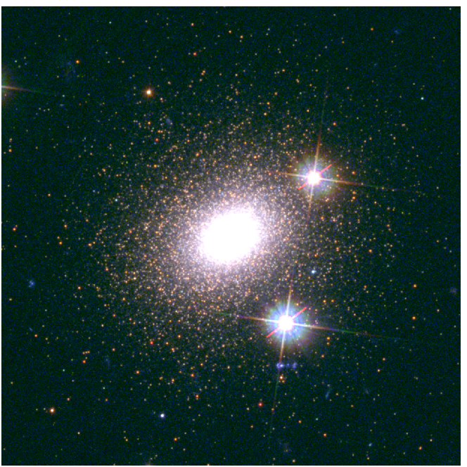
Figure 1: Stacked three-colour image (F336W$+$F438W$+$F606W) of a field 39.5$\times$39.5 arcsec² centred on G1. North is up, east is left.

Table 1: Description of the archival HST images reduced in this analysis.

MAYALL II (G1)
Program	Epoch	Filter	$N\times$ Exp. time	Instrument	PI
5464	1994.58	F555W	4 $\times$ 400 s	WFPC2	Rich
5464	1994.58	F814W	3 $\times$ 400 s	WFPC2	Rich
5907	1995.76	F555W	2 $\times$ 500 s $+$ 2 $\times$ 600 s	WFPC2	Jablonka
5907	1995.76	F814W	2 $\times$ 400 s $+$ 2 $\times$ 500 s	WFPC2	Jablonka
9767	2003.81	F555W	6 $\times$ 410 s	ACS/HRC	Gebhardt
12226	2011.01	F275W	2 $\times$1395 s $+$ 4 $\times$1465 s	WFC3/UVIS	Rich
12226	2010.85	F336W	6 $\times$ 889 s	WFC3/UVIS	Rich
12226	2011.01	F438W	2 $\times$1395 s $+$ 4 $\times$1465 s	WFC3/UVIS	Rich
12226	2010.85	F606W	6 $\times$ 889 s	WFC3/UVIS	Rich

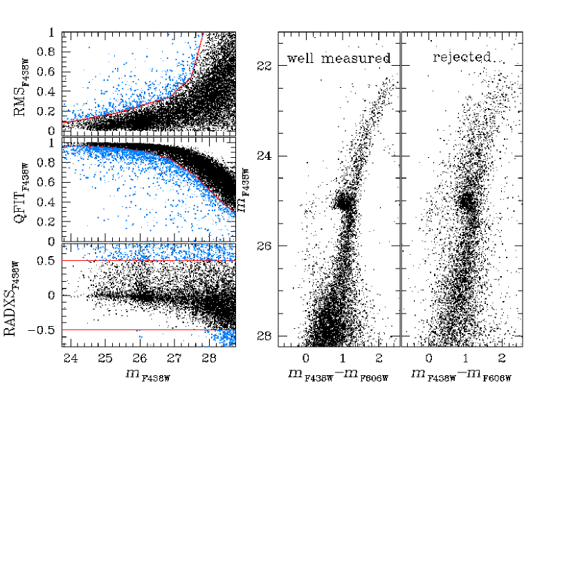
Figure 2: Selection of well-measured stars for G1. Left-hand panels show the selections (black points) for the filter F438W using the parameters RMS (top panel), QFIT (center panel), and RADXS (bottom panel). Middle and right panels show the $m_{\rm F606W}$ versus $m_{\rm F438W}-m_{F606W}$ CMD for the stars that pass the selection criteria and the rejected stars, respectively.

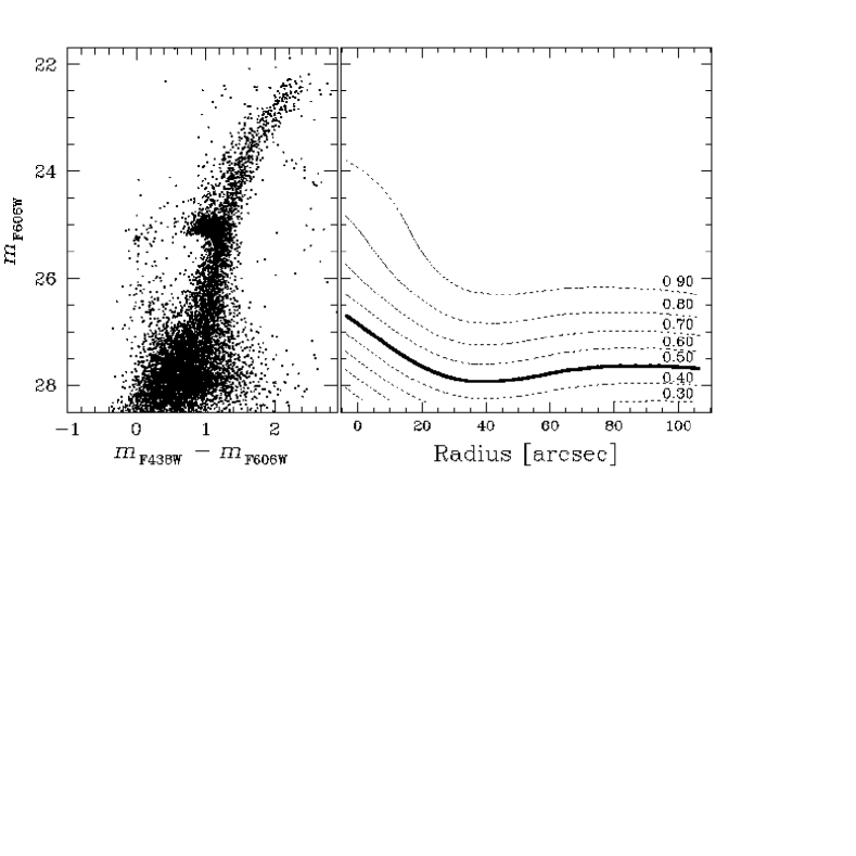
Figure 3: Left panel shows the $m_{\rm F606W}$ versus $m_{\rm F438W}-m_{\rm F606W}$ CMD of all the well measured stars in the field of view containing G1. Right panel shows the completeness levels of our catalogue as a function of the F606W magnitude and of the radial distance from the centre of the cluster.

Figure 4: Statistical removal of field stars. Top panels show the $m_{\rm F606W}$ versus $m_{\rm F438W}-m_{\rm F606W}$ CMDs of the cluster (left) and reference (right) fields. Bottom-left panel shows the $m_{\rm F606W}$ versus $m_{\rm F438W}-m_{\rm F606W}$ CMD of cluster-field stars after the decontamination; bottom-right panel shows the stars subtracted to the CMD of the cluster field.

In the majority of the analysed GCs, MPs have uniform metallicity and are characterised only by different helium content and light-element abundance. However, some massive clusters also show internal variations in heavy elements, including iron and s-process elements (e.g. Marino et al. 2015; Johnson et al. 2015). In particular, $\omega$ Cen, which is the most-massive Milky-Way GC ($\mathcal{M}=10^{6.4}\mathcal{M}_{\rm\odot}$, McLaughlin & van der Marel 2005), exhibits the most-extreme variation of iron, with [Fe/H] ranging from $\sim-2.2$ to $\sim-0.7$ (e.g. Norris et al. 1996; Johnson & Pilachowski 2010; Marino et al. 2011b).

Understanding the properties of MPs in GCs may constrain the models of formation of the GCs in the early Universe, the mechanisms responsible for the assembly of the halo, and the role of GCs in the re-ionization of the Universe (e.g., Renzini et al. 2015; Renzini 2017 and references therein).

Evidence of MPs in GCs belonging to external galaxies are widely reported in literature. Photometric detection of MPs in four GCs of the Fornax dSph have been reported by Larsen et al. (2014). Multiple sequences have also been observed in the CMDs of young and intermediate age clusters of the Small and Large Magellanic Clouds (see, e.g., Niederhofer et al. 2017a, b; Correnti et al. 2017; Milone et al. 2018a, 2017b and references therein), but the phenomenon that generates these multiple sequences may be different from that observed for old stellar systems. Spectroscopic detection of MPs in GCs of external galaxies have been reported, e.g., by Larsen et al. (2012, in the Fornax dSph ), Schiavon et al. (2013, in M 31), Mayya et al. (2013, in M81), Mucciarelli et al. (2009), Dalessandro et al. (2016), and Martocchia et al. (2018, in the Large and Small Magellanic Clouds).

In this context, the investigation of massive clusters in nearby galaxies is of great importance to understand whether the occurrence of MPs and the dependence on the mass of the host cluster are a peculiarity of Milky-Way GCs or are an universal phenomenon.

To address this issue, we investigate the presence of MPs in the GC Mayall II (G1, Sargent et al. 1977), in the nearby galaxy M 31, a cluster three times more massive than $\omega$ Cen ($\mathcal{M}=10^{7.2}\mathcal{M}_{\rm\odot}$, Meylan et al. 2001). G1 has been previously investigated by using Wide Field and Planetary Camera 2 photometry in the F555W and F814W bands (Rich et al. 1996; Meylan et al. 2001; Ma et al. 2007; Federici et al. 2012). Early evidence of metallicity variations is provided by Meylan et al. (2001) on the basis of the broadened RGB. It is noteworthy that G1 exhibits kinematic hints for a central intermediate mass black hole (Gebhardt et al. 2005).

In this work we present exquisite multi-band photometry of the stars hosted by G1, extracting their luminosities in six HST filters, from UV to optical bands (Section 2). We identify major features of the CMD of G1 never shown before and we analyse them to extract the main properties of the cluster stellar populations (Section 3). Finally, we compare the results obtained from G1 with those for massive Galactic GCs that present similar features in the CMD (Section 4), and we discuss them (Section 5) in the context of multiple stellar populations.

2 Observations and data reduction

For this work we reduced the archival HST data of G1 collected with the Wide Field and Planetary Camera 2 (WFPC2), with the High-Resolution Channnel (HRC) of the Advanced Camera for Surveys (ACS), and with the UVIS imager of the Wide Field Camera 3 (WFC3). WFPC2 data in F555W and F814W bands were collected within programs GO-5464 (PI: Rich) and GO-5907 (PI: Jablonka); observations in F555W with ACS/HRC were obtained within GO-9767 (PI: Gebhardt); WFC3/UVIS images in F275W, F336W, F438W, and F606W bands were taken for GO-12226 (PI: Rich). Table 1 gives the journal of observations used in this work. Figure 1 shows a stacked three-colour image of the G1 field.

To obtain high precision photometry, we perturbed library point spread functions (PSFs) to extract, for each image, a spatial- and time-varying array of PSFs, as already done in other works by our group (see, e.g., Bellini et al. 2017; Milone et al. 2018a; Nardiello et al. 2018a, b). These PSF arrays have been used to extract positions and fluxes of the stars on the images. We corrected the positions using the geometric distortion solutions given by Anderson & King (2003, WFPC2), Anderson & King (2004, ACS/HRC), Bellini & Bedin (2009) and Bellini et al. (2011, WFC3/UVIS). We used the Gaia DR2 catalogue (Gaia Collaboration et al. 2016; Gaia Collaboration et al. 2018) to transform the positions of the single catalogues in a common reference frame. We used the FORTRAN routine kitchen_sync2 (KS2, for details see Anderson et al. 2008; Bellini et al. 2017; Nardiello et al. 2018b) that takes as input the PSF arrays, the transformations and the images, and analyses all the images simultaneously to find the position and measure the flux of each source, after subtracting its neighbours. This routine allows us to obtain high precision photometry in crowded environments and of stars in the faint magnitude regime. We calibrated the output photometry into the Vega-mag system using, for WFPC2, the zero-points and the aperture corrections tabulated by Holtzman et al. (1995), for ACS/HRC the zero-points given by the “ACS Zeropoints Calculator” and the aperture corrections tabulated by Bohlin (2016), and for WFC3/UVIS the zero-points and the aperture corrections listed by Deustua et al. (2017).

To perform our analysis, we selected only well measured stars as in Nardiello et al. (2018a) on the basis of several diagnostic parameters output of the routine KS2 (see Nardiello et al. 2018b for details). The procedure is illustrated in Fig. 2 for the filter F438W, but it is the same for all the other filters. Briefly, we divided the distributions of the parameters RMS (the standard deviation of the mean magnitude divided $\sqrt{N-1}$ with $N$ the number of measurements) and QFIT (the quality-of-fit) in intervals of 0.5 magnitude and, in each magnitude bin, we calculated the 3.5$\sigma$-clipped average of the parameter and then the point 3.5$\sigma$ above the mean value of the parameter. We linearly interpolated these points (red line) and we excluded all the points above (in the case of the RMS) or below (for the QFIT) this line (azure points). Moreover, we excluded all the sources that have RADXS$>0.5$ (where RADXS is the shape parameter, defined in Bedin et al. 2008) and RADXS$<-0.5$ (bottom left-hand panel of Fig. 2), and for which the number of measurements is $N<2$. Middle-panel of Fig. 2 shows the $m_{\rm F606W}$ versus $m_{\rm F438W}-m_{F606W}$ CMD for the stars that pass the selections in F438W and F606W filters, while the right-hand panel shows the rejected stars.

2.1 Artificial stars and completeness

We estimated the completeness of our G1 catalogue using artificial stars (AS). We produced 100 000 ASs having magnitude $21.75\leq m_{\rm F606W}\leq 28.25$, flat luminosity function in F606W, colours that lie along the red giant branch (RGB) and the horizontal branch (HB) fiducial lines, and flat spatial distribution. For each AS in the input list, the routine KS2 added the star to each image, searched and measured it using the same approach used for real stars, and then removed the source and passed to the next AS (see Anderson et al. 2008 for details). Using this approach, if an artificial star is added on a crowded zone of the image (like the cluster center), comparing the input and output photometry of the artificial star we can estimate how much the crowding is affecting the measurement of a star located in that position.

To estimate the level of completeness, we considered an AS as recovered if the difference between the input and output positions is $<0.5$ pixel and the difference between the input and output $m_{\rm F606W}$ and $m_{\rm F438W}$ magnitudes is $<0.75$ mag.

Figure 3 illustrates the completeness of our catalogue: right panel shows the completeness contours in the $m_{\rm F606W}$ versus radial distance plane. Our catalogue has completeness $>50$% for stars with $m_{\rm F606W}\lesssim 26.5$ at all radial distances from the cluster centre.

2.2 Field decontamination

Due to the large distance of G1 and the short baselines of the observations, using proper motions to separate G1 members from field stars is not possible. We decontaminated the cluster CMD from background and foreground stars using the statistical approach (see, for example, Milone et al. 2018a). The procedure is illustrated in Fig. 4. We defined two circular regions: a cluster field containing G1 and a reference field nearby on the same CCD frame, covering the same area of the cluster field. The radius of each circular region is equal to 33.5 arcsec ($\sim 1.5\times r_{t}$, Ma et al. 2007). The stars of cluster and reference fields are showed in the $m_{\rm F606W}$ versus $m_{\rm F438W}-m_{\rm F606W}$ CMDs of top-left and top-right panels of Fig. 4, respectively. For each star $i$ in the reference field, we calculated the distance

where $C_{\rm F438W,F606W,cf}$ and $C^{i}_{\rm F438W,F606W,rf}$ are the $m_{\rm F438W}-m_{\rm F606W}$ colours of the stars in the cluster and reference fields, respectively. We flagged the closest star in the G1 field as a candidate to be subtracted. We associated to these flagged stars a random number $0\leq r_{i}\leq 1$ and we subtracted from the cluster field CMD the candidates with $r_{i}<c^{i}_{rf}/c^{i}_{cf}$, where $c^{i}_{rf}$ and $c^{i}_{cf}$ are the completeness of the star $i$ in the reference field and of the closest star in the cluster field. Bottom panels of Fig. 4 show the result of the decontamination: left panel show the $m_{\rm F606W}$ versus $m_{\rm F438W}-m_{\rm F606W}$ CMD of cluster field stars after the decontamination, while right panel shows the stars subtracted from the cluster field CMD. Note the similarity of G1 and field. Field is dominated by M31 stars whose CMD is similar to G1.

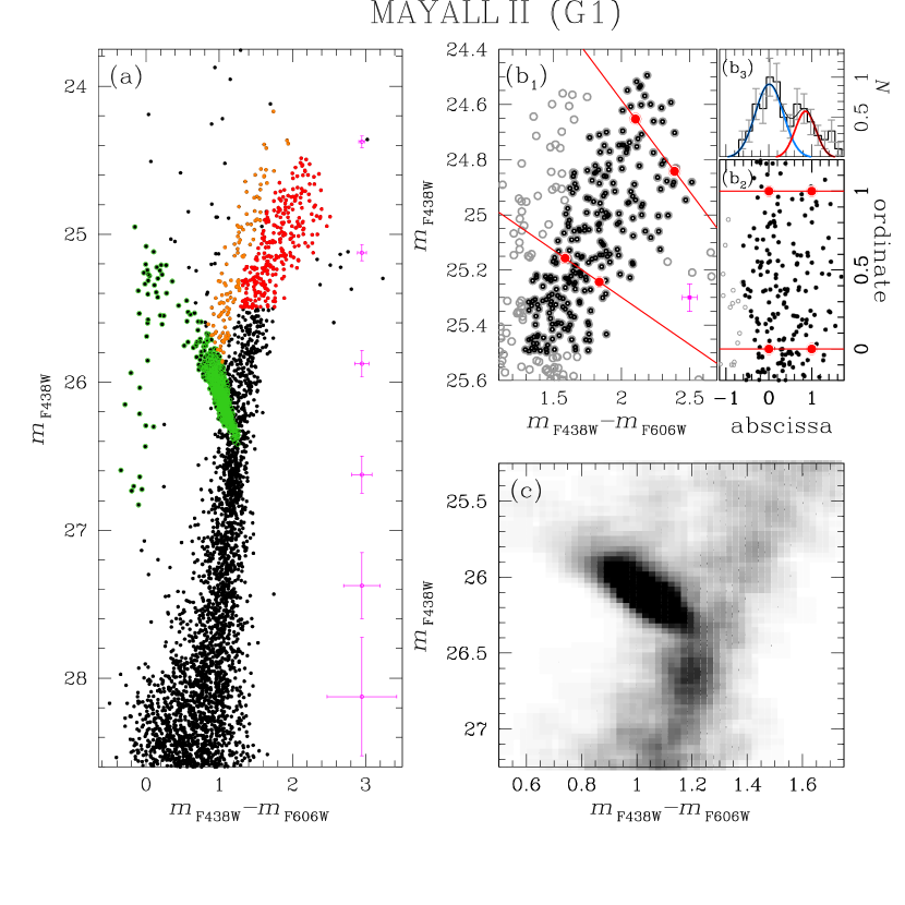
Figure 5: Overview of G1 features. Panel (a) shows the $m_{\rm F438W}$ versus $m_{\rm F438W}-m_{\rm F606W}$ CMD: RGB, HB, and AGB stars are highlighted in red, green, and orange, respectively. In magenta the observational errors in bins of 0.75 F438W magnitude. Panel (b₁) is a zoom-in around the upper RGB region, where the sequence is splitted in two; in magenta the median observational error. Panel (b₂) shows the verticalized RGB sequence; the ’abscissa’ distribution of the verticalized sequence is showed in panel (b₃). A bi-Gaussian function is fitted to the abscissa distribution. Panel (c) illustrates the Hess diagram around the CMD region containing the red clump and the RGB-bump.

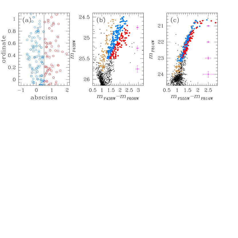
Figure 6: Panel (a) shows the verticalized RGB sequence: RGB a (red) and RGB b (blue) stars are divided by the line at ’abscissa’$=0.5$. Panels (b) and (c) show the RGB a (red) and RGB b (blue) stars in the $m_{\rm F438W}$ versus $m_{\rm F438W}-m_{\rm F606W}$ and $m_{\rm F814W}$ versus $m_{\rm F555W}-m_{\rm F814W}$ CMDs; AGB stars are plotted in orange.

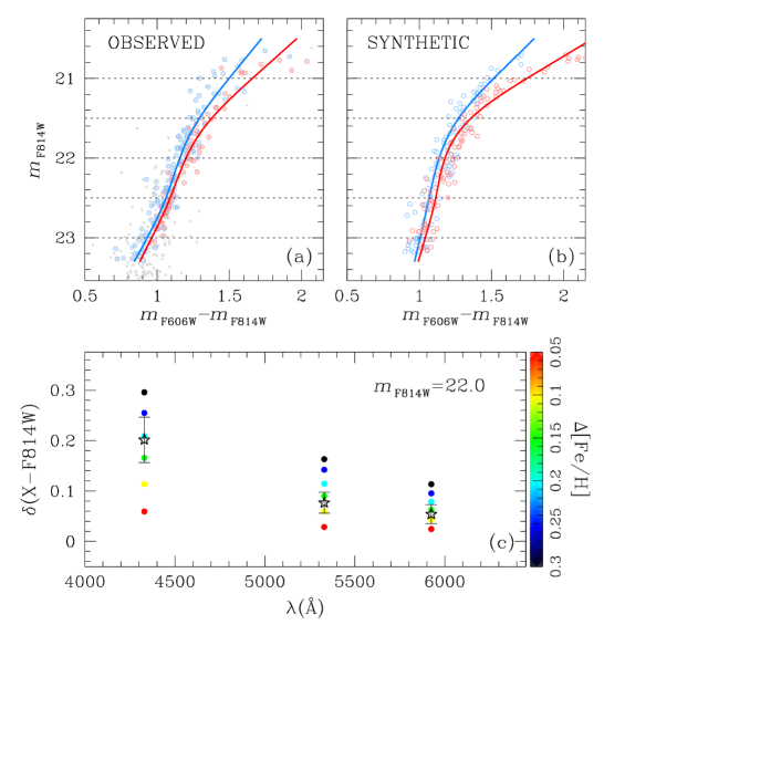
Figure 7: Procedure adopted to derive $\Delta$[Fe/H] between RGB a and RGB b. Panel (a) shows a zoom of the $m_{\rm F814W}$ versus $m_{\rm F606W}-m_{\rm F814W}$ CMD around the upper part of the RGB. In red and blue the fiducial lines for RGB a and RGB b, respectively. Panel (b) shows the synthetic CMD in the same filters, obtained using the models with [Fe/H]=$-0.85$ (blue fiducial line) and [Fe/H]=$-0.70$ (red fiducial line). Panel (c) shows the comparison between the colour difference $\delta({\rm X-F814W})^{\rm obs}$ (black stars) obtained from observed fiducial lines and the colour differences $\delta({\rm X-F814W})^{\rm synth}$ (points colour-coded as in the bar on the right) for different $\Delta$[Fe/H] at $m_{\rm F814W}^{\rm cut}=22.0$.

3 The CMD of G1

Left panel of Fig. 3 shows the $m_{\rm F606W}$ versus $m_{\rm F438W}-m_{\rm F606W}$ CMD of all the well measured stars in the field containing G1.

In panel (a) of Fig. 5 we plot the decontaminated $m_{\rm F438W}$ versus $m_{\rm F438W}-m_{\rm F606W}$ CMD for all the well measured sources of G1. We highlighted possible asymptotic giant branch (AGB), RGB, and HB stars in orange, red, and green, respectively. In the following we analyse the peculiarities of these sequences and we compare the main properties of the CMD of G1 with what observed in other massive Galactic GCs.

3.1 The upper part of the RGB

A visual inspection of the bright part of the $m_{\rm F438W}$ versus $m_{\rm F438W}-m_{\rm F606W}$ CMD (panel (a) of Fig. 5) reveals that the upper part of the RGB sequence is broadened in colour. The broadening becomes evident if we compare this sequence with the average observational errors in colour (magenta crosses ) in the same range of magnitudes. Also note that the fainter (and therefore affected by larger errors) blue HB is narrower than the brighter RGB, strengthening that the RGB broadening is intrinsic. This broadening was already observed by Meylan et al. (2001), and was associated to a spread in metallicity among RGB stars.

Panel (b₁) of Fig. 5 shows that the upper part of the RGB of G1 splits in two sequences. We verticalized the RGB using the same procedure adopted by Bellini et al. (2013, see also for details). As a result of the verticalization process, for each star we have a transformed colour and magnitude in a new plane ’ordinate’ versus ’abscissa’ (panel (b₂)). The distribution of the transformed colours of the RGB stars is shown in panel (b₃): the distribution is bimodal, with two clear peaks. We fitted the histogram with a bi-Gaussian function to derive the fraction of stars belonging to the two sequences. We found that the redder RGB (named RGB a) contains 32$\pm$2 % of the RGB stars, while the RGB b, that is on the blue side of the RGB, contains 68$\pm$2 % of the RGB stars.

In Fig. 6 we demonstrate that the bimodality of the upper part of the RGB is a real feature: panel (a) shows the verticalized RGB sequence as obtained in panels (b) of Fig. 5. We divided the verticalized sequence in two groups, on the basis of the gap in the RGB: the stars having ’abscissa’$<0.5$ (in blue, RGB b) and the stars with ’abscissa’$>0.5$ (in red, RGB a). To investigate if the separation of the two sequences is real, we used the approach adopted in Nardiello et al. (2015); Nardiello et al. (2018a): if the colour spread is due to photometric errors, a star of the RGB a sequence that is redder than the RGB b sequence in the $m_{\rm F438W}$ versus $m_{\rm F438W}-m_{F606W}$ CMD (panel (b) of Fig. 6), should have the same probability of being either red or blue in CMDs obtained with other combinations of filters. The fact that in the totally independent $m_{\rm F814W}$ versus $m_{\rm F555W}-m_{F814W}$ CMD (panel (c) of Fig. 6) RGB a and RGB b form two well-defined sequences demonstrates that the stars belonging to these two groups have indeed different properties.

3.2 Metallicity of G1 and spread of the RGB

In literature there are many estimates of the metallicity for G1, obtained using photometry (see, e.g., Stephens et al. 2001; Meylan et al. 2001; Bellazzini et al. 2003; Rich et al. 2005), integrated spectra (e.g., Huchra et al. 1991), and spectro-photometric Lick indices (Galleti et al. 2009). Huchra et al. (1991) obtained [Fe/H]=$-1.08\pm 0.09$ using integrated spectra; by the analysis of the CMDs, Meylan et al. (2001), Stephens et al. (2001), and Bellazzini et al. (2003) found [Fe/H]=$-0.95\pm 0.09$, [Fe/H]=$-1.22\pm 0.43$, and [Fe/H]=$-0.82\pm 0.26$ respectively; from spectro-photometric Lick indices Galleti et al. (2009) measured [Fe/H]=$-0.73\pm 0.15$; on average the metallicity of G1 stars is $\sim-0.95$.

As already discussed in the previous section, the RGB of G1 is strongly widened. Meylan et al. (2001) attributed this spread to variations of [Fe/H] among RGB stars of G1. In this section we investigate if this hypothesis is valid, comparing the observed split of the upper part of the RGB with theoretical models.

The procedure adopted is illustrated in Fig. 7. First, we derived for the observed RGB a and RGB b the fiducial lines. We derived the fiducial lines in the $m_{\rm F814W}$ versus $m_{\rm X}-m_{\rm F814W}$ CMDs, where X=F438W,F555W,F606W. The procedure to obtain a fiducial line is based on the naive estimator: we divided the RGB a (RGB b) sequence in intervals of $\delta=1$ F814W magnitudes. On these intervals we defined a grid of $N$ points separated by steps of width $\delta/10$ and we calculated the median colour and magnitude within the interval $m^{i}_{\rm F814W}<m_{\rm F814W}<m^{i}_{\rm F814W}+\delta$, with $i=1,...,N$; we interpolated these median points with a spline. An example of fiducial lines is shown in panel (a) of Fig. 7, where the red line is for RGB a and the blue line is for RGB b.

We obtained synthetic fiducial lines as follows: we considered a 12 Gyr $\alpha$-enhanced BaSTI isochrone (Pietrinferni et al. 2004, 2006, 2009) with a given [Fe/H], and we obtained a first guess synthetic CMD interpolating the isochrone on a vector of random $m_{\rm F814W}$ magnitudes, assuming a flat luminosity distribution. We broadened this synthetic CMD by adding to the colour of each synthetic star a random Gaussian noise, with a dispersion equal to the average colour error measured for upper RGB stars. Each synthetic CMD is composed by 10 000 synthetic stars. For each synthetic CMD we extracted synthetic fiducial lines using the same approach adopted for the observed CMD. Panel (b) of Fig. 7 shows the synthetic CMDs and the synthetic fiducial lines for two isochrones with [Fe/H]=$-0.85$ (blue) and [Fe/H]=$-0.70$ (red).

For each $m_{\rm F814W}$ versus $m_{\rm X}-m_{\rm F814W}$ observed CMD, we computed the colour difference $\delta({\rm X-F814W})^{\rm obs}$ between RGB a and RGB b fiducial lines, at 5 F814W magnitudes, $m_{\rm F814W}^{\rm cut}=$21.0, 21.5, 22.0, 22.5, 23.

We chose the model [Fe/H]=$-0.70$ as reference for RGB a and, for each $m_{\rm F814W}^{\rm cut}$, we computed the colour difference $\delta({\rm X-F814W})^{\rm synt}$ between the synthetic fiducial line for [Fe/H]=$-0.70$ and the fiducial lines for $-1.00<$[Fe/H]$<-0.75$, i.e., for $0.05<\Delta$[Fe/H]$<0.30$.

For each $m_{\rm F814W}^{\rm cut}$, we compare $\delta({\rm X-F814W})^{\rm obs}$ and $\delta({\rm X-F814W})^{\rm synt}$ to search for the best $\Delta$[Fe/H] that reproduce the observed colour difference in all the bands. Panel (c) of Fig. 7 shows, coloured from blue to red, the colour differences obtained from the models for $m_{\rm F814W}^{\rm cut}=22.0$; black stars are the observed points at the same magnitude level. In Table 2 we listed the $\Delta$[Fe/H] obtained for each $m_{\rm F814W}^{\rm cut}$. We computed the weighted average of all the $\Delta$[Fe/H], using as weight $1/\sigma_{\rm\Delta[Fe/H]}$, and we did so for three different cases: (i) the two populations have the same helium and C+N+O abundance (Scenario 1); (ii) the two populations share the same C+N+O content, but RGB a is populated by stars having primordial helium, while RGB b stars have $Y=0.30$ (Scenario 2); (iii) the two populations have the same helium content, but RGB b is populated by stars C+N+O-enhanced (Scenario 3). In the latter case, the C+N+O content is about a factor of two larger than the CNO sum of the mixture used for the standard $\alpha$-enhanced case (Pietrinferni et al. 2009). Because of the uncertainties on the bolometric corrections in blue and UV bands for the isochrones C+N+O-enhanced, for Scenario 3 we excluded the $\delta({\rm F438W-F814W})$ point in the computation of $\Delta$[Fe/H]. For the Scenario 1 we found that the split of the RGB is well reproduced with a mean metallicity difference of $\Delta$[Fe/H]$=0.15\pm 0.03$, while in case of Scenario 2 and 3 we found $\Delta$[Fe/H]$=0.12\pm 0.03$ and $\Delta$[Fe/H]$=0.14\pm 0.04$, respectively.

We want to highlight that a similar behaviour of the RGB could also be reproduced by a combination of variations of metallicity, helium, and C+N+O content (see discussion in Sect. 4.1).

Table 2: $\Delta$[Fe/H] values obtained for each $m_{\rm F814W}^{\rm cut}$

	$\Delta$[Fe/H]
$m^{\rm CUT}_{\rm F814W}$	Scenario 1	Scenario 2	Scenario 3
21.0	0.12 $\pm$ 0.04	0.10 $\pm$ 0.05	0.18 $\pm$ 0.05
21.5	0.18 $\pm$ 0.06	0.13 $\pm$ 0.06	0.18 $\pm$ 0.07
22.0	0.17 $\pm$ 0.05	0.12 $\pm$ 0.04	0.15 $\pm$ 0.05
22.5	0.16 $\pm$ 0.06	0.11 $\pm$ 0.05	0.11 $\pm$ 0.05
23.0	0.17 $\pm$ 0.06	0.12 $\pm$ 0.06	0.10 $\pm$ 0.05
average	0.15 $\pm$ 0.03	0.12 $\pm$ 0.03	0.14 $\pm$ 0.04

3.3 The HB of G1

We know that the metallicity is the parameter that mainly determine the morphology of the HB of a GC. However, some Galactic GCs, despite they have the same metallicity, present different HB morphologies. This is the so-called “2nd-parameter” problem. Many parameters have been suggested as candidates to explain the peculiarities observed for some Galactic GCs. Recently, Milone et al. (2014) have demonstrated that the extension of the HB correlates with the mass of the hosting GC. Milone et al. (2018b) show that the morphology of the HB is also correlated with the internal helium variations among the different populations hosted by GCs, demonstrating that HB morphology is strictly related to the presence of multiple populations (see also, e.g., D’Antona et al. 2002; Dalessandro et al. 2011, 2013). The HB morphology of M31 GCs and the effects of the second parameter have been analysed in many works in literature (see, e.g., Rich et al. 2005; Perina et al. 2012).

Already Rich et al. (1996) discovered that the HB of G1 is very populated on the red side, and that a few stars populate the blue side (see also Rich et al. 2013). In this paper we confirm that the HB of G1 is composed by a very populated red clump and we show for the first time the evidence of a very extended blue HB (green points in panel (a) of Fig. 5), more than expected and observed until now, even though it is an intermediate metallicity GC ([Fe/H]$\sim-0.95$).

Taking into account of the completeness of our sample, we found that the red clump and the blue side of HB of G1 contain $\sim 85$% and $\sim 15$% of HB stars, respectively. It has been demonstrated that Galactic GCs that show HB morphologies similar to that of G1 also host a small fraction of very high helium-enhanced stars (see, e.g., Caloi & D’Antona 2007; Busso et al. 2007; Bellini et al. 2013; Milone et al. 2014; Tailo et al. 2017) that populate the blue HB. We suggest that also G1 might host a small fraction ($\sim 15$ %) of highly helium-enhanced stars, that evolve into the blue side of the HB.

4 Comparison between G1 and Galactic GCs

In this section we compare the massive GC G1 in M31 with Galactic GCs of similar mass. We compared G1 with two Galactic GCs, NGC 6388, and NGC 6441, using the HUGS catalogues published by Nardiello et al. (2018b).

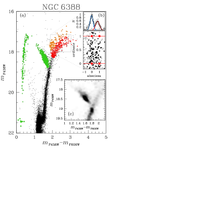
Figure 8: Overview of NGC 6388 features. Panel (a) shows the $m_{\rm F438W}$ versus $m_{\rm F438W}-m_{\rm F606W}$ CMD: HB, RGB and AGB stars are highlighted in green, red and orange, respectively. Panels (b) shows the verticalized RGB sequence using the stars of the grey box of panel (a); the ’abscissa’ distribution of the verticalized sequence is shown in the upper panel. A bi-Gaussian function is fitted to the abscissa distribution. Panel (c) illustrates the Hess diagram around the CMD region containing the red clump and the RGB bump.

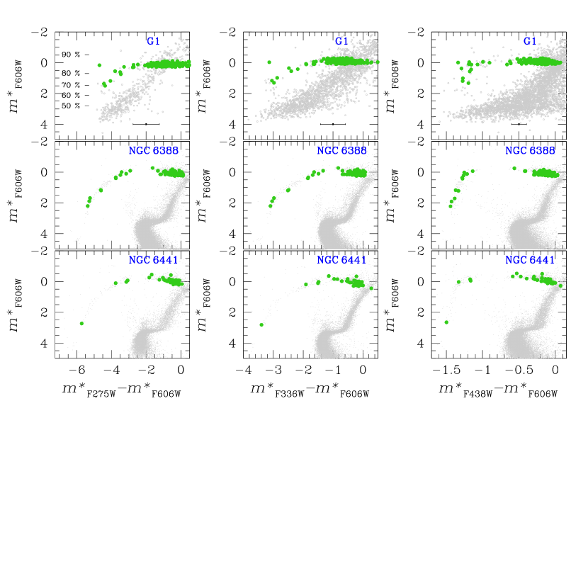
Figure 9: Transformed $m^{*}_{\rm F606W}$ versus $m^{*}_{\rm X}-m_{\rm F606W}$ CMDs, with X=F275W, F336W, and F438W, for the HB stars of G1 (first row), NGC 6388 (second row), NGC 6441 (third row). The left-hand panels are the $m^{*}_{\rm F606W}$ versus $m^{*}_{\rm F275W}-m_{\rm F606W}$ CMDs, the middle panels are the $m^{*}_{\rm F606W}$ versus $m^{*}_{\rm F336W}-m_{\rm F606W}$ CMDs, while the right-hand panels show the $m^{*}_{\rm F606W}$ versus $m^{*}_{\rm F438W}-m_{\rm F606W}$ CMDs of the GCs listed above. The green points are the HB stars located between $2.5\times r_{h}$ and $4.5\times r_{h}$ from the cluster centers. Top-left panel reports the completeness of G1 catalogue at different magnitude levels.

4.1 G1 versus NGC 6388

The GC NGC 6388 is a massive, metal-rich ([Fe/H]=$-0.45\pm 0.04$, Carretta et al. 2009) Galactic globular cluster, with an anomalously extended blue HB (for its metallicity).

From a visual inspection of the $m_{\rm F438W}$ versus $m_{\rm F438W}-m_{\rm F606W}$ CMD of G1 (panel (a) of Fig. 5) and NGC 6388 (panel (a) of Fig. 8) we note many common features including the well populated red clump, the extended blue HB, and the splitted RGB.

As already demonstrated by Bellini et al. (2013), the upper part of the RGB of NGC 6388 splits in two sequences in the $m_{\rm F438W}$ versus $m_{\rm F438W}-m_{\rm F606W}$ CMD. Panels (b) of Fig. 8 shows the verticalized RGB sequence (bottom) and the histogram of the “abscissa” distribution (top) for NGC 6388, obtained as in Sect. 3. By least-squares fitting a bi-Gaussian function, we found that the RGB on the red side contains $42\pm 2$ % of RGB stars, while the remaining $58\pm 3$ % stars are on the blue side. This result is very similar to what we found for G1.

In Sect. 3.2 we have tested the hypothesis that the RGB split observed for G1 is due to a metallicity variation of $\sim 0.15$ dex between the two populations. For NGC 6388, Carretta et al. (2007) found no intrinsic metallicity spread from spectroscopic measurements of RGB stars. A possible explanation of the RGB split could be a variation of the C+N+O content between the two populations, that implies also an SGB split in the optical CMDs. The SGB split for NGC 6388 was noticed by Bellini et al. (2013). Unfortunately, on the dataset used in this work, we are not able to distinguish between metallicity or C+N+O variations as cause of the RGB split observed for G1, because the SGB stars of G1 are too faint to be measured.

The HB morphologies of G1 and NGC 6388 are also very similar (in green in Figs. 5 and 8). Both HBs present a populated red clump, containing $\sim 85$-$90$ % of HB stars and well spread in magnitude. Tailo et al. (2017) showed that the red side of the HB of NGC 6388 is compatible with the presence of He-enriched stars ($\Delta Y\sim 0.08$).

The extended blue HB of G1 is very similar to that of NGC 6388. In the case of NGC 6388, Busso et al. (2007) and Tailo et al. (2017) showed that stars on the blue side of the HB of NGC 6388 are very helium-enriched, up to $\Delta Y\sim 0.13$ for the bluest ones.

There are few differences between the two clusters that must be taken into account in this analysis. First of all, NGC 6388 is more metal-rich ([Fe/H]=$-0.45\pm 0.04$, Carretta et al. 2009) than G1 ([Fe/H]$\sim-0.95$). Moreover, the present-day mass of NGC 6388 ($\sim 2\times 10^{6}\,M_{\odot}$, Boyles et al. 2011), is almost one order of magnitude smaller than G1 mass ($\sim 1.5\times 10^{7}\,M_{\odot}$ Meylan et al. 2001). Finally, the position of the two clusters in the host galaxy is totally different: NGC 6388 is a bulge Galactic GC, while G1 is projected at 40 kpc in the halo of M31.

4.2 Multi-band comparison of the HB morphologies

The dataset used in this work allows us to analyse the extended HB of G1 from the near UV to the visible.

To compare the HB morphology of G1 with that of other Galactic GCs, for each $m_{\rm F606W}$ versus $c_{\rm X}=m_{\rm X}-m_{\rm F606W}$ CMD, where X=F275W, F336W, and F438W, we performed a translation of the entire CMD as follows: we calculated the 96th percentile (on the red side) of the HB colour distribution, $c_{\rm 96th,X}$, and the associated magnitude, $m_{\rm 96th,F606W}$ Then, we defined a new colour $c^{*}_{\rm X}=c_{\rm X}-c_{\rm 96th,X}$ and magnitude $m^{*}_{\rm F606W}=m_{\rm F606W}-m_{\rm 96th,F606W}$.

To compare the HBs of G1 and of the Galactic GCs NGC 6388 and NGC 6441, avoiding the very low completeness of the G1 catalogue in the center region, we selected only the HB stars between $2.5\times r_{h}$ and $4.5\times r_{h}$ from the cluster centers, where $r_{h}$ is the half-light radius ($r_{h}=$1.7, 31.2, and 34.2 arcsec for G1, NGC 6388, and NGC 6441, respectively, Harris 1996; Ma et al. 2007).

The first row of Fig. 9 shows the multiband photometry of the HB of G1 (green points). In the left panel we also report the completeness level. We compared the HB morphology of G1 with that of two Galactic GCs that are massive ($\gtrsim 10^{6}\,M_{\odot}$), that host stars highly enriched in helium ($Y\sim 0.30-0.35$) and that have a populated red clump: NGC 6388 (2nd row of Fig. 9) and NGC 6441 (3rd row of Fig. 9). We highlighted in green their HB stars.

The GCs NGC 6388 and NGC 6441 are [Fe/H]-rich clusters ($\sim-0.45$; Carretta et al. 2009) located in the bulge of the Milky Way. Both clusters show a peculiar HB morphology: a very populated red clump (85-90% of HB stars) and an extended blue HB (Rich et al. 1997). Even if these two clusters seem to be twins, the chromosome maps of RGB stars (Milone et al. 2017a) are very different.

A comparison between the first, the second and the third row of Fig. 9 illustrates how the HB morphology of G1 is similar to that of the two selected Galactic GCs in all the analysed filters: the populated and extended red clumps, and the blue HB that covers about the same colour ranges are common features to these three GCs.

We know that both the red clumps of NGC 6388 and of NGC 6441 host stars with primordial helium content and helium enhancement by $\Delta Y\sim 0.08-0.1$, while the blue HB is populated by stars that have helium content $Y>0.35$ (Tailo et al. 2017). It is possible that a similar helium enhancement might plausibly explain the extended HB of G1.

The GCs NGC 6388 and NGC 6441 host stars that form an extreme HB (eHB, Bellini et al. 2013; Brown et al. 2016, see also Fig. 8). These stars are located mainly in the center of the clusters. The cluster G1 does not show eHB stars: we attribute the lack of such stars to the extreme crowding and consequent low completeness at these magnitudes in the central regions of the cluster.

5 Summary

In this work we presented a multi-band analysis of the CMDs of the GC Mayall II (G1) located in the halo of M31. We used HST data collected with filters that cover wavelengths from $\sim 250$ nm to $\sim 950$ nm. This is the first time that G1 is observed in UV and blue filters.

The high accuracy photometry extracted from HST data with new, advanced tools, has allowed us to extract for the first time a deep CMD (magnitude limits $V\sim 28.5$, $\sim 3$ magnitudes below the HB level) for this cluster. The $m_{\rm F606W}$ versus $m_{\rm F438W}-m_{\rm F606W}$ CMD shows new features never observed until now: a wide, likely bifurcated RGB, an extended blue HB, and populated RGB bump, AGB and red clump.

We show that the upper part of the RGB of G1 splits in two real sequences in the $m_{\rm F438W}$ versus $m_{\rm F438W}-m_{\rm F606W}$ CMD, as for the Galactic GC NGC 6388. We derive the fraction of stars within each sequence and we found the the redder sequence (RGB a) includes $\sim 32$ % of RGB stars, while the bluer RGB b sequence contains the remaining $\sim 68$ %.

We tested the hypothesis of [Fe/H]-variations to explain the RGB split, comparing the observed fiducial lines of the two populations with synthetic fiducial lines obtained using models. We found that the RGB split could be reproduced assuming that the two populations have a difference in [Fe/H] of $\Delta$[Fe/H]$=0.15\pm 0.03$ if the populations share the same helium and C+N+O content, $\Delta$[Fe/H]$=0.12\pm 0.03$ if the two populations have different helium content and the same C+N+O content, and $\Delta$[Fe/H]$=0.14\pm 0.04$ if the two populations share the same helium abundance but have different C+N+O content.

We compared the HB morphology of G1 with that of massive Galactic GCs that present a populated red clump. We found many similarities with the HBs of NGC 6388 and NGC 6441: a populated red clump ($>85$ % of HB stars) and an extended blue HB, despite these GCs are [Fe/H]-rich. We know that the red clump and the blue HB of NGC 6388 and NGC 6441 are populated by stars helium enriched by $\Delta Y\sim 0.08$ and $\Delta Y\sim 0.13$, respectively. Given the similarity between the HB morphologies of G1 and NGC 6388/NGC 6441, we can conclude that also HB stars of G1 may be helium enriched. An additional proof is given by the correlation found by Milone et al. (2018b) for Galactic GCs between the maximum internal helium variation and the mass of the cluster: more massive clusters have larger internal maximum helium variation. Because G1 is $\sim 3$ times more massive than $\omega$ Cen, the most massive GC in the Milky Way ($\sim 4\times 10^{6}M_{\odot}$, D’Souza & Rix 2013), we expected that the maximum internal helium variation among G1 stars is high, with $\Delta Y\gtrsim 0.1$.

All the results obtained in this work represent a proof that G1 hosts multiple stellar populations, characterised by different chemical properties. Moreover, some evidence tell us that G1 could belong to the group of “anomalous” GCs, that host populations with different C+N+O contents and/or [Fe/H]-content (as already suggested by Meylan et al. 2001). In the Milky Way a significant fraction of globular clusters belongs to the group of “anomalous” GCs ($\omega$ Cen, M22, NGC 5286, M54, M19, M2, NGC 6934, etc., see, e.g., Norris et al. 1996; Carretta et al. 2010; Marino et al. 2011a; Yong et al. 2014; Marino et al. 2015; Johnson et al. 2015; Johnson et al. 2017; Marino et al. 2018), and the discovery of a GC in M31 with similar characteristics means that these kind of clusters are not a prerogative of our Galaxy. Unfortunately, the dataset used in this work is not sufficient to constraint the chemical properties of this GC and of its populations, and more multi-band photometric observations are required to trace the formation and evolution of G1.

References

- Anderson & King (2003) Anderson J., King I. R., 2003, PASP, 115, 113
- Anderson & King (2004) Anderson J., King I. R., 2004, Technical report, Multi-filter PSFs and Distortion Corrections for the HRC
- Anderson et al. (2008) Anderson J., et al., 2008, AJ, 135, 2055
- Bedin et al. (2008) Bedin L. R., King I. R., Anderson J., Piotto G., Salaris M., Cassisi S., Serenelli A., 2008, ApJ, 678, 1279
- Bellazzini et al. (2003) Bellazzini M., Cacciari C., Federici L., Fusi Pecci F., Rich M., 2003, A&A, 405, 867
- Bellini & Bedin (2009) Bellini A., Bedin L. R., 2009, PASP, 121, 1419
- Bellini et al. (2011) Bellini A., Anderson J., Bedin L. R., 2011, PASP, 123, 622
- Bellini et al. (2013) Bellini A., et al., 2013, ApJ, 765, 32
- Bellini et al. (2017) Bellini A., Anderson J., Bedin L. R., King I. R., van der Marel R. P., Piotto G., Cool A., 2017, ApJ, 842, 6
- Bohlin (2016) Bohlin R. C., 2016, AJ, 152, 60
- Boyles et al. (2011) Boyles J., Lorimer D. R., Turk P. J., Mnatsakanov R., Lynch R. S., Ransom S. M., Freire P. C., Belczynski K., 2011, ApJ, 742, 51
- Brown et al. (2016) Brown T. M., et al., 2016, ApJ, 822, 44
- Busso et al. (2007) Busso G., et al., 2007, A&A, 474, 105
- Caloi & D’Antona (2007) Caloi V., D’Antona F., 2007, A&A, 463, 949
- Carretta et al. (2007) Carretta E., et al., 2007, A&A, 464, 967
- Carretta et al. (2009) Carretta E., Bragaglia A., Gratton R., D’Orazi V., Lucatello S., 2009, A&A, 508, 695
- Carretta et al. (2010) Carretta E., et al., 2010, A&A, 520, A95
- Correnti et al. (2017) Correnti M., Goudfrooij P., Bellini A., Kalirai J. S., Puzia T. H., 2017, MNRAS, 467, 3628
- D’Antona et al. (2002) D’Antona F., Caloi V., Montalbán J., Ventura P., Gratton R., 2002, A&A, 395, 69
- D’Souza & Rix (2013) D’Souza R., Rix H.-W., 2013, MNRAS, 429, 1887
- Dalessandro et al. (2011) Dalessandro E., Salaris M., Ferraro F. R., Cassisi S., Lanzoni B., Rood R. T., Fusi Pecci F., Sabbi E., 2011, MNRAS, 410, 694
- Dalessandro et al. (2013) Dalessandro E., Salaris M., Ferraro F. R., Mucciarelli A., Cassisi S., 2013, MNRAS, 430, 459
- Dalessandro et al. (2016) Dalessandro E., Lapenna E., Mucciarelli A., Origlia L., Ferraro F. R., Lanzoni B., 2016, ApJ, 829, 77
- Deustua et al. (2017) Deustua S. E., Mack J., Bajaj V., Khandrika H., 2017, Technical report, WFC3/UVIS Updated 2017 Chip-Dependent Inverse Sensitivity Values
- Federici et al. (2012) Federici L., Cacciari C., Bellazzini M., Fusi Pecci F., Galleti S., Perina S., 2012, A&A, 544, A155
- Gaia Collaboration et al. (2016) Gaia Collaboration et al., 2016, A&A, 595, A2
- Gaia Collaboration et al. (2018) Gaia Collaboration Brown A. G. A., Vallenari A., Prusti T., de Bruijne J. H. J., Babusiaux C., Bailer-Jones C. A. L., 2018, preprint, (arXiv:1804.09365)
- Galleti et al. (2009) Galleti S., Bellazzini M., Buzzoni A., Federici L., Fusi Pecci F., 2009, A&A, 508, 1285
- Gebhardt et al. (2005) Gebhardt K., Rich R. M., Ho L. C., 2005, ApJ, 634, 1093
- Harris (1996) Harris W. E., 1996, AJ, 112, 1487
- Holtzman et al. (1995) Holtzman J. A., Burrows C. J., Casertano S., Hester J. J., Trauger J. T., Watson A. M., Worthey G., 1995, PASP, 107, 1065
- Huchra et al. (1991) Huchra J. P., Brodie J. P., Kent S. M., 1991, ApJ, 370, 495
- Johnson & Pilachowski (2010) Johnson C. I., Pilachowski C. A., 2010, ApJ, 722, 1373
- Johnson et al. (2015) Johnson C. I., Rich R. M., Pilachowski C. A., Caldwell N., Mateo M., Bailey III J. I., Crane J. D., 2015, AJ, 150, 63
- Johnson et al. (2017) Johnson C. I., Caldwell N., Rich R. M., Mateo M., Bailey III J. I., Clarkson W. I., Olszewski E. W., Walker M. G., 2017, ApJ, 836, 168
- Larsen et al. (2012) Larsen S. S., Brodie J. P., Strader J., 2012, A&A, 546, A53
- Larsen et al. (2014) Larsen S. S., Brodie J. P., Grundahl F., Strader J., 2014, ApJ, 797, 15
- Ma et al. (2007) Ma J., et al., 2007, MNRAS, 376, 1621
- Marino et al. (2011a) Marino A. F., et al., 2011a, A&A, 532, A8
- Marino et al. (2011b) Marino A. F., et al., 2011b, ApJ, 731, 64
- Marino et al. (2015) Marino A. F., et al., 2015, MNRAS, 450, 815
- Marino et al. (2018) Marino A. F., et al., 2018, ApJ, 859, 81
- Martocchia et al. (2018) Martocchia S., et al., 2018, MNRAS, 477, 4696
- Mayya et al. (2013) Mayya Y. D., Rosa-González D., Santiago-Cortés M., Rodríguez-Merino L. H., Vega O., Torres-Papaqui J. P., Bressan A., Carrasco L., 2013, MNRAS, 436, 2763
- McLaughlin & van der Marel (2005) McLaughlin D. E., van der Marel R. P., 2005, ApJS, 161, 304
- Meylan et al. (2001) Meylan G., Sarajedini A., Jablonka P., Djorgovski S. G., Bridges T., Rich R. M., 2001, AJ, 122, 830
- Milone et al. (2009) Milone A. P., Stetson P. B., Piotto G., Bedin L. R., Anderson J., Cassisi S., Salaris M., 2009, A&A, 503, 755
- Milone et al. (2014) Milone A. P., et al., 2014, ApJ, 785, 21
- Milone et al. (2017a) Milone A. P., et al., 2017a, MNRAS, 464, 3636
- Milone et al. (2017b) Milone A. P., et al., 2017b, MNRAS, 465, 4363
- Milone et al. (2018a) Milone A. P., et al., 2018a, MNRAS, 477, 2640
- Milone et al. (2018b) Milone A. P., et al., 2018b, MNRAS, 481, 5098
- Mucciarelli et al. (2009) Mucciarelli A., Origlia L., Ferraro F. R., Pancino E., 2009, ApJ, 695, L134
- Nardiello et al. (2015) Nardiello D., Milone A. P., Piotto G., Marino A. F., Bellini A., Cassisi S., 2015, A&A, 573, A70
- Nardiello et al. (2018a) Nardiello D., et al., 2018a, MNRAS, 477, 2004
- Nardiello et al. (2018b) Nardiello D., et al., 2018b, MNRAS, 481, 3382
- Niederhofer et al. (2017a) Niederhofer F., et al., 2017a, MNRAS, 464, 94
- Niederhofer et al. (2017b) Niederhofer F., et al., 2017b, MNRAS, 465, 4159
- Norris et al. (1996) Norris J. E., Da Costa G. S., Freeman K. C., Mighell K. J., 1996, in Morrison H. L., Sarajedini A., eds, Astronomical Society of the Pacific Conference Series Vol. 92, Formation of the Galactic Halo…Inside and Out. p. 375
- Perina et al. (2012) Perina S., Bellazzini M., Buzzoni A., Cacciari C., Federici L., Fusi Pecci F., Galleti S., 2012, A&A, 546, A31
- Pietrinferni et al. (2004) Pietrinferni A., Cassisi S., Salaris M., Castelli F., 2004, ApJ, 612, 168
- Pietrinferni et al. (2006) Pietrinferni A., Cassisi S., Salaris M., Castelli F., 2006, ApJ, 642, 797
- Pietrinferni et al. (2009) Pietrinferni A., Cassisi S., Salaris M., Percival S., Ferguson J. W., 2009, ApJ, 697, 275
- Piotto et al. (2015) Piotto G., et al., 2015, AJ, 149, 91
- Renzini (2017) Renzini A., 2017, MNRAS, 469, L63
- Renzini et al. (2015) Renzini A., et al., 2015, MNRAS, 454, 4197
- Rich et al. (1996) Rich R. M., Mighell K. J., Freedman W. L., Neill J. D., 1996, AJ, 111, 768
- Rich et al. (1997) Rich R. M., et al., 1997, ApJ, 484, L25
- Rich et al. (2005) Rich R. M., Corsi C. E., Cacciari C., Federici L., Fusi Pecci F., Djorgovski S. G., Freedman W. L., 2005, AJ, 129, 2670
- Rich et al. (2013) Rich R. M., Piotto G., Reitzel D., Origlia L., Bedin L., 2013, in American Astronomical Society Meeting Abstracts #221. p. 213.04
- Sargent et al. (1977) Sargent W. L. W., Kowal C. T., Hartwick F. D. A., van den Bergh S., 1977, AJ, 82, 947
- Schiavon et al. (2013) Schiavon R. P., Caldwell N., Conroy C., Graves G. J., Strader J., MacArthur L. A., Courteau S., Harding P., 2013, ApJ, 776, L7
- Stephens et al. (2001) Stephens A. W., et al., 2001, AJ, 121, 2597
- Tailo et al. (2017) Tailo M., et al., 2017, MNRAS, 465, 1046
- Yong et al. (2014) Yong D., et al., 2014, MNRAS, 441, 3396