Experimental verification of the inertial theorem control protocols

Abstract

An experiment based on a trapped Ytterbium ion validates the inertial theorem for the $SU(2)$ algebra. The qubit is encoded within the hyperfine states of the atom and controlled by RF fields. The inertial theorem generates an analytical solution for non-adiabatically driven systems that are ‘accelerated’ slowly, bridging the gap between the sudden and adiabatic limits. These solutions are shown to be stable to small deviations, both experimentally and theoretically. As a result, the inertial solutions pave the way to rapid quantum control of closed, as well as open quantum systems. For large deviations from the inertial condition, the amplitude diverges while the phase remains accurate.

1 Introduction

Progress in contemporary quantum technology requires precise control of quantum dynamics [1, 2, 3, 4, 5, 6, 7, 8, 9, 10, 11, 12, 13, 14, 15, 16, 17, 18, 19, 20]. To answer the demand, a ”universal” vocabulary of control techniques has emerged. They have been applied across a broad range of experimental platforms, such as NV-centers [21, 22, 23], trapped ions [2, 24, 25], and Josephson devices [26, 27, 28]. These techniques are encapsulated within the theoretical framework of quantum control theory [29, 30, 1, 31].

This theory formulates the control problem by addressing three main topics:

1. Controllability, i.e., the conditions on the dynamics that allow obtaining the objective.

2. Constructive mechanisms of control, the problem of synthesis.

3. Optimal control strategies and quantum speed limits.

The first issue controlability of unitary dynamics of closed quantum system has been formulated employing Lie algebra techniques [30, 32, 33]. In this case, the Hamiltonian of the system is separated into drift and control terms

$$\hat{H}\left({t}\right)=\hat{H}_{0}+\sum_{j}g_{j}\left({t}\right)\hat{G}_{j}~{}~{},$$ (1)

where $\hat{H}_{0}$ is the free system Hamiltonian, $g_{j}(t)$ are the control fields and $\hat{G}_{j}$ are control operators. The system is unitary controllable provided that the Lie algebra, spanned by the nested commutators of $\hat{H}_{0}$ and $\hat{G}_{j}$, is full rank [30, 32, 33, 34].

When addressing the quantum control challenge, it is reassuring that a solution exists, nevertheless, the practical problem of finding a control protocol has not been solved. For this task a pragmatic approach has been developed, formulating the control problem as an optimization problem, leading to optimal control theory [35, 36, 37, 1]. This approach has achieved significant success in solving specific control problems. However, the drawback is that obtaining the control protocol relies on a specific numerical scheme which might be difficult to obtain and to generalize [38].

The present study is devoted to the experimental study of constructive mechanisms of control. Experimental realization based on quantum control impose additional requirements: (i)The control protocol should be robust under experimental errors and (ii) the mechanism should be clear and simple to generalize. These considerations have singled out the adiabatic protocols which have dominated the control field, across all platforms [39, 40]. Adiabatic methods are based on the adiabatic theorem which loosely states that the system will follow an eigenvalue of the instantaneous Hamiltonian, provided that the change in time is slow relative to the time associated with the relevant energy gaps [41, 42]. The fact that the Hamiltonian is an invariant of the dynamics enables a simple implementation of the control protocol by choosing the initial and final states as eigenstates of the Hamiltonian. The adiabatic condition on the change in the Hamiltonian will then generate the desired transition. The robustness of such a protocol stems from the redundancy in the intermediate Hamiltonian, which allow variations in the protocol, provided the changes are sufficiently slow. This implies that the adiabatic protocol timescale is large relative to the system free dynamics. The relatively long protocol durations mean that the adiabatic protocols become prone to environmental noise. This fact is one of the major disadvantages of the adiabatic method.

The present study is devoted to an experimental exploration for rapid alternative control protocol, which are based on the inertial theorem [43]. Such protocols are termed inertial protocols and are based on time-dependent invariants of the dynamics, beyond the adiabatic approximation. They serves as natural replacements of the instantaneous Hamiltonian of the adiabatic protocols. The inertial theorem follow a similar procedure as the standard adiabatic theorem [44]. As a consequence, the inertial and adiabatic solutions share a similar structure, which implies that the positive features of robustness and simplicity are maintained without paying the price of long timescales. The experimental demonstration of the theory is based on the $SU(2)$ algebra, which is realized by ¹⁷¹Yb⁺ ion confined in a Paul trap [45]

2 Inertial theory and solution

For a quantum control scheme to be generic, it has to rely on simple principles that apply across many platforms. The control procedure requires the formulation of a dynamical map $\Lambda_{t}$ from an initial state $\hat{\rho}\left({0}\right)$, to the final state $\hat{\rho}(t)=\Lambda_{t}\hat{\rho}(0)=\hat{U}\hat{\rho}(0)\hat{U}^{\dagger}$. The dynamical map is generated by the control Hamiltonian Eq. (1):

$$i\frac{\partial}{\partial t}\hat{U}(t)=\hat{H}(t)\hat{U}(t)~{}~{}~{}~{}\textrm{with}~{}~{}~{}~{}\hat{U}(0)=\hat{I}~{}~{},$$ (2)

where the convention $\hbar=1$ is used throughout this paper.

The major obstacle in generating such a map from a time-dependent control Hamiltonian is the time-ordering operation, resulting from the fact that $[\hat{H}(t),\hat{H}(t^{\prime})]\neq 0$. The adiabatic control circumvents this problem by employing a slow drive $g_{j}(t)$, allowing an approximate description in terms of the instantaneous eigenstates [46, 42, 47, 48, 49]. At the other extreme, the sudden limit, the control is so fast that it overshadows the dynamics generated by the drift Hamiltonian $\hat{H}_{0}$. This leads to an instantaneous change of the Hamiltonian, while leaving the system’s state unaffected.

The inertial dynamics and control paradigm serves as a compromise between the two extremes. It is based on the inertial theorem [43], which introduces an explicit solution of the dynamical map $\Lambda_{t}$ under certain restrictions. The theorem is formulated in Liouville space, a vector space of system operators $\{\hat{X}\}$, endowed with an inner product $\left({\hat{X_{i}},\hat{X_{j}}}\right)\equiv\textrm{tr}\left({\hat{X_{i}}^{\dagger}\hat{X_{j}}}\right)$ [50, 51, 52]. In Liouville space, the system’s dynamics are represented in terms of a basis of orthogonal operators $\{\hat{B}\}$, spanning the space. For example, the currently studied $SU(2)$ algebra can be completely characterized by a time-independent operator basis constructed from the Pauli operators $\{\hat{I},\hat{\sigma}_{x},\hat{\sigma}_{y},\hat{\sigma}_{z}\}$. The chosen (ordered) operator basis then defines a state in Liouville space. Note, that a time-dependent operator basis can also be chosen, $\{\vec{v}\left({t}\right)\}\equiv\{\hat{v}_{1}\left({t}\right),\dots,\hat{v}_{N}\left({t}\right)\}^{T}$, where $N$ the Liouville space dimension. This possibility serves as a major component in the inertial theorem and construction of inertial solutions.

The dynamics in Liouville space can be solved by substituting the chosen basis $\vec{v}\left({t}\right)$ into the Heisenberg equation of motion,

$$\frac{d}{dt}\vec{v}^{H}\left({t}\right)=\hat{U}^{\dagger}\left({t,0}\right)\left[{\left({i\left[{\hat{H}\left({t}\right),\bullet}\right]+\frac{\partial}{\partial t}}\right)\vec{v}\left({t}\right)}\right]\hat{U}^{\dagger}\left({t,0}\right)~{}~{},$$ (3)

where superscript $H$ signifies that the operators are in the Heisenberg picture.

We next consider a finite time-dependent basis, forming a closed Lie algebra, this guarantees that Eq. (3) can be solved within the basis [53]. For a closed Lie algebra, equation (3) has the simple form

$$\frac{d}{dt}\vec{v}^{H}\left({t}\right)={-i{\cal{M}}\left({t}\right)}\vec{v}^{H}\left({t}\right)~{}~{},$$ (4)

where ${\cal{M}}\left({t}\right)$ is a finite matrix with time-dependent elements and $\vec{v}\left({t}\right)$ is a vector .

The inertial solutions are obtained by searching for a driving protocol that allows solving Eq. (4) explicitly. These then enable extending the exact solutions for a broad range of protocols employing the inertial approximation. By choosing a unique driving protocol and the suitable time-dependent operator basis, the dynamical equation can be expressed as

$${\cal{M}}\left({t}\right)={\cal P}\left({\vec{\chi}}\right){\cal D}\left({\vec{\chi},\vec{\Omega}}\right){\cal P}^{-1}\left({\vec{\chi}}\right)~{}~{}.$$ (5)

Here, ${\cal{P}}\left({\vec{\chi}}\right)$ is an invertible matrix, which depends on the inertial coefficients $\{\chi_{k}\}$ (for conciseness they are expressed in terms of the vector $\vec{\chi}=\{\chi_{1},\dots,\chi_{K}\}$), and ${\cal{D}}=\textrm{diag}\left({\lambda_{1}\left({\vec{\chi}}\right)\Omega_{1}\left({t}\right),...,\lambda_{N}\left({\vec{\chi}}\right)\Omega_{N}\left({t}\right)}\right)$ is a diagonal matrix, whose elements depend on time-dependent frequencies $\vec{\Omega}\left({t}\right)=\{\Omega_{1}\left({t}\right),\dots,\Omega_{N}\left({t}\right)\}$, and coefficients $\{\lambda_{k}\}$. Such a time-dependent operator basis always exists, however, finding an analytical solution may be difficult and requires ingenuity, see [43] Sec. V and [54] Sec. VIII for further details.

Substituting the general decomposition Eq. (5) into the dynamical equation, Eq. (4) leads to an exact solution for $\vec{v}^{H}\left({t}\right)$

$$\vec{v}^{H}\left({t}\right)=\sum_{k=1}^{N^{2}}c_{k}\vec{F_{k}}\left({\vec{\chi}}\right)e^{-i\lambda_{k}\theta_{k}\left({t}\right)}~{}~{},$$ (6)

where the scaled-time parameters are $\theta_{k}\left({t}\right)=\int_{0}^{t}dt^{\prime}\Omega_{k}\left({t^{\prime}}\right)$ and $c_{k}=\sum_{i}{\cal P}_{ik}$ are constant coefficients. The Liouville vector $\vec{F_{k}}$ corresponds to the eigenoperator $\hat{F}_{k}=\sum_{i}{\cal{P}}^{-1}_{ki}\hat{V}_{i}$, where ${\cal{P}}^{-1}_{ik}$ are elements of ${\cal{P}}^{-1}$. For a Hermitian $\cal M$, the eignvalues $\lambda_{k}$ are either zero or are pairs with equal magnitude and opposite signs.

The solution (6) is exact, but is limited to protocols for which $\vec{\chi}$ is constant. This serves as a very severe constraint on the possible control protocols. However, the restriction can be loosened by utilizing the inertial theorem, which introduces approximate solutions for protocols with slowly varying $\vec{\chi}\left({t}\right)$.

For a state $\vec{v}$, driven by a inertial protocol, the system’s evolution is given by

$$\vec{v}^{H}\left({t}\right)=\sum_{k=1}^{N^{2}}c_{k}\left({\vec{\chi}\left({t}\right)}\right)e^{-i\int_{0}^{t}dt^{\prime}\lambda_{k}\Omega_{k}}e^{i\phi_{k}\left({t}\right)}\vec{F}_{k}\left({\vec{\chi}\left({t}\right)}\right)$$ (7)

$$={\cal{P}}\left({\vec{\chi}\left({t}\right)}\right)e^{-i\int_{\theta_{k}\left({0}\right)}^{\theta_{k}\left({t}\right)}{\lambda_{k}\left({\theta^{\prime}_{k}}\right)d\theta^{\prime}_{k}}}{\cal{P}}^{-1}\left({\vec{\chi}\left({t}\right)}\right)\vec{v}^{H}\left({0}\right)~{}~{},$$

where the first exponent is determined by the dynamical phase and the second includes a new geometric phase

$$\phi_{k}\left({t}\right)=i\int_{\vec{\chi}\left({0}\right)}^{\vec{\chi}\left({t}\right)}d\vec{\chi}\left({\vec{G}_{k},\nabla_{\vec{\chi}}\vec{F}_{k}}\right)~{}~{}.$$ (8)

Here, $\vec{G}_{k}$ are the bi-orthogonal partners of $\vec{F}_{k}$. The inertial solution is characterized by two timescales: the fast timescale is incorporated within the frequencies $\Omega_{k}(t)$, while the slow timescale is associated with the change in the inertial parameters $\chi_{k}\left({t}\right)$.

The system’s state follows the instantaneous solution determined by the instantaneous $\vec{\chi}\left({t}\right)$ and phases, associated with the eigenvalues $\lambda_{k}\Omega_{k}$ and eigenoperators $\hat{F}_{k}$. We restrict the analysis to the case where $\lambda_{k}\Omega_{k}$ do not cross, hence, the spectrum of ${\cal{D}}$ remains non-degenerate throughout the evolution. Substituting the inertial solution, Eq. (2), into Eq. (4) enables assessing the validity of the approximation in terms of the ‘inertial parameter’

$$\Upsilon=\sum_{n,k}\Bigg{|}\frac{\left({\vec{G}_{k},\nabla_{\vec{\chi}}{\cal M}\vec{F}_{n}}\right)}{\left({\lambda_{n}\Omega_{n}-\lambda_{k}\Omega_{k}}\right)^{2}}\left({\frac{d\vec{\chi}}{dt}}\right)^{2}\Bigg{|}~{}~{}.$$ (9)

This implies that the inertial solution, Eq. (2), remains valid when $\vec{\chi}$ follows a path in the parameter space of $\{\chi_{k}\}$, where the eigenvalues $\lambda_{k}$ and $\lambda_{n}$ are distinct [49].

Overall, the inertial solution is a linear combination of the instanteneous eigenoperators $\{\hat{F}_{k}\}$, and holds for slow variation of $\vec{\chi}$, i.e., $d\vec{\chi}/dt\ll 1$, $\Upsilon\ll 1$. Physically, the condition on $d\vec{\chi}/dt$, is associated with a slow ‘adiabatic acceleration’ of the driving [43]. In the adiabatic limit, decomposition Eq. (5) is satisfied instantaneously, where $\vec{\chi}\ll 1$, and the inertial solution converges to the adiabatic result.

2.1 Inertial solution for an SU(2) algebra

We will demonstrate the inertial solution in the context of the $SU(2)$ algebra. The simplest realization is by a Two-Level-System (TLS). For the demonstration, we choose a dynamical map $\Lambda_{t}$ that varies the energy scale and controls the relation between energy and coherence in a non-periodic fashion. The control Hamiltonian is chosen as:

$$\hat{H}\left({t}\right)=\frac{1}{2}\left({\omega\left({t}\right)\hat{\sigma}_{z}+\varepsilon\left({t}\right)\hat{\sigma}_{x}}\right)~{}~{},$$ (10)

where the control protocol are parameterized as follows

$$\begin{array}[]{lcl}\omega\left({t}\right)&=&\Omega\left({t}\right)\cos\left({\alpha\left({t}\right)t}\right)\\ \varepsilon\left({t}\right)&=&\Omega\left({t}\right)\sin\left({\alpha\left({t}\right)t}\right)\end{array}~{}~{}.$$ (13)

Here, the frequencies $\omega$ and $\epsilon$ are the detuning and Rabi frequency, respectively. These define the generalized Rabi frequency $\Omega\left({t}\right)\equiv\sqrt{\epsilon^{2}\left({t}\right)+\omega^{2}\left({t}\right)}$.

We choose a time-dependent operator basis which can factorize the equation of motion $\vec{v}^{H}\left({t}\right)=\{\hat{H}\left({t}\right),\hat{L}\left({t}\right),\hat{C}\left({t}\right),\hat{I}\}^{T}$, where

$$\hat{L}\left({t}\right)=\left({\epsilon\left({t}\right)\hat{\sigma}_{z}-\omega\left({t}\right)\hat{\sigma}_{x}}\right)/2$$

$$\hat{C}\left({t}\right)=\left({\Omega\left({t}\right)/2}\right)\hat{\sigma}_{y}~{}~{},$$ (14)

and $\hat{I}$ is the identity operator.

Since $\hat{I}$ is a constant of motion, a reduction to a $3\times 3$ vector space in the basis $\{\hat{H}\left({t}\right),\hat{L}\left({t}\right),\hat{C}\left({t}\right)\}$ is sufficient for the dynamical description. Following the general procedure, we calculate the dynamics of $\vec{v}^{H}\left({t}\right)$, Eq. (3), to obtain a generator of the form

$${\cal M}_{TLS}\left({t}\right)=\Omega\left({t}\right){\cal B\left({\mu}\right)}~{}~{}.$$ (15)

with

$${\cal{B}}\left({\mu}\right)\equiv i\frac{\dot{\Omega}}{\Omega^{2}}{\cal{I}}+{\cal{B}}^{\prime}\left({\mu}\right)~{}~{},$$ (16)

and

$${\cal{B}}^{\prime}\left({\mu}\right)\equiv i\left[{\begin{array}[]{ccc}0&\mu&0\\ -\mu&0&1\\ 0&-1&0\end{array}}\right]~{}~{}.$$ (17)

We can now identify the inertial coefficient $\vec{\chi}=\chi=\mu$ with the adiabatic parameter of Hamiltonian, Eq. (10), it is defined as

$$|\mu\left({t}\right)|\equiv\frac{\dot{\omega}\epsilon-\dot{\epsilon}\omega}{\Omega^{3}}\sim\sum_{n\neq m}\frac{|\left<E_{m}\left({t}\right)\right|\dot{\hat{H}}\left({t}\right)\left|E_{n}\left({t}\right)\right>|}{\left({E_{m}\left({t}\right)-E_{n}\left({t}\right)}\right)^{2}}~{}~{}.$$ (18)

Defining the scaled time $\theta\left({t}\right)=\int_{0}^{t}{\Omega\left({t^{\prime}}\right)dt^{\prime}}$ and decomposing the system state as

$$\vec{v}^{H}\left({t}\right)=\vec{u}^{H}\left({t}\right)\exp{\int_{0}^{t}{\frac{\dot{\Omega}}{\Omega}dt^{\prime}}}=\frac{\Omega\left({t}\right)}{\Omega\left({0}\right)}\vec{u}^{H}\left({t}\right)$$ (19)

leads to a time-independent equation for $\vec{u}^{H}\left({\theta}\right)$

$$\frac{d}{d\theta}\vec{u}^{H}\left({\theta}\right)=\left[{\begin{array}[]{ccc}0&\mu&0\\ -\mu&0&1\\ 0&-1&0\end{array}}\right]\vec{u}^{H}\left({\theta}\right)~{}~{}~{}.$$ (20)

For a constant adiabatic parameter $\mu$, we solve Eq. (20) by diagaonalization and obtain a solution in terms of the basis of eigenoperators $\vec{F}=\{\hat{F}_{1},\hat{F}_{2},\hat{F}_{3},\hat{I}\}^{T}$. The solution reads

$$\vec{F}\left({t}\right)=e^{-i{\cal{D}}\theta\left({t}\right)}\vec{F}\left({0}\right)~{}~{},$$ (21)

where ${\cal{D}}=\textrm{diag}\left({0,\kappa,-\kappa,0}\right)$ with $\kappa=\sqrt{1+\mu^{2}}$. The eigenoperators $\hat{F}_{k}$ are associated with the eigenvectors of ${\cal{B}}^{\prime}$. The eigenoperators are calculated with the help of the diagonalization matrix $\cal{P}$: $\vec{F}_{i}=\sum_{j}{\cal{P}}^{-1}_{ij}\vec{u}_{j}$. In the $\vec{v}\left({t}\right)=\{\hat{H}\left({t}\right),\hat{L}\left({t}\right),\hat{C}\left({t}\right),\hat{I}\}$ basis the eigenoperators can be written as:

$$\begin{array}[]{l}\vec{F}_{1}=\frac{\mu}{\kappa^{2}}\{1,0,\mu,0\}^{T}\\ \vec{F}_{2}=\frac{1}{2\kappa^{2}}\{-\mu,-i\kappa,1,0\}^{T}\\ \vec{F}_{3}=\frac{1}{2\kappa^{2}}\{-\mu,i\kappa,1,0\}^{T}~{}~{},\end{array}$$ (25)

with corresponding eigenvalues are $\lambda_{1}=0$ , $\lambda_{2}={\kappa}$ and $\lambda_{3}=-{\kappa}$. The vector $\vec{F}_{1}$ corresponds to a time dependent constant of motion i.e. $\langle{\hat{F}_{1}\left({t}\right)}\rangle=\textrm{ const}$, with $\hat{F}_{1}\left({t}\right)=\frac{\mu}{\kappa^{2}}\left({\hat{H}\left({t}\right)+\mu\hat{C}\left({t}\right)}\right)$. Any system observable can be expressed in terms of the eigenoperators $\hat{F}_{k}$, at initial time, and the exact evolution is then given by equation (21).

The exact solution relied on the condition of a constant adiabatic parameter, leading to the factorization Eq. (5). Such factorization enables employing the inertial theorem to extend the exact solution for a slow change in the adiabatic parameter ($\dot{\mu}\ll 1$), leading to an analogous equation to Eq. (2). Making use of Eq. (19) and the definition of $\vec{F}_{k}$ Eq. (25), the solution of the $SU(2)$ dynamics becomes (the geometric phase vanishes in this case)

$$\vec{v}^{H}\left({t}\right)=\frac{\Omega\left({t}\right)}{\Omega\left({0}\right)}{\cal{P}}\left({\mu\left({t}\right)}\right)e^{-i\int_{0}^{t}{\cal{D}}\left({\mu\left({t^{\prime}}\right)}\right)\Omega\left({t^{\prime}}\right)dt^{\prime}}\times{\cal{P}}^{-1}\left({\mu\left({t}\right)}\right)\vec{v}^{H}\left({0}\right)~{}~{}.$$ (26)

We experimentally verify the inertial solution by choosing a protocol associated with a linear change in the adiabatic parameter so that $\frac{d\mu}{dt}=\delta$

$$\mu\left({t}\right)=\mu\left({0}\right)+\delta\cdot t~{}~{}$$ (27)

and consider a linear chirp of the protocol frequencies

$$\alpha\left({t}\right)=\alpha\left({0}\right)+\gamma\cdot t~{}~{}.$$ (28)

Equations (27) and (28) determine the Rabi frequency, by substituting this relation into Eq. (18) we obtain $\Omega\left({t}\right)=-\frac{\alpha\left({0}\right)+2\dot{\alpha}\left({t}\right)t}{\mu}$. For this protocol, the frequencies $\omega\left({t}\right)$ and $\epsilon\left({t}\right)$ become

$$\begin{array}[]{lcl}\omega\left({t}\right)&=&-\frac{\left({\alpha\left({0}\right)+2\gamma\cdot t}\right)}{\mu\left({0}\right)+\delta\cdot t}\cdot\cos\left({\left({\alpha\left({0}\right)+\gamma t}\right)\cdot t}\right)\\ \epsilon\left({t}\right)&=&-\frac{\left({\alpha\left({0}\right)+2\gamma\cdot t}\right)}{\mu\left({0}\right)+\delta\cdot t}\cdot\sin\left({\left({\alpha\left({0}\right)+\gamma t}\right)\cdot t}\right)\end{array}~{}~{}.$$ (31)

A typical control field corresponding to the frequencies $\omega\left({t}\right)$ and $\varepsilon\left({t}\right)$ is shown in Fig. 1, showing an evident change in frequency and amplitude.

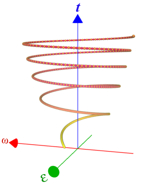
Figure 1: Typical control field $\omega\left({t}\right)$ and $\varepsilon\left({t}\right)$ as a function of time. Parameters correspond to the protocol of Fig. 3 Panel (d). Notice the change in frequency (chirp) and change in the generalized Rabi frequency $\Omega\left({t}\right)$.

The quality of the inertial approximation is directly connected to the parameter $\delta$. For small $|\delta|$, the inertial approximation is satisfied and the inertial solution remains accurate. The accuracy of the inertial solution can be evaluated by utilizing the time-dependent control protocol, Eq. (31). We choose the initial condition $\vec{v}\left({0}\right)=\{\hat{H}\left({0}\right),0,0,1\}$ which describes the system in the ground state ($\langle{\hat{H}\left({0}\right)}\rangle=-\Omega\left({0}\right)/2$). For these conditions, we compare the experimentally measured normalized energy, $\langle{\hat{H}\left({t}\right)}\rangle/\langle{\hat{H}\left({0}\right)}\rangle$, to the inertial solution, Eq. (26), and a converged numerical calculation of Eq. (4), which is generated by the Hamiltonian Eq. (10).

3 Experimental setup

The experimental analysis of the inertial solution employs a single Ytterbium ion ¹⁷¹Yb⁺, trapped in the six needles Paul trap, schematically shown in Fig. 2 Panel (a). The TLS (qubit) used in our study is encoded in the hyperfine energy levels of the ion, represented as ${\left|0\right>\equiv\,^{2}S_{1/2}\,\left|F=0,m_{F}=0\right>}$ and ${\left|1\right>\equiv\,^{2}S_{1/2}\,\left|F=1,m_{F}=0\right>}$, where $F$ denotes the total angular momentum of the atom and $m_{F}$ is its projection along the quantization axis. In absence of an external field, the subspace $F=1$ is degenerate. Therefore, we apply an external static magnetic field $\vec{B}$ with intensity $6.40$ G to obtain a $8.9$ MHz Zeeman structure splitting. This leads to the the desired TLS with a transition frequency given by $\omega_{hf}=2\pi\times 12.642~{}825$ GHz, see Fig. 2 Panel (b).

The TLS is controlled by a preprogrammed microwave, which is generated by mixing a $2\pi\times 12.442$  GHz coherent local oscillator microwave and a programmable Arbitrary Waveform Generator (AWG) signal, centered around $2\pi\times 200$ MHz [55, 56]. This enables implementing the components $\hat{\sigma}_{z}$ and $\hat{\sigma}_{x}$ of the Hamiltonian in Eq. (10), by simultaneous control of the microwave amplitude and the detuning between microwave frequency $\omega_{\mathbf{0}}$ and the transition frequency $\omega_{\mathbf{hf}}$ [55]. Here, the Rabi frequency $\varepsilon\left({t}\right)$ is directly proportional to the microwave amplitude, and $\omega_{\mathbf{0}}-\omega_{\mathbf{hf}}=\omega(t)$.

To initialize the experiment, first the motion of the ion is cooled by employing a $369.5$ nm Doppler cooling laser beam, using the optical transition cycle ${}^{2}S_{1/2}\!\rightleftarrows\!^{2}P_{1/2}$. During the transition cycle, there is a branching ratio $R$ for population decay from ${}^{2}P_{1/2}$ state to the ${}^{2}D_{3/2}$ [57]. To send the system back to the cooling cycle, a light at $935.2$ nm is used to promote transitions ${}^{2}D_{3/2}\!\rightleftarrows\!^{3}D[3/2]_{1/2}$, where the system can quickly decay from ${}^{3}D[3/2]_{1/2}$ to ${}^{2}S_{1/2}$ (grey arrows in Fig.  2 Panel (b)). After Doppler cooling, the system is initialized in the $\left|0\right>$ state with a standard optical pumping process. Utilizing the AWG, the time-frequency protocols of the inertial solutions are implemented.

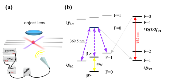
Figure 2: Experimental apparatus (a) and relevant Ytterbium energy levels (b) used in the experiment. The yellow color (waves and arrows) designates the RF transition, while the purple color signifies the doppler cooling laser transition. The grey arrow represent the spontaneous emission for the $P$ and $D$ manifolds, and the red color designates an additional optical transition, employed in order to close the cooling cycle. The qubit is encoded in the hyperfine states of the ${}^{2}S_{1/2}$. The readout is performed by fluorescence detection, utilizing the $395.5$ nm transition. where we highlight the encoding of the two-level system used in our experimental implementation.

The measurement procedure detects the population of the excited state of the qubit, using a fluorescence detection, induced by the $369.5$ nm laser [55, 56]. Thus, detection of photons correspond to population in the bright state $\left|1\right>$, while no photons signify population in the dark state $\left|0\right>$, as shown in Fig. 2,. The overall measurement fidelity is estimated to be $99.4\%$ [55, 58]. This experiment is repeated many times, for different delay times and different inertial protocols. For each experimental protocol, the normalized energy as a function of time is evaluated $\langle{\hat{H}\left({t}\right)}\rangle/\langle{\hat{H}\left({0}\right)}\rangle$.

4 Results

The qubit’s normalized energy as a function of time is shown in Figure 3, comparing the experimental measurements (blue) to the analytical inertial solution (red) and an exact numerical simulation (black). Experiments with different $\delta$ (Eq. (31)) were realized to asses the range of validity of the inertial solution. There is a good agreement between the theoretical and experimental results for small $\delta$ (see Panel (c) and (d)), demonstrating the high accuracy of the inertial solution. When $|\delta|=|d\mu/dt|$ is increased, we witness the breakdown of the inertial solution (Panels (a),(b),(e) and (f)), the deviations between the predicted normalized energy values of the inertial solution and the experimental results increase. The deviation is manifested by a difference in amplitude, while the phase of the inertial solution follows the exact simulation and experiment measurements, see Sec. 4.1 for a detailed analysis.

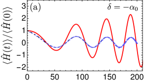
(a)

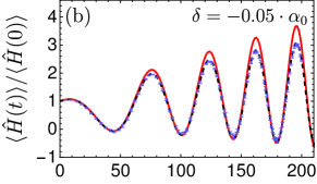
(b)

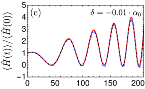
(c)

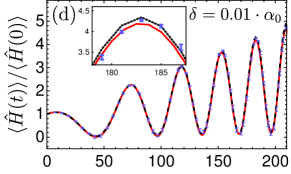
(d)

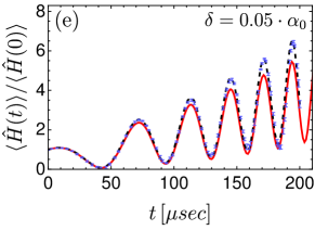
(e)

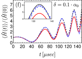
(f)

Figure 3: The normalized energy as a function of time for the experimental result (blue), inertial solution (red) and numerical solution (dashed-black) for different values of $\delta$: (a) $\delta=-\alpha\left({0}\right)$, (b) $\delta=-0.05\cdot\alpha\left({0}\right)$, (c) $\delta=-0.01\cdot\alpha\left({0}\right)$, (d) $\delta=0.01\cdot\alpha\left({0}\right)$, (e) $\delta=0.05\cdot\alpha\left({0}\right)$, (f) $\delta=0.1\cdot\alpha\left({0}\right)$. The experimental parameters are: $\alpha\left({0}\right)=6\cdot 2\pi KHz$, $\gamma=50\cdot 2\pi M(Hz)^{2}$ with $\mu\left({0}\right)=-1$. The varying values of $|\delta|=|d\mu/dt|$ are related to the quality of the inertial approximation; for slow change in $\mu$, the inertial approximation is satisfied (panels (c) and (d)). Varying $\mu$ rapidly leads to the breakdown of the inertial theorem (see Panels (a),(b),(e) and (f)). The insets in Panel (d) and (f) represent an enlarged section of the last oscillation, highlighting the experimental error bars.

Figure 4 shows the distance $\cal{D}$ between the inertial solution and the exact numerical result as a function of $\delta$ and time. $\cal{D}$ is defined as the Euclidean distance between the expectation values of the Liouville state vectors

$${\cal{D}}\left({t}\right)=\sqrt{\sum_{i=1}^{3}\left({\langle{v^{i}\left({t}\right)}\rangle-\langle{v_{num}^{i}\left({t}\right)}\rangle^{2}}\right)}~{}~{},$$ (32)

where $v_{i}$ and $v_{num}^{i}$ are the $i$’th component of $\vec{v}$ (the inertial solution) and $\vec{v}_{num}$ (the exact numerical solution). When $\mu$ varies slowly, ($\delta=-0.01$) the inertial solution remains exact, whereas for larger absolute values, the numerical and inertial solutions deviate linearly in $\delta$ and time. In Fig. 5, we present the inertial, numerical and adiabatic trajectories for $\delta=-0.01,-0.05$ in the $\langle{\hat{H}}\rangle,\langle{\hat{L}}\rangle,\langle{\hat{C}}\rangle$ space. This representation provides a complete description of the dynamics, demonstrating the large deviation between the adiabatic and inertial solutions.

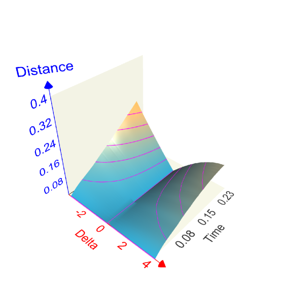
Figure 4: Distance ${\cal{D}}$ between the inertial solution and the exact numerical solution as a function of $\delta$ and time. For $\delta=0$, the inertial solution is exact at all times. For larger $|\delta|$, the distance increases almost linearly with time and $|\delta|$.

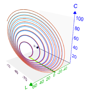
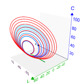
Figure 5: The inertial trajectory (red), exact numerical (blue) and adiabatic (green straight line) solutions in the $\langle{\hat{H}}\rangle,\langle{\hat{L}}\rangle,\langle{\hat{C}}\rangle$ coordinate space, for (a) $\delta=-0.01\cdot\alpha\left({0}\right)$ and (b) $\delta=-0.05\cdot\alpha\left({0}\right)$.

4.1 Deviations from the exact solution

There are two major sources of deviation between the inertial solution and experimental results. The first is associated with the breakdown of the inertial solution and the second source concerns the inevitable experimental noise. Observing Fig. 3 we find that the major deviation between the theoretical and experimental results is in the amplitude of the energy oscillations, while the phase is not affected even for large $|\delta|$ (see for example Panel (a) with $\delta=-\alpha\left({0}\right)$). The amplitude of the inertial solution is determined by the real part of the eigenvalues of the propagator. These are dominated by the the general scaling associated with the change in the generalized Rabi frequency, see Eq. (19). The imaginary part of the eigenvalues determine the phase.

In order to rationalize the observed deviation we first analyze the correction terms to the inertial solution. Gathering Eqs. (4), (15), and (19) we obtain

$$\frac{d\vec{u}^{H}\left({\theta}\right)}{d\theta}=-i{\cal{B}}^{\prime}\left({\mu\left({\theta}\right)}\right)\vec{u}^{H}\left({\theta}\right)~{}~{}.$$ (33)

Next, we define the instantaneous diagonalizing matrix of ${\cal{B}}^{\prime}\left({\mu}\right)$, satisfying ${\cal{P}}^{-1}\left({\mu}\right){\cal{B}}^{\prime}\left({\mu}\right){\cal{P}}\left({\mu}\right)={\cal{D}}\left({\mu}\right)$ and the vector $\vec{w}^{H}\left({\theta}\right)={\cal{P}}^{-1}\left({\mu}\right)\vec{u}^{H}\left({\theta}\right)$. The dynamics of $\vec{w}^{H}\left({\theta}\right)$ are given by

$$\frac{d\vec{w}\left({\theta}\right)}{d\theta}=-i{\cal{D}}\vec{w}\left({\theta}\right)+{\cal{O}}\vec{w}\left({\theta}\right)~{}~{},$$ (34)

where ${\cal{O}}=-{\cal{P}}^{-1}\frac{{\cal{P}}}{d\theta}$. For the studied model the diagonalizing matrix of ${\cal{B}}^{\prime}\left({\mu}\right)$, Eq. (17), obtains the form

$${\cal{P}}=\frac{1}{2\kappa^{2}}\left(\begin{array}[]{ccc}\frac{1}{\mu}&-\mu&-\mu\\ 0&i\kappa&-i\kappa\\ 1&1&1\end{array}\right)$$ (35)

For a slow change in $\mu$, ${\cal{B}}^{\prime}$ and consequently ${\cal{P}}$ vary slowly with respect to $\theta$. This property allows neglecting the second term in Eq. (34), which is qualitatively similar to the inertial approximation. The deviations from the exact solution are reflected by the term ${\cal{O}}\left({\theta}\right)={\cal{P}}^{-1}\frac{{\cal{P}}}{d\theta}$. Utilizing the identity $\frac{d{\cal{P}}}{d\theta}=\frac{1}{\Omega}\frac{d{\cal{P}}}{dt}$ we obtain

$${\cal{O}}=\frac{2\mu}{1+\mu^{2}}\frac{d\mu}{d\theta}{\cal{I}}+{\cal{S}}~{}~{},$$ (36)

where

$${\cal{S}}=\frac{\delta}{2\Omega\kappa^{2}}\left(\begin{array}[]{ccc}\frac{1}{\mu}&\mu&\mu\\ -\frac{1}{2\mu}&-\mu&0\\ -\frac{1}{2\mu}&0&-\mu\end{array}\right)~{}~{}.$$ (37)

Solving the dynamics explicitly leads to

$$\vec{w}\left({\theta}\right)=e^{\left({-i{\cal{D}+\cal{O}}}\right)\theta}\vec{w}\left({0}\right)~{}~{}~{}.$$ (38)

Next, we utilize the Zassenhaus formula [59] to obtain a solution up to first order in $\theta$

$$\vec{w}\left({\theta}\right)\approx e^{-i{\cal{D}}\theta}e^{{\cal{O}}\theta}\vec{w}\left({0}\right)~{}~{}~{}.$$ (39)

The correction term to the inertial solution has real eigenvalues, and therefore only influences the amplitude and not the phase. Thus, the phase of the inertial solution is not affected even when $|d\mu/dt|=|\delta|$ is large.

The second source of error is a consequence of experimental noise. We model this noise by a $\delta$-correlated noise in the timing of the driving [60]. Such a process is equivalent to adding random noise to the Generalized Rabi frequency $\Omega\left({t}\right)$, Eq. (13). In the presence of such a noise the effective equation of motion includes double commutator in the operator generating the noise [61]. For timing noise this becomes [62]:

$$\frac{d}{dt}\vec{v}^{H}\left({t}\right)=-\left[{{i{\cal{M}}\left({t}\right)}+\Gamma_{n}^{2}{\cal{M}}^{2}\left({t}\right)}\right]\vec{v}^{H}\left({t}\right)~{}~{},$$ (40)

where the double commutator is represented by ${\cal M}^{2}$, and $\Gamma_{n}$ is proportional to the noise amplitude. In this case, the noise has no effect on the eigenoperators with vanishing eigenvalues, $\hat{F}_{1}$ Eq. (25) (the time-dependent constants of motion). The other two eignvalues of the noise ${\cal{M}}^{2}\left({t}\right)$ are real and therefore will only influence the amplitude of the signal. The experimental results shown in Fig. 3 in particular the insert of Panel (d) and (f) corroborate this analysis.

5 Discussion

The purpose of this study was to establish experimentally a new family of inertial control protocols. These protocols are experimentally verified using a platform consisting of the hyperfine levels of an Ytterbium ion ¹⁷¹Yb⁺ in a Paul trap. This experimental platform is well suited for the evaluation due to its high fidelity. The high fidelity of both the control field and measurement allow direct comparison with the theoretical predictions. The inertial theorem provides a family of non-adiabatic protocols that bridge the gap between the sudden and adiabatic limits [43]. Specifically, we studied control of the $SU(2)$ Lie algebra, which constitutes the single qubit operations. We chose a protocol involving a chirp in frequency and change in the generalized Rabi frequency, associated with a linear change in the adiabatic parameter $\mu$.

The experiments verify the theorem and the ability to perform inertial protocols. Moreover, as all experiments are influenced by various kinds of noise [63], the achieved accuracy confirms the robustness of the inertial solution. This conclusion is supported by theoretical simulations which verify that the solution is stable to small deviations and noise.

For a larger deviation from the inertial condition ($d\vec{\chi}/dt\rightarrow 1$) (Fig. 3 panels (a), (b), (e) and (f)), the error first appears in the amplitude, while the phase of the inertial solution is still accurate. We confirm this by analyzing a correction to the inertial solution. In the $SU(2)$ algebra, the first-order correction in $\theta$ to the phase vanishes (see the discussion following Eq. 36). Incorporating the amplitude correction into the inertial solution can lead to higher accuracy. The phase information can be utilized for quantum parameter estimation [64] beyond the inertial limit.

Experimental validation of the inertial solution paves the way to rapid high-precision control. This control can be extended to inertially driven open systems [43], utilizing the non-adiabatic master equation [65]. Such control can regulate the system entropy [66, 67].

The present study constitutes a basic step in adding inertial control protocols to the family of constructive mechanisms of control. The experimental validation means that inertial protocols cross the barrier between a theoretical entity to laboratory use. Control based on the inertial theorem can be utilized in rapid applications of quantum information processing [68, 69, 70, 63] and sensing [71].

References

References

- [1] Steffen J Glaser, Ugo Boscain, Tommaso Calarco, Christiane P Koch, Walter Köckenberger, Ronnie Kosloff, Ilya Kuprov, Burkhard Luy, Sophie Schirmer, Thomas Schulte-Herbrüggen, et al. Training schrödinger’s cat: quantum optimal control. The European Physical Journal D, 69(12):1–24, 2015.
- [2] Juan I Cirac and Peter Zoller. Quantum computations with cold trapped ions. Physical review letters, 74(20):4091, 1995.
- [3] Chris Monroe, DM Meekhof, BE King, Wayne M Itano, and David J Wineland. Demonstration of a fundamental quantum logic gate. Physical review letters, 75(25):4714, 1995.
- [4] Julio T Barreiro, Markus Müller, Philipp Schindler, Daniel Nigg, Thomas Monz, Michael Chwalla, Markus Hennrich, Christian F Roos, Peter Zoller, and Rainer Blatt. An open-system quantum simulator with trapped ions. Nature, 470(7335):486, 2011.
- [5] S Rosi, A Bernard, Nicole Fabbri, Leonardo Fallani, Chiara Fort, Massimo Inguscio, Tommasco Calarco, and Simone Montangero. Fast closed-loop optimal control of ultracold atoms in an optical lattice. Physical Review A, 88(2):021601, 2013.
- [6] Olaf Mandel, Markus Greiner, Artur Widera, Tim Rom, Theodor W Hänsch, and Immanuel Bloch. Coherent transport of neutral atoms in spin-dependent optical lattice potentials. Physical review letters, 91(1):010407, 2003.
- [7] Immanuel Bloch, Jean Dalibard, and Wilhelm Zwerger. Many-body physics with ultracold gases. Reviews of modern physics, 80(3):885, 2008.
- [8] D Jaksch, JI Cirac, P Zoller, SL Rolston, R Côté, and MD Lukin. Fast quantum gates for neutral atoms. Physical Review Letters, 85(10):2208, 2000.
- [9] L-M Duan, Juan I Cirac, and Peter Zoller. Geometric manipulation of trapped ions for quantum computation. Science, 292(5522):1695–1697, 2001.
- [10] Daniel Jonathan, MB Plenio, and PL Knight. Fast quantum gates for cold trapped ions. Physical Review A, 62(4):042307, 2000.
- [11] Michael A Nielsen and Isaac Chuang. Quantum computation and quantum information, 2002.
- [12] Daniel Loss and David P DiVincenzo. Quantum computation with quantum dots. Physical Review A, 57(1):120, 1998.
- [13] Tadashi Kadowaki and Hidetoshi Nishimori. Quantum annealing in the transverse ising model. Physical Review E, 58(5):5355, 1998.
- [14] AB Finnila, MA Gomez, C Sebenik, C Stenson, and JD Doll. Quantum annealing: a new method for minimizing multidimensional functions. Chemical physics letters, 219(5-6):343–348, 1994.
- [15] J Brooke, D Bitko, G Aeppli, et al. Quantum annealing of a disordered magnet. Science, 284(5415):779–781, 1999.
- [16] Salvador E Venegas-Andraca, William Cruz-Santos, Catherine McGeoch, and Marco Lanzagorta. A cross-disciplinary introduction to quantum annealing-based algorithms. Contemporary Physics, 59(2):174–197, 2018.
- [17] Mark W Johnson, Mohammad HS Amin, Suzanne Gildert, Trevor Lanting, Firas Hamze, Neil Dickson, R Harris, Andrew J Berkley, Jan Johansson, Paul Bunyk, et al. Quantum annealing with manufactured spins. Nature, 473(7346):194, 2011.
- [18] Giuseppe E Santoro, Roman Martonak, Erio Tosatti, and Roberto Car. Theory of quantum annealing of an ising spin glass. Science, 295(5564):2427–2430, 2002.
- [19] Johannes Roßnagel, Samuel T Dawkins, Karl N Tolazzi, Obinna Abah, Eric Lutz, Ferdinand Schmidt-Kaler, and Kilian Singer. A single-atom heat engine. Science, 352(6283):325–329, 2016.
- [20] Jukka P Pekola. Towards quantum thermodynamics in electronic circuits. Nature Physics, 11(2):118, 2015.
- [21] Marcus W Doherty, Neil B Manson, Paul Delaney, Fedor Jelezko, Jörg Wrachtrup, and Lloyd CL Hollenberg. The nitrogen-vacancy colour centre in diamond. Physics Reports, 528(1):1–45, 2013.
- [22] MW Doherty, F Dolde, H Fedder, Fedor Jelezko, J Wrachtrup, NB Manson, and LCL Hollenberg. Theory of the ground-state spin of the nv- center in diamond. Physical Review B, 85(20):205203, 2012.
- [23] Nir Bar-Gill, Linh M Pham, Andrejs Jarmola, Dmitry Budker, and Ronald L Walsworth. Solid-state electronic spin coherence time approaching one second. Nature communications, 4:1743, 2013.
- [24] Hartmut Häffner, Christian F Roos, and Rainer Blatt. Quantum computing with trapped ions. Physics reports, 469(4):155–203, 2008.
- [25] David Kielpinski, Chris Monroe, and David J Wineland. Architecture for a large-scale ion-trap quantum computer. Nature, 417(6890):709, 2002.
- [26] Yuriy Makhlin, Gerd Schön, and Alexander Shnirman. Quantum-state engineering with josephson-junction devices. Reviews of modern physics, 73(2):357, 2001.
- [27] John M Martinis, S Nam, J Aumentado, and C Urbina. Rabi oscillations in a large josephson-junction qubit. Physical review letters, 89(11):117901, 2002.
- [28] Elisha Svetitsky, Haim Suchowski, Roy Resh, Yoni Shalibo, John M Martinis, and Nadav Katz. Hidden two-qubit dynamics of a four-level josephson circuit. Nature communications, 5:5617, 2014.
- [29] Christiane P Koch. Controlling open quantum systems: tools, achievements, and limitations. Journal of Physics: Condensed Matter, 28(21):213001, 2016.
- [30] Domenico d’Alessandro. Introduction to quantum control and dynamics. Chapman and Hall/CRC, 2007.
- [31] Constantin Brif, Raj Chakrabarti, and Herschel Rabitz. Control of quantum phenomena: past, present and future. New Journal of Physics, 12(7):075008, 2010.
- [32] Garng M Huang, Tzyh J Tarn, and John W Clark. On the controllability of quantum-mechanical systems. Journal of Mathematical Physics, 24(11):2608–2618, 1983.
- [33] Velimir Jurdjevic and Héctor J Sussmann. Control systems on lie groups. Journal of Differential equations, 12(2):313–329, 1972.
- [34] Viswanath Ramakrishna and Herschel Rabitz. Relation between quantum computing and quantum controllability. Physical Review A, 54(2):1715, 1996.
- [35] Ronnie Kosloff, Stuart A Rice, Pier Gaspard, Sam Tersigni, and DJ Tannor. Wavepacket dancing: Achieving chemical selectivity by shaping light pulses. Chemical Physics, 139(1):201–220, 1989.
- [36] Wusheng Zhu and Herschel Rabitz. A rapid monotonically convergent iteration algorithm for quantum optimal control over the expectation value of a positive definite operator. The Journal of Chemical Physics, 109(2):385–391, 1998.
- [37] José P Palao and Ronnie Kosloff. Quantum computing by an optimal control algorithm for unitary transformations. Physical review letters, 89(18):188301, 2002.
- [38] Shai Machnes, U Sander, Steffen J Glaser, P De Fouquières, A Gruslys, S Schirmer, and Thomas Schulte-Herbrüggen. Comparing, optimizing, and benchmarking quantum-control algorithms in a unifying programming framework. Physical Review A, 84(2):022305, 2011.
- [39] Nikolay V Vitanov, Andon A Rangelov, Bruce W Shore, and Klaas Bergmann. Stimulated raman adiabatic passage in physics, chemistry, and beyond. Reviews of Modern Physics, 89(1):015006, 2017.
- [40] Tameem Albash and Daniel A Lidar. Adiabatic quantum computation. Reviews of Modern Physics, 90(1):015002, 2018.
- [41] Max Born and Vladimir Fock. Beweis des adiabatensatzes. Zeitschrift für Physik, 51(3-4):165–180, 1928.
- [42] Daniel Comparat. General conditions for quantum adiabatic evolution. Physical Review A, 80(1):012106, 2009.
- [43] Roie Dann and Ronnie Kosloff. Inertial theorem: Overcoming the quantum adiabatic limit. Physical Review Research, 3(1):013064, 2021.
- [44] Leonard I Schiff. Quantum mechanics 3rd. New York: M cGraw-Hill, pages 61–62, 1968.
- [45] Lowell S Brown. Quantum motion in a paul trap. Physical review letters, 66(5):527, 1991.
- [46] Albert Messiah. Quantum mechanics 2 volumes, 2003.
- [47] Ali Mostafazadeh. Quantum adiabatic approximation and the geometric phase. Physical Review A, 55(3):1653, 1997.
- [48] MS Sarandy and DA Lidar. Adiabatic approximation in open quantum systems. Physical Review A, 71(1):012331, 2005.
- [49] Tosio Kato. On the adiabatic theorem of quantum mechanics. Journal of the Physical Society of Japan, 5(6):435–439, 1950.
- [50] Ugo Fano. Description of states in quantum mechanics by density matrix and operator techniques. Reviews of Modern Physics, 29(1):74, 1957.
- [51] John Von Neumann. Mathematical Foundations of Quantum Mechanics: New Edition. Princeton university press, 2018.
- [52] Robert Gilmore. Lie groups, Lie algebras, and some of their applications. Courier Corporation, 2012.
- [53] Y Alhassid and RD Levine. Connection between the maximal entropy and the scattering theoretic analyses of collision processes. Physical Review A, 18(1):89, 1978.
- [54] Roie Dann and Ronnie Kosloff. Thermodynamically consistent dynamics of driven open quantum systems: from an autonomous framework to the semi-classical description. arXiv preprint arXiv:2012.07979, 2020.
- [55] Chang-Kang Hu, Jin-Ming Cui, Alan C. Santos, Yun-Feng Huang, Marcelo S. Sarandy, Chuan-Feng Li, and Guang-Can Guo. Experimental implementation of generalized transitionless quantum driving. Opt. Lett., 43(13):3136–3139, Jul 2018.
- [56] Chang-Kang Hu, Jin-Ming Cui, Alan C. Santos, Yun-Feng Huang, Chuan-Feng Li, Guang-Can Guo, Frederico Brito, and Marcelo S. Sarandy. Validation of quantum adiabaticity through non-inertial frames and its trapped-ion realization. arXiv e-prints, page arXiv:1810.02644, 2018.
- [57] S. Olmschenk, K. C. Younge, D. L. Moehring, D. N. Matsukevich, P. Maunz, and C. Monroe. Manipulation and detection of a trapped hyperfine qubit. Phys. Rev. A, 76:052314, Nov 2007.
- [58] Chang-Kang Hu, Alan C Santos, Jin-Ming Cui, Yun-Feng Huang, Diogo O Soares-Pinto, Marcelo S Sarandy, Chuan-Feng Li, and Guang-Can Guo. Quantum thermodynamics in adiabatic open systems and its trapped-ion experimental realization. arXiv preprint arXiv:1902.01145, 2019.
- [59] Masuo Suzuki. Generalized trotter’s formula and systematic approximants of exponential operators and inner derivations with applications to many-body problems. Communications in Mathematical Physics, 51(2):183–190, 1976.
- [60] G. S. Agarwal. Quantum statistical theory of optical-resonance phenomena in fluctuating laser fields. Phys. Rev. A, 18:1490–1506, Oct 1978.
- [61] Vittorio Gorini, Andrzej Kossakowski, and Ennackal Chandy George Sudarshan. Completely positive dynamical semigroups of n-level systems. Journal of Mathematical Physics, 17(5):821–825, 1976.
- [62] Ronnie Kosloff and Tova Feldmann. Optimal performance of reciprocating demagnetization quantum refrigerators. Physical Review E, 82(1):011134, 2010.
- [63] Andrew M Childs, Edward Farhi, and John Preskill. Robustness of adiabatic quantum computation. Physical Review A, 65(1):012322, 2001.
- [64] Carl W Helstrom and Carl W Helstrom. Quantum detection and estimation theory, volume 84. Academic press New York, 1976.
- [65] Roie Dann, Amikam Levy, and Ronnie Kosloff. Time-dependent markovian quantum master equation. Phys. Rev. A, 98:052129, Nov 2018.
- [66] Roie Dann, Ander Tobalina, and Ronnie Kosloff. Shortcut to equilibration of an open quantum system. arXiv preprint arXiv:1812.08821, 2018.
- [67] Roie Dann, Ronnie Kosloff, and Peter Salamon. Quantum finite-time thermodynamics: insight from a single qubit engine. Entropy, 22(11):1255, 2020.
- [68] Dorit Aharonov, Wim Van Dam, Julia Kempe, Zeph Landau, Seth Lloyd, and Oded Regev. Adiabatic quantum computation is equivalent to standard quantum computation. SIAM review, 50(4):755–787, 2008.
- [69] Edward Farhi, Jeffrey Goldstone, Sam Gutmann, and Michael Sipser. Quantum computation by adiabatic evolution. arXiv preprint quant-ph/0001106, 2000.
- [70] Edward Farhi, Jeffrey Goldstone, Sam Gutmann, Joshua Lapan, Andrew Lundgren, and Daniel Preda. A quantum adiabatic evolution algorithm applied to random instances of an np-complete problem. Science, 292(5516):472–475, 2001.
- [71] Alejandro Perdomo-Ortiz, Joseph Fluegemann, Sriram Narasimhan, Rupak Biswas, and Vadim N Smelyanskiy. A quantum annealing approach for fault detection and diagnosis of graph-based systems. The European Physical Journal Special Topics, 224(1):131–148, 2015.