Gaussian Process Regression for Pricing Variable Annuities with Stochastic Volatility and Interest Rate

Abstract

In this paper we investigate price and Greeks computation of a Guaranteed Minimum Withdrawal Benefit (GMWB) Variable Annuity (VA) when both stochastic volatility and stochastic interest rate are considered together in the Heston Hull-White model. We consider a numerical method the solves the dynamic control problem due to the computing of the optimal withdrawal. Moreover, in order to speed up the computation, we employ Gaussian Process Regression (GPR). Starting from observed prices previously computed for some known combinations of model parameters, it is possible to approximate the whole price function on a defined domain. The regression algorithm consists of algorithm training and evaluation. The first step is the most time demanding, but it needs to be performed only once, while the latter is very fast and it requires to be performed only when predicting the target function. The developed method, as well as for the calculation of prices and Greeks, can also be employed to compute the no-arbitrage fee, which is a common practice in the Variable Annuities sector. Numerical experiments show that the accuracy of the values estimated by GPR is high with very low computational cost. Finally, we stress out that the analysis is carried out for a GMWB annuity but it could be generalized to other insurance products.

 

Keywords: GMWB pricing, Heston Hull-White model, Numerical method, Machine Learning, Gaussian Process Regression

 

1 Introduction

In this paper we focus on a particular Variable Annuity (VA) which leads the living benefit riders: the Guaranteed Minimum Withdrawal Benefit (GMWB). This contract is initiated by making a lump sum payment which is then invested in risky assets, usually a mutual fund. The holder of the policy (PH) is entitled to withdraw a fixed amount at the contract anniversaries, even if the risky account has declined to zero. If the amount withdrawn exceeds the guaranteed amount then a penalty is imposed. The contract also includes the payment of a benefit to the heirs of the PH in case of death during the coverage period. When the contract reaches maturity, a final payoff is paid out and the contract ends.

Researchers have engaged to develop new numerical techniques that are increasingly efficient and less computationally expensive. For example, Bacinello et al. [1] consider Monte Carlo methods to price and compute the Greeks of GMWB products. Chen and Forsyth [4] and Donnelly et al. [7] introduce partial derivative equations, while Costabile [5] propose pricing methods based on the use of trees. More recently, Goudenège et al. apply the Hybrid Tree-PDE method in order to compute the price and the Greeks of GLWB and GMWB contracts [12, 13]. However, as these techniques are more and more efficient, calculation times remain non-negligible, especially when the stochastic model considered to represent the market dynamics includes many random factors, such as stochastic volatility and stochastic interest rate. Moreover, the use of an accurate model that includes stochastic volatility and stochastic interest rate is crucial for treating products with long maturity, such as VAs in general.

In this paper, we investigate the evaluation of a GMWB contract when the Heston Hull-White model is considered. Such a stochastic model is particularly interesting since it provides for stochastic volatility and interest rate together. In particular, we consider the Hybrid Tree-PDE (HPDE) approach introduced by Briani et al. [3] which is a backward induction algorithm that works following a finite difference PDE method in the direction of the share process and a tree method in the direction of the other random sources, i.e. the stochastic volatility and the stochastic interest rate. Moreover, we develop a new trinomial tree to diffuse the additional random sources and we employ it to obtain an improved version of the HPDE method. Such a numerical method turns out to be particularly suitable to the scope of GMWB products since it is able to treat the long maturity of these insurance products. Moreover, since the PH can select the optimal amount to withdraw at each contract anniversary, a dynamic control problem must be solved and the HPDE method can be effectively applied to deal with this problem. In particular, we proceed backward in time by employing the HPDE method to compute the continuation value of the contract between two contract anniversaries and by modifying the contract state variables at each anniversary according to the optimal withdrawal strategy. To the best of our knowledge this is the first time that the GMWB has been priced in the Heston Hull-White model also considering an optimal withdrawal strategy.

The computations that insurance companies face depend on model parameters and contract parameters which are only few and vary in a small range. This context is similar to what happens in the derivatives world where there are many repeated valuations of standardized products. An innovative solution to speed up derivative pricing has been proposed by De Spiegeleer et al. [6], which consists in employing Machine Learning techniques to predict the price of the derivatives from a training set made of observed prices for particular combinations of model parameters. In particular, they consider Gaussian Process Regression (GPR) which is a Bayesian non-parametric technique. All the information needed to compute a function (the price or the Greeks of a derivative) can be summarized in a training set, then the algorithm learns the function and it can be applied to make predictions for new input parameters very fast. A similar approach, together with clustering techniques, has been employed by Gan [9] to price large portfolios of VAs in the Black-Scholes model. Unlike what De Spiegeleer et al. do, Gan considers fixed values for the market parameters (interest rate and volatility), having to repeat the procedure at each change in market conditions. Gan and Lin [10] propose a novel approach that combines clustering technique and GPR to efficiently evaluate policies considering nested simulations. More recently, Gan and Lin [11] propose a two-level metamodelling approach to efficiently estimating the sensitivities required to hedge a portfolio of VA, by employing GPR and Monte Carlo simulations.

As a second outcome, we show that Machine Learning techniques can be applied in the scope of GMWB products as far as pricing and Greeks calculation are considered in the Heston Hull-White model. In particular, we show that it is possible to develop a regression method capable of predicting the prices and the Greeks of each policy, for each combination of market and contract parameters within the training range. The training procedure requires the accurate calculation of the price and of the Greeks of a policy for different parameters configurations, which is done by the HPDE method. The training procedure needs to be performed only once and the developed regression can be applied under various market conditions and for different GMWB contracts. Moreover we also show that GPR can be applied effectively to compute the no-arbitrage fee, that is the cost that makes the contract fair under a risk neutral probability. Numerical tests show that the use of the GPR method reduces the computational time by several factors with a small loss of accuracy which makes the technique particularly interesting. Furthermore, unlike what proposed by Gan [9], no clustering technique for portfolios is required, providing and universal method that does not depends on specific template policies.

The main results of this paper consist in applying the HPDE method to appraising GMWB products and in speeding-up the evaluation by means of the GPR method so to obtain accurate evaluation of the policies in a very short time, what is required by all insurance companies. The reminder of the paper is organized as follows. In Section 2 we present the GMWB contract and we explain how to employ HPDE to compute prices and Greeks. In Section 3 we briefly review the GPR method and we explain how to apply it to the GMWB scope. In Section 4 we report the results of some numerical tests. Finally, Section 5 draws the conclusions.

2 The GMWB Contract and its Appraisal

In this Section we present the GMWB contract and the numerical method. Following Chen and Forsyth [4] and Goudenège et al. [13], we focus on a simplified version of the contract.

2.1 The GMWB Contract

At contract inception the PH pays, as a lump sum, the premium $P$ to the insurance company. Then, the PH is entitled to perform withdrawals at each contract anniversary, starting from $t=1$. In case of death of the insured, his heirs receive a benefit and the contact ends. If alive at maturity, the PH performs the last withdrawal, receives a final payoff and the contract ends. The contract evolution is described by two state parameters, the account value ($A_{t}$, $A_{0}=P$) and the base benefit ($B_{t}$, $B_{0}=P$), which change during the contract life according to the underlying fund value $S_{t}$ and to the PH withdrawals. Specifically, during the time between two consecutive contract anniversaries, the base benefit $B_{t}$ does not change, while the account value $A_{t}$ follows the same dynamics of $S_{t}$, with the exception that some fees, determined by the parameter $\alpha$, are subtracted from $A_{t}$ as follows:

$$dA_{t}=\frac{A_{t}}{S_{t}}dS_{t}-\alpha A_{t}dt.$$ (2.1)

During the contract anniversaries, the PH can withdraw from his account a minimum amount $G$ which is usually equal to $P/T$. Let us denote $A_{t_{i}^{\left(-\right)}},B_{t_{i}^{\left(-\right)}}$ the contract state variables just before the i-th contract anniversary occurs at time $t_{i}=i$, and $A_{t_{i}^{\left(+\right)}},B_{t_{i}^{\left(+\right)}}$ the same state variables just after $t_{i}$ occurs. Moreover, let $w_{i}$ represent the amount withdrawn at time $t_{i}$, which is required to be non-negative and smaller than the base benefit $B_{t_{i}^{\left(-\right)}}$. If the amount withdrawn satisfies $w_{i}\leq G$, then no penalty is imposed, whereas, if $w_{i}>G$, a proportional penalty charge $\kappa\left(w_{i}-G\right)$ reduces the amount actually received by the PH. To this aim, we denote with $f_{i}\left(w_{i}\right):\left[0,B_{t_{i}^{\left(-\right)}}\right]\rightarrow\mathbb{R}$ the net cash flow at time $t_{i}$:

$$f_{i}\left(W_{i}\right)=\begin{cases}w_{i}&\mbox{if }w_{i}\leq G\\ w_{i}-\kappa\left(w_{i}-G\right)&\mbox{if }w_{i}>G.\end{cases}$$

The contract state variables just after the withdrawal are updated as follows:

$$A_{t_{i}^{\left(+\right)}}=\max\left(A_{t_{i}^{\left(-\right)}}-w_{i},0\right),\text{ and }B_{t_{i}^{\left(+\right)}}=B_{t_{i}^{\left(-\right)}}-w_{i}.$$ (2.2)

If the PH passes away at time $\tau\in\left]t_{i-1},t_{i}\right[$, then his heirs receive a death benefit which is worth

$$DB=\max\left(A_{t_{i}^{\left(-\right)}},\left(1-\kappa\right)B_{t_{i}^{\left(-\right)}}\right)$$ (2.3)

and the contract ends. If the PH is alive at maturity time $T$, he is entitled to perform the last withdrawal and then he receives the final payoff which is worth

$$FP=\max\left(A_{T^{\left(+\right)}},\left(1-\kappa\right)B_{T^{\left(+\right)}}\right),$$ (2.4)

and the contract terminates. The effects of the mortality on the contract are described by means of two function: $\mathcal{M}:\left[0,T\right]\rightarrow\mathbb{R}$, which stands for the probability density of the random death year of the PH, and $\mathcal{R}:\left[0,T\right]\rightarrow\mathbb{R}$ that represents the fraction of the original owners who are still alive at time $t$, that is $\mathcal{R}\left(t\right)=1-\int_{0}^{t}\mathcal{M}\left(s\right)ds.$ For seek of simplicity, we assume $\mathcal{M}$ to be constant between contract anniversaries, and thus it can be easily obtained from a Mortality Table.

Let $\mathcal{V}\left(A,B,v,r,t_{i}^{\left(-\right)}\right)$, $\mathcal{V}\left(A,B,v,r,t_{i}^{\left(+\right)}\right)$ represent the contract value immediately before and after performing the withdrawal at time $t_{i}$, respectively. Following Forsyth and Vetzal [8], we consider the worst withdrawal strategy for the insurer, that is

$$w_{i}=\underset{w\in\left[0,B_{t_{i}^{\left(-\right)}}\right]}{\mbox{argmax}}\ \mathcal{V}\left(\max\left(A_{t_{i}^{\left(-\right)}}-w,0\right),B_{t_{i}^{\left(-\right)}}-w,v_{t_{i}},r_{t_{i}},t_{i}^{\left(+\right)}\right)+\mathcal{R}\left(t_{i}\right)f_{i}\left(w\right).$$ (2.5)

Assuming such a strategy and hedging against it is clearly very conservative, but it ensures no losses for the insurance company.

2.2 The Stochastic Model for the Underlying and the GMWB Appraisal

The Heston Hull-White model includes both stochastic volatility and stochastic interest rate as follows:

$$\begin{cases}dS_{t}&=r_{t}S_{t}dt+\sqrt{v_{t}}S_{t}dZ_{t}\\ dv_{t}&=k_{v}\left(\theta_{v}-v_{t}\right)dt+\omega_{v}\sqrt{v_{t}}dW_{t}^{v},\\ dr_{t}&=k_{r}\left(\theta_{r}\left(t\right)-r_{t}\right)dt+\omega_{r}dW_{t}^{r},\end{cases}$$ (2.6)

where $Z$, $W^{v}$ and $W^{r}$ are Brownian motions such that $d\left\langle Z_{t},W_{t}^{v}\right\rangle=\rho_{v}dt$, $d\left\langle Z_{t},W_{t}^{r}\right\rangle=\rho_{r}dt$ and $d\left\langle W_{t}^{v},W_{t}^{r}\right\rangle=0$. Here $\theta_{r}\left(t\right)$ is a deterministic function which is completely determined by the market values of the zero-coupon bonds by calibration. For seek of simplicity, we assume that the market price of a zero-coupon bond at time $t$ with maturity $\bar{t}$ is given by $P^{M}\left(t,\bar{t}\right)=e^{-r_{0}\left(\bar{t}-t\right)}$, the so-called flat curve case.

The parameters which identify the Heston Hull-White model are the initial volatility $v_{0}$, the rate of mean reversion $k_{v}$, the long run variance $\theta_{v}$, the volatility of volatility $\omega_{v}$, the correlation $\rho_{v}$, the initial interest rate $r_{0}$, the rate of mean reversion $k_{r}$, the volatility of the interest rate $\omega_{r}$ and the correlation $\rho_{r}$. In order to compute the fair price and the Greeks of a GMWB contract in the Heston Hull-White model, we apply the HPDE method, introduced by Briani et al. [3] for option pricing and successfully employed in the framework of VAs by Goudenège et al. [12, 13] while considering the Heston and the Black-Scholes Hull-White models. The HPDE is a backward induction algorithm that works following a finite difference PDE method in the direction of the share process and following a tree method in the direction of the volatility and of the interest rate. We give here some details about the numerical method and we refer the interested reader to [2, 3, 12, 13] for a detailed description. We start by observing that $r$ can be written as

$$r_{t}=\omega_{r}x_{t}+\varphi_{t},$$ (2.7)

where

$$x_{t}=-k_{r}\int_{0}^{t}x_{t}ds+W_{t}^{r}\ \text{ and }\ \varphi_{t}=r_{0}e^{-k_{r}t}+k_{r}\int_{0}^{t}\theta_{r}\left(s\right)e^{-k_{r}\left(t-s\right)}ds.$$ (2.8)

We consider now an approximating tree $\left(\hat{v}_{n}^{h}\right)_{n\in\left\{0,\dots,N\right\}}$ for $v$ and $\left(\hat{x}_{n}^{h}\right)_{n\in\left\{0,\dots,N\right\}}$ for $x$, both with $N$ time-steps. Since the GMWB contract are long maturity contracts (up to $30$ years), the binomial trees proposed in [3] are not suitable in this context. In the Appendix A we report how to obtain trinomial trees that are more suitable for the scope of VAs. These tree are a good compromise between precision and required working memory. So, let $\Delta t=\frac{T}{N}$ and $t_{n}=n\Delta t$. We proceed backward along the tree and at each time $t_{n}$, for each couple of nodes $\left(\hat{v}_{n}^{h},\hat{x}_{n}^{h}\right)$, we consider the values of $v_{t}$ and $x_{t}$ equal to $\hat{v}_{n}^{h}$ and $\hat{x}_{n}^{h}$ respectively. Then, we compute the contract value at time $t_{n}$ for each value of $B$ as the solution of a one-dimensional partial derivative equation that depends on a suitable transformation $z$ of the account value $A$ (see Briani et al [3]):

$$\begin{cases}\partial_{t}u+\mu\left(v,x,t\right)\partial_{z}u+\frac{1}{2}\rho_{3}^{2}v\partial_{z}^{2}u&=0\\ u\left(t_{i+1},z;v,x\right)&=\mathcal{V}\left(A\left(z\right),B,v,\omega_{r}x+\varphi_{t},t_{i+1}^{-}\right)\end{cases}$$ (2.9)

The solution of such a PDE is computed at each tree node by performing a finite difference step.

3 Gaussian Process Regression for GMWB

In this Section, we present a brief review of the Gaussian Process Regression and for a comprehensive treatment we refer to Rasmussen and Williams [16]. GPR is a class of non-parametric kernel-based probabilistic models which represents the input data as the random observations of a Gaussian stochastic process. In a nutshell, the GPR technique is used to make extrapolations in high dimension. The most important advantage of this approach is that it is possible to effectively exploit a complex dataset which may consist of points sampled randomly in a multidimensional space. This is particularly useful when the domain dimension is high, in which case even the mere construction of a grid of points requires a prohibitive computational effort. Finally, compared to other artificial intelligence techniques such as neural networks, GPR requires less computational time and less input data to produce accurate results.

3.1 Gaussian Process Regression

Let $X=\left\{\mathbf{x}_{i}\right\}_{i=1,\dots,n}\subset\mathbb{R}^{D}$ be the set of predictors and $Y=\left\{y_{i}\right\}_{i=1,\dots,n}\subset\mathbb{R}$ the set of scalar outputs. These observations are modeled as the realization of the sum of a Gaussian process $\mathcal{G}$ and a Gaussian noise source $\varepsilon$. In particular, the distribution of $\mathbf{y}=\left(y_{1}\dots y_{n}\right)$ is assumed to be given by

$$\mathbf{y}\sim\mathcal{N}\left(\mu\left(X\right),K\left(X,X\right)+\sigma_{n}^{2}I_{n}\right),$$ (3.1)

with $\mu$ the mean function, $I_{n}$ the $n\times n$ identity matrix and $K$ a $n\times n$ matrix given by $K\left(X,X\right)_{i,j}=k\left(\mathbf{x}_{i},\mathbf{x}_{j}\right)$. Here, we consider the Automatic Relevance Determination Squared Exponential (ARD SE) kernel, which is given by

$$k\left(\mathbf{x},\mathbf{x}^{\prime}\right)=\sigma_{f}^{2}\exp\left(-\frac{1}{2}\sum_{k=1}^{D}\frac{1}{l_{k}^{2}}\left(x_{k}-x_{k}^{\prime}\right)^{2}\right),$$ (3.2)

where $\sigma_{f}^{2}$ is the signal variance and $l_{k}$ is the length-scale along the $k$ direction.

Now, in addition, let us consider a test set $\tilde{X}$ of $m$ points $\left\{\tilde{\mathbf{x}}_{j}|j=1,\dots,m\right\}$. The realizations $\tilde{f}_{j}=\mathcal{G}\left(\tilde{\mathbf{x}}_{j}\right)+\varepsilon_{j}$ are not known but are predicted through $\mathbb{E}\left[\mathbf{\tilde{f}}|\tilde{X},\mathbf{y},X\right]$:

$$\mathbb{E}\left[\mathbf{\tilde{f}}|\tilde{X},\mathbf{y},X\right] =\mu\left(\tilde{X}\right)+K\left(\tilde{X},X\right)A,$$ (3.3)

with $A=\left[K\left(X,X\right)+\sigma_{n}^{2}I_{n}\right]^{-1}\left(\mathbf{y}-\mu\left(X\right)\right)$. The mean function $\mu$, which is assumed to be a linear function of the predictors, is determined analytically by multi-linear regression. The parameters $\sigma_{f}^{2}$, $l_{1},\dots,l_{D}$ of the kernel and $\sigma_{n}^{2}$ of the noise are termed hyperparameters and they are estimated by log-likelihood maximization.

The development of the GPR method consists in two steps: training and evaluation (also called testing). The former consists in estimating $\mu$, the hyperparameters and computing $A$ while the latter can be performed only after the training and it consists in obtaining the predictions via (3.3).

3.2 Applying the GPR to the GMWB Contract

We aim to apply the GPR method to GMWB products to speed up the computation of the price and of the Greeks. The modeling process starts by computing a training set $\mathcal{D}$. The predictor set $X$ consists of $n$ combinations of the stochastic model and GMWB product parameters. Specifically, the predictors are $v_{0}$, $k_{v}$, $\theta_{v}$, $\omega_{v}$, $\rho_{v}$, $r_{0}$, $k_{r}$, $\omega_{r}$, $\rho_{r}$ $\alpha$ and $\kappa$. We accentuate that we can avoid considering the premium $P$ as a predictor since the price $\mathcal{V}$ of the GMWB contract is directly proportional to $P,$ that is $\mathcal{V}/P$ does not depend on $P$. Similarly Greeks can be obtained from the Greeks computed for a particular value of $P$: for example, Delta does not depend on the considered value of $P$. Moreover we do not consider the contract maturity among the predictors since this is a discrete parameter which usually varies in a small set (usually $T=5,10$ or $20$) and one can compute an independent GPR for each value of $T$. Pseudo-random combinations are sampled uniformly over a fixed range for each parameter. Specifically, $n$ parameters combinations are sampled through the Faure sequence which covers efficiently all the domain of the parameters and yields better results than a random sample. For each parameter combination, we compute the price and then, observed data are passed to the GPR algorithm. Once the training step is finished, the model is ready to estimate prices. The same can be done for the Greeks. We point out that the procedure described above relates to the valuation of a single policy. If a portfolio of policies is considered instead, pricing and sensitivity calculation can be done for each contract individually. The no-arbitrage fee $\alpha_{na}$ of a GMWB contract is the particular value of $\alpha$ which makes the initial value of the policy $\mathcal{V}\left(P,P,v_{0},r_{0},0\right)$ equal to the premium $P$ and its computation is a common practice before the sale of a contract. This value is usually determined by employing the secant method, seeking to equate $\mathcal{V}\left(P,P,v_{0},r_{0},0\right)$ and $P$. The GPR method can be applied within the secant method to boost the computation of $\alpha_{na}$ by replacing the direct computation of $\mathcal{V}\left(P,P,v_{0},r_{0},0\right)$ with HPDE by the GPR prediction.

4 Numerical Results

In this Section we report some numerical results. Specifically, in the first test we show the accuracy of the Hybrid Tree-PDE algorithm in pricing and in computing Delta and the no-arbitrage fees. Then, in the following two tests, we apply the GPR method to predict the no-arbitrage fee and the Greek $\Delta$ of a GMWB contract respectively. The HPDE algorithm has been implemented in C++, whereas the regression algorithm has been implemented in MATLAB and computations have been performed on a PC equipped with $8$ GB of RAM and a 2.5GHz i5-7200u processor. The performance of the GPR mehtod is measured in terms of the following indicators which depend on the maximum and average absolute and relative error: the RMSE (Root Mean Squared Error), the RMSRE (Root Mean Squared Relative Error), the MaxAE (Maximum Absolute Error) and the MaxRE (Maximum Relative Error). Finally, we also report the speed-up that is the ratio between the computational time achieved with a direct computation by HPDE and the computational time achieved by using the GPR method.

4.1 Testing the HPDE method

We show the accuracy of the HPDE method which is involved in the computation of the data employed in both the training and testing steps. Input parameters are reported in Table 1 while results are available in Table 2. Moreover, the DAV 2004R mortality Table for a 65 year old German male is employed to compute the functions $\mathcal{M}$ and $\mathcal{R}$ (see Forsyth and Vetzal [8] for the Table). Specifically, we compute the price, the Delta and the no-arbitrage fee considering several configurations with increasing number of time and space steps (see Goudenège et al. [12, 13] for further details). Numerical results suggested that a few steps is enough to obtain accurate values but, the computational times may become considerable.

Name	Symbol	Value		Name	Symbol	Value
Premium	$P$	$100$		Initial interest rate	$r_{0}$	$0.02$
Maturity	$T$	$10$ years		Rate of mean reversion	$k_{r}$	$0.15$
Initial volatility	$v_{0}$	$0.05$		Volatility of interest rate	$\omega_{r}$	$0.015$
Rate of mean reversion	$k_{v}$	$2.00$		Correlation	$\rho_{r}$	$0.20$
Long run variance	$\theta_{v}$	$0.05$		Fees	$\alpha$	$0.035$
Volatility of volatility	$\omega_{v}$	$0.50$		Penalty	$\kappa$	$0.10$
Correlation	$\rho_{v}$	$-0.55\phantom{-}$

Table 1: The parameters employed.

Time and space steps	$125\times 125$	$250\times 250$	$500\times 500$	$1000\times 1000$
Price	$\underset{\left(7.8\text{e}+0\right)}{100.08}$	$\underset{\left(8.3\text{e}+1\right)}{100.11}$	$\underset{\left(1.1\text{e}+3\right)}{100.12}$	$\underset{\left(1.4\text{e}+4\right)}{100.12}$
Delta	$\underset{\left(7.8\text{e}+0\right)}{0.3881}$	$\underset{\left(8.3\text{e}+1\right)}{0.3888}$	$\underset{\left(1.1\text{e}+3\right)}{0.3892}$	$\underset{\left(1.4\text{e}+4\right)}{0.3894}$
No-arbitrage fee	$\underset{\left(4.6\text{e}+1\right)}{353.45}$	$\underset{\left(5.0\text{e}+2\right)}{354.81}$	$\underset{\left(6.6\text{e}+3\right)}{355.25}$	$\underset{\left(8.4\text{e}+4\right)}{355.55}$

Table 2: Hybrid Tree-PDE computation results. The values in brackets are the computational times measured in seconds. The no-arbitrage fee is expressed in bps.

4.2 No-arbitrage Fee Results

We test the ability of the GPR model to compute the no-arbitrage fee of a GMWB contract. Table 3 report the ranges for the input parameters. The training set consists of $n=1250,$ $2500$, $5000$, $10000$, or $20000$ combinations of parameters and the prices obtained by using the HPDE method with $250$ time and space steps. The regression model is tested on both input data and out-of-sample data. In particular, out-of-sample data consists of $m=20000$ additional parameters combinations which are obtained by a random simulation. Numerical results are reported in Table 4. The scatter plot of out-of-sample absolute errors for a model trained on $n=10000$ data is shown in Figure 4.1a. Specifically, prediction errors are sorted according to the respective policy price and we can see that the errors remain in an admissible band.

Name	Symbol	Value		Name	Symbol	Value
Premium	$P$	$100$		Initial interest rate	$r_{0}$	$\left[0.01,0.03\right]$
Maturity	$T$	$10$ years		Rate of mean reversion	$k_{r}$	$\left[0.05,0.25\right]$
Initial volatility	$v_{0}$	$\left[0.01,0.10\right]$		Volatility of interest rate	$\omega_{r}$	$\left[0.005,0.025\right]$
Rate of mean reversion	$k_{v}$	$\left[1.40,2.60\right]$		Correlation	$\rho_{r}$	$\left[0.05,0.35\right]$
Long run variance	$\theta_{v}$	$\left[0.01,0.10\right]$		Fees	$\alpha$	$\left[0.00,0.10\right]$
Volatility of volatility	$\omega_{v}$	$\left[0.45,0.75\right]$		Penalty	$\kappa$	$\left[0.00,0.20\right]$
Correlation	$\rho_{v}$	$\left[\text{\^{A}\-}-0.70,-0.40\right]$

Table 3: The range of the parameters.

Size of training set	1250	2500	5000	10000	20000
RMSE	7.88e-4	5.94e-4	4.82e-4	3.93e-4	3.74e-4
RMSRE	2.30e-2	1.98e-2	1.54e-2	1.36e-2	1.20e-2
MaxAE	2.02e-2	1.08e-2	8.10e-3	6.50e-3	6.13e-3
MaxRE	3.22e-1	3.07e-1	2.74e-1	1.66e-1	1.51e-1
Speed-up	$\times$9.8e5	$\times$3.8e5	$\times$1.8e5	$\times$1.2e5	$\times$6.4e4

Table 4: Performances of the GPR method in computing the no-arbitrage fee.

4.3 Delta Results

We test the ability of the GPR model to predict the first derivative Delta of a GMWB contract, which is crucial in hedging. Numerical results are reported in Table 5, while the scatter plot of the estimation errors is shown in Figure 4.1b. In particular, errors are distributed around zero with any evident outline.

Size of training set		1250	2500	5000	10000	20000
	RMSE	1.94e-4	6.09e-4	6.93e-4	8.16e-4	9.37e-4
In-sample	RMSRE	8.28e-4	3.75e-3	3.95e-3	5.16e-3	6.07e-3
prediction	MaxAE	8.84e-4	3.95e-3	6.30e-3	7.78e-3	1.60e-2
	MaxRE	7.47e-3	9.42e-2	1.08e-1	1.64e-1	2.52e-1
	RMSE	2.65e-3	1.88e-3	1.44e-3	1.22e-3	1.16e-3
Out-of-sample	RMSRE	1.83e-2	1.20e-2	8.97e-3	7.78e-3	7.39e-3
prediction	MaxAE	3.26e-2	2.70e-2	2.47e-2	1.87e-2	2.10e-2
	MaxRE	6.25e-1	4.26e-1	2.64e-1	2.63e-1	2.50e-1
Speed-up		$\times$9.8e5	$\times$3.8e5	$\times$1.8e5	$\times$1.2e5	$\times$6.4e4

Table 5: Performances of the GPR method in computing Delta.

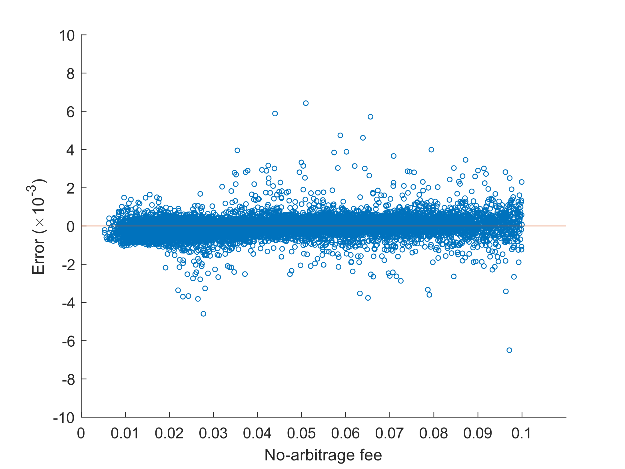
(a) No-arbitrage fee

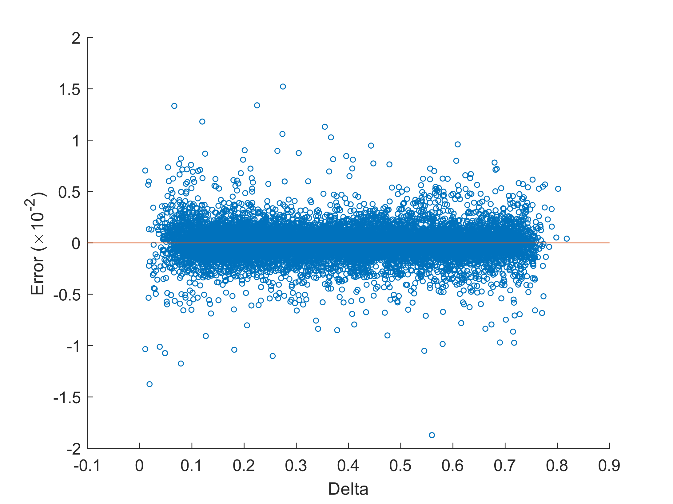
(b) Delta

Figure 4.1: Out-of-sample prediction absolute errors for a GPR method trained on $n=10000$ points.

4.4 Remarks on Computational Results

Tables 4 and 5 show the performance of the developed approach. Errors are very small in all the considered cases, indicating that the predictions are very accurate. The most interesting aspect is the gain in terms of computation time: it is reduced by thousands of times. Moreover, Table 6 shows the computational time for the training step. The cost of the training step depends on both the size of the training set, and the target function (price or Delta). We observe that the required time is high when the size of the training set is $n=20000$ because in this case the BCD algorithm is used in place of the exact computation (see Grippo and Sciandrone [14]). Finally, Table 7 shows the predicted price, Delta and no-arbitrage fee for the same GMWB policy considered in Table 2. We observe that the estimates are very accurate and the gain in terms of computational time is considerable.

Size of training set	1250	2500	5000	10000	20000
Price	49	154	185	188	3219
Delta	32	110	128	142	3144

Table 6: The computational time (in seconds) to train the GPR algorithm.

Size of training set	1250	2500	5000	10000	20000
Price	$\underset{\left(8.5\text{e}-5\right)}{100.10}$	$\underset{\left(2.2\text{e}-4\right)}{100.09}$	$\underset{\left(4.6\text{e}-4\right)}{100.09}$	$\underset{\left(6.8\text{e}-4\right)}{100.09}$	$\underset{\left(1.3\text{e}-3\right)}{100.09}$
Delta	$\underset{\left(8.4\text{e}-5\right)}{0.3899}$	$\underset{\left(1.9\text{e}-4\right)}{0.3892}$	$\underset{\left(4.2\text{e}-4\right)}{0.3892}$	$\underset{\left(7.4\text{e}-4\right)}{0.3891}$	$\underset{\left(1.4\text{e}-3\right)}{0.3891}$
No-arbitrage fee	$\underset{\left(5.1\text{e}-4\right)}{354.27}$	$\underset{\left(1.3\text{e}-3\right)}{354.08}$	$\underset{\left(2.8\text{e}-3\right)}{353.93}$	$\underset{\left(4.1\text{e}-3\right)}{354.01}$	$\underset{\left(7.8\text{e}-3\right)}{354.03}$

Table 7: GPR computation results. The values in brackets are the computational times measured in seconds. The no-arbitrage fee is expressed in bps.

5 Conclusions

In this paper we have presented how Gaussian Process Regression can be applied in the insurance field to address the problem of pricing and computing the sensitivities of a GMWB Variable Annuity when both stochastic volatility and stochastic interest rate are considered. The HPDE method proves to be an effective tool for calculating prices and Greeks in the Heston Hull-White model, however it may be time demanding if a large number of time-steps is considered. The GPR method allows one to considerably reduce the computational time as the greater computational effort is carried out during the training phase, which must be performed only once before the actual use of the model while computing a single prediction. The use of a pseudo-random method and of a general kernel allow one to obtain accurate results with a small amount of observations. The resulting model can be applied to compute the prices of the policies, for hedging purposes, or to compute the no-arbitrage cost of a policy and can be particularly useful in the case of books of policies, when the evaluation must be repeated many times. We conclude observing that the same approach may be applied to all types of Variable Annuities contracts.

Appendix A The Trinomial Tree

In this Appendix we present how to build a trinomial tree for the volatility process $v$ and the interest rate process $x$. In the scope of pricing long maturity products, the trinomial tree proposed here turns out to be more suitable of the binomial tree proposed by Briani et al. [3] since it matches exactly the first two moments of the developed process and convergence is faster. Let $Z$ be a Brownian motion and let $G$ be a Gaussian process, given by

$$dG_{t}=a\left(G_{t}\right)dt+bdZ_{t},$$ (A.1)

with variance that depends only by the time lapse, i.e. $G_{t+h}|\mathcal{F}_{t}\sim\mathcal{N}\left(\mu\left(h,G_{t}\right),\sigma^{2}\left(h\right)\right)$ where $\mu\left(h,G_{t}\right)$ and $\sigma^{2}\left(h\right)$ are respectively the expectation and the variance of the of the process $G$.

We show how to build a simple trinomial tree that can match the first two moments of $G$. Let’s fix a maturity $T$ a number of time-steps $N$ and setfine $\Delta t=\nicefrac{{T}}{{N}}$. Each node will be denoted by $G_{n,j}$ where $n\in\left\{0,\dots,N\right\}$ and $j\in\left\{0,\dots,2n\right\}$ . The value of each node is

$$G_{n,j}=G_{0}+\frac{3}{2}\left(j-n\right)\sqrt{\sigma^{2}\left(\Delta t\right)}.$$ (A.2)

We recall the first two moments $\left(M_{1},M_{2}\right)$ of the process $G$:

$$M_{1}\left(\Delta t,G_{t}\right)=\mathbb{E}\left[G_{t+\Delta t}|\mathcal{F}_{t}\right]=\mu\left(\Delta t,G_{t}\right),\ M_{2}\left(\Delta t,G_{t}\right)=\mathbb{E}\left[\left(G_{t+\Delta t}\right)^{2}|\mathcal{F}_{t}\right]=\mu^{2}\left(\Delta t,G_{t}\right)+\sigma^{2}\left(\Delta t\right).$$ (A.3)

Let’s fix a node $G_{n,j}$. To be brief, $\mu$ will denote $\mu\left(\Delta t,G_{n,j}\right)$ and $\sigma$ will denote $\sqrt{\sigma^{2}\left(\Delta t\right)}$. We suppose that the conditional expected value $\mu=\mathbb{E}\left[G_{t+h}|\mathcal{F}_{t}\right]$ falls between the values of the nodes at time $\left(n+1\right)\Delta t$. This hypothesis can be justify assuming that the time increment $\Delta t$ is small enough (in fact, by continuity, $\lim_{\Delta t\rightarrow 0^{+}}\mu\left(\Delta t,G_{n,j}\right)=G_{n,j}$ which is a node). We define

$$j_{A}\left(n,j\right)=n+\mbox{ceil}\left[\frac{2}{3\sigma}\left(\mu-G_{0}\right)\right],$$ (A.4)

i.e. the first node whose value is bigger than the mean of the process. Let

$$j_{B}\left(n,j\right)=j_{A}\left(n,j\right)-1,\ j_{C}\left(n,j\right)=j_{A}\left(n,j\right)+1,\ j_{D}\left(n,j\right)=j_{A}\left(n,j\right)-2.$$ (A.5)

To be brief we will only write $j_{A},j_{B},j_{C},$ $j_{D}$, and $G_{A}$ will be $G_{A}=G_{n+1,j_{A}}$ and the same for the other letters. We can now define a Markovian discrete time process $\hat{G}_{n}$, $n=0,\dots,N$ with $\hat{G}_{0}=G_{0,0}$. Let $\hat{G}_{n}=G_{n,j}$. If $0\leq G_{A}-\mu\leq\frac{3}{4}\sigma$ then $\hat{G}_{n}$ can move to $G_{A}$, $G_{B}$, $G_{C}$, otherwise $\hat{G}_{n}$ can move to $G_{A}$, $G_{B}$, $G_{D}$. Transition probabilities are stated in Table 8.

	if $0\leq G_{A}-\mu\leq\frac{3}{4}\sigma$	if $\frac{3}{4}\sigma<G_{A}-\mu$
$p_{A}$	$\frac{5\sigma^{2}-4\left(G_{A}-\mu\right)^{2}}{9\sigma^{2}}$	$\frac{2\left(\mu-G_{B}\right)^{2}+3\sigma\left(\mu-G_{B}\right)+2\sigma^{2}}{9\sigma^{2}}$
$p_{B}$	$\frac{2\left(G_{A}-\mu\right)^{2}+3\sigma\left(G_{A}-\mu\right)+2\sigma^{2}}{9\sigma^{2}}$	$\frac{5\sigma^{2}-4\left(\mu-G_{B}\right)^{2}}{9\sigma^{2}}$
$p_{C}$	$\frac{2\left(G_{A}-\mu\right)^{2}-3\sigma\left(G_{A}-\mu\right)+2\sigma^{2}}{9\sigma^{2}}$	$0$
$p_{D}$	$0$	$\frac{2\left(\mu-G_{B}\right)^{2}-3\sigma\left(\mu-G_{B}\right)+2\sigma^{2}}{9\sigma^{2}}$

Table 8: Transition probabilities for the trinomial tree.

Since $G_{B}<\mu\leq G_{A}$, we can easily show that these probabilities are well defined: all in $\left[0,1\right]$, their sum is equal to $1$, and the first two moments of the variable $\hat{G}_{n+1}|\hat{G}_{n}=G_{n,j}$ are equal to the first two moments of the variable $G_{t+h}|G_{t}=G_{n,j}$.

We can approximate the process $G$ by a process $\bar{G}$ that is constant in each time lapse and is defined by $\bar{G}_{t}=\hat{G}_{\left\lfloor\nicefrac{{t}}{{h}}\right\rfloor}$. The weak convergence of this tree can be proved as in Nelson and Ramaswamy [15].

This construction can be directly applied to build a tree for the process $x$ since it is Gaussian. As far as the volatility process is concerned, this method cannot be directly applied since $v$ has no constant variance and is not Gaussian. However, it can be easily be modified as in [12], so as to guarantee the week convergence.

References

- [1] A. R. Bacinello, P. Millossovich, A. Olivieri, and E. Pitacco. Variable Annuities: A unifying valuation approach. Insurance: Mathematics and Economics, 49(3):285–297, 2011.
- [2] M. Briani, L. Caramellino, and A. Zanette. A hybrid approach for the implementation of the Heston model. IMA Journal of Management Mathematics, 28(4):467–500, 2017.
- [3] M. Briani, L. Caramellino, and A. Zanette. A hybrid tree/finite-difference approach for Heston–Hull–White-type models. Journal of Computational Finance, 21(3), 2017.
- [4] Z. Chen and P. A. Forsyth. A numerical scheme for the impulse control formulation for pricing Variable Annuities with a Guaranteed Minimum Withdrawal Benefit (GMWB). Numerische Mathematik, 109(4):535–569, 2008.
- [5] M. Costabile. A lattice-based model to evaluate Variable Annuities with Guaranteed Minimum Withdrawal Benefits under a regime-switching model. Scandinavian Actuarial Journal, 2017(3):231–244, 2017.
- [6] J. De Spiegeleer, D. B. Madan, S. Reyners, and W. Schoutens. Machine learning for quantitative finance: fast derivative pricing, hedging and fitting. Quantitative Finance, 18(10):1635–1643, 2018.
- [7] R. F. Donnelly, S. Jaimungal, and D. Rubisov. Valuing guaranteed withdrawal benefits with stochastic interest rates and volatility. Quantitative Finance, 14(2):369–382, 2014.
- [8] P. Forsyth and K. Vetzal. An optimal stochastic control framework for determining the cost of hedging of Variable Annuities. Journal of Economic Dynamics and Control, 44:29–53, 2014.
- [9] G. Gan. Application of Data Clustering and Machine Learning in Variable Annuity valuation. Insurance: Mathematics and Economics, 53(3):795–801, 2013.
- [10] G. Gan and X. S. Lin. Valuation of large variable annuity portfolios under nested simulation: A functional data approach. Insurance: Mathematics and Economics, 62:138 – 150, 2015.
- [11] G. Gan and X. S. Lin. Efficient greek calculation of variable annuity portfolios for dynamic hedging: A two-level metamodeling approach. North American Actuarial Journal, 21(2):161–177, 2017.
- [12] L. Goudenège, A. Molent, and A. Zanette. Pricing and hedging GLWB in the Heston and in the Black–Scholes with stochastic interest rate models. Insurance: Mathematics and Economics, 70:38–57, 2016.
- [13] L. Goudenège, A. Molent, and A. Zanette. Pricing and hedging GMWB in the Heston and in the Black–Scholes with stochastic interest rate models. Computational Management Science, 16(1):217–248, 2019.
- [14] L. Grippo and M. Sciandrone. On the convergence of the block nonlinear Gauss–Seidel method under convex constraints. Operations Research Letters, 26(3):127–136, 2000.
- [15] D. B. Nelson and K. Ramaswamy. Simple binomial processes as diffusion approximations in financial models. The Review of Financial Studies, 3(3):393–430, 1990.
- [16] C. E. Rasmussen and C. K. I. Williams. Gaussian Processes for Machine Learning. The MIT Press, 2006.