Novel and Efficient Approximations for Zero-One Loss of Linear Classifiers

Abstract

The predictive quality of machine learning models is typically measured in terms of their (approximate) expected prediction accuracy or the so-called Area Under the Curve (AUC). Minimizing the reciprocals of these measures–the expected risk and ranking loss–are the goals of supervised learning. However, when the models are constructed by the means of empirical risk minimization (ERM), surrogate functions such as the logistic loss or hinge loss are optimized instead. This is done because empirical approximations of the expected error and the ranking loss are step functions that have zero derivatives almost everywhere. In this work, we show that in the case of linear predictors, the expected error and the expected ranking loss can be effectively approximated by smooth functions whose closed form expressions and those of their first (and second) order derivatives depend on the first and second moments of the data distribution, which can be precomputed. Hence, the complexity of an optimization algorithm applied to these functions does not depend on the size of the training data. These approximation functions are derived under the assumption that the output of the linear classifier for a given data set has an approximately normal distribution. We argue that this assumption is significantly weaker than the Gaussian assumption on the data itself and we support this claim by demonstrating that our new approximation is quite accurate on data sets that are not necessarily Gaussian. We present computational results that show that our proposed approximations and related optimization algorithms can produce linear classifiers with similar or better test accuracy or AUC, than those obtained using state-of-the-art approaches, in a fraction of the time.

1 Introduction

In this paper, we propose a novel and efficient approach to empirical risk minimization for binary linear classification. Our main motivation is that the true goal of a machine learning algorithm is to minimize the expected prediction error of a classifier, or, in the case of imbalanced data sets, the expected ranking loss [Hanley and McNeil, 1982]. However, since the standard sample average approximation of the expected prediction error is a discontinuous step function, whose gradient is either zero or not defined, other continuous and convex loss functions, such as hinge loss and logistic loss, whose sample average approximations have useful derivatives, are optimized instead. Here we argue that, unlike their sample average approximations, the expected error and ranking loss functions of a linear classifier are themselves often smooth and thus can be efficiently optimized via gradient-based optimization methods, if only accurate gradient estimates can be obtained. We thus derive novel direct approximation functions of the expected error and ranking loss, which can be written in closed form, using first and second moments of the data distributions. We then apply further approximation by replacing the exact moments with empirical moments and thus obtain functions that can be efficiently optimized by using first or second order methods. The resulting functions are not convex, but our empirical results show that good solutions are obtainable by standard optimization methods.

Our approximation of the expected error and ranking loss functions are derived under the assumption that, for any useful linear classifier $w$, its output $w^{\top}x$, over a given data set, is approximately normal with appropriate first and second order moments, which are functions of $w$ and the first and second moments of the data distribution. We will argue that this assumption is a lot milder than the assumption that the data itself is nearly Gaussian. Then under the assumption that $w^{\top}x$ exactly obeys normal distribution, with given moments, we derive the closed form of the expected error and ranking loss functions. We then use these functions and their derivatives to approximately optimize the empirical error and ranking loss for a given training data set. The only dependence of these functions on the training data is via the first and second moments which can be computed prior to applying optimization. Thus the complexity of each iteration of the optimization algorithm is independent of the data set size. This is in contrast with other standard ERM methods, such as logistic regression and support vector machines. This distinction is of particular importance in optimizing the ranking loss because replacing it with surrogate loss functions such as pairwise logistic loss or pairwise hinge loss whose gradient computation has superlinear dependence on the data set size.

Through empirical experiments we show that optimizing the derived functional forms of prediction error and ranking loss, using empirical approximate moments, produces competitive (and sometimes better) predictors with those obtained by optimizing surrogate approximations, such as logistic and hinge losses. This behavior is in contrast with, for example, Linear Discriminant Analysis (LDA) [Izenman, 2013], which is the method to compute linear classifiers under the Gaussian assumption.

In the next section we introduce some definitions and preliminaries. In Section 3 we derive our proposed approximations and provide some theoretical justifications. We present computational results and plots demonstrating the quality of the approximations in Section 4, and finally, we state our conclusions in Section 5.

2 Preliminaries and Problem Description

We consider the classical setting of supervised machine learning, where we are given a finite training set $\mathcal{S}$ of $n$ pairs,

$$\mathcal{S}:=\{(x_{i},y_{i})~{}:~{}i=1,\cdots,n\},$$

where $x_{i}\in\mathbb{R}^{d}$ are the input vectors of features and $y_{i}\in\{+1,-1\}$ are the binary output labels. It is assumed that each pair $(x_{i},y_{i})$ is an i.i.d. sample of the random variable $(X,Y)$ with some unknown joint probability distribution. Let $f(x;w)$ denote a classifier function, parametrized by $w$. As discussed above, there are two different performance measures by which one may evaluate the quality of $f$: the expected prediction accuracy, and the expected AUC. A reciprocal of the expected accuracy is the expected error, which is defined as follows

$$F_{01}\left(w\right)=P({Y}\cdot f(X;w)<0)=\mathbb{E}_{{X},{Y}}\left[\mathbbm{1}\left({Y}\cdot f(X;w)\right)\right]$$ (2.1)

where

$$\mathbbm{1}\left(v\right)=\begin{cases}1&\text{if}~{}~{}v<0,\\ 0&\text{if}~{}~{}v\geq 0.\end{cases}$$ (2.2)

A sample average approximation of (2.1), on $\mathcal{S}$, is

$$\hat{F}_{01}\left(w;\mathcal{S}\right)=\frac{1}{n}\sum_{i=1}^{n}\mathbbm{1}\left(y_{i}\cdot f(x_{i};w)\right).$$ (2.3)

The difficulty of optimizing (2.3), even approximately, arises from the fact that its gradient is either not defined or is equal to zero. Thus, gradient-based optimization methods cannot be applied. The most common alternative is to utilize the logistic regression loss function, as an approximation of the prediction error and solve the following unconstrained convex optimization problem

$$\min_{w\in\mathbb{R}^{d}}\hat{F}_{log}(w)=\frac{1}{n}\sum_{i=1}^{n}\log\left(1+e^{-y_{i}\cdot f(x_{i};w)}\right)+\lambda r(w),$$ (2.4)

where $\lambda r(w)$ is the regularization term, with $r(\cdot)=\|\cdot\|_{1}$ or $r(\cdot)=\|\cdot\|_{2}$ as possible examples. While the logistic loss function and its derivatives have closed form solution, the effort of computing $\hat{F}_{log}(w)$ and its gradients has a linear dependency on $n$. One can utilize numerous stochastic gradient schemes to reduce the per-iteration complexity of optimizing $\hat{F}_{log}(w)$, however, the approach we propose here achieves better result faster and with a method that requires almost no tuning.

We now discuss the AUC function as an alternative to the prediction accuracy as the quality measure of a classifier. Let $\mathcal{X}^{+}$ and $\mathcal{X}^{-}$ denote the space of the positive and negative input vectors, respectively. Let $\mathcal{S}^{+}:=\{x:(x,y)\in\mathcal{S},~{}y=+1\}=\{x_{1}^{+},\ldots,x_{n^{+}}^{+}\}$ and $\mathcal{S}^{-}:=\{x:(x,y)\in\mathcal{S},~{}y=-1\}=\{x_{1}^{-},\ldots,x_{n^{-}}^{-}\}$ be the sample sets of positive and negative examples, so that $x_{i}^{+}$ is an i.i.d. observation of the random variable $X^{+}$ from $\mathcal{X}^{+}$ and $x_{j}^{-}$ is an i.i.d. observation of the random variable $X^{-}$ from $\mathcal{X}^{-}$. Then the expected AUC function of a classifier $f(x;w)$ is defined as

$$F_{AUC}(w) =\mathbb{E}_{{X}^{+},{X}^{-}}\left[1-\mathbbm{1}\left(f\left(X^{+};w\right)-f\left(X^{-};w\right)\right)\right]$$ (2.5)

$$=P\left(f\left(X^{+};w\right)-f\left(X^{-};w\right)\geq 0\right).$$

The reciprocal of AUC is the ranking loss, defined as

$$F_{rank}(w)=P\left(f\left(X^{+};w\right)-f\left(X^{-};w\right)<0\right).$$ (2.6)

The empirical ranking loss is the sample average approximation of (2.6) which is defined as

$$\hat{F}_{rank}(w)=\frac{\sum_{i=1}^{n^{+}}\sum_{j=1}^{n^{-}}\mathbbm{1}\left(f(x_{i}^{+};x)-f(x_{j}^{-};w)\right)}{n^{+}\cdot n^{-}},$$ (2.7)

where $n^{+}=|\mathcal{S}^{+}|$, $n^{-}=|\mathcal{S}^{-}|$ and $\mathbbm{1}(\cdot)$ is defined as in (2.2).

Similarly to the empirical risk minimization, the gradient of this function is either zero or not defined, thus, gradient-based optimization methods cannot be applied directly. Various techniques have been proposed to approximate the ranking loss with a surrogate function. In [Yan et al., 2003], the indicator function $\mathbbm{1}[\cdot]$ in (2.7) is substituted with a sigmoid surrogate function, e.g., $1/\left({1+e^{-\beta\left(f(x^{+};w)-f(x^{-};w)\right)}}\right)$ and a gradient descent algorithm is applied to this smooth approximation. The choice of the parameter $\beta$ in the sigmoid function definition significantly affects the output of this approach; although a large value of $\beta$ renders a closer approximation of the step function, it also results in large oscillations of the gradients, which in turn can cause numerical issues in the gradient descent algorithm. Similarly, as is discussed in [Rudin and Schapire, 2009], pairwise exponential loss and pairwise logistic loss can be utilized as convex smooth surrogate functions of the indicator function $\mathbbm{1}[\cdot]$. However, due to the required pairwise comparison of the value of $f(\cdot;w)$, for each positive and negative pair, the complexity of computing function value as well as the gradient is of the order of $\mathcal{O}\left(n^{+}n^{-}\right)$, which can be very expensive. In [Steck, 2007], the following pairwise hinge loss has been used as a surrogate function,

$$\hat{F}_{hinge}\left(w\right)$$ (2.8)

$$=\frac{\sum_{i=1}^{n^{+}}\sum_{j=1}^{n^{-}}\max\left\{0,1-\left(f(x^{-}_{j};w)-f(x^{+}_{i};w)\right)\right\}}{n^{+}\cdot n^{-}}.$$

The advantage of pairwise hinge loss over other alternative approximations, such as pairwise logistic loss, lies in the fact that the function values as well as the subgradients of pairwise hinge loss can be computed in roughly $\mathcal{O}\left(n\log(n)\right)$ time, where $n=n^{+}+n^{-}$, by first sorting all values $f(x^{-}_{j};w)$ and $f(x^{+}_{i};w)$. Stochastic gradient schemes for surrogate ranking loss objectives are not as well developed as those ERM [Cheng et al., 2018].

In this paper, we propose to optimize alternative smooth approximations of expected error and expected ranking loss, which display good accuracy and also have low computational cost. Towards that end, in the next section, we show that, under some assumptions on the data, the expected error and expected ranking loss of a linear classifier are both smooth functions with closed form expressions.

3 New Smooth Approximations of Expected Error and Ranking Loss for Linear Classifiers

Let us first consider the expected error expression (2.1) specifically for the case when $f(x;w)=w^{\top}x$. We have the following simple lemma.

Lemma 3.1.

Given the prior probabilities $P(Y=+1)$ and $P(Y=-1)$ we can write

$$F_{01}(w)={} P({Y}\cdot w^{\top}{X}<0)$$

$$={} P\left(w^{\top}{X}^{+}\leq 0\right)P\left({Y}=+1\right)$$

$$+\left(1-P\left(w^{\top}{X}^{-}\leq 0\right)\right)P\left({Y}=-1\right),$$

where $X^{+}$ and $X^{-}$ are random variables from positive and negative classes, respectively.

Proof.

Note that we can split the whole set $\left\{(X,Y)~{}:~{}Y\cdot w^{\top}X<0\right\}\subset\mathcal{X}\times\mathcal{Y}$ into two disjoint sets as the following:

$$\left\{(X,Y)~{}:~{}Y\cdot w^{\top}X<0\right\}=\left\{(X^{+},+1)~{}:~{}w^{\top}X^{+}<0\right\}\cup\left\{(X^{-},-1)~{}:~{}w^{\top}X^{-}\geq 0\right\}.$$

Then from the definition of $F_{01}$ we have

$$F_{01}(w)={} P\left({Y}\cdot w^{\top}{X}<0\right)$$

$$={} P\left({Y}\cdot w^{\top}{X}<0\cap{Y}=+1\right)+P\left({Y}\cdot w^{\top}{X}<0\cap{Y}=-1\right)$$

$$={} P\left({Y}\cdot w^{\top}{X}<0\mid{Y}=+1\right)P\left({Y}=+1\right)+P\left({Y}\cdot w^{\top}{X}<0\mid{Y}=-1\right)P\left({Y}=-1\right)$$

$$={} P\left(w^{\top}{X}^{+}<0\right)P\left({Y}=+1\right)+P\left(w^{\top}{X}^{-}>0\right)P\left({Y}=-1\right)$$

$$={} P\left(w^{\top}{X}^{+}\leq 0\right)P\left({Y}=+1\right)+\left(1-P\left(w^{\top}{X}^{-}\leq 0\right)\right)P\left({Y}=-1\right).$$

∎

Based on this result $F_{01}(w)$ is a continuous and smooth function everywhere, except $w=0$, if the Cumulative Distribution Function (CDF) of the random variable $w^{\top}{X}$ is a continuous smooth function. In general, it is possible to derive smoothness of the CDF of $w^{\top}{X}$ for a variety of distributions, which will imply that, in principal, continuous optimization techniques can be applied to optimize $F_{01}(w)$. However, to use gradient-based methods it is necessary to obtain an estimate of the gradient of $F_{01}(w)$. In this paper, we will show that under the assumption that $w^{\top}{X}$ obeys normal distributions for both positive and negative classes, $F_{01}(w)$ and its derivatives have closed form expressions. First, however, we will motivate this assumption and derive the moments of the distribution of $w^{\top}{X}$.

Since the multivariate normal distribution is closed under linear transformation [Tong, 1990] we have the following result.

Lemma 3.2.

Let ${X}\sim\mathcal{N}\left(\mu,\Sigma\right)$ be a random Gaussian vector and $w$ be a fixed vector. Then the random variable $Z=w^{\top}X$ obeys normal distribution as follows.

$${Z}\sim\mathcal{N}\left(w^{T}\mu,w^{T}\Sigma w\right)$$ (3.1)

Let us now consider the case when $X\in R^{d}$ is not a Gaussian vector, but some random vector with mean $\mu$ and covariance $\Sigma$. Then $Z=w^{\top}X=\sum_{i=1}^{d}w_{i}X_{i}$ is a sum of $d$ random variables $w_{i}X_{i}$ $i=1,\ldots d$. Clearly $Z$ is a random variable with mean $w^{T}\mu$ and variance $w^{T}\Sigma w$. While in general the distribution of $Z$ is unknown, we argue that for many data sets and for $w$ that we encounter in the training process this distribution is close to normal, due to Central Limit Theorem [Billingsley, 1995] and its many variants for dependent variables (see e.g. [Fisher and Sen, 1994]). Indeed, for successful learning it is better to have features that are nearly independent, and while features of a data vector $X$ are not typically individually independent, they often can be grouped into blocks of variables, so that the blocks are (nearly) independent, or these features otherwise obey some structured dependence that can be exploited by the CLT. This observation motivates our derivation of the closed form of $F_{01}(w)$.

Let $X^{+}$ and $X^{-}$ be the random vectors from the positive and negative class, respectively, with their means and covariances denoted by $\mu^{+}$, $\mu^{-}$ and $\Sigma^{+}$ and $\Sigma^{-}$, respectively. Let $P({Y}=+1)$ and $P({Y}=-1)$ denote the probabilities that a random data vector $X$ belongs to the positive or negative class respectively.

Theorem 3.3.

Suppose that for a given $w\neq 0$, $w^{\top}X^{+}$ and $w^{\top}X^{-}$ obey normal distributions as follows

$$Z^{+}=w^{\top}{X}^{+}\sim\mathcal{N}\left(\mu_{Z^{+}},\sigma^{2}_{Z^{+}}\right)~{}~{}~{}\text{and}$$ (3.2)

$$Z^{-}=w^{\top}{X}^{-}\sim\mathcal{N}\left(\mu_{Z^{-}},\sigma^{2}_{Z^{-}}\right),$$

where $\mu_{Z^{+}}=w^{T}\mu^{+}$, $\sigma_{Z^{+}}=\sqrt{w^{T}\Sigma^{+}w}$, $\mu_{Z^{-}}=w^{T}\mu^{-}$, and $\sigma_{Z^{-}}=\sqrt{w^{T}\Sigma^{-}w}$.

Then, $F_{01}$ defined in (2.1) for $f(x;w)=w^{\top}x$ equals $F_{n01}(w)$ which is defined as follows

$$F_{n01}(w)={} P({Y}=+1)\left(1-\phi\left(\mu_{Z^{+}}/\sigma_{Z^{+}}\right)\right)$$ (3.3)

$$+P({Y}=-1)\phi\left(\mu_{Z^{-}}/\sigma_{Z^{-}}\right),$$

where $\phi$ is the CDF of the standard normal distribution, that is $\phi(v)=\int_{-\infty}^{v}\frac{1}{\sqrt{2\pi}}\exp({-\frac{1}{2}t^{2}})dt$, for $\forall v\in\mathbb{R}$.

Proof.

Let us define random variables $Z^{+}$ and $Z^{-}$ as is stated in the theorem. Then we have

$$F_{n01}(w) =P\left({Y}\cdot w^{\top}{X}<0\right)$$

$$=\left(1-\phi\left({\mu_{Z^{+}}}/{\sigma_{Z^{+}}}\right)\right)P\left({Y}=+1\right)+\phi\left({\mu_{Z^{-}}}/{\sigma_{Z^{-}}}\right)P\left({Y}=-1\right).$$

where $\mu_{Z^{+}}=w^{\top}\mu^{+}$, $\sigma_{Z^{+}}=\sqrt{w^{\top}\Sigma^{+}w}$, $\mu_{Z^{-}}=w^{\top}\mu^{-}$, and $\sigma_{Z^{-}}=\sqrt{w^{\top}\Sigma^{-}w}$. ∎

In Theorem 3.5 we derive the closed form solution of the gradient of $F_{01}(w)$. First we provide expression for the derivative of the cumulative function $\phi\left(g(w)\right)$, where $g(w)={w^{\top}{\mu}}/{\sqrt{w^{\top}{\Sigma}w}}$.

Lemma 3.4.

The first derivative of the cumulative function $\phi\left(g(w)\right)$ with $g(w)=\frac{w^{\top}{\mu}}{\sqrt{w^{\top}{\Sigma}w}}$ is

$$\frac{d}{dw}\phi(g(w)) =\frac{1}{\sqrt{2\pi}}\exp\left({-\frac{1}{2}\left({\frac{w^{\top}{\mu}}{\sqrt{w^{\top}{\Sigma}w}}}\right)^{2}}\right)$$

$$\left(\frac{\sqrt{w^{\top}{\Sigma}w}\cdot{\mu}-{\frac{w^{\top}{\mu}}{\sqrt{w^{\top}{\Sigma}w}}}\cdot{\Sigma}w}{w^{\top}{\Sigma}w}\right).$$

Proof.

Note that based on the chain rule we have

$$\frac{d}{dw}\phi\left(g(w)\right)=\phi^{\prime}(g(w))g^{\prime}(w).$$ (3.4)

By substituting

$$\phi^{\prime}(v)=\frac{d}{dv}\int_{-\infty}^{v}\frac{1}{\sqrt{2\pi}}\exp\left({-\frac{1}{2}t^{2}}\right)dt=\frac{1}{\sqrt{2\pi}}\exp\left({-\frac{1}{2}v^{2}}\right)~{}~{}~{}\text{and }$$

$$g^{\prime}(w)=\frac{\sqrt{w^{\top}\hat{\Sigma}w}\cdot\hat{\mu}-{\frac{w^{\top}\hat{\mu}}{\sqrt{w^{\top}\hat{\Sigma}w}}}\cdot\hat{\Sigma}w}{w^{\top}\hat{\Sigma}w},$$

in (3.4) we conclude the result. ∎

Theorem 3.5.

Under conditions of Theorem 3.3 the gradient of the $F_{01}(w)$ for $w\neq 0$ is equal to the gradient of $F_{n01}(w)$ which is

$$\nabla_{w}F_{n01}(w) =P\left(Y=-1\right)\frac{1}{\sqrt{2\pi}}\exp\left(-\frac{1}{2}\left(\frac{\mu_{Z^{-}}}{\sigma_{Z^{-}}}\right)^{2}\right)$$ (3.5)

$$\cdot\left(\frac{\sigma_{Z^{-}}{\mu}^{-}-\frac{\mu_{Z^{-}}}{\sigma_{Z^{-}}}\cdot\Sigma^{-}w}{\sigma_{Z^{-}}^{2}}\right)$$

$$-P\left(Y=+1\right)\frac{1}{\sqrt{2\pi}}\exp\left(-\frac{1}{2}\left(\frac{\mu_{Z^{+}}}{\sigma_{Z^{+}}}\right)^{2}\right)$$

$$\cdot\left(\frac{\sigma_{Z^{+}}{\mu}^{+}-\frac{\mu_{Z^{+}}}{\sigma_{Z^{+}}}\cdot\Sigma^{+}w}{\sigma_{Z^{+}}^{2}}\right),$$

where $\mu_{Z^{-}}$, $\sigma_{Z^{-}}$, $\mu_{Z^{+}}$, and $\sigma_{Z^{+}}$ are defined in Theorem 3.3.

Proof.

Theorem 3.5 is an immediate corollary of the result of Lemma 3.4. ∎

We now apply analogous derivation to (2.6) in order to obtain a closed form expression of $F_{rank}(w)$ and its gradient under the assumption that $w^{\top}\left(X^{-}-X^{+}\right)$ obeys normal distribution. As in the case of $F_{01}(w)$, the smoothness of $F_{rank}(w)$ for $w\neq 0$ follows from the smoothness of the CDF of $w^{\top}\left(X^{-}-X^{+}\right)$. Let us assume that ${X}^{+}$ and ${X}^{-}$ have a joint distribution, with the following mean and covariance

$$\mu=\begin{pmatrix}\mu^{+}\\ \mu^{-}\end{pmatrix}~{}~{}\text{and}~{}~{}~{}\Sigma=\begin{pmatrix}\Sigma^{++}&\Sigma^{+-}\\ \Sigma^{-+}&\Sigma^{--}\end{pmatrix}.$$

From [Tong, 1990] we have

Theorem 3.6.

If the distribution of ${X}^{+}$ and ${X}^{-}$ is Gaussian then, for any $w\in R^{d}$,

$$Z=w^{\top}\left({X}^{-}-{X}^{+}\right)\sim\mathcal{N}\left(\mu_{Z},\sigma^{2}_{Z}\right),~{}~{}~{}\text{where}$$ (3.6)

$$\mu_{Z} =w^{\top}\left(\mu^{-}-\mu^{+}\right)~{}~{}\text{and}~{}~{}$$ (3.7)

$$\sigma_{Z} =\sqrt{w^{\top}\left(\Sigma^{--}+\Sigma^{++}-\Sigma^{-+}-\Sigma^{+-}\right)w}.$$

In the case when ${X}^{+}$ and ${X}^{-}$ are not Gaussian we again rely on the Central Limit Theorem to argue that $Z=w^{\top}(X^{+}-X^{-})=\sum_{i=1}^{d}w_{i}(X_{i}^{+}-X_{i}^{-})$ is approximately normal, with mean $w^{\top}\left(\mu^{-}-\mu^{+}\right)$ and variance $w^{\top}\left(\Sigma^{--}+\Sigma^{++}-\Sigma^{-+}-\Sigma^{+-}\right)w$.

We now derive the formulas for $F_{rank}(w)$ and its gradient.

Theorem 3.7.

Assume that for a given vector $w\neq 0$ the random variable $Z=w^{\top}\left({X}^{-}-{X}^{+}\right)$ obeys normal distribution $\mathcal{N}\left(\mu_{Z},\sigma^{2}_{Z}\right)$ with $\mu_{Z}$ and $\sigma_{Z}$ defined as in (3.7). Then $F_{rank}(w)=F_{nrank}(w)$ with

$$F_{nrank}(w)=1-\phi\left(\frac{\mu_{Z}}{\sigma_{Z}}\right),$$ (3.8)

where $\phi$ is the CDF of the standard normal distribution, as in Theorem 3.3.

Proof.

First, consider that

$$F_{AUC}(w) =1-\mathbb{E}_{\mathcal{X}^{+},\mathcal{X}^{-}}\left[\mathbbm{1}\left[f\left(X^{+};w\right)>f\left(X^{-};w\right)\right]\right]$$ (3.9)

$$=1-P\left(w^{T}{X}^{+}>w^{T}{X}^{-}\right)$$

$$=1-P\left(w^{T}\left(X^{-}-X^{+}\right)<0\right).$$

Now, by using Theorem 3.6 we conclude that

$$F_{rank}(w) =1-P(w^{\top}\left(X^{-}-X^{+})<0\right)=1-P\left(Z\leq 0\right)$$

$$=1-P\left(\frac{Z-\mu_{Z}}{\sigma_{Z}}\leq\frac{-\mu_{Z}}{\sigma_{Z}}\right)=1-\phi\left(\frac{\mu_{Z}}{\sigma_{Z}}\right),$$

where the random variable $Z$ is defined in (3.6), with the stated mean and standard deviation in (3.7). ∎

Theorem 3.8.

Under conditions of Theorem 3.7 the gradient of $F_{rank}(w)$ is

$$\nabla_{w}F_{rank}(w)=$$ (3.10)

$$-\frac{1}{\sqrt{2\pi}}\exp\left(-\frac{1}{2}\left(\frac{\mu_{Z}}{\sigma_{Z}}\right)^{2}\right)\left(\frac{\sigma_{Z}\cdot\hat{\mu}-{\frac{\mu_{Z}}{\sigma_{Z}}}\cdot{\hat{\Sigma}}w}{\sigma_{Z}^{2}}\right)$$

where $\hat{\mu}=\mu^{-}-\mu^{+}$ and $\hat{\Sigma}=\Sigma^{--}+\Sigma^{++}-\Sigma^{-+}-\Sigma^{+-}$, and $\mu_{Z}$ and $\sigma_{Z}$ are defined as in (3.7).

Proof.

Theorem 3.8 is an immediate corollary of the result of Lemma 3.4. ∎

In the next section, we will apply L-BFGS method with Wolfe line-search [Nocedal and Wright, 2006] to optimize functions $F_{n01}$ and $F_{nrank}$ for a variety of artificial and real data sets and compare the results of this optimization to optimizing $\hat{F}_{log}(w)$ and $\hat{F}_{hinge}(w)$, respectively. Some of the standard data sets that we use do not obey Gaussian distribution, however, as we will show, our method achieves very good results on most of the data sets. We believe that this is due to the fact that by using the assumption that $w^{\top}X$ and $w^{\top}\left(X^{-}-X^{+}\right)$ are nearly Gaussian (rather than the data itself) we obtain useful approximation for the expected error and expected ranking loss.

Note that $F_{01}$ and $F_{rank}$ as well as their approximations $F_{n01}$ and $F_{nrank}$, are not well defined for $w=0$. On the other hand, all these functions are invariant to the scale of $w$, that is $F_{n01}(w)=F_{n01}(\alpha w)$ and $F_{nrank}(w)=F_{nrank}(\alpha w)$, for any $\alpha>0$. Thus, ideally, functions $F_{n01}$ and $F_{nrank}$ should be optimized subject to a constraint $\|w\|=1$, however, since this constraint make optimization harder and yet does not have to hold exactly, instead of imposing it directly, we include a penalty $\lambda(1-\|w\|^{2})^{2}$. We can tune this $\lambda$ the same way as the regularization parameter for logistic regression, although in our experiments a value of $0.001$ worked well for most of the data sets.

4 Numerical Experiments

Our first experiment is provided to illustrate the assumption that $w^{\top}X^{+}$, $w^{\top}X^{-}$ and $w^{\top}(X^{-}-X^{+})$ may have near normal distributions even when the data distribution itself not close to Gaussian. In Figure 4.1 we plot empirical distributions of these three random variables for the a9a data set (see description of data set below) whose features are binary encodings of categorical values. We plot these distributions for two choices of $w$–one used early in the training (left column) and one used close to the end of the training (right column). We observe that the random variables $w^{\top}X^{-}$, $w^{\top}X^{+}$, and $w^{\top}(X^{-}-X^{+})$ have almost perfectly normal distributions in both cases.

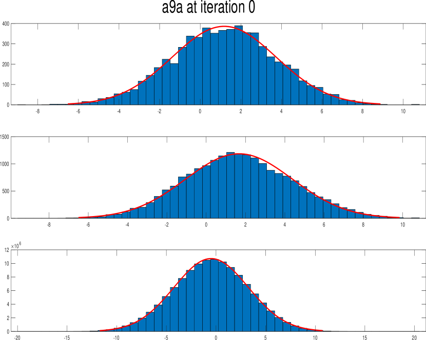
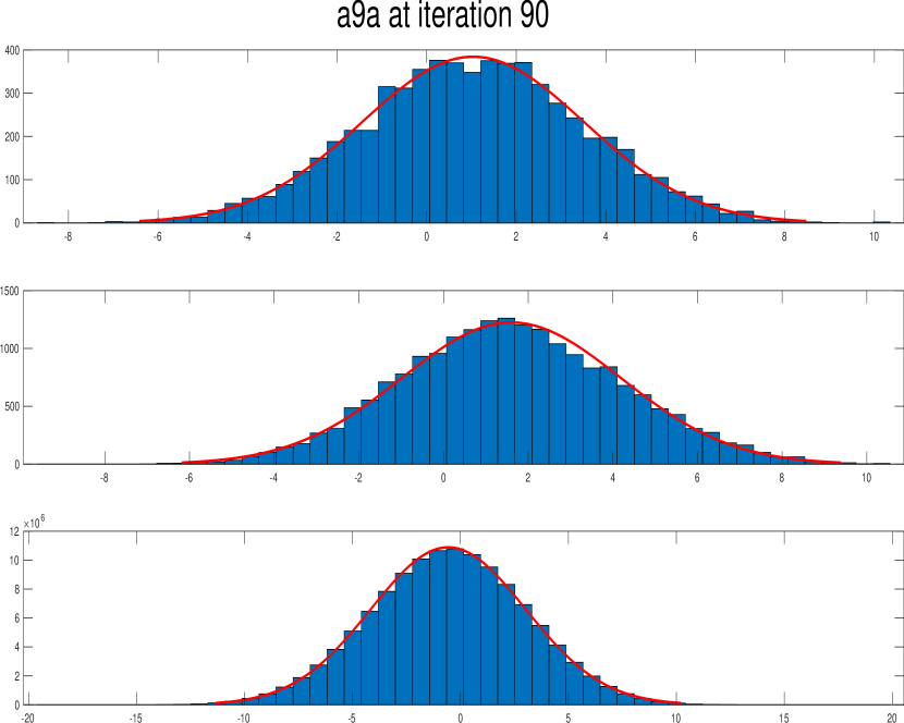
Figure 4.1: Nearly normal distribution for $w^{\top}X^{+}$, $w^{\top}X^{-}$ and $w^{\top}(X^{+}-X^{-})$ at different iterations during training.

We also present the plots for additional four datasets diabetes, poker, svm3 and segment in Figure 4.2. We observe that not in all cases random variables $w^{\top}X^{-}$, $w^{\top}X^{+}$, and $w^{\top}(X^{-}-X^{+})$ seem to have near normal distributions although it is more common for $w^{\top}(X^{-}-X^{+})$. Nevertheless our proposed functions $F_{n01}$ and $F_{nrank}$ still seem to provide useful approximations to empirical risk, as will be evident from the plots of these functions we present later in this section.

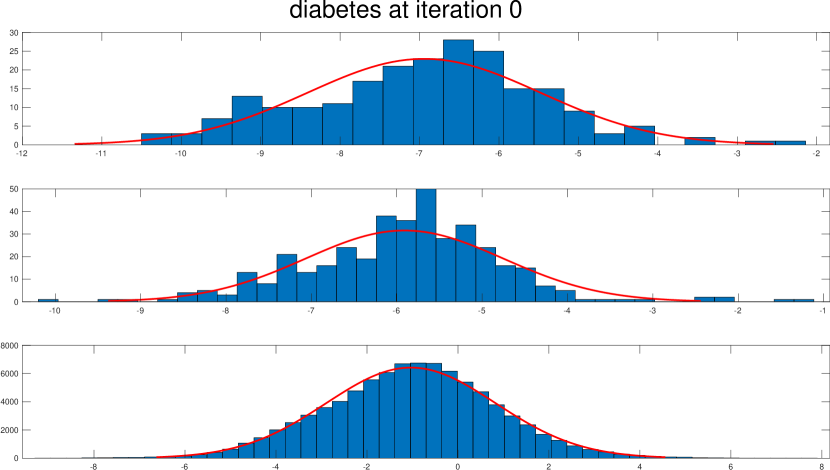
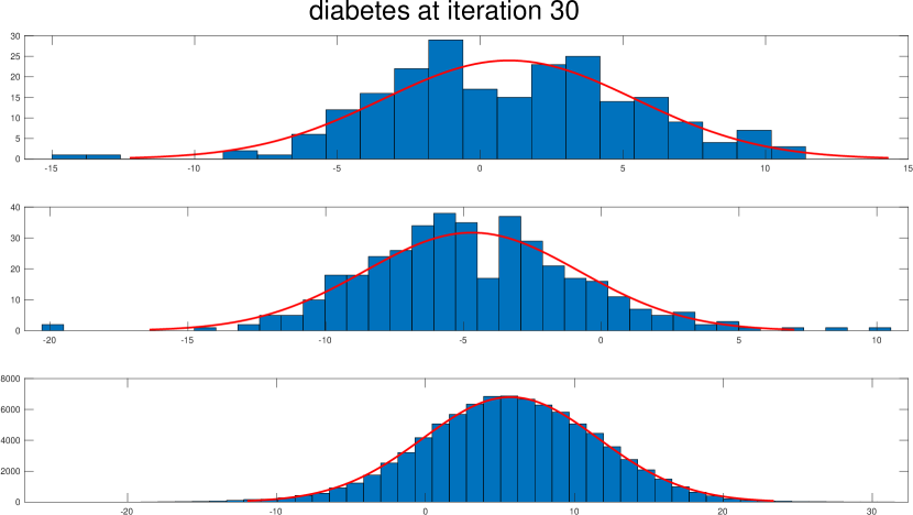
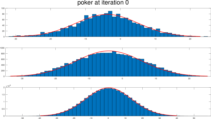
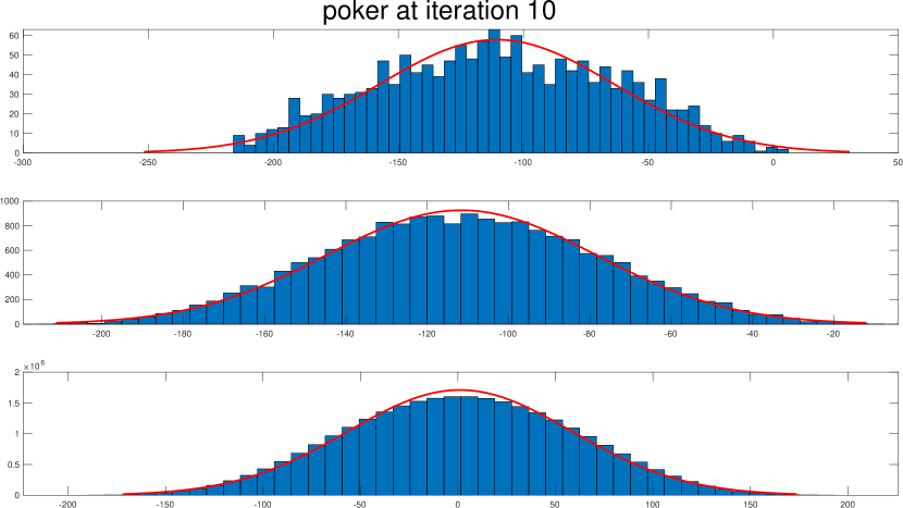
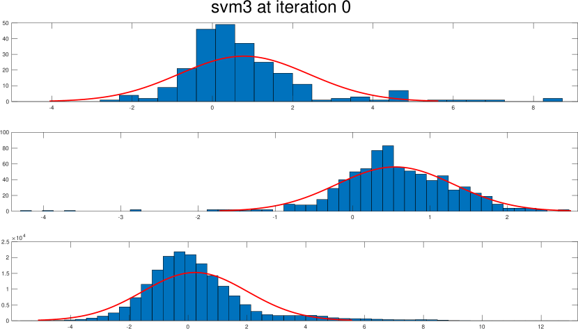
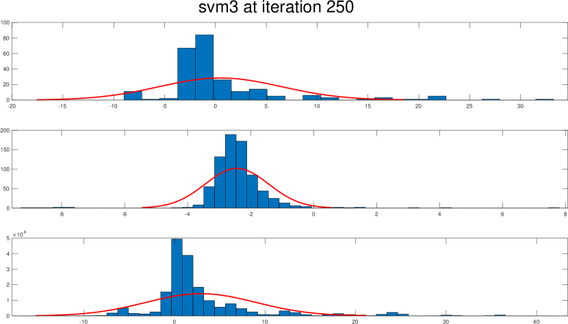
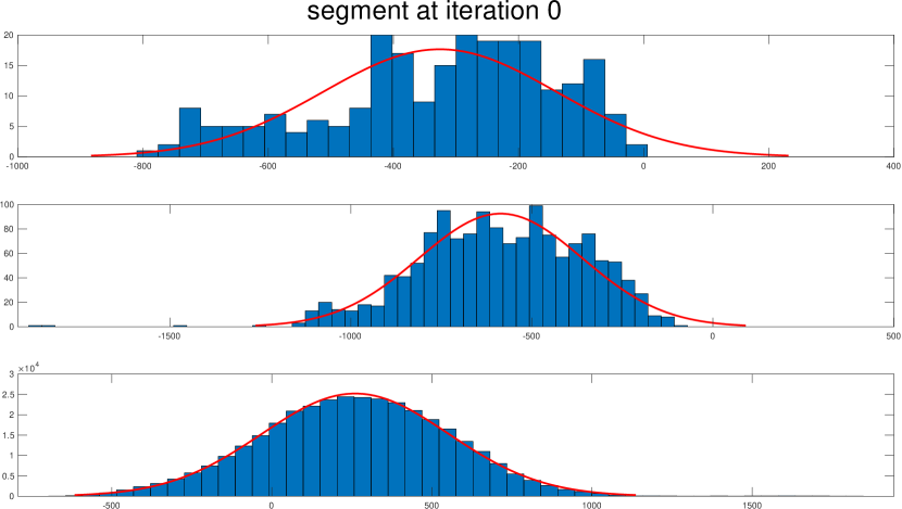
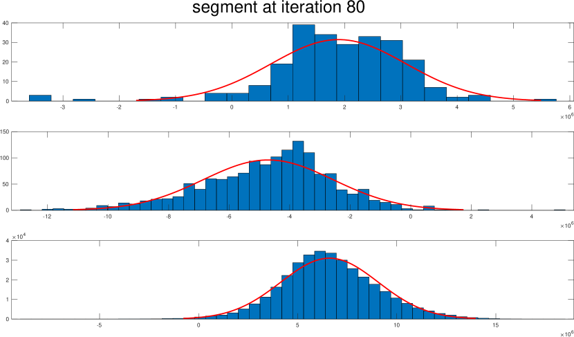
Figure 4.2: Distribution for $w^{\top}X^{+}$, $w^{\top}X^{-}$ and $w^{\top}(X^{+}-X^{-})$ at different iterations during training for diabetes.

We next demonstrate that minimizing our proposed models $F_{n01}$ and $F_{nrank}$ results in good classifiers and efficient training methods.

Method Based on the results of the previous section, we propose the following method of training a linear classifier for a given training set.

1. Using the positive and negative samples of the training set, compute the empirical estimates of $\mu^{+}$, $\mu^{-}$, as well as $\Sigma^{+}$, $\Sigma^{-}$ for the case of $F_{n01}$ and $\Sigma^{++}$, $\Sigma^{+-}$, $\Sigma^{+-}$, and $\Sigma^{--}$ for the case of $F_{nrank}$. Note that number of samples for positive and negative parts are not balanced and it is not clear how to get the empirical estimations of $\Sigma^{+-}$ and $\Sigma^{--}$. Theoretically, the random vectors with positive and negative labels should be uncorrelated and thus $\Sigma^{+-}$ and $\Sigma^{+-}$ are zero matrices. If we use some sampling methods to get the estimations for $\Sigma^{+-}$ and $\Sigma^{+-}$, the actual performance is worse than taking them as zero matrices.

2. By setting $P({Y}=1)=n_{+}/n$ and $P({Y}=-1)=n_{-}/n$, $F_{n01}(w)$ is defined as in (3.3) and $\nabla F_{n01}(w)$ is defined as in (3.5). Similarly, $F_{nrank}(w)$ is defined as in (3.8) and $\nabla F_{nrank}(w)$ is defined as in (3.10).

3. For minimizing the prediction error, apply L-BFGS method with Wolfe line-search until $w_{\epsilon}$ is reached such that $\|\nabla F^{\lambda}_{n01}(w)\|\leq\epsilon$, where $F^{\lambda}_{n01}(w)=F_{n01}(w)+\lambda(1-\|w\|^{2})^{2}$, for given a tolerance $\epsilon$. For ranking loss minimization apply the same to $F^{\lambda}_{nrank}(w)=F_{nrank}(w)+\lambda(1-\|w\|^{2})^{2}$. Return $w_{\epsilon}$ as the linear classifier.

Computational cost We compare the performance of the classifiers obtained by the proposed method to the state-of-the art linear classification methods. In particular, we compare optimizing $F^{\lambda}_{n01}$ vs. regularized logistic regression, and optimizing $F^{\lambda}_{nrank}$ vs. regularized pairwise hinge loss. The pairwise hinge loss is chosen as the most efficient surrogate for the ranking loss, because the cost of gradient computation is roughly ${\cal O}(n\log n)$, instead of ${\cal O}(n^{+}n^{-})$. For logistic regression we optimize function $\hat{F}^{\lambda}_{log}(w)=\hat{F}^{\lambda}_{log}(w)+\lambda\|w\|^{2}$ and for pairwise hinge loss we optimized $\hat{F}^{\lambda}_{hinge}(w)=\hat{F}^{\lambda}_{hinge}(w)+\lambda\|w\|^{2}$. We use L-BFGS method with Wolfe line-search for all four functions, $F^{\lambda}_{n01}$, $F^{\lambda}_{nrank}$ , $\hat{F}^{\lambda}_{log}(w)$ and $\hat{F}^{\lambda}_{hinge}(w)$. Even though $\hat{F}^{\lambda}_{hinge}(w)$ is not smooth, it is known that L-BFGS works very well for such functions [Lewis and Overton, 2013, Yu et al., 2010]. Note that each gradient computation for $\hat{F}^{\lambda}_{log}(w)$ and $\hat{F}^{\lambda}_{hinge}(w)$ require ${\cal O}(nd)$ and ${\cal O}(dn\log n)$ operations respectively (in the case of sparse data, the dependence on $d$ reduces according to sparsity). On the other hand applying the same method to $F^{\lambda}_{n01}$ and $F^{\lambda}_{nrank}$ requires only ${\cal O}(d^{2})$ operations, (and when the data is sparse, the dependence on $d$ reduces to as low as ${\cal O}(d)$, depending on the sparsity of the covariance matrices). The covariance matrix computation requires ${\cal O}(nd^{2})$ operations (${\cal O}(nd)$ in the sparse case), however, this computation is done once before the optimization algorithm. For the problems with large number of sparse features, such as rcv1 and realsim listed below, We can use the empirical covariance estimation in the form $\Sigma=\frac{1}{n-1}X^{T}X-\frac{n}{n-1}\bar{X}\bar{X}^{T}$ where $X$ is taken as the data matrix here and $\bar{X}$ is the mean vector of $X$. It is efficient in terms of both memory storage and computational cost since we don’t actually have to compute or store $\Sigma$ explicitly.

Alternative methods Note that function $F^{\lambda}_{n01}$ $F^{\lambda}_{nrank}$ have well defined Hessians as well, hence second order methods can be applied to minimize these functions. We have used preconditioned conjugate gradient method and other second order methods based on Hessian vector products, however, they did not outperform the L-BFGS in terms of time, while achieving similar accuracy.

Starting point $F^{\lambda}_{n01}(w)$ and $F^{\lambda}_{nrank}$ are nonconvex functions, thus the results of our optimization approach may depend on the starting point. In our experiments we used the following starting point

$$w_{0}=\frac{\bar{w}_{0}}{\|\bar{w}_{0}\|},\quad\text{where}\quad\bar{w}_{0}=\mu^{+}-\frac{{\mu^{-}}^{T}\mu^{+}}{\|\mu^{-}\|^{2}}\mu^{-}.$$

We have also tried random starting points, but the results were not better than using $w_{0}$ defined above. For logistic loss and hinge loss, we simply generate random starting points, since these functions are convex.

Details All experiments were run using Python3.5 on a Win10 with 3.60 GHz Intel Core i7 processor and 8GB of RAM. All functions were trained using L-BFGS with memory size set to $20$ and the Wolfe line-search parameters were set as $c1=0.0001,c2=0.9$. The maximum number of iterations was set to 500 and the first order optimal threshold was chosen as $10^{-4}$.

Artificial data For our first set of experiments, we have generated 9 different artificial Gaussian data sets of various dimensions using random first and second moments; they are summarized in Table 4.1. Moreover, for each set we generated some percentage of outliers by swapping labels of positive and negative examples in the training data. We set the regularization parameter to zero for the experiments with artificial data sets.

Table 4.1: Artificial data sets statistics. $d:$ number of features, $n:$ number of data points, $P^{+},P^{-}:$ prior probabilities, $out:$ percentage of outlier data points.

Name	$d$	${n}$	$P^{+}$	$P^{-}$	$out\%$
$data_{1}$	500	5000	0.05	0.95	0
$data_{2}$	500	5000	0.35	0.65	5
$data_{3}$	500	5000	0.5	0.5	10
$data_{4}$	1000	5000	0.15	0.85	0
$data_{5}$	1000	5000	0.4	0.6	5
$data_{6}$	1000	5000	0.5	0.5	10
$data_{7}$	2500	5000	0.1	0.9	0
$data_{8}$	2500	5000	0.35	0.65	5
$data_{9}$	2500	5000	0.5	0.5	10

The corresponding numerical results for $F_{n01}(w)$ are summarized in Table 4.2, where we used 80 percent of the data points as the training data and the rest as the test data. The reported average accuracy is based on 20 runs for each data set. When minimizing $F_{n01}(w)$, we used the exact moments from which the data set was generated, and also the approximate moments, empirically obtained from the training data. The bold numbers indicate the average testing accuracy attained by minimizing $F_{n01}(w)$ using approximate moments, when this accuracy is significantly better than that obtained by minimizing $F_{log}(w)$.

We see in Table 4.2 that, as expected, minimizing $F_{n01}(w)$ using the exact moments produces linear classifiers with superior performance overall, while minimizing $F_{n01}(w)$ using approximate moments outperforms minimizing $F_{log}(w)$, except for data8 and data9 where the number of data points is small compared to dimension and the moments estimates are not accurate. Note also that minimizing $F_{n01}(w)$ requires less time than minimizing $F_{log}(w)$.

Table 4.2: $F_{n01}(w)$ vs. $F_{log}(w)$ minimization on artificial data sets.

Data	$\boldsymbol{F_{n01}(w)}$ Minimization		$\boldsymbol{F_{n01}(w)}$ Minimization		$\boldsymbol{F_{log}(w)}$ Minimization
	Exact moments		Approximate moments
	Accuracy$\pm$ std	Time (s)	Accuracy $\pm$ std	Time (s)	Accuracy $\pm$ std	Time (s)
$data_{1}$	0.9965$\pm$0.0008	0.25	0.9907$\pm$0.0014	1.04	0.9897$\pm$0.0018	3.86
$data_{2}$	0.9905$\pm$0.0023	0.26	0.9806$\pm$0.0032	0.86	0.9557$\pm$0.0049	13.72
$data_{3}$	0.9884$\pm$0.0030	0.03	0.9745$\pm$0.0037	1.28	0.9537$\pm$0.0048	15.79
$data_{4}$	0.9935$\pm$0.0017	0.63	0.9791$\pm$0.0034	5.51	0.9782$\pm$0.0031	10.03
$data_{5}$	0.9899$\pm$0.0026	5.68	0.9716$\pm$0.0048	10.86	0.9424$\pm$0.0055	28.29
$data_{6}$	0.9904$\pm$0.0017	0.83	0.9670$\pm$0.0058	5.18	0.9291$\pm$0.0076	25.47
$data_{7}$	0.9945$\pm$0.0019	4.79	0.9786$\pm$0.0028	32.75	0.9697$\pm$0.0031	43.20
$data_{8}$	0.9901$\pm$0.0013	9.96	0.9290$\pm$0.0045	119.64	0.9263$\pm$0.0069	104.94
$data_{9}$	0.9899$\pm$0.0028	1.02	0.9249$\pm$0.0096	68.91	0.9264$\pm$0.0067	123.85

In Table 4.3 we compare the performance of linear classifiers obtained by optimizing $F_{nrank}(w)$ defined in (3.8) and the pairwise hinge loss, $\hat{F}(w)=F_{hinge}(w)$ as is defined in (2.8) on the artificial data described in Tables 4.1.

The results are summarized as in Table 4.2, except that we report the AUC value as the performance measure. As we can see in Table 4.3, the performance of the linear classifier obtained through minimizing $F_{nrank}(w)$ using approximate moments surpasses that of the classifier obtained via minimizing $\hat{F}_{hinge}(w)$, both in terms of the average AUC value as well as the required solution time.

Table 4.3: $F_{nrank}(w)$ vs. $F_{hinge}(w)$ minimization on artificial data sets.

Data	$\boldsymbol{F_{AUC}(w)}$ Minimization		$\boldsymbol{F_{AUC}(w)}$ Minimization		$\boldsymbol{F_{hinge}(w)}$ Minimization
	Exact moments		Approximate moments
	AUC$\pm$ std	Time (s)	AUC $\pm$ std	Time (s)	AUC $\pm$ std	Time (s)
$data_{1}$	0.9972$\pm$0.0014	0.01	0.9941$\pm$0.0027	0.23	0.9790$\pm$0.0089	5.39
$data_{2}$	0.9963$\pm$0.0016	0.01	0.9956$\pm$0.0018	0.22	0.9634$\pm$0.0056	159.23
$data_{3}$	0.9965$\pm$0.0015	0.01	0.9959$\pm$0.0018	0.24	0.9766$\pm$0.0041	317.44
$data_{4}$	0.9957$\pm$0.0018	0.02	0.9933$\pm$0.0022	0.83	0.9782$\pm$0.0054	23.36
$data_{5}$	0.9962$\pm$0.0011	0.02	0.9951$\pm$0.0013	0.80	$0.9589\pm$0.0068	110.26
$data_{6}$	0.9962$\pm$0.0013	0.02	0.9949$\pm$0.0015	0.82	0.9470$\pm$0.0086	275.06
$data_{7}$	0.9965$\pm$0.0021	0.08	0.9874$\pm$0.0034	4.61	0.9587$\pm$0.0092	28.31
$data_{8}$	0.9966$\pm$0.0008	0.07	0.9929$\pm$0.0017	4.54	0.9514$\pm$0.0051	104.16
$data_{9}$	0.9962$\pm$0.0014	0.08	0.9932$\pm$0.0020	4.54	0.9463$\pm$0.0085	157.62

Real data We now compare the performance of $F_{n01}$ vs. logistic regression and $F_{nrank}$ vs. pairwise hinge loss on 21 data sets downloaded from LIBSVM website and UCI machine learning repository, summarized in Table 4.4. The data sets from UCI machine learning repository with categorical features are transformed into grouped binary features. We have normalized the data sets so that each feature does not exceed $1$ in absolute value.

Table 4.4: Data sets statistics. $d:$ number of features, $n:$ number of data points, $P^{+},P^{-}:$ prior probabilities,
$AC:$ attribute characteristics.

Name	AC	$d$	${n}$	$P^{+}$	$P^{-}$
fourclass	real	2	862	0.35	0.65
svm1	real	4	3089	0.35	0.65
diabetes	real	8	768	0.35	0.65
vowel	int	10	528	0.09	0.91
magic04	real	10	19020	0.35	0.65
poker	int	11	25010	0.02	0.98
letter	int	16	20000	0.04	0.96
segment	real	19	210	0.14	0.86
svm3	real	22	1243	0.23	0.77
ijcnn1	real	22	35000	0.1	0.9
german	real	24	1000	0.3	0.7
landsat satellite	int	36	4435	0.09	0.91
sonar	real	60	208	0.5	0.5
a9a	binary	123	32561	0.24	0.76
w8a	binary	300	49749	0.02	0.98
mnist	real	782	100000	0.1	0.9
colon-cancer	real	2000	62	0.35	0.65
gisette	real	5000	6000	0.49	0.51
covtype	binary	54	581012	0.49	0.51
rcv1	real	47236	20242	0.52	0.48
real-sim	real	20958	72309	0.31	0.69

We used five-fold cross-validation using random data split and repeated each experiment four times, the results reported are averaged over 20 runs. The regularization parameter $\lambda$ for $F^{\lambda}_{n01}$ has been set to $0.001$ as this has been observed to be a good fixed value, while for $\hat{F}^{\lambda}_{log}$ it has been set to $1/n$, which is often suggested in the literature. Full tuning of $\lambda$ for both models can be performed, however, the effect of different $\lambda$ on minimization of $F^{\lambda}_{n01}$ is somewhat different from the usual regularization, since the function and the regularizer is not convex and local minima may be observed. On the other hand, tuning $\lambda$ for logistic regression is computationally costly.

In Table 4.5 we see the comparison of the average testing accuracy of the resulting linear classifier as well as the average number of iterations performed by the algorithms and the average CPU time. We can see that in almost all cases the testing accuracy achieved by both methods is very similar, with a few cases when one approach dominates the other. However, the solution time of our method is often much smaller, especially on large instances.

Table 4.5: Comparison of minimizing $F_{n01}(w)$ vs. $F_{log}(w)$.

	$\boldsymbol{F_{n01}}$				$\boldsymbol{F_{log}}$
Data	accuracy	num. iters	sol time	moment time	accuracy	num. iters	sol time
fourclass	0.7564$\pm$ 0.0323	10.35	0.01$\pm$ 0.00	0.00	0.7602$\pm$ 0.0293	7.45	0.01$\pm$ 0.00
svm1	0.9455$\pm$ 0.0092	23.75	0.03$\pm$ 0.00	0.00	0.9306$\pm$ 0.0131	16.00	0.02$\pm$ 0.00
diabetes	0.7667$\pm$ 0.0371	25.45	0.03$\pm$ 0.01	0.00	0.7680$\pm$ 0.0397	18.95	0.01$\pm$ 0.00
vowel	0.9619$\pm$ 0.0207	36.60	0.05$\pm$ 0.00	0.00	0.9652$\pm$ 0.0176	18.70	0.01$\pm$ 0.00
magic	0.7665$\pm$ 0.0091	43.05	0.06$\pm$ 0.00	0.00	0.7897$\pm$ 0.0087	25.55	0.04$\pm$ 0.01
poker	0.9795$\pm$ 0.0017	16.10	0.02$\pm$ 0.00	0.00	0.9795$\pm$ 0.0017	30.75	0.07$\pm$ 0.01
letter	0.9710$\pm$ 0.0030	85.65	0.13$\pm$ 0.01	0.00	0.9824$\pm$ 0.0019	67.10	0.12$\pm$ 0.02
segment	0.9845$\pm$ 0.0292	401.25	0.65$\pm$ 0.22	0.00	0.9978$\pm$ 0.0022	97.85	0.11$\pm$ 0.01
svm3	0.8208$\pm$ 0.0245	214.25	0.33$\pm$ 0.04	0.00	0.7929$\pm$ 0.0209	18.90	0.02$\pm$ 0.00
ijcnn1	0.9054$\pm$ 0.0026	41.9	0.07$\pm$ 0.01	0.00	0.9142$\pm$ 0.0025	32.00	0.10$\pm$ 0.02
german	0.7553$\pm$ 0.0252	35.30	0.05$\pm$ 0.00	0.00	0.7648$\pm$ 0.0320	25.60	0.02$\pm$ 0.00
satimage	0.9064$\pm$ 0.0064	13.00	0.02$\pm$ 0.00	0.00	0.9068$\pm$ 0.0060	490.75	0.70$\pm$ 0.03
sonar	0.7573$\pm$ 0.0610	500.00	0.66$\pm$ 0.01	0.00	0.7549$\pm$ 0.0761	14.90	0.01$\pm$ 0.00
a9a	0.8376$\pm$ 0.0043	130.10	0.35$\pm$ 0.04	0.02	0.8472$\pm$ 0.0041	75.85	1.27$\pm$ 0.09
w8a	0.9807$\pm$ 0.0013	273.95	2.00$\pm$ 0.12	0.07	0.9842$\pm$ 0.0012	24.90	1.60$\pm$ 0.16
mnist	0.9819$\pm$ 0.0008	500.00	16.49$\pm$ 0.21	0.54	0.9877$\pm$ 0.0005	112.55	36.88$\pm$ 2.21
colon	0.7833$\pm$ 0.1191	17.50	0.48$\pm$ 0.06	0.04	0.7167$\pm$ 0.1221	54.15	0.11$\pm$ 0.01
gisette	0.9753$\pm$ 0.0035	83.30	14.60$\pm$ 2.38	1.06	0.9714 $\pm$ 0.0043	156.10	21.64$\pm$ 1.79
covtype	0.5502$\pm$ 0.0134	500.00	7.93$\pm$ 0.13	0.11	0.7562$\pm$0.0010	97.50	15.87$\pm$2.35
rcv1	0.9632$\pm$ 0.0026	73.35	26.54$\pm$ 2.32	1.37	0.9595$\pm$ 0.0024	15.30	56.37$\pm$ 1.95
realsim	0.9547$\pm$ 0.0018	500.00	263.84$\pm$10.19	2.67	0.9676$\pm$0.0014	16.65	1367.80$\pm$62.33

Table 4.6: Comparison of minimizing $F_{nrank}(w)$ vs. $F_{hinge}(w)$.

	$\boldsymbol{F_{nrank}}$				$\boldsymbol{F_{hinge}}$
Data	accuracy	num. iters	sol time	moment time	accuracy	num. iters	sol time
fourclass	0.8362$\pm$ 0.0312	7.00	0.01$\pm$ 0.00	0.00	0.8361$\pm$ 0.0312	11.95	0.15$\pm$ 0.01
svm1	0.9717$\pm$ 0.0065	13.20	0.01$\pm$ 0.00	0.00	0.9841$\pm$ 0.0041	11.95	0.53$\pm$ 0.04
diabetes	0.8311$\pm$ 0.0312	14.65	0.01$\pm$ 0.00	0.00	0.8308$\pm$ 0.0329	20.80	0.29$\pm$ 0.25
shuttle	0.9840$\pm$ 0.0016	63.90	0.07$\pm$ 0.01	0.00	0.9892$\pm$ 0.0015	12.85	8.66$\pm$ 0.48
vowel	0.9585$\pm$ 0.0333	19.30	0.02$\pm$ 0.00	0.00	0.9737$\pm$ 0.0202	36.35	0.34$\pm$0.17
magic	0.8382$\pm$ 0.0071	22.30	0.02$\pm$ 0.00	0.00	0.8428$\pm$ 0.0070	20.25	5.74$\pm$ 0.49
poker	0.5053$\pm$ 0.0224	15.75	0.02$\pm$ 0.00	0.00	0.5070$\pm$ 0.0223	28.80	11.26$\pm$ 2.55
letter	0.9830$\pm$ 0.0029	23.45	0.02$\pm$ 0.00	0.00	0.9884$\pm$ 0.0022	31.25	9.00$\pm$ 1.36
segment	0.9947$\pm$ 0.0055	261.30	0.27$\pm$ 0.15	0.00	0.9999$\pm$ 0.0001	37.60	1.28$\pm$0.22
svm3	0.7996$\pm$ 0.0421	115.95	0.67$\pm$ 0.08	0.00	0.7731$\pm$ 0.0457	25.55	0.48$\pm$ 0.08
ijcnn1	0.9269$\pm$ 0.0036	31.00	0.03$\pm$ 0.00	0.00	0.9291$\pm$ 0.0037	35.55	19.48$\pm$ 0.99
german	0.7938$\pm$ 0.0292	26.90	0.03$\pm$ 0.00	0.00	0.7929$\pm$ 0.0292	35.60	0.56$\pm$ 0.08
satimage	0.7561$\pm$ 0.0163	80.00	0.09$\pm$ 0.02	0.00	0.7665$\pm$ 0.0193	78.00	5.33$\pm$ 1.36
sonar	0.8150$\pm$ 0.0672	500.00	0.51$\pm$ 0.01	0.00	0.8470$\pm$ 0.0559	113.90	0.77$\pm$ 1.17
a9a	0.9002$\pm$ 0.0040	205.90	0.24$\pm$ 0.04	0.02	0.9033$\pm$ 0.0037	81.15	48.04$\pm$2.50
w8a	0.9631$\pm$ 0.0058	422.75	0.58 $\pm$ 0.05	0.07	0.9659$\pm$ 0.0049	400.05	606.08$\pm$ 137.09
mnist	0.9942$\pm$ 0.0009	500.00	0.88$\pm$ 0.07	0.55	0.9953 $\pm$ 0.0007	70.80	516.67$\pm$ 21.13
colon	0.8715$\pm$ 0.0933	13.40	0.16$\pm$ 0.01	0.04	0.8774$\pm$ 0.0998	78.35	0.58$\pm$ 0.20
gisette	0.9962$\pm$ 0.0012	20.60	1.61$\pm$ 0.08	1.05	0.9943$\pm$ 0.0013	73.95	107.49$\pm$ 23.64
covtype	0.8243$\pm$ 0.0001	240.20	0.24$\pm$ 0.02	0.11	0.8272$\pm$ 0.0009	192.65	1872.67$\pm$ 104.84
rcv1	0.9934$\pm$ 0.0008	15.90	5.38$\pm$ 0.32	1.42	0.9941$\pm$0.0008	23.50	3712.87$\pm$ 229.71
realsim	0.9916$\pm$ 0.006	46.20	20.16$\pm$ 1.22	2.82

In Table 4.6 we compare the average testing AUC of two linear classifiers as well as the average number of iterations performed by the algorithms and the average CPU time. For these experiments we set $\lambda$ to $0.001$ for $F^{\lambda}_{nrank}$, but for $\hat{F}^{\lambda}_{hinge}$ we set it to $1/\sqrt{n^{+}n^{-}}$, to mimic the choice of the regularization term in the case of logistic regression. We can see that testing AUC is almost the same for both methods while the solution time of our proposed model is significantly smaller than that for $\hat{F}^{\lambda}_{hinge}$. In fact, we could not obtain solution when minimizing real_sim within 24 hours. This difference is due to the fact that the complexity of each iteration of pairwise hinge loss optimization is superlinear in terms of $n$, while our function $F^{\lambda}_{nrank}$ has no dependence on $n$ at all.

Numerical Comparison vs. LDA and ADAM To support our observation further, we present comparison of the linear classifiers obtained by our proposed method to those obtained by Linear Discriminant Analysis (LDA) which is a well-known method to produce linear classifiers under the Gaussian assumption. We observe that the accuracy obtained by LDA classifiers is comparable with the other two but is significantly worse for data sets like svm1 and gisette. In the attempt to reduce the dependence of the complexity of optimizing $\hat{F}^{\lambda}_{log}(w)$ and $\hat{F}^{\lambda}_{hinge}(w)$ on $n$, we also applied popular version of stochastic gradient descent, Adam [Kingma and Ba, 2015] to the regularized logistic regression $\hat{F}^{\lambda}_{log}(w)$. Note that there is no reason to apply stochastic gradient descent methods to $F_{n01}(w)$, since the dependence on $n$ is removed from per-iteration complexity.

The parameters for ADAM we chosen as recommended in [Kingma and Ba, 2015], i.e. fixed step size $\alpha=0.001$, $\beta_{1}=0.9$, $\beta_{2}=0.999$ and $\epsilon=10^{-8}$. However, the results were sensitive to the choice of batch size and number of epochs. In our experiment, after some hand tuning, we chose the number of epochs to be $500$, the same as the maximum number of iterations for deterministic method and batch size is chosen to be $200$ for most data sets. The results are summarized in Table 4.7. For colon, batch size is chosen to be $10$ and for vowel, sonar, batch size is chosen to be $20$, since the numbers of samples for these data sets are small. In poker, letter, segment, ijcnn1, w8a, ADAM achieved comparable performance as $F_{log}$, but in other cases, it did not achieve the same accuracy as L-BFGS. LDA results have been obtained by employing the scikit-learn Python package and are clearly inferior to minimizing either $F_{n01}(w)$ or $F_{log}(w)$. Both LDA and ADAM are too slow for large scale data sets such as rcv1 and realsim because of large dimension $d$, hence we we did not report results on these two sets.

Table 4.7: Comparison of L-BFGS applied to $F_{n01}(w)$ and $F_{log}(w)$ vs. ADAM applied to $F_{log}(w)$ and LDA.

Data	$\boldsymbol{F_{n01}(w)}$ Minimization	$\boldsymbol{F_{log}(w)}$ Minimization	LDA	ADAM
	Accuracy$\pm$ std	Accuracy $\pm$ std	Accuracy $\pm$ std	Accuracy $\pm$ std
fourclass	0.7564$\pm$ 0.0323	0.7602$\pm$ 0.0293	0.7572$\pm$0.0314	0.7378$\pm$0.0444
svm1	0.9455$\pm$ 0.0092	0.9306$\pm$ 0.0131	0.8972$\pm$0.0159	0.8417$\pm$0.0153
diabetes	0.7667$\pm$ 0.0371	0.7680$\pm$ 0.0397	0.7703$\pm$0.0366	0.7333$\pm$0.3860
vowel	0.9619$\pm$ 0.0207	0.9652$\pm$ 0.0176	0.9600$\pm$0.0224	0.9276$\pm$0.0238
magic	0.7665$\pm$ 0.0091	0.7897$\pm$ 0.0087	0.7841$\pm$0.0093	0.6590$\pm$0.0087
poker	0.9795$\pm$ 0.0017	0.9795$\pm$ 0.0017	0.9795$\pm$0.0017	0.9795$\pm$0.0017
letter	0.9710$\pm$ 0.0030	0.9824$\pm$ 0.0019	0.9711$\pm$0.0029	0.9709$\pm$0.0034
segment	0.9845$\pm$ 0.0292	0.9978$\pm$ 0.0022	0.9617$\pm$0.0331	0.9968$\pm$0.0032
svm3	0.8208$\pm$ 0.0245	0.7929$\pm$ 0.0209	0.8238$\pm$0.0259	0.7619$\pm$0.0192
ijcnn1	0.9054$\pm$ 0.0026	0.9142$\pm$ 0.0025	0.9081$\pm$0.0029	0.9024$\pm$0.0023
german	0.7553$\pm$ 0.0252	0.7648$\pm$ 0.0320	0.7675$\pm$0.0275	0.7355$\pm$ 0.0308
satimage	0.9064$\pm$ 0.0064	0.9068$\pm$ 0.0060	0.9061$\pm$0.0065	0.8761$\pm$0.0660
sonar	0.7573$\pm$ 0.0610	0.7549$\pm$ 0.0761	0.7622$\pm$0.0499	0.6768$\pm$0.0703
a9a	0.8376$\pm$ 0.0043	0.8472$\pm$ 0.0041	0.8452$\pm$0.0038	0.8066$\pm$0.0061
w8a	0.9807$\pm$ 0.0013	0.9842$\pm$ 0.0012	0.9839$\pm$0.0012	0.9703$\pm$0.0018
mnist	0.9819$\pm$ 0.0008	0.9877$\pm$ 0.0005	0.9778$\pm$0.0013	0.9722$\pm$0.0032
colon	0.7833$\pm$ 0.1191	0.7167$\pm$ 0.1221	0.8875$\pm$0.0985	0.7375$\pm$0.1332
gisette	0.9753$\pm$ 0.0035	0.9714 $\pm$ 0.0043	0.5875$\pm$0.0207	0.9338$\pm$ 0.0257
covtype	0.5502$\pm$ 0.0134	0.7562$\pm$0.0010	0.7553$\pm$0.0009	0.6304$\pm$0.0142

Accuracy of the new approximations We further illustrate the comparison of $F_{n01}$ and $\hat{F}_{log}$ by plotting these functions next to the function they are meant to approximate, which is the empirical training error $\hat{F}_{01}$. In Figure 4.3 we show several examples of such comparisons. We have selected a segment of different $w$’s from the starting point to the stopping point of the algorithm. We have generated $100$ equally spaced points along this path. Note that the start and the end are different for $F_{n01}$ and logistic regression, however, what we are trying to illustrate here is the quality of approximation these functions provide with respect to the true empirical error in the area of interest to the optimization algorithm. For each example, on the left side we plot $F_{n01}(w)$ in red and the empirical error in blue. On the right side we plot logistic regression in red and empirical error in blue, however, due to different scaling on the functions we had to separate their plots. We see that $F_{n01}$ overall provides a better approximation of the empirical error than logistic regression. In all cases aside from svm3 $F_{n01}$ behaves as a smoothed version of the empirical error. Logistic regression, on the other hand does not seem to approximate empirical error function at all in many cases, it only successfully predicts the area where the minimizers of $\hat{F}_{01}$ lie. Moreover, in the case of colon, which is the data set with only 62 data points, the accuracy achieved from $F_{n01}$ much better than that from logistic regression and we see that $F_{n01}$ is a very close approximation of $\hat{F}_{01}$. In Figure 4.4 we illustrate how $F_{nrank}$ and pairwise hinge loss approximate the empirical ranking loss function $\hat{F}_{rank}$. We observe that again $F_{nrank}$ provides good approximations to $\hat{F}_{rank}$ while $\hat{F}_{hinge}$ is only consistently good at approximating the minimizers.

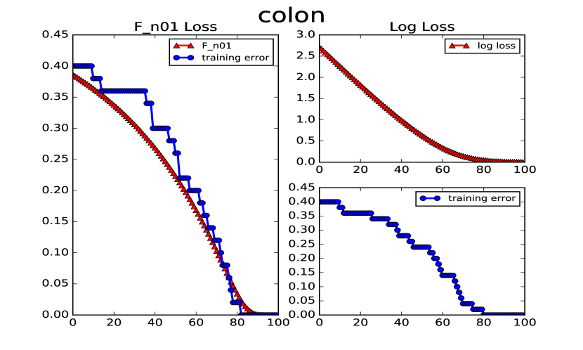
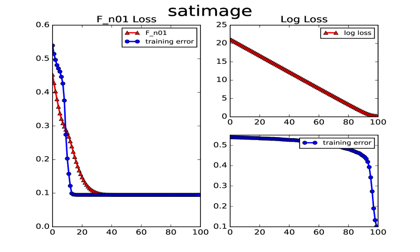
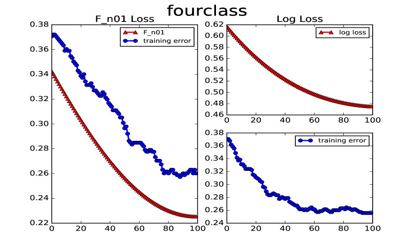
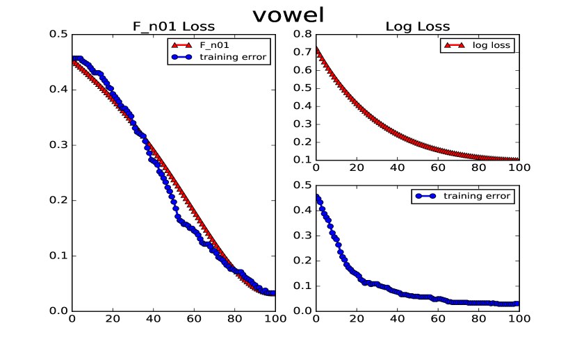
Figure 4.3: Approximating empirical loss by $F_{n01}$ and $\hat{F}_{log}$.

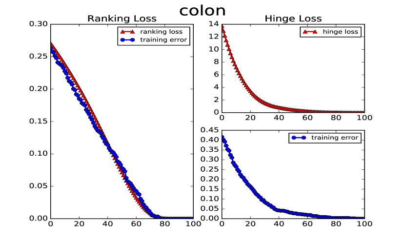
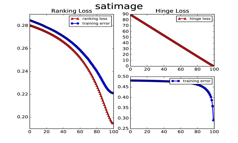
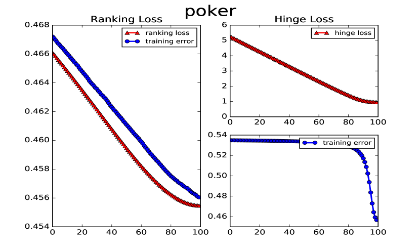
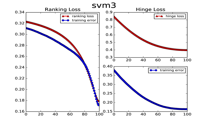
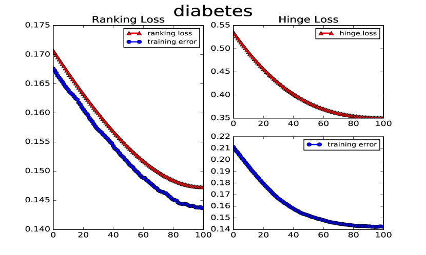
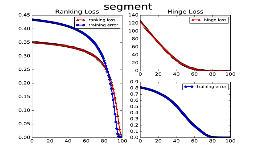
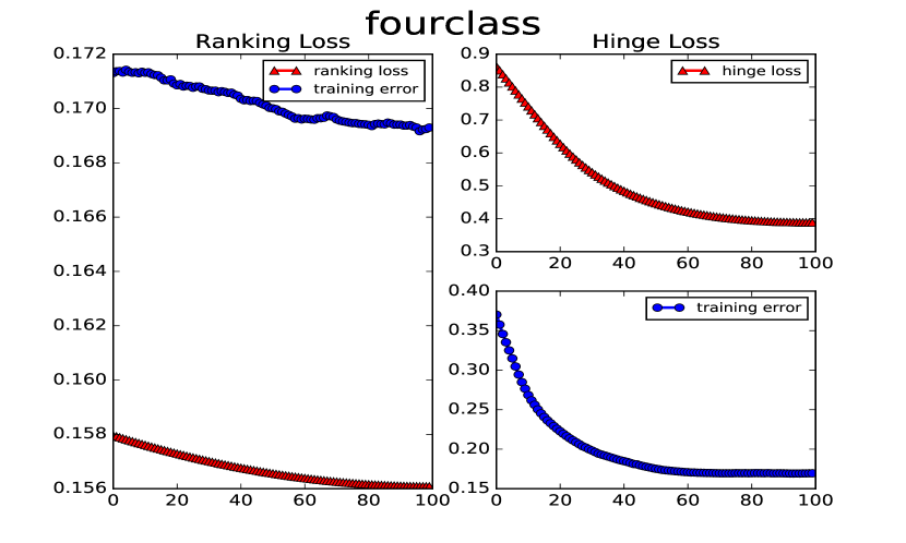
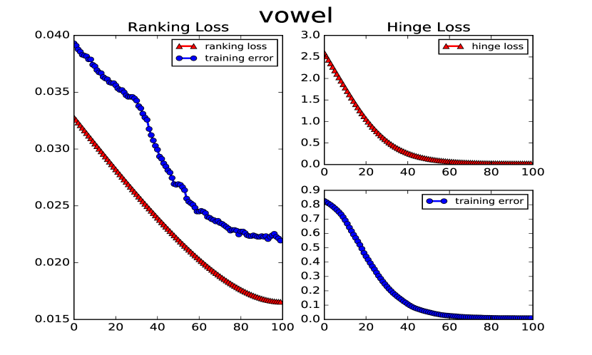
Figure 4.4: Approximating empirical ranking loss by $F_{nrank}$ and $\hat{F}_{hinge}$.

5 Conclusion

In this paper, we propose novel smooth approximation functions for the training error and ranking loss of linear predictors in binary classification, whose derivatives are expressed using the first and second moments of the related data distribution. We give theoretical motivation for why and when these functions may provide good approximation. We then propose to applying an optimization algorithm to these functions to obtain linear classifiers with the test accuracy and AUC comparable with those achieved by state-of-the-art methods. The main advantage of the proposed approximations is that their evaluation and that of their derivatives is independent of the size of the data sets, and hence optimization algorithms applied to them can be very efficient.

References

- [Billingsley, 1995] Billingsley, P. (1995). Probability and Measure. A Wiley-Interscience Publication.
- [Cheng et al., 2018] Cheng, F., Zhang, X., Zhang, C., Qiu, J., and Zhang, L. (2018). An adaptive mini-batch stochastic gradient method for auc maximization. Neurocomputing, 318:137–150.
- [Fisher and Sen, 1994] Fisher, N. I. and Sen, P. K. (1994). The central limit theorem for dependent random variables. in The Collected Works of Wassily Hoeffding, New York:Springer-Verlag, pages 205–213.
- [Hanley and McNeil, 1982] Hanley, J. A. and McNeil, B. J. (1982). The meaning and use of the area under a receiver operating characteristic (ROC) curve. Radiology.
- [Izenman, 2013] Izenman, A. J. (2013). Modern Multivariate Statistical Techniques. Springer Texts in Statistics.
- [Kingma and Ba, 2015] Kingma, D. P. and Ba, J. L. (2015). Adam: A method for stochastic optimization. ICLR, 2015.
- [Lewis and Overton, 2013] Lewis, A. S. and Overton, M. L. (2013). Nonsmooth optimization via quasi-newton methods. Mathematical Programming, 141:135–163.
- [Nocedal and Wright, 2006] Nocedal, J. and Wright, S. (2006). Numerical Optimization. Springer Series in Operations Research. Springer, New York, NY, USA, 2nd edition.
- [Rudin and Schapire, 2009] Rudin, C. and Schapire, R. E. (2009). Margin-based ranking and an equivalence between adaboost and rankboost. Journal of Machine Learning Research, 10:2193–2232.
- [Steck, 2007] Steck, H. (2007). Hinge rank loss and the area under the ROC curve. In ECML, Lecture Notes in Computer Science, pages 347–358.
- [Tong, 1990] Tong, Y. (1990). The multivariate normal distribution. Springer Series in Statistics.
- [Yan et al., 2003] Yan, L., Dodier, R., Mozer, M., and Wolniewicz, R. (2003). Optimizing classifier performance via approximation to the wilcoxon-mann-witney statistic. Proceedings of the Twentieth Intl. Conf. on Machine Learning, AAAI Press, Menlo Park, CA, pages 848–855.
- [Yu et al., 2010] Yu, J., Vishwanathan, S. N., Günter, S., and Schraudolph, N. N. (2010). A quasi-newton approach to nonsmooth convex optimization problems in machine learning. Journal of Machine Learning Research, 11:1–57.