Observations of the Ultraviolet-Bright Star Barnard 29 in the Globular Cluster M13 (NGC 6205)

Abstract

We have analyzed FUSE, COS, GHRS, and Keck HIRES spectra of the UV-bright star Barnard 29 in M13 (NGC 6205). By comparing the photospheric abundances derived from multiple ionization states of C, N, O, Si, and S, we infer an effective temperature $T_{\rm eff}$ = $21,400\pm 400$ K. Balmer-line fits yield a surface gravity $\log g$ = $3.10\pm 0.03$. We derive photospheric abundances of He, C, N, O, Mg, Al, Si, P, S, Cl, Ar, Ti, Cr, Fe, Ni, and Ge. Barnard 29 exhibits an abundance pattern typical of the first-generation (FG) stars in M13, enhanced in oxygen and depleted in aluminum. An underabundance of C and an overabundance of N suggest that the star experienced nonconvective mixing on the RGB. We see no evidence of significant chemical evolution since the star left the RGB; in particular, it did not undergo third dredge-up. Previous workers found that the star’s FUV spectra yield an iron abundance about 0.5 dex lower than its optical spectrum, but the iron abundances derived from all of our spectra are consistent with the cluster value. We attribute this difference to our use of model atmospheres without microturbulence, which is ruled out by careful fits to optical absorption features. We derive a mass $M_{*}/M_{\sun}=0.45-0.55$ and luminosity $\log L_{*}/L_{\sun}=3.26-3.35$. Comparison with stellar-evolution models suggests that Barnard 29 evolved from a ZAHB star of mass $M_{*}/M_{\sun}$ between 0.50 and 0.55, near the boundary between the extreme and blue horizontal branches.

1 Introduction

The bright, blue star Barnard 29 in Messier 13 (NGC 6205) has intrigued astronomers for more than a century. In a series of papers, Barnard (1900, 1909, 1914) pointed out that some of the cluster’s stars “shine with a much bluer light than the great majority” and cited Barnard 29 as the “most striking example” of this group. Smith (2005) reviews the early research into these hot, luminous objects, which are now referred to as UV-bright stars. Some are post-AGB stars, evolving from the asymptotic giant branch (AGB) to the white-dwarf cooling curve at high luminosity; others are AGB-manqué stars, evolving directly from the extreme horizontal branch (EHB) at lower luminosity. Modern spectroscopic studies of Barnard 29 include those of Conlon et al. (1994), Dixon & Hurwitz (1998), Moehler et al. (1998), and Thompson et al. (2007). They established the star as a post-AGB object with $T_{\rm eff}$ = $20,000\pm 1000$ K, $\log g$ = $2.95\pm 0.1$, and $\log N({\rm He})/N({\rm H})$ = $-1.06\pm 0.20$ and determined its photospheric abundances of C, N, O, Mg, Al, Si, S, and Fe. Its radial velocity ($V_{\rm LSR}=-228$ km s^-1; Thompson et al. 2007) is consistent with the cluster mean ($V_{\rm LSR}=-228.0$ km s^-1; Harris 1996, 2010).

Despite over a century of study, important questions about Barnard 29 remain unanswered. In particular, the iron abundance derived from the star’s far-ultraviolet (FUV) spectrum is roughly 0.5 dex lower than that derived from optical data, which is consistent with the cluster mean (Thompson et al., 2007). Another question concerns the extent to which the star’s photospheric abundances have been altered by evolutionary processes, particularly nucleosynthesis on the AGB. The availability of high-resolution, high signal-to-noise FUV and optical spectra allow us to confirm the star’s iron abundance and determine the abundances of many additional species. We employ archival spectra from the Far Ultraviolet Spectroscopic Explorer (FUSE), the Cosmic Origins Spectrograph (COS) and Goddard High Resolution Spectrometer (GHRS) aboard the Hubble Space Telescope, and the Keck High Resolution Echelle Spectrometer (HIRES). A summary of these data is presented in Table 1. A link to the FUSE and HST data is provided here: http://doi.org/10.17909/T9ZH6R (catalog 10.17909/T9ZH6R).

In Section 2, we describe these observations and our reduction of the data. We present our determination of the star’s effective temperature and chemical abundances in Section 3.1 and its surface gravity and helium abundance in Section 3.2. We describe our model atmospheres in Section 3.3 and our fitting procedure in Section 3.4. We discuss challenges presented by specific stellar features in Section 4.1 and examine the implications of our photospheric abundances in Section 4.2. We estimate the star’s mass, radius, and luminosity in Section 4.3 and discuss its evolutionary status in Section 4.4. Finally, we summarize our conclusions in Section 5.

Table 1: Summary of FUSE, COS, GHRS, and Keck Observations

Instrument	Grating	Wavelength	$R\equiv\lambda/\Delta\lambda$	Exp. Time	Obs. Date	Data ID	P.I.
		(Å)		(s)
FUSE	$\cdots$	0905–1187	20,000	15,572	2000 Aug 3	P1015201	Sembach
COS	G130M	1130–1430	10,000	00.550	2010 Jul 14	LB2401020	Green
COS	G160M	1410–1780	18,000	00.625	2010 Jul 14	LB2401010	Green
GHRS	G200M	1865–1905	20,000	0.4570	1996 Nov 30	Z3EC0204T	Napiwotzki
HIRES	$\cdots$	4300–6700	47,800	0.1500	1996 Jun 5	HI.19960605.40896	Reid

2 Observations and Data Reduction

2.1 FUSE Spectroscopy

The Far Ultraviolet Spectroscopic Explorer (FUSE) provides medium-resolution spectroscopy from 1187 Å to the Lyman limit (Moos et al., 2000; Sahnow et al., 2000). Barnard 29 was observed through the FUSE $30\arcsec\times 30\arcsec$ aperture. The data were reduced using v3.2.1 of CalFUSE, the standard data-reduction pipeline software (Dixon et al., 2007). CalFUSE corrects for a variety of instrumental effects, extracts spectra from each of the four FUSE channels, and performs wavelength and flux calibration. The extracted spectra are binned by 0.013 Å, which corresponds to about 2 detector pixels, or one-fourth of a point-source resolution element. The spectra from each exposure are aligned by cross-correlating on the positions of stellar absorption features and combined into a single spectrum for each channel. The signal-to-noise ratio (S/N) per resolution element is about 20 at wavelengths shorter than 1000 Å and about 30 at longer wavelengths. The spectrum shows absorption from C, N, O, Al, Si, P, S, Cl, Ar, Cr, Fe, Ni, and Ge.

Lehner et al. (2004) used this spectrum in a survey designed to study the rate of radiative cooling in the diffuse interstellar medium (ISM). They combined column-density measurements of C II*, S II, P II, and Fe II with H I 21 cm emission measurements to derive the cooling rates and analyze the ionization structure, depletion, and metallicity of low-, intermediate-, and high-velocity clouds (LVCs, IVCs, and HVCs) along a number of high-latitude sight lines.

2.2 COS Spectroscopy

The Cosmic Origins Spectrograph (COS) enables high-sensitivity, medium- and low-resolution spectroscopy in the 1150–3200 Å wavelength range (Green et al., 2012). Barnard 29 was observed with COS using both the G130M and G160M gratings. The fully-reduced spectra, processed with CALCOS version 3.2.1 (Fox, 2015), were retrieved from the Mikulski Archive for Space Telescopes (MAST). The S/N varies between 45 and 65 per 7-pixel resolution element in the G130M spectrum. In the G160M spectrum, the S/N falls monotonically from $\sim 60$ at 1430 Å to $\sim 20$ at 1770 Å. The spectrum shows absorption from He, C, N, O, Mg, Al, Si, S, Ti, Cr, Fe, Ni, and Ge.

The G160M exposures were obtained first, in time-tag mode, followed by a pair of G130M exposures. Because the star is bright at short wavelengths, the G130M exposures were obtained in ACCUM mode, which can accommodate higher count rates. The use of ACCUM mode had two effects on the data: First, the resolution of the G130M spectrum is significantly lower than the nominal value for this grating ($R\sim 18,000$); modeling the line-spread function with a Gaussian yields FWHM = 0.13 Å ($R\sim 10,000$). The motion of the COS Optics Select Mechanism 1 (OSM1), which is used to switch between gratings, is not perfectly controlled and can continue throughout an exposure, which in turn moves the spectrum across the detector in an effect known as OSM drift (White et al., 2016). Time-tag data can be corrected for OSM drift (CALCOS does this automatically), but ACCUM data cannot, resulting in a lower spectral resolution for the G130M spectrum.

The second effect is an error in the wavelength solution for the first G130M exposure. The spectra produced by the two exposures are nearly identical on detector segment B (1130 – 1280 Å), but are offset by about 6 pixels at the short-wavelength end of segment A (1290 – 1430 Å) and by more than 40 pixels – nearly 0.5 Å – at the long-wavelength end. When taking data in ACCUM mode, COS follows each external exposure with a short exposure of a wavelength-calibration lamp; perhaps the first cal-lamp spectrum was distorted by OSM drift. We correct for the wavelength error by determining the shift between the two spectra in 10 Å bins across segment A, fitting a linear function to the measured offsets, and rescaling the wavelength array of the first exposure. Rather than combining the two spectra, we feed both of them to our fitting routines and fit them simultaneously.

Welsh et al. (2011) used the COS and FUSE spectra to study the ISM toward M13. They detected absorption due to C I, C II, C II*, C IV, N I, N II, N V, O I, Al II, Si II, Si IV, S II, and Fe II at $V_{\rm LSR}\sim-60$ km s^-1, associated with a well-known IVC, and absorption due to C II, C III, C IV, N II, Si II, and Si IV at $V_{\rm LSR}=-121\pm 3$ km s^-1, which they identified as a previously unknown highly-ionized, multi-phase HVC.

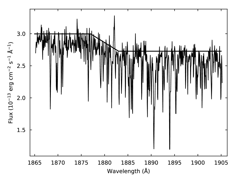
Figure 1: GHRS spectrum of Barnard 29, overplotted with our estimate of the continuum. For this figure, the data are binned by three pixels. Wavelengths are in the observed frame.

2.3 GHRS Spectroscopy

The Goddard High-Resolution Spectrograph (GHRS) was one of the four original axial instruments aboard the Hubble Space Telescope (Heap et al., 1995). Barnard 29 was observed through the Large Science Aperture (LSA) with the G200M grating. The fully-reduced spectrum, a product of the final re-calibration of the GHRS data set, was retrieved from MAST. The spectrum, reproduced in Fig. 1, spans the wavelength range 1865–1905 Å, a bandpass chosen to enable a measurement of the star’s iron abundance (Moehler et al., 1998). According to version 6.0 of the GHRS Instrument Handbook (Soderblom et al., 1995), the resolution of the G200M grating is $R=20,000$ at 1900 Å, so we model the line-spread function with a Gaussian of FHWM = 0.095 Å. The S/N is about 30 per resolution element across the bandpass.

The GHRS spectrum of Barnard 29 shows considerable structure, with a jump in the continuum level between about 1877 and 1885 Å (Fig. 1). The spectrum has been analyzed by both Moehler et al. (1998) and Thompson et al. (2007), who treat the jump in different ways. Moehler et al. assume that it is instrumental. They define the continuum “by eye” and remove it in their normalization of the spectrum. Thompson et al. assume that the jump is astrophysical and employ models with a sloping continuum. Fig. 3 of Thompson et al. shows that the jump is present in the GHRS spectra of both Barnard 29 and ROA 5701, which were observed using the same instrumental set up. We conclude that the jump is instrumental and follow Moehler et al. in removing it. Our estimate of the continuum is overplotted in Fig. 1.

2.4 Keck Spectroscopy

Barnard 29 was observed using the HIRES echelle spectrograph on the Keck I telescope (Vogt et al., 1994). The spectrograph was configured to use the red cross-disperser and a slit of width 0$\farcs$861 and length 7$\farcs$0. We retrieved the resulting spectrum from the Keck Observatory Archive (KOA). The standard KOA extraction provides one-dimensional spectra that are flat-fielded, bias and background subtracted, and wavelength calibrated. The spectrum ranges from 4288 to 6630 Å and is divided into 30 spectral orders that cover 70 Å on average. At wavelengths longer than 5200 Å, there are gaps between the spectral orders that increase in size from a few Ångstroms to about 25 Å as the wavelength increases. The S/N within a 0.1 Å resolution element varies from about 100 to 150 across each spectral order. The He I $\lambda$5875 line is not used in the spectral analysis, because it lies at the edge of spectral order 23. Besides H I and He I, the Keck spectrum exhibits features of N II, O II, Mg II, Al III, Si II, Si III, S II, Ar II, and Fe III. The full list of spectral features and their equivalent widths is presented in Table 2.

The orders of an echelle spectrum have a distinctive shape, which we must remove before attempting to fit individual features. For each order, we model the continuum using the interactive Python tool specnorm.py. The user identifies spectral regions free of absorption features to which the program fits a third-order spline function. The technique does not work for the orders that contain hydrogen Balmer lines, as they are so deep and wide that it is impossible to reconstruct the underlying continuum. We therefore modify the routine, enabling it to read, write, and manipulate the spline functions. For H$\alpha$ and H$\beta$, we instruct the program to read the spline fits to the preceding and subsequent orders, average them, and scale the result to match a region far from the hydrogen line center. For H$\alpha$, which falls in order 30, we define an alternative continuum by rescaling the spline fit to order 28. For H$\beta$, which falls in order 11, we derive an alternative continuum from order 13. Because order 1 is incomplete, we cannot use it to model the continuum for the H$\gamma$ line, which falls in order 2. Instead, we use a scaled fit to order 3 as the continuum model and to order 4 as the alternative. We create two normalized spectra: for the first, we divide by the continuum model; for the second, we divide by the alternative continuum. We use the alternative normalization to estimate the uncertainties in our stellar parameters due to errors in our continuum fits.

Table 2: Photospheric Lines in the HIRES Spectrum of Barnard 29

Ion	$\lambda_{\rm lab}$	$\log gf$	$E_{l}$	EW (mÅ)
	(Å)		(cm-1)
H I	4340.462	$-$0.447	82259.102	$2574.9\pm 43.8$
	4861.323	$-$0.020	82259.102	$2818.8\pm 70.4$
	6561.010	0.710	82281.664	$1930.1\pm 30.4$
He I	4387.929	$-$0.883	171135.000	$521.3\pm 8.2$
	4437.551	$-$2.034	171135.000	$102.3\pm 2.1$
	4471.469	$-$2.198	169086.859	$742.8\pm 11.1$
	4471.473	$-$0.278	169086.859
	4471.473	$-$1.028	169086.859
	4471.485	$-$1.028	169086.938
	4471.488	$-$0.548	169086.938
	4713.139	$-$1.233	169086.859	$222.1\pm 2.4$
	4713.156	$-$1.453	169086.938
	4713.376	$-$1.923	169087.922
	4921.931	$-$0.435	171135.000	$505.1\pm 6.2$
	5015.678	$-$0.820	166277.547	$217.5\pm 2.3$
	5047.738	$-$1.602	171135.000	$151.0\pm 2.8$
	5875.599	$-$1.511	169086.859
	5875.614	$-$0.341	169086.859
	5875.615	0.409	169086.859
	5875.625	$-$0.341	169086.938
	5875.640	0.139	169086.938
	5875.966	$-$0.211	169087.922
	6678.154	0.329	171135.000	$474.5\pm 4.2$
N II	4432.736	0.580	188857.375	$12.0\pm 1.4$
	4447.030	0.228	164610.760	$32.1\pm 1.4$
	4530.410	0.670	189335.156	$12.2\pm 1.1$
	4552.522	0.329	189335.156
	4601.478	$-$0.428	148940.170	$27.0\pm 1.8$
	4607.153	$-$0.507	148908.590	$26.3\pm 1.4$
	4613.868	$-$0.665	148940.170	$17.9\pm 1.5$
	4621.393	$-$0.514	148940.170	$17.2\pm 1.2$
	4630.539	0.094	149076.520	$48.8\pm 1.5$
	4643.086	$-$0.359	149076.520	$29.1\pm 1.3$
	4788.138	$-$0.363	166582.450	$9.8\pm 1.4$
	4803.287	$-$0.113	166678.640	$16.8\pm 1.3$
	4994.360	$-$0.164	205654.220	$13.3\pm 1.3$
	4994.370	$-$0.069	168892.210
	5001.134	0.263	166521.690	$29.3\pm 1.3$
	5001.474	0.441	166582.450	$36.5\pm 1.2$
	5002.703	$-$1.022	148908.590	$11.1\pm 1.1$
	5005.150	0.594	166678.640	$46.3\pm 1.2$
	5007.328	0.171	168892.210	$17.1\pm 1.0$
	5010.621	$-$0.607	148940.170	$19.4\pm 1.1$
	5016.381	$-$0.515	166582.450	$10.8\pm 1.2$
	5025.659	$-$0.547	166678.640	$5.3\pm 0.9$
	5045.099	$-$0.407	149076.520	$28.7\pm 1.9$
	5495.655	$-$0.265	170666.230	$9.6\pm 1.1$
	5666.630	$-$0.045	148940.170	$37.6\pm 1.3$
	5676.020	$-$0.367	148908.590	$22.8\pm 1.2$
	5679.560	0.250	149076.520	$56.3\pm 1.3$
	5686.210	$-$0.549	148940.170	$11.8\pm 1.0$
	5710.770	$-$0.518	149076.520	$21.6\pm 1.7$
	5747.300	$-$1.075	149187.800	$10.0\pm 1.0$
	5931.780	0.052	170607.890	$24.2\pm 1.8$
	5940.240	$-$0.445	170607.890	$11.1\pm 1.3$
	5941.650	0.313	170666.230	$22.0\pm 1.3$
	6379.620	$-$0.951	148940.170	$8.2\pm 1.2$
	6482.050	$-$0.245	149187.800	$24.6\pm 1.6$
O II	4317.139	$-$0.386	185235.281	$9.4\pm 1.4$
	4319.630	$-$0.380	185340.577	$12.0\pm 1.3$
	4345.560	$-$0.346	185340.577	$7.3\pm 1.2$
	4349.426	0.060	185499.124	$26.9\pm 1.3$
	4351.260	0.227	206971.680	$10.0\pm 1.1$
	4366.895	$-$0.348	185499.124	$15.1\pm 1.1$
	4414.899	0.172	189068.514	$27.7\pm 1.4$
	4416.975	$-$0.077	188888.543	$16.9\pm 1.3$
	4443.010	$-$0.047	228723.840	$3.9\pm 0.9$
	4452.378	$-$0.788	189068.514	$3.8\pm 1.1$
	4590.974	0.350	206971.680	$11.7\pm 1.1$
	4638.856	$-$0.332	185235.281	$15.1\pm 1.2$
	4641.810	0.055	185340.577	$27.2\pm 1.1$
	4649.135	0.308	185499.124	$38.8\pm 1.2$
	4650.838	$-$0.362	185235.281	$15.3\pm 1.2$
	4661.632	$-$0.278	185340.577	$16.0\pm 1.3$
	4676.235	$-$0.394	185499.124	$13.1\pm 1.1$
	4705.346	0.477	211712.732	$9.5\pm 0.9$
	4924.529	0.074	212161.881	$5.8\pm 1.1$
Mg II	4481.126	0.740	71490.188	$15.0\pm 1.0$
	4481.150	$-$0.560	71490.188
	4481.325	0.590	71491.063	$13.4\pm 1.1$
Al III	4512.565	0.410	143633.375	$5.6\pm 0.9$
	4529.189	0.660	143713.500	$10.3\pm 1.0$
	5722.730	$-$0.070	126164.047	$14.2\pm 1.4$
Si II	5055.984	0.593	81251.320	$-8.2\pm 1.7$
	6347.109	0.297	65500.469	$-7.4\pm 1.8$
	6371.371	$-$0.003	65500.469	$-3.9\pm 0.9$
Si III	4552.622	0.181	153377.047	$76.1\pm 1.8$
	4567.840	$-$0.039	153377.047	$57.2\pm 1.4$
	4574.757	$-$0.509	153377.047	$32.6\pm 1.4$
	5739.734	$-$0.160	159069.609	$29.6\pm 1.3$
S II	4552.410	$-$0.100	121528.719
	5639.977	0.330	113461.539	$7.1\pm 1.2$
Ar II	4348.064	0.470	134241.734	$6.0\pm 1.2$
Fe III	4419.596	$-$2.218	66464.641	$5.2\pm 1.0$
	5156.111	$-$2.018	69695.727	$8.2\pm 1.3$
	5833.938	0.616	149285.000	$6.6\pm 1.4$

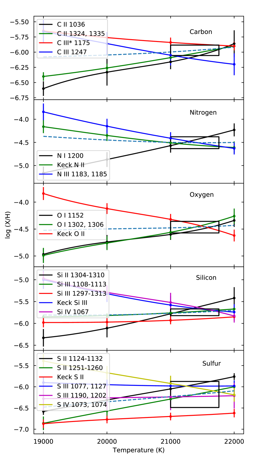
Figure 2: Deriving the effective temperature and abundance of C, N, O, Si, and S. Points with error bars represent the abundance derived from model fits to each absorption feature. Solid lines are low-order polynomial fits to the measured points. Dashed lines represent the weighted mean of the solid lines, computed at 10 K intervals. The black box in each panel denotes the allowed range of temperature and abundance, as described in the text.

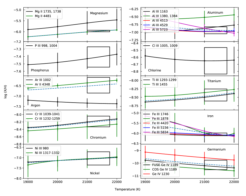
Figure 3: Deriving the abundance of eight additional elements. Points with error bars represent the abundance derived from model fits to each absorption feature. Solid lines are low-order polynomial fits to the measured points. Dashed lines represent the weighted mean of the solid lines, computed at 10 K intervals. The black box in each panel denotes the allowed range of temperature and abundance, as described in the text.

Table 3: Selected Absorption Features in the FUV Spectrum of Barnard 29

Species	Lines Fit (Å)
Carbon	C II 1036.3, 1324.0, 1334.5; C III* 1175 (multiplet); C III 1247.4
Nitrogen	N I 1199.6; N III 1183.0, 1184.5
Oxygen	O I 1152.2, 1302.2, 1306.0
Magnesium	Mg II 1734.9, 1737.6
Aluminum	Al III 1162.6, 1379.7, 1384.1
Silicon	Si II 1304.4, 1309.3, 1309.5
	Si III 1108.4, 1110.0, 1113.2, 1296.7, 1301.1, 1312.6
	Si IV 1066.6
Phosphorus	P III 998.0, 1003.6
Sulfur	S II 1124.4, 1125.0, 1131.1, 1131.7, 1250.6, 1253.8, 1259.5
	S III 1077.1, 1126.5, 1126.9, 1190.2, 1202.1
	S IV 1073.0, 1073.5
Chlorine	Cl III 1005.3, 1008.8
Argon	Ar III 1002.1
Titanium	Ti III 1293.2, 1295.9, 1298.6, 1298.7, 1455.2
Chromium	Cr III 1039–1041, 1231.9, 1233.0, 1236.2, 1238.5, 1247.8, 1252.6, 1259.0
Iron	Fe III 1745.6, 1878.0
Nickel	Ni III 979.6, 1317–1332
Germanium	Ge IV 1189.0, 1229.8

Note. — For chromium and nickel, we fit multiple absorption features in the listed region.

3 Analysis

3.1 Effective Temperature from Ionization Balance

We determine the star’s effective temperature by comparing the absorption features of multiple ionization states of C, N, O, Si, and S. Consider the panel labeled “Nitrogen” in Fig. 2. We fit the COS N I $\lambda 1200$ feature with models (described in Section 3.3) assuming $T_{\rm eff}$ = 19,000 K and find a best-fit value of $\log N({\rm N})/N({\rm H})$ = $-5.16\pm 0.14$. We repeat with models assuming $T_{\rm eff}$ = 20,000 K, 21,000 K, and 22,000 K. The best-fit abundances are plotted as black points and connected with a low-order polynomial (evaluated at 10 K intervals). Vertical bars represent the statistical uncertainties returned by our fitting routine. As the temperature rises, the fraction of nitrogen in the neutral state falls, requiring a higher nitrogen abundance to reproduce the observed feature. Our Keck spectrum exhibits a number of N II lines (Table 2). We fit each of them individually and plot the mean abundance as a function of temperature in green. We fit the N III $\lambda\lambda 1183,1185$ doublet in the FUSE spectrum in the same way and plot the results in blue. (The N III features also appear in the COS spectrum, but they yield abundances with larger error bars, so we use the FUSE values.) As the fraction of ionized nitrogen rises with temperature, the best-fit nitrogen abundance falls.

We repeat this process for C, O, Si, and S, fitting all of the features in the Keck spectrum (Table 2) and selected features in the FUV (Table 3). With few exceptions, the abundance curves intersect between 21,000 K and 22,000 K. To quantify this result, we compute the error-weighted mean abundance and the error-weighted standard deviation as a function of temperature for each element. The mean abundance is plotted as a dashed line in each panel. At each temperature step, we compute

$$\chi^{2}=\sum\Bigl{\{}[y_{i}-y(x_{i})]^{2}/\sigma_{i}^{2}\Bigr{\}},$$

where $y_{i}$ is the abundance derived from a single feature (or group of features; solid line), $y(x_{i})$ is the mean abundance (dashed line), $\sigma_{i}$ is the statistical uncertainty in the derived abundance (vertical bars), and the summation is taken over the 21 abundance curves plotted in Fig. 2. $\chi^{2}$ has a minimum at $T_{\rm eff}$ = 21,400 K. Our lower limit to the temperature is $T_{\rm eff}$ = 21,000 K, set by the point at which $\chi^{2}$ rises by 7.04 relative to its minimum. This choice of $\Delta\chi^{2}$ is strictly correct for a model with six interesting parameters (in our case, one temperature and five abundances) if all errors are normally distributed (Press et al., 1988). For each element, our best-fit abundance is the error-weighted mean value (computed above) at the best-fit temperature. The abundance uncertainty is the larger of the error-weighted standard deviation or the measured uncertainty for the feature that dominates the fit. The black box in each panel denotes the allowed range of temperature and abundance for that element.

Ten other metals, Mg, Al, P, Cl, Ar, Ti, Cr, Fe, Ni, and Ge, exhibit absorption lines in the spectrum of Barnard 28, but only of a single ionization state. (Argon has absorption features from Ar II and Ar III, but the resulting abundance curves do not cross.) We compute their abundances just as for the lighter elements, but do not include them in the calculation of the best-fit temperature. The absorption curves for these species are presented in Fig. 3. The full set of abundances for Barnard 29 is presented in Table 4 and plotted in Fig. 4. Our results are generally consistent with those of Thompson et al. (2007).

Table 4: Photospheric Abundances of Barnard 29, M13, and the Sun

Species	Barnard 29	M13				Sun
		FG	SG	Uncertainty	Scatter
Helium	$-0.89\pm 0.04$	$\cdots$	$\cdots$	$\cdots$	$\cdots$	$-1.07\pm 0.01$
Carbon	$-5.97\pm 0.09$	$-5.55$	$-5.68$	0.14	0.07	$-3.57\pm 0.05$
Nitrogen	$-4.51\pm 0.13$	$-4.89$	$-4.79$	0.13	0.17	$-4.17\pm 0.05$
Oxygen	$-4.46\pm 0.11$	$-4.28$	$-4.71$	0.13	0.17	$-3.31\pm 0.05$
Magnesium	$-5.97\pm 0.04$	$-5.76$	$-5.87$	0.06	0.15	$-4.40\pm 0.04$
Aluminum	$-6.94\pm 0.11$	$-7.09$	$-6.13$	0.13	0.53	$-5.55\pm 0.03$
Silicon	$-5.75\pm 0.08$	$-5.61$	$-5.58$	0.08	0.09	$-4.49\pm 0.03$
Phosphorus	$-7.41\pm 0.14$	$\cdots$	$\cdots$	$\cdots$	$\cdots$	$-6.59\pm 0.03$
Sulfur	$-6.18\pm 0.31$	$\cdots$	$\cdots$	$\cdots$	$\cdots$	$-4.88\pm 0.03$
Chlorine	$-8.65\pm 0.19$	$\cdots$	$\cdots$	$\cdots$	$\cdots$	$-6.50\pm 0.30$
Argon	$-6.47\pm 0.38$	$\cdots$	$\cdots$	$\cdots$	$\cdots$	$-5.60\pm 0.13$
Titanium	$-8.43\pm 0.18$	$-8.42$	$-8.38$	0.16	0.14	$-7.05\pm 0.05$
Chromium	$-8.19\pm 0.15$	$\cdots$	$\cdots$	$\cdots$	$\cdots$	$-6.36\pm 0.04$
Iron	$-6.05\pm 0.07$	$-6.05$	$-6.04$	0.07	0.07	$-4.50\pm 0.04$
Nickel	$-7.03\pm 0.32$	$\cdots$	$\cdots$	$\cdots$	$\cdots$	$-5.78\pm 0.04$
Germanium	$-10.14\pm 0.37$	$\cdots$	$\cdots$	$\cdots$	$\cdots$	$-8.35\pm 0.10$

Note. — Abundances relative to hydrogen: $\log N({\rm X})/N({\rm H})$. M13 values from Mészáros et al. 2015. FG = first generation; SG = second generation. “Uncertainty” represents both random and systematic uncertainties in the derived abundance. “Scatter” represents star-to-star scatter within the cluster. Both value are computed for the entire cluster, rather than either subpopulation. Solar values from Asplund et al. 2009.

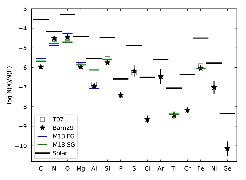
Figure 4: Photospheric abundances of Barnard 29 (from Table 4; stars), the solar photosphere (black lines; Asplund et al. 2009), and the first-generation (FG, blue lines) and second-generation (SG, green lines) stars in M13; Mészáros et al. 2015. Open squares are from fits to the star’s optical spectrum by Thompson et al. 2007.

3.2 Surface Gravity and Helium Abundance

We determine the surface gravity from a simultaneous fit to the star’s Balmer lines (H$\alpha$, H$\beta$, and H$\gamma$). Assuming $T_{\rm eff}$ = 21,400 K, we find that $\log g$ = $3.100\pm 0.003$. This value is not sensitive to small errors in the optical continuum: Repeating the fit using our alternative normalization yields $\log g$ = $3.111\pm 0.003$. Reducing the temperature to 21,000 K yields $\log g$ = $3.071\pm 0.003$; we will adopt this value as the lower limit to the surface gravity. We determine the star’s helium abundance by individually fitting the seven unblended helium features in Table 2. Models assuming our best-fit effective temperature and surface gravity yield a helium abundance of $\log N({\rm He})/N({\rm H})$ = $-0.89\pm 0.04$, where the abundance is the error-weighted mean of our seven results, and the uncertainty is their error-weighted standard deviation. Reducing both the temperature and gravity to their lower limits does not change this result. Our final atmospheric parameters are thus $T_{\rm eff}$ = $21,400\pm 400$ K, $\log g$ = $3.10\pm 0.03$, and $\log N({\rm He})/N({\rm H})$ = $-0.89\pm 0.04$. This model successfully reproduces the hydrogen (Fig. 5) and helium features (Fig. 6) in our HIRES spectrum.

Our metal abundances were derived using models with $\log g$ = 3.0, but our final value is $\log g$ = 3.1. How sensitive are our abundances to this change in the surface gravity? In our fits to the N III $\lambda\lambda 1183,1185$ doublet in the FUSE spectrum, we found $\log N({\rm N})/N({\rm H})$ = $-4.41\pm 0.16$ using models with $T_{\rm eff}$ = 21,000 K and $\log g$ = 3.0. Repeating the fit using models with $\log g$ = 3.1 yields $\log N({\rm N})/N({\rm H})$ = $-4.38\pm 0.15$. The difference is smaller than the uncertainty in any of our abundances.

Using Kurucz (1992) LTE models with [Fe/H] $=-1.0$ and scaled-solar abundances, Conlon et al. (1994) derived stellar parameters of $T_{\rm eff}$ = $20,000\pm 1000$ K, $\log g$ = $3.0\pm 0.1$, and $\log N({\rm He})/N({\rm H})$ = $-1.06\pm 0.20$ for Barnard 29. Thompson et al. (2007) used a grid of NLTE models generated with TLUSTY and SYNSPEC, just as we do, but their models included iron with an abundance [Fe/H] $=-1.1$ and the light elements C, N, O, Mg, Si, and S. They found $T_{\rm eff}$ = $20,000\pm 1000$ K and $\log g$ = $2.95\pm 0.1$. Both groups determined the star’s effective temperature by fitting its Si II and Si III lines and its surface gravity by fitting its H$\gamma$ line. These results are generally consistent with ours. We discuss the use of silicon as temperature indicator in Section 4.1.4.

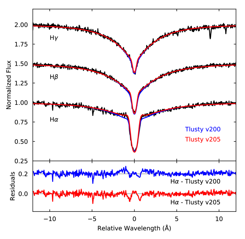
Figure 5: Hydrogen lines in the optical spectrum of Barnard 29 (black). The red curve represents our best-fit synthetic spectrum. It was derived from a stellar atmosphere computed with TLUSTY v205, which employs hydrogen collisional excitation rates taken from Przybilla & Butler 2004. The blue curve was derived from an atmosphere generated with TLUSTY v200, which uses the collisional rates of Mihalas et al. 1975.

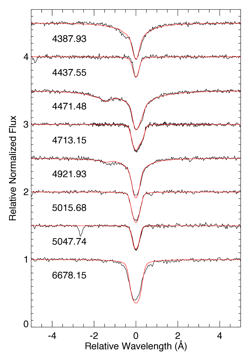
Figure 6: He I lines in the optical spectrum of Barnard 29 (black) with our best-fit synthetic spectrum (red). Two of the lines appear in multiple spectral orders. The line at 6678 Å appears to blended with another feature and is not used to determine the helium abundance.

3.3 Model Atmospheres

We compute a grid of non-local thermodynamic equilibrium (NLTE) stellar-atmosphere models using version 205 of the program TLUSTY (Hubeny & Lanz, 1995). The models are composed of hydrogen, helium, nitrogen, oxygen and the element whose lines we wish to fit. The models have effective temperatures $T_{\rm eff}$ = 19,000, 20,000, 21,000, and 22,000 K; a surface gravity $\log g$ = 3.0; and abundances $\log N({\rm He})/N({\rm H})$ = $-0.9$, $\log N({\rm N})/N({\rm H})$ = $-4.3$, and $\log N({\rm O})/N({\rm H})$ = $-4.5$; these parameters are similar to those derived for Barnard 29 by Thompson et al. (2007). When fitting optical hydrogen and helium lines to determine the surface gravity and helium abundance, we use a grid with surface gravities $\log g$ = 2.8 to 3.2 in steps of 0.1 dex and helium abundances $\log N({\rm He})/N({\rm H})$ = $-1.1$ to $-0.7$ in steps of 0.2 dex. We employ atomic models similar to those used by Lanz & Hubeny (2007) to compute their grid of B-type stars.

From these model atmospheres, we compute synthetic spectra using version 51 of the program SYNSPEC (Hubeny, 1988). For the Keck data, the synthetic spectra are convolved with a Gaussian of FWHM = 0.1 Å to replicate the observed spectrum. For the FUSE data, the synthetic spectra are convolved with a Gaussian of FWHM = 0.06 Å to match the FUSE line-spread function. For the COS G130M spectrum, we model the line-spread function with a Gaussian of FWHM = 0.13 Å. For the G160M spectrum, we employ the tabulated line-spread functions appropriate for data obtained at Lifetime Position #1, which are available from the COS website. For the GHRS spectrum, we adopt a Gaussian with FWHM = 0.095 Å as the line-spread function.

For the elements P, Cl, Ti, Cr, Ni, and Ge, we lack the model atoms necessary to compute full NLTE models. For these species, we adopt an NLTE model atmosphere with a H+He+N+O+Fe composition and compute the ionization fractions of the element in question assuming LTE. We assume $\log N({\rm Fe})/N({\rm H})$ = $-6.0$, which is roughly the cluster abundance. For the iron-peak elements Ti, Cr, and Ni, we can use iron, for which we have a complete set of models, to estimate the abundance errors. To this end, we generate a second grid of iron spectra using the LTE approximation. According to TLUSTY, the dominant ionization state of iron in the stellar photosphere is Fe III. Fitting our LTE models to the star’s Fe III lines yields an abundance consistent with that derived from the NLTE models. Ti III, Cr III, Fe III and Ni III have ionization energies of 27, 31, 31, and 35 eV, respectively, so we expect their populations to vary similarly with temperature.

SYNSPEC computes partition functions for only the first three ionization states of elements heavier than nickel. As a result, there are by default no Ge IV features in our synthetic spectra. To derive an abundance from the star’s Ge IV lines, we must modify the program to include the ionization potentials and partition functions of Ge IV and Ge V. We compute the partition functions by considering all of the statistical weights and energy levels provided by Sugar & Musgrove (1993). The atomic data for the Ge IV 1189 Å and 1230 Å transitions are from Morton (2000).

3.4 Spectral Fitting

Models are fit to the data using a chi-squared minimization routine. Because both the data and the synthetic spectra are normalized, the only free parameter is the abundance of the element in question. Our program linearly interpolates between two model spectra to compute a model with an intermediate abundance. The abundance uncertainties quoted for individual line fits are one-standard deviation errors computed from the covariance matrix returned by the fitting routine; we refer to these as statistical errors.

Continuum placement is the dominant uncertainty in our fits to the FUSE and COS spectra. The FUV spectra of early B-type stars are riddled with absorption lines, and even relatively flat regions of the spectrum are depressed by a myriad of weak absorption features. Allowing our fitting routines to scale the model to the mean level of the “pseudo-continuum” would underestimate the true continuum level. To address this problem, we assume that, at high signal-to-noise ratios, small dips in the spectrum are not noise features, but weak absorption lines, and we normalize the spectrum such that its small-scale features peak at a value of 1.0. To estimate the uncertainty inherent in this technique, we perform each fit twice, once with the model continuum fixed at unity and again with the model scaled by a factor of 0.97, which brings its continuum closer to the pseudo-continuum of the observed spectrum. An example is presented in Fig. 7. The difference in the two abundances is an estimate of the systematic error in our abundance estimates. We add this term and the statistical error in quadrature to compute our final error.

Notes on individual elements:

Magnesium: In the COS spectrum near the Mg II $\lambda\lambda 1734.9,1737.6$ doublet, the continuum is poorly constrained.

Silicon: The Si III 4552.6 Å feature is much stronger than the N II  4552.5 Å line with which it is blended, so we include it in our estimate of the silicon abundance.

Phosphorus: P III has resonance lines at 998.0 and 1003.6 Å, but they lie among a forest of iron and other lines that are not included in our simple models. To limit the effects of blending on the wings of these P III features, we fit only the line cores, a spectral region roughly the width of a single resolution element.

Sulfur: To limit the effects of blending, we fit only the cores of the sulfur lines in the FUSE spectrum.

Chlorine: The Cl III resonance lines at 1005.3, 1008.8, and 1015.0 Å lie in a crowded region of the spectrum, so we fit only the line cores and only the 1005.3 and 1008.8 Å lines.

Argon: In the FUSE spectrum near the Ar III $\lambda 1002$ line, the continuum level is poorly constrained.

Chromium: There are many Cr III lines between 1032 and 1042 Å. Most are blended with other species, but the region between 1039 and 1041 Å contains a half dozen lines that are reasonably well isolated.

Nickel: In the FUSE spectrum near the Ni III $\lambda 980$ line, the continuum level is poorly constrained.

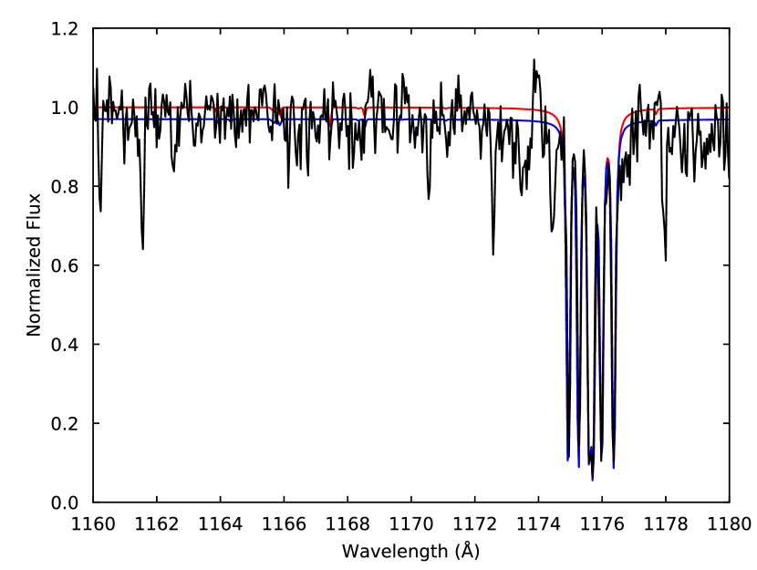
Figure 7: C III* lines in the FUSE spectrum of Barnard 29. The data are normalized as described in the text. The red curve represents a model whose continuum is fixed at 1.0. The blue curve represents a model whose continuum is fixed at 0.97. For this figure, the spectrum has been normalized, binned by three pixels, and shifted to a laboratory wavelength scale.

4 Discussion

4.1 Model Atmospheres

4.1.1 Hydrogen

Our models successfully reproduce the H$\alpha$ line profile, which has a distinctive shape near the line center. To do so, we call TLUSTY with the parameter ICOLHN = 1 (the default value), which triggers the use of hydrogen collisional excitation rates taken from Przybilla & Butler (2004). Older versions of TLUSTY (prior to version 202), which employ the collisional rates of Mihalas et al. (1975), cannot reproduce this feature. In Fig. 5, we plot the best-fit spectra generated with TLUSTY versions 200 (blue) and 205 (red); the red curve better reproduces the line profile. SYNSPEC version 51 offers several sets of hydrogen line profiles. We have experimented with both the Lemke (1997) and Tremblay & Bergeron (2009) profiles and find that the resulting spectra are indistinguishable.

4.1.2 Helium

Careful study of Fig. 6 reveals weak forbidden components in the blue wings of the He I $\lambda 4388$ and $\lambda 4922$ features that are not well reproduced by our model, while a similar component of the He I $\lambda 4471$ feature is well fit. In SYNSPEC, the He I $\lambda 4471$ profile is taken from Barnard, Cooper, & Smith (1974, hereafter BCS74), who provide a set of line profiles for electron densities between $10^{13}$ and $10^{16}$ cm^-3. The profiles of the He I $\lambda 4026$, $\lambda 4388$, and $\lambda 4922$ lines are from Shamey (1969), who gives profiles for electron densities ranging from $10^{14}$ to $3\times 10^{17}$ cm^-3. The line-forming region of our model atmosphere extends to stellar radii with electron densities lower than $10^{14}$ cm^-3, a region of parameter space not included in the Shamey models. Line profiles for the He I $\lambda 4922$ line were computed by Barnard, Cooper, & Smith (1975, hereafter BCS75). Their calculations are based on the work of BCS74 and cover the same range of electron densities. We have incorporated the BCS75 profiles into SYNSPEC. As shown in Fig. 8, the absorption feature at 4920.5 Å is now well reproduced. Unfortunately, line profiles for the He I $\lambda 4388$ line at electron densities lower than $10^{14}$ cm^-3 are not available, preventing us from computing a satisfactory model for this line.

Figure 8: He I $\lambda 4922$ feature in the optical spectrum of Barnard 29 with synthetic spectra generated using line profiles from Shamey 1969 (dotted line) and Barnard et al. 1975 (solid line).

The only He II feature in our data is at 1640.4 Å. We do not use this line when deriving the effective temperature or helium abundance, because the spectrum is rather noisy in this region and the He II line is blended with several metal features. Instead, we simply plot in Fig. 9 the COS spectrum (black curve) and a model with the helium abundance derived from our optical data (red curve). The He II profile is well reproduced by this model.

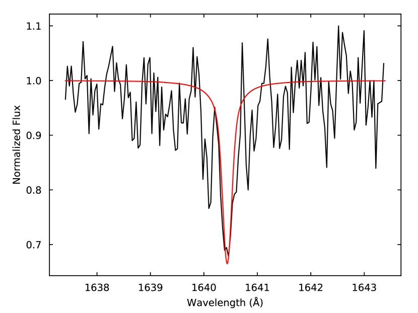
Figure 9: The He II $\lambda 1640$ feature in the COS spectrum of Barnard 29. The red curve is a model with the helium abundance derived from our optical data. For this figure, the spectrum has been normalized, binned by three pixels, and shifted to a laboratory wavelength scale.

4.1.3 Silicon II

Our initial set of model stellar atmospheres employed the silicon model atoms that Lanz & Hubeny (2003, 2007) built to compute their grids of NLTE line-blanketed model atmospheres of B and O stars. The resulting synthetic spectra reproduce the Si III lines in Table 2, but they also predict strong absorption from the Si II features at 5041.0, 5056.0, 5056.3, 6347.1, and 6371.4 Å. Only the 5056.0, 6347.1, and 6371.4 Å lines are observed, and all three are in emission (Fig. 10). In an attempt to alleviate this discrepancy, we employ a more elaborate set of silicon model atoms (retrieved from I. Hubeny’s website) that include additional energy levels and allowed transitions: The new Si II model contains 70 individual energy levels and considers 940 allowed transitions, the Si III model contains 122 levels and considers 1648 transitions, and the Si IV model contains 53 levels and considers 760 transitions. We use these model atoms to generate a new grid of model stellar atmospheres. Fits of the resulting synthetic spectra to the Si III lines yield a lower silicon abundance and weaker Si II absorption (blue curves in Fig. 10). The models do predict faint Si II emission at still lower abundance levels (magenta curves), but the lines weaken as the silicon abundance is further decreased. While our models do not produce Si II emission lines strong enough to match the observed emission, they do explain qualitatively the behavior of the lines by predicting the Si II $\lambda\lambda$5056, 6347, and 6371 lines in emission and the Si II $\lambda$4128.0 line in absorption, as reported by Thompson et al. (2007).

Observations of weak metallic emission lines in the optical spectra of B-type stars have been reported by several authors (e.g., Sigut et al. 2000 and Wahlgren & Hubrig 2000, 2004). In particular, Sadakane & Nishimura (2017) reported the detection of weak Si II $\lambda$6239 and Al II $\lambda$6237 emission in the optical spectra of B-type stars with low rotational velocities. Several of these stars have effective temperatures similar to that of Barnard 29, but their gravities are higher by 0.6 to 1.1 dex. They are also significantly more metal rich. The Si II $\lambda$6239 line is not observed in the spectrum of Barnard 29 because of the star’s low silicon abundance; however, by raising the silicon abundance of our models to $\log N({\rm Si})/N({\rm H})$ = $-4.80$, we can generate synthetic spectra with the Si II $\lambda$6239 line in emission and the Si II $\lambda\lambda 5056.0,$ 6347.1, and 6371.4 lines in absorption, reproducing the pattern seen by Sadakane & Nishimura. This result strengthens our confidence in these models and demonstrates that variations in the silicon abundance can explain, at least qualitatively, the pattern in the Si II lines that is observed in both Barnard 29 and some of the B-type stars analyzed by Sadakane & Nishimura.

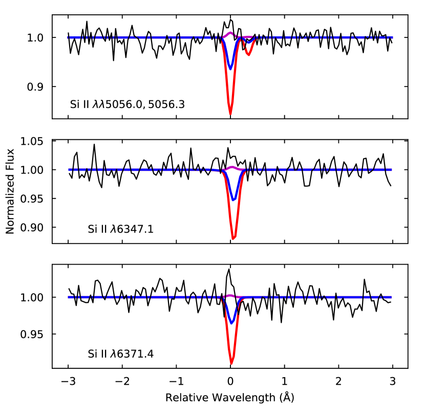
Figure 10: Si II emission in the HIRES spectrum of Barnard 29. The red curve represents our initial fit to the observed Si III features, which yields $\log N({\rm Si})/N({\rm H})$ = $-5.12$. At this abundance, the Si II lines are predicted to be strong absorption features. The blue curve represents a second model, using more sophisticated silicon model atoms, also fit to the Si III features. With an abundance of $\log N({\rm Si})/N({\rm H})$ = $-5.57$, this model predicts weaker Si II absorption. If we further reduce the abundance, we find that these lines go into emission at abundances lower than $\log N({\rm Si})/N({\rm H})$ = $-5.80$; the emission reaches a maximum around $\log N({\rm Si})/N({\rm H})$ = $-6.4$ (magenta curve).

4.1.4 Silicon III

Conlon et al. (1994) derived an effective temperature of $T_{\rm eff}$ $=20,000\pm 1000$ K by requiring that the Si II line at 4128 Å and the Si III triplet at 4552, 4567, and 4574 Å yield consistent silicon abundances. Thompson et al. (2007) employed the same technique (with the addition of Si III $\lambda 5739$) and achieved the same result. Our equilibrium analysis includes these Si III lines, yet yields an effective temperature of 21,400 K. Why might that be? In Fig. 11 we plot the abundances derived from each of the Si III features in our Keck spectrum. We cannot model our Si II lines, so we use the equivalent width of the Si II $\lambda 4128$ line published by Thompson et al. to derive a silicon abundance. We see that the Si II curve crosses those for the Si III triplet at $T_{\rm eff}$ $\sim 20,500$ K, while it crosses the curve for Si III $\lambda 5739$ at $T_{\rm eff}$ $\sim 21,300$ K. This plot is derived from models using oscillator strengths from Kurucz (1992); models using oscillator strengths from the more recent compliation of Kelleher & Podobedova (2008) show an even greater difference ($\sim 1000$ K) between the intersection points. Apparently, the Si III triplet yields systematically lower abundances than does Si III $\lambda 5739$, leading to a lower effective temperature from an equilibrium analysis. The Keck Si III curve in Fig. 2 represents the mean of the four Si III curves shown here.

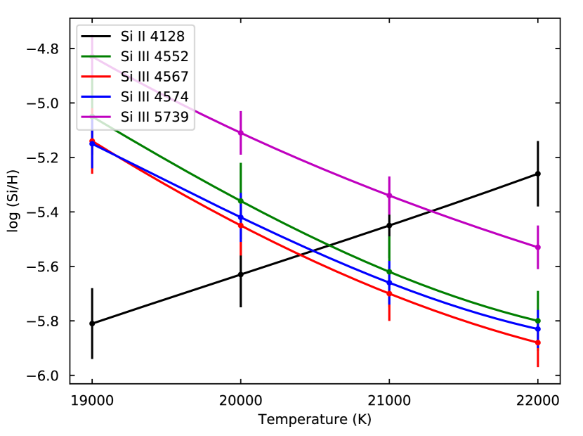
Figure 11: Deriving the effective temperature from silicon lines in the optical spectrum of Barnard 29. The Si II curve is computed from the equivalent width of Si II $\lambda 4128$ published by Thompson et al. 2007. The Si III curves are derived from features in our Keck spectrum. Points with error bars represent the abundance derived from model fits to each absorption feature. Solid lines are low-order polynomial fits to the measured points.

4.1.5 Microturbulence

Microturbulence is an ad hoc parameter originally introduced to reconcile discrepancies between theoretical and empirical curves of growth (Mihalas, 1978). In a traditional abundance analysis based on absorption-line equivalent widths, the microturbulent velocity $\xi$ is adjusted to remove any trend in abundance for individual atomic transitions as a function of the lower excitation potential or line strength. In practical terms, microturbulence corrects for (or obscures) deficiencies in plane-parallel atmospheric models, including errors in the treatment of collisional broadening, dynamical effects, inhomogeneities, and non-LTE effects.

In calculating our atmospheric models, we have set $\xi=0$ km s^-1. To explore the implications of this decision, we calculate a second set of models assuming $\xi=4$ km s^-1, the value adopted by Thompson et al. (2007), and compare them to the data. The top row of Fig. 12 shows a set of nitrogen and oxygen features fit to the Keck spectrum using models with $\xi=0$ km s^-1. For this figure, each line is fit independently, and the resulting abundance is listed. The bottom row shows the same features fit using models with $\xi=4$ km s^-1. While the abundances are little changed, the quality of the fit is obviously poorer, as evidenced by the increase in $\chi^{2}$. We conclude that the data are best reproduced by models with $\xi=0$ km s^-1.

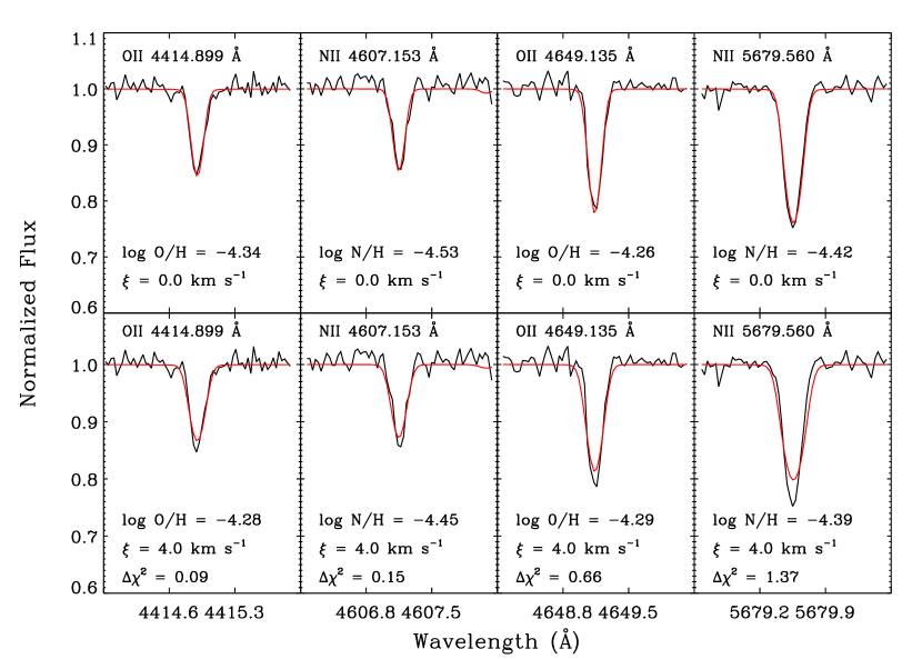
Figure 12: Top row: Nitrogen and oxygen features from the Keck spectrum of Barnard 29 fit using models with $\xi=0$ km s^-1. Bottom row: The same features fit using models with $\xi=4$ km s^-1.

4.2 Photospheric Abundances

Galactic globular clusters host multiple stellar populations. First-generation (FG) stars display abundances typical of halo field stars, while second-generation (SG) stars, which may have multiple subpopulations, are enriched in Na and Al and depleted in O and Mg. Models suggest that the second generation is formed from gas polluted by material expelled by massive stars of the first generation. (For details, see the review by Bastian & Lardo 2018.) Mészáros et al. (2015) identified two stellar populations on the RGB of M13. FG stars (blue lines in Fig. 4) are richer in O and poorer in Al than SG stars (green lines). Barnard 29 is clearly a FG star, richer in O and poorer in Al. The star is depleted in C and enhanced in N; otherwise, its abundances appear to have changed little since it left the RGB. In particular, its low carbon abundance ($N_{C}/N_{O}=0.03$) indicates that the star did not undergo third dredge-up.

In addition to the abundance trends attributable to multiple populations, Mészáros et al. (2015) find a clear correlation in the abundance of carbon with effective temperature in M13. The authors interpret this trend as a sign of “deep mixing,” a nonconvective mixing process that results in a steady depletion of the surface carbon abundance and an enhancement in the nitrogen abundance in low-mass stars as they evolve up the RGB (Gratton et al., 2004). The abundance pattern seen in Barnard 29 — C depletion and N enhancement relative to the average value for FG stars on the RGB — suggests that the star experienced the full impact of deep mixing.

4.2.1 Iron Abundance

The iron abundance of Barnard 29 has been a puzzlement for more than two decades. Conlon et al. (1994) set an upper limit of $\log N({\rm Fe})/N({\rm H})$ $<-5.30\pm 0.30$ from an optical spectrum of the star. Dixon & Hurwitz (1998) observed Barnard 29 with the Berkeley Spectrometer, which spans the same wavelength range as FUSE, but at lower resolution. Fitting spectra derived from Kurucz (1992) models to the region between 1115 and 1160 Å, they derived $\log N({\rm Fe})/N({\rm H})$ = $-6.70^{+0.22}_{-0.26}$. Both Moehler et al. (1998) and Thompson et al. (2007) modeled the star’s GHRS spectrum, deriving $\log N({\rm Fe})/N({\rm H})$ = $-6.79\pm 0.10$ and $\log N({\rm Fe})/N({\rm H})$ = $-6.6\pm 0.1$, respectively. All of these FUV-derived values are significantly lower than the cluster iron abundance of $\log N({\rm Fe})/N({\rm H})$ = $-6.05$ (Mészáros et al., 2015). Strangely, Thompson et al. found that fits to the star’s optical spectrum yield $\log N({\rm Fe})/N({\rm H})$ $-5.93\pm 0.12$, a value consistent with the cluster metallicity. Canonical stellar-evolution theory predicts no evolutionary changes in the iron abundance of low-mass stars like those in Galactic globular clusters today (Iben & Renzini, 1983).

We have independently derived the iron abundance of Barnard 29 from its Keck, FUSE, COS, and GHRS spectra. Our values are consistent with one another (Fig. 3) and with the cluster iron abundance (Fig. 4). To understand the difference between our results and those of previous authors, we have conducted a series of numerical experiments, systematically testing the assumptions made by Moehler et al. (1998). Following them, we fit the entire suite of Fe III features in the GHRS spectrum. Using models with a microturbulent velocity $\xi=0$ km s^-1, we derive an iron abundance $\log N({\rm Fe})/N({\rm H})$ = $-6.16\pm 0.16$. Moehler et al. adopt the value $\xi=10$ km s^-1 derived by Conlon et al. (1994). Using models with $\xi=10$ km s^-1, we derive an iron abundance $\log N({\rm Fe})/N({\rm H})$ = $-6.79\pm 0.09$, which matches the Moehler et al. result. Assuming a spectral resolution of FHWM = 0.07 Å, employing LTE models, or adopting the atomic data presented by Moehler et al. does not further reduce the derived iron abundance.

Abundances derived from FUV spectra are sensitive to the assumed value of the microturbulent velocity. Many FUV lines are saturated, and over-estimating the microturbulence results in an under-estimate of the abundance. Conlon et al. (1994) derive $\xi=10\pm 2$ km s^-1 by minimizing the scatter in the abundance derived from 17 oxygen lines in the star’s optical spectrum. Dixon & Hurwitz (1998) employ Kurucz models with $\xi=2$ km s^-1, while Thompson et al. (2007) derive $\xi=4\pm 2$ km s^-1 from fits to O II and Si III lines.

4.2.2 Zirconium Abundance

In a preliminary analysis of the FUSE and COS data (Dixon et al., 2011), we attributed the strong absorption feature at 1184 Å to Zr IV; however, recent calculations of Zr IV oscillator strengths by Rauch et al. (2017) raise doubts about this identification. Zr IV $\lambda 1184$ should be accompanied by Zr IV $\lambda 1220$, as both are resonance transitions, yet the $\lambda 1220$ feature is not seen. The hot sub-dwarf B star CPD$-64$ 481 has an effective temperature $T_{\rm eff}$ = 27,500 K (O’Toole et al., 2005), similar to that of Barnard 29. Examination of a high-resolution spectrum of CPD$-64$ 481 obtained with the HST STIS E140H grating reveals that Zr IV $\lambda 1184$ is blended with another, unidentified feature. We conclude that the 1184 Å feature cannot be used to derive the Zr abundance of stars observed at the resolution of FUSE or COS.

4.3 Stellar Mass and Luminosity

We can derive a star’s radius, and from this its mass and luminosity, by comparing its observed and predicted flux. The spectral irradiance of Barnard 29 has been measured in several bands: $B=12.934$, $V=13.116$, $I=13.303$ mag (Sandquist et al., 2010), for which we assume an uncertainty of 0.003 mag. The extinction toward M13 is E(B V) = $0.02\pm 0.01$ mag (Harris, 2010). We model the stellar continuum using an NLTE model, similar to the H+He+N+O+Fe models described in Section 3.3 but with our best-fit atmospheric parameters, scaled by a Cardelli et al. (1989) extinction curve with $R_{V}=3.1$. We compute synthetic stellar magnitudes using the Python package Pysynphot (Lim et al., 2015), adjusting the magnitude zero points as described by Dixon et al. (2017). The data are best fit with a scale factor $\phi=(1.216\pm 0.002)\times 10^{-21}$. We repeat the fit assuming an extinction E(B V) = 0.03 and get $\phi=(1.251\pm 0.002)\times 10^{-21}$. Combining this change with the statistical error yields a final scale factor $\phi=(1.22\pm 0.04)\times 10^{-21}$.

In the synthetic spectra generated by SYNSPEC, the flux is expressed in terms of the flux moment, $H_{\lambda}$. If the star’s radius and distance are known, then the scale factor required to convert the model to the flux at earth is $\phi=4\pi(R_{*}/d)^{2}$ (Kurucz, 1979). Unfortunately, we cannot use results from Gaia Data Release 2 to constrain the distance to M13, as Gaia globular-cluster parallaxes suffer from significant systematic errors (Helmi et al., 2018). Recent published values range from 7.1 kpc (Harris, 2010) to 7.9 kpc (O’Malley et al., 2017). Adopting this distance range and our scale factor, we derive a stellar radius $R_{*}/R_{\sun}$ between 3.11 and 3.45. Applying our best-fit surface gravity ($\log g$ = 3.1), we find that the stellar mass $M_{*}/M_{\sun}$ is between 0.45 and 0.55. Finally, combining the stellar radius with our best-fit effective temperature ($T_{\rm eff}$ = 21,400 K), we derive a stellar luminosity $\log L_{*}/L_{\sun}$ between 3.26 and 3.35, slightly greater than the range $\log L_{*}/L_{\sun}$ = 3.08 – 3.25 estimated by Conlon et al. (1994). All derived values (radius, mass, and luminosity) scale with the cluster distance.

4.4 Evolutionary Status

The post-HB evolution of M13 stars is illustrated in Fig. 13. The coolest ($T_{\rm eff}$ $\lesssim$ 8,000 K), most massive ($M_{\rm ZAHB}\gtrsim 0.70M_{\sun}$) stars populate the red horizontal branch (RHB, red points). As they depart the HB, they evolve to the red and ascend the AGB. Stars on the blue horizontal branch (BHB, blue points) are hotter (8,000 K $\lesssim$ $T_{\rm eff}$ $\lesssim$ 20,000 K) and have lower masses ($0.52\lesssim M_{\rm ZAHB}\lesssim 0.70M_{\sun}$). Most post-BHB stars also climb the AGB and reach the thermal-pulsing AGB phase, but only for a short time. The hottest ($T_{\rm eff}$ $\gtrsim$ 20,000 K), least-massive ($M_{\rm ZAHB}\lesssim 0.52M_{\sun}$) stars populate the extreme horizontal branch (EHB, cyan points). Most of these stars do not climb the AGB after the He-core burning phase, but evolve to high luminosities with little change in temperature. Post-EHB stars are also known as AGB-manqué stars. Stars near the boundary between the EHB and the BHB ($T_{\rm eff}$ $\sim$ 20,000 K, $M_{\rm ZAHB}\sim 0.52M_{\sun}$) follow an intermediate path: they climb the AGB, but depart before reaching the thermal-pulsing phase, becoming post-early AGB (post-EAGB) stars.

The tracks plotted in Fig. 13 represent an extension of the work presented by Miller Bertolami (2016). The models are computed for [Fe/H] = $-1.5$ and a zero-age main-sequence (ZAMS) mass of $M_{\rm ZAMS}=0.83$ $M_{\sun}$ (age 11.7 Gyr), assuming a scaled-solar metal content with initial abundances $Z_{\rm ZAMS}=0.000548$, $Y_{\rm ZAMS}=0.246096$, and $X_{\rm ZAMS}=0.753356$. Winds on the RGB are adjusted to populate the extreme, blue, and red horizontal branches. Zero-age horizontal-branch (ZAHB) masses are $M_{\rm ZAHB}=0.83$, 0.75 and 0.70 $M_{\sun}$ (final masses $M_{\rm WD}=0.557$, 0.550, and 0.540$M_{\sun}$) for the RHB (red points); $M_{\rm ZAHB}=0.65$, 0.60, 0.55, and 0.53 $M_{\sun}$ (final masses $M_{\rm WD}=0.525$, 0.519, 0.505, and 0.501 $M_{\sun}$) for the BHB (blue points); and $M_{\rm ZAHB}=0.51$, 0.50, and 0.495 $M_{\sun}$ (final masses $M_{\rm WD}=0.500$, 0.499, and 0.495 $M_{\sun}$) for the EHB (cyan points). The dark-cyan points show the evolution of the hottest possible post-EHB model. This sequence corresponds to a Late Hot-Flasher sequence (see Battich et al. 2018 for a detailed explanation) that undergoes a violent H-burning event during the He-core flash and ends as a H-deficient ZAHB model (surface abundances [H, He, C, N] = [$2.3\times 10^{-4}$, 0.9636, 0.024, 0.012] by mass fraction), with a ZAHB mass of $M_{\rm ZAHB}=0.49$ $M_{\sun}$ (final mass $M_{\rm WD}=0.489$ $M_{\sun}$).

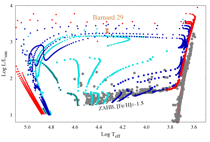
Figure 13: Evolutionary tracks for stars similar to those of M13 during and after the horizontal-branch stage. Colors indicate stars that spend their core helium burning stage as Red Horizontal Branch stars (red), Blue Horizontal Branch stars (blue), and Extreme Horizontal Branch Stars (cyan). The hottest track (dark cyan) represents a Late Hot-Flasher sequence. Circles are plotted every 10 Myr, squares are plotted every 1 Myr, and diamonds indicate intervals of 20,000 yr. The vertical orange bar marks the effective temperature and range of allowed luminosities for Barnard 29.

To these evolutionary tracks we have added a sample of M13 stars from Nardiello et al. (2018), who provide a five-band catalog of stellar magnitudes from the HST UV Legacy Survey of Galactic Globular Clusters (Piotto et al., 2015) and the ACS Globular Cluster Survey (Sarajedini et al., 2007). Effective temperatures are estimated from F275W $-$ F438W colors, and luminosities from F606W magnitudes. We use Castelli & Kurucz (2003) models with [Fe/H] = $-1.5$ to determine these relationships. The cluster distance and reddening are taken from Harris (2010). Barnard 29 is indicated by a vertical orange bar that spans the range of luminosities derived in Section 4.3.

M13 hosts only a handful of RHB stars, but its BHB and EHB are well populated. In Fig. 13, we see a number of hot stars more luminous than the HB. Some appear to be following the post-BHB tracks toward the AGB, and some the post-EHB tracks toward the white-dwarf cooling curve. Sandquist et al. (2010) estimate that roughly one-third of the post-HB stars in M13 are on post-EHB tracks.

The derived mass and luminosity of Barnard 29 depend on its distance. If M13 lies at the low end of the allowed range ($d\sim 7.1$ kpc), then $M_{*}/M_{\sun}\sim 0.45$ and $\log L_{*}/L_{\sun}\sim 3.26$. These values have interesting implications for the star’s evolutionary history. No HB star can have a mass less than 0.49 $M_{\sun}$, because core helium ignition is impossible at such low masses. An evolved star with $M_{*}/M_{\sun}<0.49$ must have experienced extreme mass loss on the RGB (more even than the cluster’s EHB stars), left the RGB before the helium-core flash, and is now evolving directly from the RGB to the white-dwarf cooling curve, where it will become a helium-core white dwarf. The fact that M13 has a large population of extreme EHB stars suggests that it may also have a population of lower-mass post-RGB stars, because a finely-tuned mass-loss process would be required to remove just enough material from RGB stars to produce a large population of the hottest EHB stars without creating any lower-mass objects. So it is not unthinkable that Barnard 29 is a post-RGB star. On the other hand, only the most massive post-RGB stars would be as luminous as Barnard 29. According to stellar-evolution models, a post-RGB star with the luminosity of Barnard 29 would have a mass $M_{*}/M_{\sun}=0.48$, greater than the derived value for this distance. Consequently, a post-RGB origin for Barnard 29 is unlikely.

If the cluster lies at the high end of the allowed range ($d\sim 7.9$ kpc), then $M_{*}/M_{\sun}\sim 0.55$ and $\log L_{*}/L_{\sun}\sim 3.35$, values consistent with the star’s being a post-BHB star. At an intermediate distance, the mass of Barnard 29 would lie between these extremes; values $M_{*}/M_{\sun}\lesssim 0.52$ would place the star on one of the post-EHB evolutionary tracks. We can exclude the hottest EHB track in Fig. 13, which yields a white dwarf with mass around 0.495 $M_{\sun}$. It traces the path of AGB-manqué stars that evolve directly from the HB to the white-dwarf cooling curve. Barnard 29 is clearly cooler and more luminous than this track, suggesting a mass $M_{*}/M_{\sun}\gtrsim 0.5$.

In light of stellar-evolution models, it seems likely that Barnard 29 is a post-HB star evolving from a ZAHB star with $M_{\rm ZAHB}$ between 0.50 and 0.55 $M_{\sun}$, a range spanning the EHB/BHB boundary. A post-HB star would have fully ascended the RGB, consistent with our suggestion that Barnard 29 experienced the full effects of nonconvective mixing on the RGB. Its relatively low mass is consistent with our conclusion that the star did not experience third dredge-up.

5 Summary and Conclusions

We have performed a spectral analysis of the UV-bright star Barnard 29 in M13. By requiring multiple ionization states of C, N, O, Si, and S to yield consistent abundances, we derive an effective temperature $T_{\rm eff}$ = $21,400\pm 400$ K. We derive a surface gravity $\log g$ = $3.10\pm 0.03$ from the star’s Balmer lines. Using the latest version of TLUSTY, we are able to reproduce the observed H$\alpha$ profile. By adding He I line profiles to SYNSPEC, we reproduce the absorption feature at 4920.5 Å. Although our models predict faint Si II emission in the optical, they cannot reproduce the strength of the observed features. We derive the photospheric abundances of He, C, N, O, Mg, Al, Si, P, S, Cl, Ar, Ti, Cr, Fe, Ni, and Ge. Barnard 29 exhibits an abundance pattern typical of first-generation stars in M13, though an underabundance of C and an overabundance of N suggest that the star experienced nonconvective mixing on the RGB. This pattern appears to have changed little since the star left the RGB. In particular, the star did not undergo third dredge-up. Previous workers have found that the star’s FUV spectra yield an iron abundance about 0.5 dex lower than its optical spectrum. The iron abundances derived from our Keck, FUSE, COS, and GHRS spectra are consistent with one another and with the cluster value. We attribute the difference to our use of model atmospheres without microturbulence, which is ruled out by the quality of the fits to the optical N II and O II lines. Barnard 29 lies in a region of the temperature-luminosity plane that is traversed by both post-BHB and post-EHB evolutionary tracks. Comparison with stellar-evolution models suggests that it evolved from a ZAHB star of mass $M_{*}/M_{\sun}$ between 0.50 and 0.55, close to the EHB/BHB boundary.

References

- Asplund et al. (2009) Asplund, M., Grevesse, N., Sauval, A. J., & Scott, P. 2009, ARA&A, 47, 481, doi: 10.1146/annurev.astro.46.060407.145222
- Barnard et al. (1974) Barnard, A. J., Cooper, J., & Smith, E. W. 1974, J. Quant. Spec. Radiat. Transf., 14, 1025, doi: 10.1016/0022-4073(74)90085-5
- Barnard et al. (1975) —. 1975, J. Quant. Spec. Radiat. Transf., 15, 429, doi: 10.1016/0022-4073(75)90062-X
- Barnard (1900) Barnard, E. E. 1900, ApJ, 12, 176, doi: 10.1086/140754
- Barnard (1909) —. 1909, ApJ, 29, 72, doi: 10.1086/141621
- Barnard (1914) —. 1914, ApJ, 40, 173, doi: 10.1086/142108
- Bastian & Lardo (2018) Bastian, N., & Lardo, C. 2018, ARA&A, 56, 83, doi: 10.1146/annurev-astro-081817-051839
- Battich et al. (2018) Battich, T., Miller Bertolami, M. M., Córsico, A. H., & Althaus, L. G. 2018, A&A, 614, A136, doi: 10.1051/0004-6361/201731463
- Cardelli et al. (1989) Cardelli, J. A., Clayton, G. C., & Mathis, J. S. 1989, ApJ, 345, 245, doi: 10.1086/167900
- Castelli & Kurucz (2003) Castelli, F., & Kurucz, R. L. 2003, in IAU Symp. 210, Modelling of Stellar Atmospheres, ed. N. Piskunov, W. W. Weiss, & D. F. Gray (San Francisco: ASP), A20
- Conlon et al. (1994) Conlon, E. S., Dufton, P. L., & Keenan, F. P. 1994, A&A, 290, 897
- Dixon et al. (2017) Dixon, W. V., Chayer, P., Latour, M., Miller Bertolami, M. M., & Benjamin, R. A. 2017, AJ, 154, 126, doi: 10.3847/1538-3881/aa8450
- Dixon et al. (2011) Dixon, W. V., Chayer, P., Welsh, B. Y., & Green, J. C. 2011, BAAS, 43, 338.15
- Dixon & Hurwitz (1998) Dixon, W. V., & Hurwitz, M. 1998, ApJ, 500, L29, doi: 10.1086/311391
- Dixon et al. (2007) Dixon, W. V., Sahnow, D. J., Barrett, P. E., et al. 2007, PASP, 119, 527, doi: 10.1086/518617
- Fox (2015) Fox, A. J. 2015, COS Data Handbook, Version 3.0 (Baltimore: STScI)
- Gratton et al. (2004) Gratton, R., Sneden, C., & Carretta, E. 2004, ARA&A, 42, 385, doi: 10.1146/annurev.astro.42.053102.133945
- Green et al. (2012) Green, J. C., Froning, C. S., Osterman, S., et al. 2012, ApJ, 744, 60, doi: 10.1088/0004-637X/744/1/60
- Harris (1996) Harris, W. E. 1996, AJ, 112, 1487, doi: 10.1086/118116
- Harris (2010) —. 2010, ArXiv e-prints. https://arxiv.org/abs/1012.3224
- Heap et al. (1995) Heap, S. R., Brandt, J. C., Randall, C. E., et al. 1995, PASP, 107, 871, doi: 10.1086/133635
- Helmi et al. (2018) Helmi, A., van Leeuwen, F., McMillan, P., et al. 2018, A&A, 616, A12, doi: 10.1051/0004-6361/201832698
- Hubeny (1988) Hubeny, I. 1988, CoPhC, 52, 103, doi: 10.1016/0010-4655(88)90177-4
- Hubeny & Lanz (1995) Hubeny, I., & Lanz, T. 1995, ApJ, 439, 875, doi: 10.1086/175226
- Iben & Renzini (1983) Iben, Jr., I., & Renzini, A. 1983, ARA&A, 21, 271, doi: 10.1146/annurev.aa.21.090183.001415
- Kelleher & Podobedova (2008) Kelleher, D., & Podobedova, L. 2008, JPCRD, 37, 1285, doi: 10.1063/1.2734566
- Kurucz (1979) Kurucz, R. L. 1979, ApJS, 40, 1, doi: 10.1086/190589
- Kurucz (1992) Kurucz, R. L. 1992, in IAU Symp. 149, The Stellar Populations of Galaxies, ed. B. Barbuy & A. Renzini (Dordrecht: Kluwer), 225. http://adsabs.harvard.edu/cgi-bin/nph-bib_query?bibcode=1992IAUS..149..225K&db_key=AST
- Lanz & Hubeny (2003) Lanz, T., & Hubeny, I. 2003, ApJS, 146, 417, doi: 10.1086/374373
- Lanz & Hubeny (2007) —. 2007, ApJS, 169, 83, doi: 10.1086/511270
- Lehner et al. (2004) Lehner, N., Wakker, B. P., & Savage, B. D. 2004, ApJ, 615, 767, doi: 10.1086/424730
- Lemke (1997) Lemke, M. 1997, A&AS, 122, 285, doi: 10.1051/aas:1997134
- Lim et al. (2015) Lim, P. L., Diaz, R. I., & Laidler, V. 2015, PySynphot User’s Guide (Baltimore: STScI)
- Mészáros et al. (2015) Mészáros, S., et al. 2015, AJ, 149, 153, doi: 10.1088/0004-6256/149/5/153
- Mihalas (1978) Mihalas, D. 1978, Stellar Atmospheres (San Francisco: Freeman), 323. http://adsabs.harvard.edu/cgi-bin/nph-bib_query?bibcode=1978stat.book.....M&db_key=AST
- Mihalas et al. (1975) Mihalas, D., Heasley, J. N., & Auer, L. H. 1975, A Non-LTE Model Stellar Atmosphere Computer Program, NCAR-TN/STR-104
- Miller Bertolami (2016) Miller Bertolami, M. M. 2016, A&A, 588, A25, doi: 10.1051/0004-6361/201526577
- Moehler et al. (1998) Moehler, S., Heber, U., Lemke, M., & Napiwotzki, R. 1998, A&A, 339, 537
- Moos et al. (2000) Moos, H. W., Cash, W. C., Cowie, L. L., et al. 2000, ApJ, 538, L1, doi: 10.1086/312795
- Morton (2000) Morton, D. C. 2000, ApJS, 130, 403, doi: 10.1086/317349
- Nardiello et al. (2018) Nardiello, D., Libralato, M., Piotto, G., et al. 2018, MNRAS, 481, 3382, doi: 10.1093/mnras/sty2515
- O’Malley et al. (2017) O’Malley, E. M., Gilligan, C., & Chaboyer, B. 2017, ApJ, 838, 162, doi: 10.3847/1538-4357/aa6574
- O’Toole et al. (2005) O’Toole, S. J., Jordan, S., Friedrich, S., & Heber, U. 2005, A&A, 437, 227, doi: 10.1051/0004-6361:20042554
- Piotto et al. (2015) Piotto, G., Milone, A. P., Bedin, L. R., et al. 2015, AJ, 149, 91, doi: 10.1088/0004-6256/149/3/91
- Press et al. (1988) Press, W. H., Flannery, B. P., Teukolsky, S. A., & Vetterling, W. T. 1988, Numerical Recipes in C: The Art of Scientific Computing (Cambridge: Cambridge Univ. Press)
- Przybilla & Butler (2004) Przybilla, N., & Butler, K. 2004, ApJ, 609, 1181, doi: 10.1086/421316
- Rauch et al. (2017) Rauch, T., Gamrath, S., Quinet, P., et al. 2017, A&A, 599, A142, doi: 10.1051/0004-6361/201629794
- Sadakane & Nishimura (2017) Sadakane, K., & Nishimura, M. 2017, Publications of the Astronomical Society of Japan, 69, 48, doi: 10.1093/pasj/psx024
- Sahnow et al. (2000) Sahnow, D. J., Moos, H. W., Ake, T. B., et al. 2000, ApJ, 538, L7, doi: 10.1086/312794
- Sandquist et al. (2010) Sandquist, E. L., Gordon, M., Levine, D., & Bolte, M. 2010, AJ, 139, 2374, doi: 10.1088/0004-6256/139/6/2374
- Sarajedini et al. (2007) Sarajedini, A., Bedin, L. R., Chaboyer, B., et al. 2007, AJ, 133, 1658, doi: 10.1086/511979
- Shamey (1969) Shamey, P. 1969, PhD thesis, University of Colorado
- Sigut et al. (2000) Sigut, T. A. A., Landstreet, J. D., & Shorlin, S. L. S. 2000, ApJ, 530, L89, doi: 10.1086/312499
- Smith (2005) Smith, G. H. 2005, The Observatory, 125, 244
- Soderblom et al. (1995) Soderblom, D. R., Gonnella, A., Hulbert, S. J., et al. 1995, Instrument Handbook for the Goddard High-Resolution Spectrograph, Version 6.0 (Baltimore: STScI)
- Sugar & Musgrove (1993) Sugar, J., & Musgrove, A. 1993, Journal of Physical and Chemical Reference Data, 22, 1213, doi: 10.1063/1.555929
- Thompson et al. (2007) Thompson, H. M. A., Keenan, F. P., Dufton, P. L., et al. 2007, MNRAS, 378, 1619, doi: 10.1111/j.1365-2966.2007.11916.x
- Tremblay & Bergeron (2009) Tremblay, P.-E., & Bergeron, P. 2009, ApJ, 696, 1755, doi: 10.1088/0004-637X/696/2/1755
- Vogt et al. (1994) Vogt, S. S., et al. 1994, in Proc. SPIE, Vol. 2198, Instrumentation in Astronomy VIII, ed. D. L. Crawford & E. R. Craine, 362
- Wahlgren & Hubrig (2000) Wahlgren, G. M., & Hubrig, S. 2000, A&A, 362, L13
- Wahlgren & Hubrig (2004) —. 2004, A&A, 418, 1073, doi: 10.1051/0004-6361:20034257
- Welsh et al. (2011) Welsh, B. Y., Wheatley, J., & Lallement, R. 2011, PASP, 123, 914, doi: 10.1086/661604
- White et al. (2016) White, J., De Rosa, G., Plesha, R., & Sahnow, D. 2016, Characterizing the COS OSM1 Drift in the Dispersion Direction, ISR COS 2016-2 (Baltimore: STScI)