Transformation-consistent Self-ensembling Model for Semi-supervised Medical Image Segmentation

Abstract

A common shortfall of supervised deep learning for medical imaging is the lack of labeled data, which is often expensive and time-consuming to collect. This paper presents a new semi-supervised method for medical image segmentation, where the network is optimized by a weighted combination of a common supervised loss only for the labeled inputs and a regularization loss for both the labeled and unlabeled data. To utilize the unlabeled data, our method encourages consistent predictions of the network-in-training for the same input under different perturbations. With the semi-supervised segmentation tasks, we introduce a transformation-consistent strategy in the self-ensembling model to enhance the regularization effect for pixel-level predictions. To further improve the regularization effects, we extend the transformation in a more generalized form including scaling and optimize the consistency loss with a teacher model, which is an averaging of the student model weights. We extensively validated the proposed semi-supervised method on three typical yet challenging medical image segmentation tasks: (i) skin lesion segmentation from dermoscopy images in the International Skin Imaging Collaboration (ISIC) 2017 dataset, (ii) optic disc segmentation from fundus images in the Retinal Fundus Glaucoma Challenge (REFUGE) dataset, and (iii) liver segmentation from volumetric CT scans in the Liver Tumor Segmentation Challenge (LiTS) dataset. Compared to state-of-the-art, our method shows superior performance on the challenging 2D/3D medical images, demonstrating the effectiveness of our semi-supervised method for medical image segmentation.

I Introduction

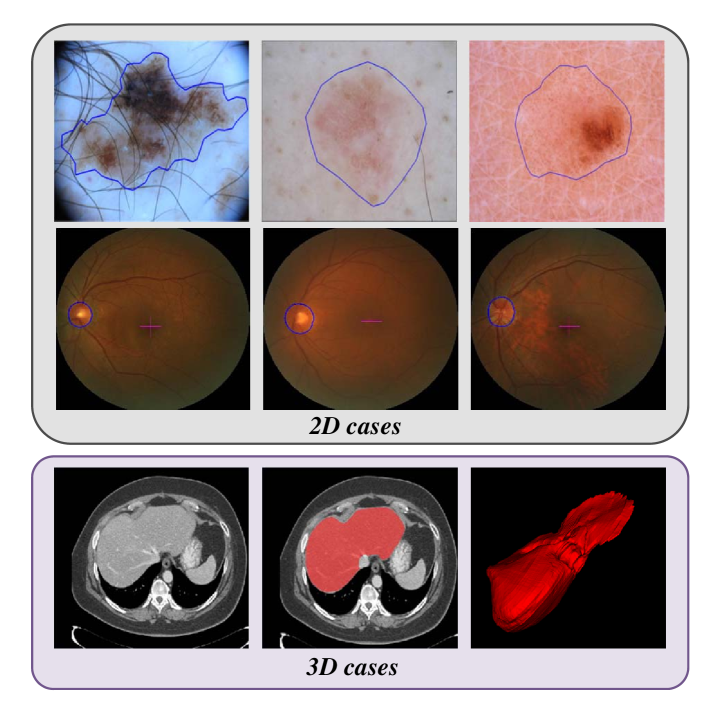
Figure 1: Three common medical image segmentation tasks. The first, second, and third rows show the skin lesion in the dermoscopy image, the optical disc in retinal fundus images, and liver segmentations from CT scans. Blue color denotes the structure boundary and red color represents the liver.

Segmenting anatomical structural or abnormal regions from medical images, such as dermoscopy images, fundus images, and 3D computed tomography (CT) scans, is of great significance for clinical practice, especially for disease diagnosis and treatment planning. Recently, deep learning techniques have made impressive progress on semantic image segmentation tasks and become a popular choice in both computer vision and medical imaging community [1, 2]. The success of deep neural networks usually relies on the massive labeled dataset. However, it is hard and expensive to obtain labeled data, notably in the medical imaging domain where only experts can provide reliable annotations [3]. For example, there are thousands of dermoscopy image records in the clinical center, but melanoma delineation by experienced dermatologists is very scarce; see Figure 1. Such cases can also be observed in the optic disc segmentation from the retinal fundus images, and especially in liver segmentation from CT scans, where delineating organs from volumetric images in a slice-by-slice manner is very time-consuming and expensive. The lack of the labeled data motivates the study of methods that can be trained with limited supervision, such as semi-supervised learning [4, 5, 6], weakly supervised learning [7, 8, 9], and unsupervised domain adaptation [10, 11, 12], etc. In this paper, we focus on the semi-supervised segmentation approaches, considering that it is relatively easy to acquire a large amount of unlabeled medical image data.

Semi-supervised learning aims to learn from a limited amount of labeled data and an arbitrary amount of unlabeled data, which is a fundamental, challenging problem and has a high impact on real-world clinical applications. The semi-supervised problem has been widely studied in medical image research community [13, 14, 15, 16, 17]. Recent progress in semi-supervised learning for medical image segmentation has featured deep learning [18, 5, 19, 20, 21]. Bai et al. [18] present a semi-supervised deep learning model for cardiac MR image segmentation, where the segmented label maps from unlabeled data are incrementally added into the training set to refine the segmentation network. Other semi-supervised learning methods are based on the recent techniques, such as variational autoencoder (VAE) [5] and generative adversarial network (GAN) [19]. We tackle the semi-supervised segmentation problem from a different point of view. With the success of the self-ensembling model in the semi-supervised classification problem [22], we further advance the method to medical image segmentation tasks, including 2D cases and 3D cases.

In this paper, we present a new semi-supervised learning method based on the self-ensembling strategy for medical image segmentation. The whole framework is trained with a weighted combination of supervised and unsupervised losses. The supervised loss is designed to utilize the labeled data for accurate predictions. To leverage the unlabeled data, our self-ensembling method encourages a consistent prediction of the network for the same input under different regularizations, e.g., randomized Gaussian noise, network dropout, and randomized data transformation. In particular, our method accounts for the challenging segmentation task, in which pixel-level classification is required to be predicted. We observe that in the segmentation problem, if one transforms (e.g., rotates) the input image, the expected prediction should be transformed in the same manner. When the inputs of CNNs are rotated, the corresponding network predictions would not rotate in the same way [23]. In this regard, we take advantage of this property by introducing a transformation (i.e., rotation, flipping) consistent scheme at the input and output space of our network. Specifically, we design the unsupervised loss by minimizing the differences between the network predictions under different transformations of the same input. To further improve the regularization, we extend the transformation consistency regularization with the scaling operation and optimize the network under a scaling consistent scheme. Also, we adopt a teacher model to evaluate images under perturbations to construct better targets. We extensively evaluate our methods for semi-supervised medical image segmentation on three representative segmentation tasks, i.e., skin lesion segmentation from dermoscopy images, optic disc segmentation from retinal images, and liver segmentation from CT scans. In summary, our semi-supervised method achieves significant improvements compared with the supervised baseline and also outperforms other semi-supervised segmentation methods.

The main contributions of this paper are:

• We present a novel and effective semi-supervised method, namely TCSM_v2, for medical image segmentation. Our method is flexible and can be easily applied to both 2D and 3D convolutional neural networks.

• We regularize unlabeled data with the transformation-consistent strategy and demonstrate effective semi-supervised medical image segmentation.

• Extensive experiments on three representative yet challenging medical image segmentation tasks, including 2D and 3D datasets, demonstrate the effectiveness of our semi-supervised method over other methods.

• Our method excels other state-of-the-art methods and establishes a new record in the ISIC 2017 skin lesion segmentation dataset with the semi-supervised method.

This work extends our previous work TCSM [24] in three aspects. First, multi-scale inference is an effective technique utilized in many image recognition tasks [25, 26, 27]. To enhance the regularization, we extend TCSM with more generalized transformation, such as random scaling. Through this, we utilize the unlabeled data to improve the regularization of the network. Second, our preliminary TCSM evaluates the inputs with perturbations on the same network. To avoid the misrecognition, we incorporate a teacher model to construct better targets, where the teacher model is an exponential moving average of the student model. Thirdly, we evaluate our method on three datasets, including the skin lesion dataset, retinal fundus dataset, and liver CT dataset. Experiments on all three datasets show the effectiveness of our method over existing methods for semi-supervised medical image segmentation.

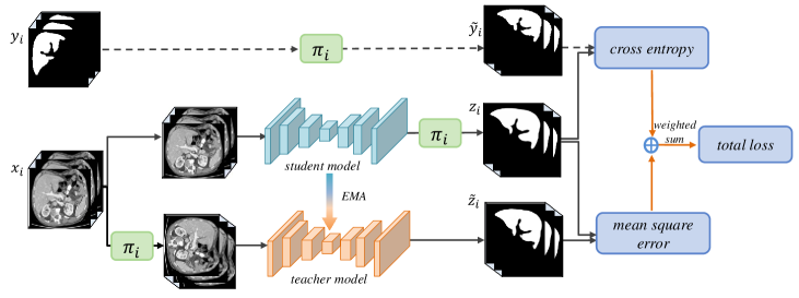
Figure 2: Our transformation-consistent self-ensembling model (TCSM_v2) for semi-supervised medical image segmentation (we use liver CT scans as example). The teacher and student models share the same architecture, and the weight of the teacher model is the exponential moving average (EMA) of the student model. The student model is trained by the total loss, which is a weighted combination of the cross-entropy loss on labeled data, and mean square error loss on both labeled and unlabeled data. The model encourages the teacher and student models to be transformation-consistent by utilizing the unlabeled data. $\pi_{i}$ refers to the transformation-consistent regularization, including rotation, flipping, and scaling operations.

II Related Work

Semi-supervised segmentation for medical images. Early semi-supervised works segment medical images mainly using hand-crafted features [13, 14, 15, 16, 17]. You et al. [13] combined radial projection and self-training learning to improve the segmentation of retinal vessel from fundus image. Portela et al. [14] presented a clustering-based Gaussian mixture model to automatically segment brain MR images. Later on, Gu et al. [16] constructed forest oriented superpixels for vessel segmentation. For skin lesion segmentation, Jaisakthi et al. [17] explored K-means clustering and flood fill algorithm. These semi-supervised methods are, however, based on hand-crafted features, which suffer from limited representation capacity.

Recent works for semi-supervised segmentation are mainly based on deep learning. An iterative method is proposed by Bai et al. [18] for cardiac segmentation from MR images, where network parameters and segmentation masks for unlabeled data are alternatively updated. Generative model based semi-supervised approaches are also popular in the medical image analysis community [5, 19, 28, 29]. Sedai et al. [5] introduced a variational autoencoder (VAE) for optic cup segmentation from retinal fundus images. They learned the feature embedding from unlabeled images using VAE, and then combined the feature embedding with the segmentation autoencoder trained on the labeled images for pixel-wise segmentation of the cup region. To involve unlabeled data in training, Nie et al. [19] presented an attention-based GAN approach to select trustworthy regions of the unlabeled data to train the segmentation network. Another GAN-based work [29] employed the cycle-consistency principle and performed experiments on cardiac MR image segmentation. More recently, Ganaye et al. [21] proposed a semi-supervised method for brain structures segmentation by taking advantage of the invariant nature and semantic constraint of anatomical structures. Multi-view co-training based methods [4, 30] have also been explored on 3D medical data. Differently, our method takes the advantage of transformation consistency and self-ensembling model, which is simple yet effective for medical image segmentation tasks.

Transformation equivariant representation. Next, we review equivariance representations, to which the transformation equivariance is encoded in the network to explore the network equivariance property [31, 32, 23, 33]. Cohen and Welling [31] proposed a group equivariant neural network to improve the network generalization, where equivariance to $90\mathrm{°}$-rotations and dihedral flips are encoded by copying the transformed filters at different rotation-flip combinations. Concurrently, Dieleman et al. [32] designed four different equivariance to preserve feature map transformations by rotating the feature maps instead of the filters. Recently, Worrall et al. [23] restricted the filters to circular harmonics to achieve continuous $360\mathrm{°}$-rotations equivariance. However, these works aim to encode equivariance into the network to improve its generalization capability, while our method aims to better utilize the unlabeled data in semi-supervised learning.

Medical image segmentation. Early methods for medical image segmentation mainly focused on using thresholding [34], statistical shape models [35] and machine learning [36, 37, 38, 39, 40], while recent ones are mainly deep-learning-based [41, 42, 43]. Deep learning methods showed promising results on skin lesion segmentation, optic disc segmentation, and liver segmentation [44, 45, 46, 47, 48]. Yu et al. [44] explored the network depth property and developed a deep residual network for automatic skin lesion segmentation by stacking residual blocks to increase the network’s representative capability. Yuan et al. [49] trained a 19-layer deep convolutional neural network in an end-to-end manner for skin lesion segmentation. As for optical disc segmentation, Fu et al. [45] presented an M-Net for joint OC and OD segmentation. Also, a disc-aware network [45] was designed for glaucoma screening by an ensemble of different feature streams of the network. For liver segmentation, Chlebus et al. [40] presented a cascaded FCN combined with hand-crafted features. Li et al. [50] presented a 2D-3D hybrid architecture for liver and tumor segmentation from CT images. Although these methods achieved good results, they are based on fully supervised learning, requiring massive pixel-wise annotations from experienced dermatologists or radiologists.

III Method

Figure 2 overviews our transformation-consistent self-ensembling model (TCSM_v2) for semi-supervised medical image segmentation. First, we randomly sample $x_{i}$ raw data, including both the labeled and unlabeled cases from the training dataset, followed by performing random transformations on these images. Teacher and student models are formulated in our framework, where the student model is trained by the loss function and the teacher model is an average of consecutive student models. To train the student model, the transformed inputs are fed into the student model and the softmax output is compared with a one-hot label using classification cost (cross-entropy in Figure 2) and with the teacher output using consistency cost (mean square error in Figure 2). After the weights of the student model have been updated with gradient descent, the teacher model weights are updated as an exponential moving average of the student weights. Hence, the label information is passed to the unlabeled data by constraining the model outputs to be consistent with the unlabeled data.

III-A Mean Teacher Based Semi-supervised Framework

To ease the description of our method, we first formulate the semi-supervised segmentation task. In the semi-supervised segmentation problem, the training set consists of $N$ inputs in total, including $M$ labeled inputs and $N-M$ unlabeled inputs. We denote the labeled set as $\mathcal{L}=\left\{(x_{i},y_{i})\right\}_{i=1}^{M}$ and the unlabeled set as $\mathcal{U}=\left\{x_{i}\right\}_{i=M+1}^{N}$. For the 2D images, $x_{i}\in\mathbb{R}^{H\times W\times 3}$ denotes the input image and $y_{i}\in\{0,1\}^{H\times W}$ is the ground-truth segmentation mask. For the 3D volumes, $x_{i}\in\mathbb{R}^{H\times W\times D}$ denotes the input volume and $y_{i}\in\{0,1\}^{H\times W\times D}$ is the ground-truth segmentation volume. The general semi-supervised segmentation learning tasks can be formulated to learn the network parameters $\theta$ by optimizing:

$$\min_{\theta}\sum_{i=1}^{M}l(f(x_{i};\theta),y_{i})+\lambda R(\theta,\mathcal{L},\mathcal{U}),$$ (1)

where $l$ is the supervised loss function, $R$ is the regularization (unsupervised) loss, and $f(\cdot)$ is the segmentation neural network and $\theta$ denotes the model weights. $\lambda$ is a weighting factor that controls how strong the regularization is. The first term in the loss function is trained by the cross-entropy loss, aiming at evaluating the correctness of network output on labeled inputs only. The second term is optimized with the regularization loss, which utilizes both the labeled and unlabeled inputs.

The key point of this semi-supervised learning is based on the smoothness assumption, i.e., data points close to each other in the image space are likely to be close in the label space [51, 22]. Specifically, these methods focus on improving the target quality using self-ensembling and exploring different perturbations, which include the input noise and the network dropout. The network with the regularization loss encourages the predictions to be consistent and is expected to give better predictions. The regularization loss $R$ can be described as:

$$R(\theta,\mathcal{L},\mathcal{U})=\sum_{i=1}^{N}\mathbb{E}_{\xi^{{}^{\prime}},\xi}\left\|f(x_{i};\theta,\xi^{{}^{\prime}})-f(x_{i};\theta,\xi)\right\|^{2},$$ (2)

where $\xi$ and $\xi^{\prime}$ denote to different regularization and perturbations of input data, respectively. In our work, we share the same spirit as these methods by designing different perturbations for the input data. Specifically, we design the regularization term as a consistency loss to encourage smooth predictions for the same data under different regularization and perturbations (e.g., Gaussian noise, network dropout, and randomized data transformation).

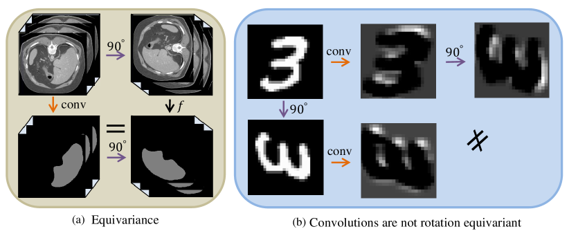
Figure 3: (a) Segmentation is desired to be rotation equivariant. If the input image is rotated, the ground truth mask should be rotated in the same manner. (b) Convolutions are not rotation equivariant in general. If the input image is rotated, the generated output is not the same with the original output that rotated in the same manner.

In the above, we evaluate the model twice to get two predictions under different perturbations. In this case, the model assumes a dual role as a teacher and as a student. As a student, it learns as before, while as a teacher, it generates targets, which are then used by itself as a student for learning. The model generates the targets by itself, thus it may be incorrect, especially when excessive weight is given to the generated targets. To construct better targets, we employ the mean teacher based framework [52], where the teacher model $f_{{\theta}^{{}^{\prime}}}$ uses the exponential moving average (EMA) weights of the student model $f_{{\theta}}$, i.e., $\theta^{{}^{\prime}}_{t}=\alpha\theta^{{}^{\prime}}_{t-1}+(1-\alpha)\theta_{t}$. Specifically, the weight of teacher model $\theta_{t}^{{}^{\prime}}$ is updated through $\theta_{t}^{{}^{\prime}}=\alpha\theta^{{}^{\prime}}_{t-1}+(1-\alpha)\theta_{t}$, where $\theta_{t}$ is the student model parameters and $\theta_{t}^{{}^{\prime}}$ is the teacher model parameters. $\alpha$ is a smoothing coefficient hyperparameter that affects how the teacher model relies on the current student model parameter. If $\alpha$ is large, the teacher model relies more on the previous teacher model in the last step; otherwise, the teacher model relies more on the current student model parameters. According to the empirical evidence in [52], setting $\alpha$ = 0 makes the model as a variation of the $\pi$ model, and the performance is the best when setting $\alpha$ = 0.999. We follow this empirical experience and set $\alpha$ to 0.999 in our experiments. Then, the transformation-consistent regularization is performed on the input to the teacher model $f_{{\theta}^{{}^{\prime}}}$, and the consistency loss is added on the two predictions of the teacher and student model, respectively.

III-B Transformation Consistent Self-ensembling Model

Next, we introduce how we design the randomized data transformation regularization for segmentation, i.e., the transformation-consistent self-ensembling model (TCSM_v2).

III-B1 Motivation

In general self-ensembling semi-supervised learning, most regularization and perturbations can be easily designed for the classification problem. However, in the medical image domain, accurate segmentation of important structures or lesions is a very challenging problem and the perturbations for segmentation tasks are more worthy to explore. One prominent difference between these two common tasks is that the classification problem is transformation invariant while the segmentation task is expected to be transformation equivariant. Specifically, for image classification, the convolutional neural network only recognizes the presence or absence of an object in the whole image. In other words, the classification result should remain the same, no matter what the data transformation (i.e., translation, rotation, and flipping) are applied to the input image. While in the image segmentation task, if the input image is rotated, the segmentation mask is expected to have the same rotation with the original mask, although the corresponding pixel-wise predictions are the same; see examples in Figure 3 (a). However, in general, convolutions are not transformation (i.e., flipping, rotation) equivariant, meaning that if one rotates or flips the CNN input, then the feature maps do not necessarily rotate in a meaningful manner [23], as shown in Figure 3 (b). Therefore, the convolutional network consisting of a series of convolutions is also not transformation equivariant. Formally, every transformation $\pi\in\Pi$ of input x associates with a transformation $\psi\in\Psi$ of the outputs; that is $\psi[f(\textbf{x})]=f(\pi[\textbf{x}]),$ but in general $\pi\neq\psi$.

III-B2 Mechanism of TCSM

This phenomenon limits the unsupervised regularization effect of randomized data transformation for segmentation [22]. To enhance the regularization and more effectively utilize unlabeled data in our segmentation task, we introduce a transformation-consistent scheme in the unsupervised regularization term. Specifically, this transformation-consistent scheme is embedded in the framework by approximating $\psi$ to $\pi$ at the input and output space. Figure 2 shows the detailed illustration of the framework and Algorithm 1 shows the pseudocode. Under the transformation-consistent scheme and other different perturbations (e.g., Gaussian noise and network dropout), each input $x_{i}$ is fed into the network for twice evaluation to acquire two outputs $z_{i}$ and $\tilde{z}_{i}$. More specifically, the transformation-consistent scheme consists of triple $\pi_{i}$ operations; see Figure 2. For one training input $x_{i}$, in the first evaluation, the operation $\pi_{i}$ is applied to the input image while in the second evaluation, the operation $\pi_{i}$ is applied to the prediction map. Random perturbations (e.g., Gaussian noise and network dropout) are applied in the network during the twice evaluations. By minimizing the difference between $z_{i}$ and $\tilde{z}_{i}$ with a mean square error loss, the network is regularized to be transformation-consistent and thus increase the network generalization capacity. Notably, the regularization loss is evaluated on both the labeled and unlabeled inputs. To utilize the labeled data $x_{i}\in\mathcal{L}$, the same operation $\pi_{i}$ is also performed on $y_{i}$ and optimized by the standard cross-entropy loss. Finally, the network is trained by minimizing a weighted combination of unsupervised regularization loss and supervised cross-entropy loss.

Algorithm 1 TCSM_v2 Algorithm pseudocode.

1:$x_{i}\in{\mathcal{L}+\mathcal{U}},y_{i}\in\mathcal{L}$

2:$\lambda(T)$ = unsupervised weight function

3:$f_{\theta}(x)$ = student model with parameters $\theta$

4:$f_{\theta^{{}^{\prime}}}(x)$ = teacher model with parameters $\theta^{{}^{\prime}}$

5:$\pi_{i}(x)$ = transformation operations

6:$\alpha$ = smoothing coefficient hyperparameter.

7:for $T$ in $[1,numepochs]$ do

8:     for each minibatch $B$ do

9:         randomly update $\pi_{i}(x)$

10:         $z_{i\in B}$ $\leftarrow\pi_{i}(f_{\theta}(x_{i\in B}))$

11:         $\tilde{z}_{i\in B}\leftarrow f_{\theta^{{}^{\prime}}}(\pi_{i}(x_{i\in B}))$

12:         $loss\leftarrow-\frac{1}{\left|B^{{}^{\prime}}\right|}\sum_{i\in(B^{{}^{\prime}})}{\rm log}z_{i}[\pi_{i}(y_{i})]+$

13:         $\lambda(T)\frac{1}{\left|B\right|}\sum_{i\in B}\left\|z_{i}-\tilde{z}_{i}\right\|^{2}$

14:         update $\theta$ using optimizer

15:         update $\theta^{{}^{\prime}}_{T}\leftarrow\alpha\theta^{{}^{\prime}}_{T-1}+(1-\alpha)\theta_{T}$

16:     end for

17:end for

18:return $\theta^{{}^{\prime}}$;

III-B3 Loss function

It has cross-entropy loss on the labeled inputs and the regularization term on both the labeled and unlabeled inputs. The overall loss function is then defined as

$$loss=\mathcal{L}+\lambda(T)\mathcal{R},\vspace*{-0.5mm}$$ (3)

where $\mathcal{L}$ and $\mathcal{R}$ are the supervised term and regularization term, respectively. The time-dependent warming up function $\lambda(T)$ is a weighting factor for supervised loss and regularization loss. This weighting function is a Gaussian ramp-up curve, i.e., $\lambda(T)=k*e^{(-5(1-T)^{2})}$, where $T$ denotes the training epoch and $k$ scales the maximum value of the weighting function. In our experiments, we empirically set $k$ as 1.0.

We randomly sample $x_{i\in B}$ images from the training data and the supervised term $\mathcal{L}$ within one minibatch is defined as

$$\vspace*{-2.5mm}\mathcal{L}=-\frac{1}{\left|B^{{}^{\prime}}\right|}\sum_{i\in B^{{}^{\prime}}}{\rm log}z_{i}[\pi_{i}(y_{i})],\vspace*{-0.3mm}$$ (4)

where $B^{{}^{\prime}}\in B$ denotes the labeled images within a minibatch, $z_{i}$ and $y_{i}$ are the network prediction and ground-truth segmentation label, respectively. At the beginning of the network training, $\lambda(T)$ is small and training is mainly dominated by the supervised loss on the labeled data. In this way, the network is able to learn accurate information from the labeled data. As the training progresses, the network gets a reliable model and can generate output for the unlabeled data. The regularization term optimizes the prediction differences by calculating the differences on the predictions.

$$\mathcal{R}=\frac{1}{\left|B\right|}\sum_{i\in B}\left\|z_{i}-\tilde{z}_{i}\right\|^{2},$$ (5)

where $z_{i}$ and $\tilde{z}_{i}$ denote the network predictions of the student model and teacher model, respectively, i.e., $z_{i}=\pi_{i}(f_{\theta}(x_{i\in B}))$ and $\tilde{z}_{i}=f_{\theta^{{}^{\prime}}}(\pi_{i}(x_{i\in B}))$. $f_{\theta}$ and $f_{\theta^{{}^{\prime}}}$ denote the student model and teacher model, respectively. The student model $f_{\theta}$ is updated by the gradient descent while the teacher model is updated by ${\theta^{{}^{\prime}}_{T}}=\alpha{\theta^{{}^{\prime}}_{T-1}}+(1-\alpha)\theta_{T}$, where $\alpha=0.999$.

III-B4 Implementation of $\pi$ operation

Multi-scale ensembling is shown to be effective for image recognition [25, 27, 26]. To enlarge the regularization effect for semi-supervised learning, we extend the TCSM to a more generalized form including random scaling. The main goal is to keep the consistency of the teacher and student model after multi-scale inference. Specifically, $\pi_{i}$ operation includes not only rotation but also random scaling operation. For the student model, we give the input and generate the prediction $z_{i}$. For the teacher model, we randomly scale the input image and generate the prediction result, which is then rescaled to the original size of the input image and we finally get $\tilde{z_{i}}$. Then, two predictions $z_{i}$ and $\tilde{z_{i}}$ are minimized through a mean square error loss.

The transformation-consistent scheme includes random scaling, the horizontal flipping operation as well as four kinds of rotation operations to the input with angles of $\gamma\cdot 90^{\circ},$ where $\gamma\in\left\{0,1,2,3\right\}$. During each training pass, one rotation operation and one scaling operation within the scaling ratio of 0.8-1.2 is randomly chosen and applied to the input image, i.e., $\pi_{i}(x_{i})$. To keep two terms in the loss function, we evenly and randomly select the labeled and the unlabeled samples in each minibatch. Note that we employed the same data augmentation in the training procedure of all the experiments for a fair comparison. However, our method is different from traditional data augmentation. Specifically, our method utilized the unlabeled data by minimizing the network output difference under the transformed inputs, while complying with the smoothness assumption.

III-C Technical Details of TCSM_v2

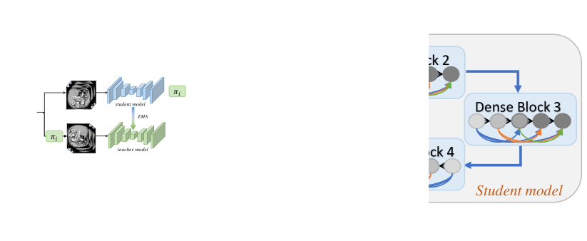
Figure 4: The visualization of transformation-consistent operation $\pi$ in the DenseUnet architecture. We omit the unet connection and the decoder part for simplification.

For dermoscopy images and retinal fundus images, we employ the 2D DenseUNet architecture [50] as both our teacher and student models. Compared to the standard DenseNet [53], we add the decoder part for the segmentation tasks. The decoder has four blocks and each block consists of "upsampling, convolutional, batch normalization and ReLU activation" layers. The UNet-like skip connection is added between the final convolution layer of each dense block in the encoder part and the convolution layer in the decoder part. The final prediction layer is a convolutional layer with a channel number of two. Before the final convolution layer, we add a dropout layer with a drop rate of 0.3. The network was trained with Adam algorithm [54] with a learning rate of 0.0001. All the experiments are trained for a total of 8000 iterations. We also visualize the network structure diagram to illustrate the implementation of TCSM in Figure 4.

To generalize our method to 3D medical images, e.g., liver CT scans, we train TCSM_v2 with 3D U-Net [41]. For training with 3D U-Net, we follow the original setting with the following modifications. We modify the base filter parameters to 32 to accommodate this input size. The optimizer is SGD with a learning rate of 0.01. The batch normalization layer is employed to facilitate the training process and the loss function is modified to the standard weighted cross-entropy loss. All the experiments are trained for a total of 9000 iterations.

We implemented the model using PyTorch [55]. The experiments differ slightly from that in [24] due to the different implementation platforms. We used the standard data augmentation techniques on-the-fly to avoid overfitting, including randomly flipping, rotating, and scaling with a random scale factor from 0.9 to 1.1. Note that all the experiments employed data augmentation for a fair comparison. In the inference phase, we remove the transformation operations in the network and do one single test with the original input for a fair comparison. After getting the probability map from the network, we first apply thresholding with 0.5 to generate the binary segmentation result, and then use morphology operation, i.e., filling holes, to obtain the final segmentation result.

IV Experiments

IV-A Datasets

To evaluate our method, we conduct experiments on various modalities of medical images, including dermoscopy images, retinal fundus images, and liver CT scans.

Dermoscopy image dataset. The dermoscopy image dataset in our experiments is the 2017 ISIC skin lesion segmentation challenge dataset [56]. It includes a training set with 2000 annotated dermoscopic images, a validation set with 150 images, and a testing set with 600 images. The image size ranges from $540\times 722$ to $4499\times 6748$. To balance the segmentation performance and computational cost, we first resize all the images to $248\times 248$ using bicubic interpolation.

Retinal fundus image dataset. The fundus image dataset is from the MICCAI 2018 Retinal Fundus Glaucoma Challenge (REFUGE). Manual pixel-wise annotations of the optic disc were obtained by seven independent ophthalmologists from the Zhongshan Ophthalmic Center, Sun Yat-sen University. Experiments were conducted on the released training dataset, which contains 400 retinal images. The training dataset is randomly split to training and test sets, and we resize all the images to $248\times 248$ using bicubic interpolation.

Liver segmentation dataset. The liver segmentation dataset are from the 2017 Liver Tumor Segmentation Challenge (LiTS) [57, 58]. The LiTS dataset contains 131 and 70 contrast-enhanced 3D abdominal CT scans for training and testing, respectively. The dataset was acquired by different scanners and protocols at six different clinical sites, with a largely varying in-plane resolution from 0.55 mm to 1.0 mm and slice spacing from 0.45 mm to 6.0 mm.

IV-B Evaluation Metrics

For dermoscopy image dataset, we use Jaccard index (JA), dice coefficient (DI), pixel-wise accuracy (AC), sensitivity (SE) and specificity (SP) to measure the segmentation performance:

$$AC=\frac{TP+TN}{TP+FP+TN+FN},$$

$$SE=\frac{TP}{TP+FN},\quad SP=\frac{TN}{TN+FP},$$ (6)

$$JA=\frac{TP}{TP+FN+FP},\quad DI=\frac{2\cdot TP}{2\cdot TP+FN+FP},$$

where $TP,TN,FP$, and $FN$ refer to the number of true positives, true negatives, false positives, and false negatives, respectively. For the retinal fundus image dataset, we use JA to measure the optic disc segmentation accuracy. For the liver CT dataset, Dice per case score is employed to measure the accuracy of the liver segmentation result, according to the evaluation of the 2017 LiTS challenge [57].

IV-C Experiments on Dermoscopy Image Dataset

Table I: Comparison of supervised learning and semi-supervised learning (50 labeled/1950 unlabeled) on the validation set in the dermoscopy image dataset. "Supervised+reg" denotes supervised with regularization.

Metric	Supervised	Supervised+regu	Ours
JA	71.17	72.28	75.24
DI	79.91	81.10	83.44
AC	91.95	93.52	94.46
SE	75.90	81.17	83.07
SP	97.04	97.02	97.07

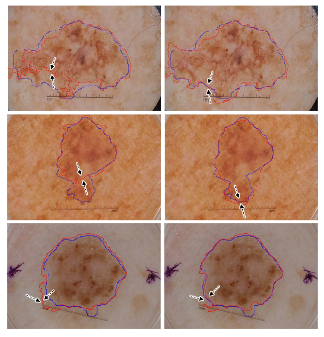
Figure 5: Examples of the segmentation results of supervised learning (left) and our method (right) on the validation set in the dermoscopy image dataset. The blue and red contours denote the ground truth and our segmentation result, respectively.

IV-C1 Quantitative and visual results with 50 labeled data

We report the performance of our method trained with only 50 labeled images and 1950 unlabeled images. Note that the labeled image is randomly selected from the whole dataset. Table I shows the experiments with the supervised method, supervised with regularization, and our semi-supervised method on the validation dataset. We use the same network architecture (DenseUNet) in all these experiments for a fair comparison. The supervised experiment is optimized by the standard cross-entropy loss on the 50 labeled images. The supervised with regularization experiment is also trained with 50 labeled images, but differently, the total loss function is a weighted combination of the cross-entropy loss and the regularization loss, which is the same with our loss function. Our method is trained with 50 labeled and 1950 unlabeled images in a semi-supervised manner. From Table I, it is observed that our semi-supervised method achieves higher performance than a supervised counterpart on all the evaluation metrics, with prominent improvements of 4.07% on JA and 3.47% on DI, respectively. It is worth mentioning that supervised with regularization experiment improves the supervised training due to the regularization loss on the labeled images; see "Supervised+regu" in Table I. The consistent improvements of "Supervised+regu" on all evaluation metrics demonstrate the regularization loss is also effective for the labeled images. Figure 5 presents some segmentation results (red contour) of supervised method (left) and our method (right). Comparing with the segmentation contour achieved by the supervised method (left column), the semi-supervised method fits more consistently with the ground-truth boundary. The observation shows the effectiveness of our semi-supervised learning method, compared with the supervised method.

Table II: Ablation of semi-supervised method (50 labeled/1950 unlabeled) on the validation set in dermoscopy image dataset. “R” denotes rotation transformation. “ND” denotes Gaussian noise and dropout. “NDR” denotes Gaussian noise, dropout, and rotation. “Shift ($r$)” denotes shifting transformation with ratio $r$. “NDRscale” denotes the transformations including noise, dropout, rotation, and random scaling. (Unit: %).

Setting	JA	DI	AC	SE	SP
Supervised	71.17	79.91	91.95	75.90	97.04
TCSM-R	73.76	82.05	94.87	84.14	97.65
TCSM-ND	74.03	82.33	94.30	83.84	96.77
TCSM-NDR	74.46	82.22	95.06	82.51	97.42
TCSM_v2-NDR	74.91	82.90	94.63	82.80	97.61
TCSM_v2-Shift(0.3)	71.26	75.11	79.5	78.32	85.40
TCSM_v2-Shift(0.2)	71.69	79.24	92.34	80.12	95.42
TCSM_v2-Shift(0.1)	72.74	80.93	93.35	81.32	96.62
TCSM_v2-Scale(0.3)	71.62	79.96	92.69	79.86	97.76
TCSM_v2-Scale(0.2)	71.87	79.78	92.75	79.98	96.04
TCSM_v2-Scale(0.1)	73.57	81.51	94.24	80.57	96.90
TCSM_v2-NDRScale(ours)	75.24	83.44	94.46	83.07	97.07

IV-C2 Effectiveness of TCSM and TCSM_v2

To show the effectiveness of our proposed transformation-consistent method, we conducted an ablation analysis of our method on the dermoscopy image dataset, as the results are shown in Table II. The experiments were performed with randomly-selected 50 labeled data and 1950 unlabeled data, and tested on the validation set. In the “Supervised” setting, we trained the network with only 50 labeled data. “TCSM-ND” refers to semi-supervised learning with Gaussian noise and dropout regularization. “TCSM-R” refers to semi-supervised learning with transformation-consistent regularization (only rotation), and “TCSM” refers to the experiment with all of these regularizations. As shown in Table II, both kinds of regularizations independently contribute to the performance gains of semi-supervised learning. The resulting improvement with transformation-consistent regularization is very competitive, compared with the performance increment with Gaussian noise and dropout regularizations. These two regularizations are complementary, so when they are employed together, the performance can be further enhanced.

Moreover, we analyze the effects of the shifting and scaling operations. Shift ($r$) denotes randomly shifting the image by $r^{\prime}W$ or $r^{\prime}H$, where $r^{\prime}\in[1-r,1+r]$, and $W$ and $H$ denote the image width and height. Scale ($r$) denotes randomly scaling the image to $(r^{\prime}W,r^{\prime}H)$, where $r^{\prime}\in[1-r,1+r]$. From the experiments in Table II, we can see that random scaling with ratio 0.1 could improve the semi-supervised learning results, while other transformation settings have limited improvements. “TCSM_v2-NDR” denotes the mean teacher based semi-supervised learning with transformation-consistent strategy (only rotation). “TCSM_v2-NDRScale” refers to the mean teacher based semi-supervised learning with our transformation-consistent strategy including both rotation and scaling. From these two comparisons, we can see that the generalized form of transformation-consistent strategy improves the semi-supervised learning. “TCSM” and “TCSM_v2-NDR” utilizes the same regularization. From these two comparisons, we can find that the weight-averaged consistency targets improve the semi-supervised deep learning results. Our final model achieves 75.24% JA and 83.44% DI, surpassing the supervised baseline by 5.7% JA and 4.4% DI.

IV-C3 Results under different number of labeled data

Table III: Results of our method on the validation set under different number of labeled/unlabeled images (Unit:%).

Label/Unlabel	Metric	Supervised	TCSM	TCSM_v2
50/1950	JA	71.17	74.46	75.24
	DI	79.91	82.22	83.44
	AC	91.95	95.06	94.46
	SE	75.90	82.51	83.07
	SP	97.04	97.42	97.07
100/1900	JA	73.92	74.75	75.52
	DI	82.37	83.02	83.35
	AC	93.87	94.03	93.28
	SE	83.95	86.02	83.78
	SP	97.08	96.89	94.65
300/1700	JA	76.66	77.19	77.52
	DI	84.32	85.38	85.20
	AC	94.25	95.11	95.90
	SE	85.82	86.02	86.31
	SP	95.77	95.78	95.85
2000/0	JA	78.80	79.15	79.27
	DI	86.67	87.01	88.13
	AC	95.12	95.03	96.01
	SE	88.75	89.20	89.35
	SP	97.02	96.91	97.14

Table III shows the lesion segmentation results of our TCSM and TCSM_v2 (trained with labeled data and unlabeled data) and supervised method (trained only with labeled data) under a different number of labeled/unlabeled images. We draw the JA score of the results in Figure 6. It is observed that the semi-supervised methods consistently performs better than the supervised method in different labeled/unlabeled data settings, demonstrating that our method effectively utilizes the unlabeled data and brings performance gains. Note that in all semi-supervised learning experiments, we train the network with 2000 images in total, including labeled images and unlabeled images. As expected, the performance of supervised training increases when more labeled training images are available; see the blue line in Figure 6. At the same time, the segmentation performance of semi-supervised learning can also increase with more labeled training images; see the orange line in Figure 6. The performance gap between supervised training and semi-supervised learning narrows as more labeled samples are available, which conforms with our expectations. When the amount of labeled dataset is small, our method can gain a large improvement, since the regularization loss can effectively leverage more information from the unlabeled data. Comparatively, as the number of labeled data increases, the improvement becomes limited. This is because the labeled and unlabeled data are randomly selected from the same dataset and a large amount of labeled data may reach the upper bound performance of the dataset.

From the comparison between TCSM and TCSM_v2, we can see that TCSM_v2 consistently improve TCSM under different label and unlabeled settings. From the comparison between the semi-supervised method and supervised method trained with 2000 labeled images in Figure 6, it can be observed that our method increases the JA performance when all labels are used. The improvement indicates that the unsupervised loss can also provide a regularization to the labeled data. In other words, the consistency requirement in the regularization term can encourage the network to learn more robust features to improve the segmentation performance.

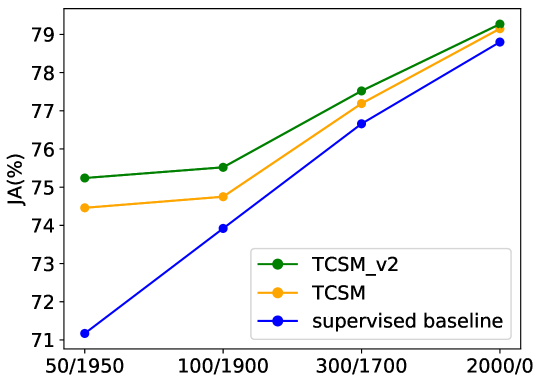
Figure 6: Results on the validation set of the dermoscopy image dataset with different number of labeled/unlabeled data.

IV-C4 Comparison with other semi-supervised segmentation methods

We compare our method with two latest semi-supervised segmentation methods [18, 28] in the medical imaging community and an adversarial learning-based semi-supervised method [59]. Also, we extend the semi-supervised classification model [52] to segmentation for comparison. Note that the method [19] for medical image segmentation adopts a similar idea with the adversarial learning-based method [59].

Table IV: JA performance of different semi-supervised methods on the validation dataset of the dermoscopy image dataset. “Supervised” denotes training with 50 labeled data (Unit: %).

Method	Backbone	Result	Improvement
Supervised	DenseUNet	71.17	-
GAN [59]		73.31	2.14
DAN [28]		73.82	2.65
Mean Teacher [52]		74.23	3.06
Self-training [18]		74.40	3.23
Ours		75.24	4.07

For a fair comparison, we re-implemented their methods with the same network backbone on this dataset. All the experiments utilized the same data augmentation and training strategies. We conducted experiments with the setting of 50 labeled images and 1950 unlabeled images. Table IV shows the JA performance of different methods on the validation set. As shown in Table IV, our method achieves 4.07% JA improvement by utilizing unlabeled data. Compared with other methods, we achieve the highest improvement over the supervised baseline. The comparison shows the effectiveness of our semi-supervised segmentation method, compared to other semi-supervised methods.

IV-C5 Comparison with methods on the challenge leaderboard

We also compare our method with state-of-the-art methods submitted to the ISIC 2017 skin lesion segmentation challenge [56]. There are a total of 21 submissions and the top results are listed in Table V. Note that the final rank is determined according to JA on the testing set. We trained two models: TCSM_v2 and baseline. TCSM_v2 was trained with 300 labeled images and the left are utilized as the unlabeled images. The baseline model is trained with only 300 labeled data. Other methods use all labeled data as the training data. The supervised model is denoted as our baseline model. As shown in Table V, our semi-supervised method achieved the best performance on the benchmark, outperforming the state-of-the-art method [60] with 1.6% improvement on JA (from 76.5% to 78.1%). The performance gains on DI and SE are consistent with that on JA, with 1.1% and 3.7% improvement, respectively. Our baseline model with 300 labeled data also outperforms other methods due to state-of-the-art network architecture. Based on this strong baseline, our semi-supervised learning method further makes significant improvements, which demonstrates the effectiveness of the overall semi-supervised learning method.

Table V: Results on the test dataset in the ISIC 2017 dermoscopy lesion segmentation challenge (Unit: %).

Team	Labels	JA	DI	AC	SE	SP
Our semi-supervised	300	78.1	86.0	94.1	86.2	96.8
Our baseline		76.8	84.8	93.6	83.6	96.7
Yuan and Lo [60]	2000	76.5	84.9	93.4	82.5	97.5
Venkatesh et al. [61]		76.4	85.6	93.6	83.0	97.6
Berseth [62]		76.2	84.7	93.2	82.0	97.8
Bi et al. [63]		76.0	84.4	93.4	80.2	98.5
RECOD		75.4	83.9	93.1	81.7	97.0
Jer		75.2	83.7	93.0	81.3	97.6
NedMos		74.9	83.9	93.0	81.0	98.1
INESC		73.5	82.4	92.2	81.3	96.8
Shenzhen U (Lee)		71.8	81.0	92.2	78.9	97.5

Table VI: JA performance of different methods on the fundus image dataset. “10%” and “20%” denote training with “10%” and “20%” labeled data in the training set, respectively. “Imp” refers to the improvement over the supervised baseline.

Method	Backbone	10%	Imp	20%	Imp
Supervised	DenseUNet	93.61	-	94.61	-
Self-training [18]		94.20	0.59	95.01	0.40
GAN [59]		94.32	0.71	94.93	0.32
DAN [28]		94.47	0.86	94.87	0.26
Mean Teacher [52]		94.76	1.15	95.02	0.41
Ours		95.43	1.82	95.35	0.74

Table VII: Dice performance of different semi-supervised methods on the LiTS dataset. “10%” and “20%” denote training with “10%” and “20%”labeled data, respectively. “Imp” refers to the improvement over the supervised baseline.

Method	Backbone	10%	Imp	20%	Imp
Supervised	3D U-Net	87.97	-	88.55	-
Self-training [18]		89.64	1.67	89.65	1.10
DAN [28]		92.90	4.93	92.29	3.74
GAN [59]		92.93	4.96	93.75	5.20
Mean Teacher [52]		93.28	5.31	93.37	4.82
Ours		93.30	5.33	94.27	5.72

IV-D Experiments on Retinal Fundus Image Dataset

We report the performance of our method for optic disc segmentation from retinal fundus images. The 400 training images from the REFUGE challenge [64] were randomly separated to training and test dataset with the ratio of 9:1. For training semi-supervised model, only a portion of labels (i.e., 10% and 20%) in the training set were used. We preprocessed all the input images by subtracting the mean RGB values of all the training dataset. When training the supervised model, the loss function was the traditional cross-entropy loss and we used the SGD algorithm with learning rate 0.01 and momentum 0.9. To train the semi-supervised model, we added the extra unsupervised regularization loss, and the learning rate was changed to 0.001.

We report JA of the supervised and semi-supervised results under the setting of 10% labeled training images and 20% labeled training images, respectively. As shown in Table VI, we also compare with the other semi-supervised methods. It can be observed that our method achieves 1.82% improvement under the 10% labeled training setting, which ranked top among all these methods. Also, the improvement achieved by our method under the 20% training setting is also the highest. Figure 7 shows some visual segmentation results of our semi-supervised method. We can see that our method can better capture the boundary of the optic disc structure.

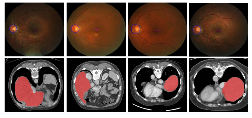
Figure 7: Examples of our semi-supervised (20%) segmentation results for the fundus image and liver CT scans. Blue color denotes the segmented boundary of optic disc and red color represents the segmented liver.

IV-E Experiments on LiTS dataset

For this dataset, we evaluate the performance of liver segmentation from CT volumes. Under our semi-supervised setting, we randomly separated the original 131 training data from the challenge into 121 training volumes and 10 testing volumes. For image preprocessing, we truncated the image intensity values of all scans to the range of [-200, 250] HU to remove the irrelevant details. We run experiments with 3D U-Net [41] to verify the effectiveness of our method. For the 3D U-Net, the input size is randomly cropped to $112\times 112\times 32$ to leverage the information from the third dimension.

According to the evaluation of the 2017 LiTS challenge, we employed Dice per case score to evaluate the liver segmentation result, which refers to an average Dice score per volume. We report the performance of our method and the other three semi-supervised methods under the settings of 10% labeled training images and 20% labeled training images, respectively, in Table VII. We can see that our approach achieves the highest performance improvement in both the 10% and 20% labeled training settings, with 5.33% and 5.72% improvements, respectively. In semi-supervised learning, it is obvious that our method gains higher performance consistently than other methods  [28, 18, 59, 52] in both 10% and 20% settings, respectively. We also visualize some liver segmentation results from CT scans in the second row of Figure 7.

V Discussion

Supervised deep learning has been proven extremely effective for many problems in the medical image community. However, promising performance heavily relies on the amount of annotations. Developing new methods with limited annotation will largely advance real-world clinical applications. In this work, we focus on developing semi-supervised learning methods for medical image segmentation, which have great potential to reduce the annotation effort by taking advantage of numerous unlabeled data. The key insight of our semi-supervised learning method is the transformation-consistent self-ensembling strategy. Extensive experiments on three representative and challenging datasets demonstrated the effectiveness of our method.

Medical image data has different formats, e.g., 2D in-plane scans (e.g., dermoscopy images and fundus images) and 3D volumetric data (e.g., MRI, CT). In this paper, we use both 2D and 3D networks for segmentation. Our method is flexible and can be easily applied to both 2D and 3D networks. It is worth noting that recent works [4, 30] are specifically designed for 3D volume data by considering three-view co-training, i.e., the coronal, sagittal and axial views of the volume data. However, we aim for a more general approach that is applicable to 2D and 3D medical images. For 3D semi-supervised learning, it could be a promising direction to design specific methods by considering the 3D natural property of the volumetric data.

Recent works on network equivariance [23, 31, 32] improve the generalization capacity of trained networks by exploring the equivariance property. E.g., Cohen and Welling [31] presented a group equivariant neural network. Our method also leverages the transformation consistency principle, but differently, we aim for semi-supervised segmentation. Moreover, if we trained these works, i.e., harmonic network [23], in a semi-supervised way to leverage unlabeled data, the transformation regularization will have no effect ideally, since the network outputs are the same when applying the transformation to the input images. Hence, the limited regularization would restrict the performance improvement from unlabeled data.

One limitation of our method is that we assume both labeled and unlabeled data come from the same distribution. However, in clinical applications, labeled and unlabeled data may have different distributions with a domain shift. Oliver et al. [65] demonstrated that the performance of semi-supervised learning methods can degrade substantially when the unlabeled dataset contains out-of-distribution samples. However, most of the current semi-supervised approaches for medical image segmentation do not consider this issue. Therefore, in the future, we would explore domain adaptation [10], and investigate how to adopt it with a self-ensembling strategy.

In our work, the selection of transformation is based on the property of neural networks. The convolution layer is not rotation equivariant. To tackle the segmentation task, we need to train the network to be rotation equivariant. Moreover, the neural network is not scale equivariant due to padding, upsampling, etc. The rotation and scaling transformations are the general transformations used in medical images. Thus, learning to minimize the output differences caused by these transformations will regularize the network to be transformation-consistent. Our method is flexible to extend to more general transformation cases, such as affine transformations. The transformation-consistent module consists of a transformation on the input image that will be fed to the teacher model, and the same transformation on the output space generated by the student model. It is flexible without additional training costs to be applied to the neural network. Moreover, recent automatic augmentation search works [66, 67, 68] explored the best transformations for a specific dataset. It is an interesting future work to explore more useful transformations for our semi-supervised segmentation framework through automatic data augmentation. Also, the experiments reported are the averaged result over three trials, which also indicates the robustness of our method.

VI Conclusion

This paper presents a novel and effective transformation-consistent self-ensembling semi-supervised method for medical image segmentation. The whole framework is trained with a teacher-student scheme and optimized by a weighted combination of supervised and unsupervised losses. To achieve this, we introduce a transformation-consistent self-ensembling model for the segmentation task, enhancing the regularization and can be easily applied on 2D and 3D networks. Comprehensive experimental analysis on three medical imaging datasets, i.e., skin lesion, retinal image, and liver CT datasets, demonstrated the effectiveness of our method. Our method is general and can be widely used in other semi-supervised medical imaging problems.

References

- Nie et al. [2018a] D. Nie, L. Wang, Y. Gao, J. Lian, and D. Shen, “Strainet: Spatially varying stochastic residual adversarial networks for mri pelvic organ segmentation,” IEEE transactions on neural networks and learning systems, vol. 30, no. 5, pp. 1552–1564, 2018.
- Mahmud et al. [2018] M. Mahmud, M. S. Kaiser, A. Hussain, and S. Vassanelli, “Applications of deep learning and reinforcement learning to biological data,” IEEE transactions on neural networks and learning systems, vol. 29, no. 6, pp. 2063–2079, 2018.
- Kohli et al. [2017] M. D. Kohli, R. M. Summers, and J. R. Geis, “Medical image data and datasets in the era of machine learning—whitepaper from the 2016 c-mimi meeting dataset session,” Journal of digital imaging, vol. 30, no. 4, pp. 392–399, 2017.
- Zhou et al. [2019] Y. Zhou, Y. Wang, P. Tang, S. Bai, W. Shen, E. Fishman, and A. Yuille, “Semi-supervised 3d abdominal multi-organ segmentation via deep multi-planar co-training,” in WACV. IEEE, 2019, pp. 121–140.
- Sedai et al. [2017] S. Sedai, D. Mahapatra, and S. e. a. Hewavitharanage, “Semi-supervised segmentation of optic cup in retinal fundus images using variational autoencoder,” in MICCAI. Springer, 2017, pp. 75–82.
- Cheplygina et al. [2019] V. Cheplygina, M. de Bruijne, and J. P. Pluim, “Not-so-supervised: a survey of semi-supervised, multi-instance, and transfer learning in medical image analysis,” Medical image analysis, vol. 54, pp. 280–296, 2019.
- Hu et al. [2018] Y. Hu, M. Modat, E. Gibson, W. Li, N. Ghavami, E. Bonmati et al., “Weakly-supervised convolutional neural networks for multimodal image registration,” Medical image analysis, vol. 49, pp. 1–13, 2018.
- Gondal et al. [2017] W. M. Gondal, J. M. Köhler, R. Grzeszick, G. A. Fink, and M. Hirsch, “Weakly-supervised localization of diabetic retinopathy lesions in retinal fundus images,” in 2017 IEEE International Conference on Image Processing (ICIP). IEEE, 2017, pp. 2069–2073.
- Feng et al. [2017] X. Feng, J. Yang, A. F. Laine, and E. D. Angelini, “Discriminative localization in cnns for weakly-supervised segmentation of pulmonary nodules,” in MICCAI. Springer, 2017, pp. 568–576.
- Kamnitsas et al. [2017] K. Kamnitsas, C. Baumgartner, C. Ledig, V. Newcombe, J. Simpson, A. Kane et al., “Unsupervised domain adaptation in brain lesion segmentation with adversarial networks,” in International conference on information processing in medical imaging. Springer, 2017, pp. 597–609.
- Dong et al. [2018] N. Dong, M. Kampffmeyer, X. Liang, Z. Wang, W. Dai, and E. Xing, “Unsupervised domain adaptation for automatic estimation of cardiothoracic ratio,” in MICCAI. Springer, 2018, pp. 544–552.
- Mahmood et al. [2018] F. Mahmood, R. Chen, and N. J. Durr, “Unsupervised reverse domain adaptation for synthetic medical images via adversarial training,” IEEE transactions on medical imaging, vol. 37, no. 12, pp. 2572–2581, 2018.
- You et al. [2011] X. You, Q. Peng, Y. Yuan, Y.-m. Cheung, and J. Lei, “Segmentation of retinal blood vessels using the radial projection and semi-supervised approach,” Pattern Recognition, vol. 44, no. 10-11, pp. 2314–2324, 2011.
- Portela et al. [2014] N. M. Portela, G. D. Cavalcanti, and T. I. Ren, “Semi-supervised clustering for mr brain image segmentation,” Expert Systems with Applications, vol. 41, no. 4, pp. 1492–1497, 2014.
- Masood et al. [2015] A. Masood, A. Al-Jumaily, and K. Anam, “Self-supervised learning model for skin cancer diagnosis,” in International IEEE EMBS Conference on Neural Engineering. IEEE, 2015, pp. 1012–1015.
- Gu et al. [2017] L. Gu, Y. Zheng, R. Bise, I. Sato, N. Imanishi, and S. Aiso, “Semi-supervised learning for biomedical image segmentation via forest oriented super pixels (voxels),” in MICCAI. Springer, 2017, pp. 702–710.
- Jaisakthi et al. [2017] S. Jaisakthi, A. Chandrabose, and P. Mirunalini, “Automatic skin lesion segmentation using semi-supervised learning technique,” arXiv preprint, 2017.
- Bai et al. [2017] W. Bai, O. Oktay, and M. e. a. Sinclair, “Semi-supervised learning for network-based cardiac mr image segmentation,” in MICCAI. Springer, 2017, pp. 253–260.
- Nie et al. [2018b] D. Nie, Y. Gao, L. Wang, and D. Shen, “Asdnet: Attention based semi-supervised deep networks for medical image segmentation,” in MICCAI. Springer, 2018, pp. 370–378.
- Perone and Cohen-Adad [2018] C. S. Perone and J. Cohen-Adad, “Deep semi-supervised segmentation with weight-averaged consistency targets,” in Deep Learning in Medical Image Analysis and Multimodal Learning for Clinical Decision Support. Springer, 2018, pp. 12–19.
- Ganaye et al. [2018] P.-A. Ganaye, M. Sdika, and H. Benoit-Cattin, “Semi-supervised learning for segmentation under semantic constraint,” in MICCAI. Springer, 2018, pp. 595–602.
- Laine and Aila [2017] S. Laine and T. Aila, “Temporal ensembling for semi-supervised learning,” in ICLR, 2017.
- Worrall et al. [2017] D. E. Worrall, S. J. Garbin, D. Turmukhambetov, and G. J. Brostow, “Harmonic networks: Deep translation and rotation equivariance,” in CVPR, vol. 2, 2017.
- Li et al. [2018a] X. Li, L. Yu, H. Chen, C.-W. Fu, and P.-A. Heng, “Semi-supervised skin lesion segmentation via transformation consistent self-ensembling model,” BMVC, 2018.
- He et al. [2016] K. He, X. Zhang, S. Ren, and J. Sun, “Deep residual learning for image recognition,” in CVPR, 2016, pp. 770–778.
- Jegou et al. [2010] H. Jegou, M. Douze, and C. Schmid, “Product quantization for nearest neighbor search,” IEEE transactions on pattern analysis and machine intelligence, vol. 33, no. 1, pp. 117–128, 2010.
- He et al. [2015] K. He, X. Zhang, S. Ren, and J. Sun, “Spatial pyramid pooling in deep convolutional networks for visual recognition,” IEEE transactions on pattern analysis and machine intelligence, vol. 37, no. 9, pp. 1904–1916, 2015.
- Zhang et al. [2017] Y. Zhang, L. Yang, J. Chen, M. Fredericksen, D. P. Hughes, and D. Z. Chen, “Deep adversarial networks for biomedical image segmentation utilizing unannotated images,” in MICCAI. Springer, 2017, pp. 408–416.
- Chartsias et al. [2018] A. Chartsias, T. Joyce, G. Papanastasiou, S. Semple, M. Williams, D. Newby, R. Dharmakumar, and S. A. Tsaftaris, “Factorised spatial representation learning: application in semi-supervised myocardial segmentation,” in MICCAI. Springer, 2018, pp. 490–498.
- Xia et al. [2018] Y. Xia, F. Liu, D. Yang, J. Cai, L. Yu, Z. Zhu et al., “3d semi-supervised learning with uncertainty-aware multi-view co-training,” arXiv preprint arXiv:1811.12506, 2018.
- Cohen and Welling [2016] T. Cohen and M. Welling, “Group equivariant convolutional networks,” in ICML, 2016, pp. 2990–2999.
- Dieleman et al. [2016] S. Dieleman, J. D. Fauw, and K. Kavukcuoglu, “Exploiting cyclic symmetry in convolutional neural networks,” in ICML, 2016, pp. 1889–1898.
- Li et al. [2018b] X. Li, L. Yu, C.-W. Fu, and P.-A. Heng, “Deeply supervised rotation equivariant network for lesion segmentation in dermoscopy images,” pp. 235–243, 2018.
- Emre Celebi et al. [2013] M. Emre Celebi, Q. Wen, S. Hwang, H. Iyatomi, and G. Schaefer, “Lesion border detection in dermoscopy images using ensembles of thresholding methods,” Skin Research and Technology, vol. 19, no. 1, 2013.
- Heimann and Meinzer [2009] T. Heimann and H.-P. Meinzer, “Statistical shape models for 3d medical image segmentation: a review,” Medical image analysis, vol. 13, no. 4, pp. 543–563, 2009.
- He and Xie [2012] Y. He and F. Xie, “Automatic skin lesion segmentation based on texture analysis and supervised learning,” in ACCV. Springer, 2012, pp. 330–341.
- Sadri et al. [2013] A. R. Sadri, M. Zekri, S. Sadri, N. Gheissari, M. Mokhtari, and F. Kolahdouzan, “Segmentation of dermoscopy images using wavelet networks,” IEEE transactions on biomedical engineering, vol. 60, no. 4, pp. 1134–1141, 2013.
- Cheng et al. [2013] J. Cheng, J. Liu, Y. Xu, F. Yin, D. W. K. Wong, N.-M. Tan, D. Tao, C.-Y. Cheng, T. Aung, and T. Y. Wong, “Superpixel classification based optic disc and optic cup segmentation for glaucoma screening,” IEEE transactions on medical imaging, vol. 32, no. 6, pp. 1019–1032, 2013.
- Abramoff et al. [2007] M. D. Abramoff, W. L. Alward, E. C. Greenlee, L. Shuba, C. Y. Kim, J. H. Fingert, and Y. H. Kwon, “Automated segmentation of the optic disc from stereo color photographs using physiologically plausible features,” Investigative Ophthalmology & Visual Science, vol. 48, no. 4, pp. 1665–1673, 2007.
- Chlebus et al. [2018] G. Chlebus, A. Schenk, J. H. Moltz, B. van Ginneken, H. K. Hahn, and H. Meine, “Automatic liver tumor segmentation in ct with fully convolutional neural networks and object-based postprocessing,” Scientific reports, vol. 8, no. 1, p. 15497, 2018.
- Çiçek et al. [2016] Ö. Çiçek, A. Abdulkadir, S. S. Lienkamp, T. Brox, and O. Ronneberger, “3d u-net: learning dense volumetric segmentation from sparse annotation,” in MICCAI. Springer, 2016, pp. 424–432.
- Ronneberger et al. [2015] O. Ronneberger, P. Fischer, and T. Brox, “U-net: Convolutional networks for biomedical image segmentation,” in MICCAI. Springer, 2015, pp. 234–241.
- Milletari et al. [2016] F. Milletari, N. Navab, and S.-A. Ahmadi, “V-net: Fully convolutional neural networks for volumetric medical image segmentation,” in International Conference on 3D Vision. IEEE, 2016, pp. 565–571.
- Yu et al. [2017] L. Yu, H. Chen, Q. Dou, J. Qin, and P.-A. Heng, “Automated melanoma recognition in dermoscopy images via very deep residual networks,” IEEE transactions on medical imaging, vol. 36, no. 4, pp. 994–1004, 2017.
- Fu et al. [2018] H. Fu, J. Cheng, Y. Xu, C. Zhang, D. W. K. Wong, J. Liu, and X. Cao, “Disc-aware ensemble network for glaucoma screening from fundus image,” IEEE transactions on medical imaging, vol. 37, no. 11, pp. 2493–2501, 2018.
- Tan et al. [2017] J. H. Tan, U. R. Acharya, S. V. Bhandary, K. C. Chua, and S. Sivaprasad, “Segmentation of optic disc, fovea and retinal vasculature using a single convolutional neural network,” Journal of Computational Science, vol. 20, pp. 70–79, 2017.
- Lu et al. [2017] F. Lu, F. Wu, P. Hu, Z. Peng, and D. Kong, “Automatic 3d liver location and segmentation via convolutional neural network and graph cut,” International Journal of Computer Assisted Radiology and Surgery, vol. 12, no. 2, pp. 171–182, 2017.
- Yang et al. [2017] D. Yang, D. Xu, S. K. Zhou, B. Georgescu, M. Chen, S. Grbic, D. Metaxas, and D. Comaniciu, “Automatic liver segmentation using an adversarial image-to-image network,” in MICCAI. Springer, 2017, pp. 507–515.
- Yuan et al. [2017] Y. Yuan, M. Chao, and Y.-C. Lo, “Automatic skin lesion segmentation using deep fully convolutional networks with jaccard distance,” IEEE transactions on medical imaging, vol. 36, no. 9, pp. 1876–1886, 2017.
- Li et al. [2018c] X. Li, H. Chen, X. Qi, Q. Dou, C.-W. Fu, and P.-A. Heng, “H-denseunet: hybrid densely connected unet for liver and tumor segmentation from ct volumes,” IEEE transactions on medical imaging, vol. 37, no. 12, pp. 2663–2674, 2018.
- Sajjadi et al. [2016] M. Sajjadi, M. Javanmardi, and T. Tasdizen, “Regularization with stochastic transformations and perturbations for deep semi-supervised learning,” in NIPS, 2016, pp. 1163–1171.
- Tarvainen and Valpola [2017] A. Tarvainen and H. Valpola, “Mean teachers are better role models: Weight-averaged consistency targets improve semi-supervised deep learning results,” in NIPS, 2017, pp. 1195–1204.
- Huang et al. [2017] G. Huang, Z. Liu, L. Van Der Maaten, and K. Q. Weinberger, “Densely connected convolutional networks.” in CVPR, vol. 1, no. 2, 2017, p. 3.
- Kingma and Ba [2014] D. P. Kingma and J. Ba, “Adam: A method for stochastic optimization,” arXiv preprint arXiv:1412.6980, 2014.
- Paszke et al. [2017] A. Paszke, S. Gross, S. Chintala, G. Chanan, E. Yang, Z. DeVito, Z. Lin, A. Desmaison, L. Antiga, and A. Lerer, “Automatic differentiation in PyTorch,” in NIPS Autodiff Workshop, 2017.
- Codella et al. [2018] N. C. Codella, D. Gutman, M. E. Celebi, B. Helba, M. A. Marchetti, S. W. Dusza et al., “Skin lesion analysis toward melanoma detection: A challenge at the 2017 international symposium on biomedical imaging (isbi),” in ISBI. IEEE, 2018, pp. 168–172.
- Bilic et al. [2019] P. Bilic, P. F. Christ, E. Vorontsov, G. Chlebus, H. Chen, Q. Dou, C.-W. Fu, X. Han, P.-A. Heng, J. Hesser et al., “The liver tumor segmentation benchmark (lits),” arXiv preprint arXiv:1901.04056, 2019.
- Seo et al. [2019] H. Seo, C. Huang, M. Bassenne, R. Xiao, and L. Xing, “Modified u-net (mu-net) with incorporation of object-dependent high level features for improved liver and liver-tumor segmentation in ct images,” IEEE transactions on medical imaging, 2019.
- Hung et al. [2018] W.-C. Hung, Y.-H. Tsai, Y.-T. Liou, Y.-Y. Lin, and M.-H. Yang, “Adversarial learning for semi-supervised semantic segmentation,” BMVC, 2018.
- Yuan and Lo [2017] Y. Yuan and Y.-C. Lo, “Improving dermoscopic image segmentation with enhanced convolutional-deconvolutional networks,” IEEE journal of biomedical and health informatics, vol. 23, no. 2, pp. 519–526, 2017.
- Venkatesh et al. [2018] G. Venkatesh, Y. Naresh, S. Little, and N. E. O’Connor, “A deep residual architecture for skin lesion segmentation,” in OR 2.0 Context-Aware Operating Theaters, Computer Assisted Robotic Endoscopy, Clinical Image-Based Procedures, and Skin Image Analysis. Springer, 2018, pp. 277–284.
- Berseth [2017] M. Berseth, “Isic 2017-skin lesion analysis towards melanoma detection,” arXiv preprint, 2017.
- Bi et al. [2017] L. Bi, J. Kim, E. Ahn, and D. Feng, “Automatic skin lesion analysis using large-scale dermoscopy images and deep residual networks,” arXiv preprint, 2017.
- Orlando et al. [2020] J. I. Orlando, H. Fu, J. B. Breda, K. van Keer, D. R. Bathula, A. Diaz-Pinto et al., “Refuge challenge: A unified framework for evaluating automated methods for glaucoma assessment from fundus photographs,” Medical image analysis, vol. 59, p. 101570, 2020.
- Oliver et al. [2018] A. Oliver, A. Odena, C. Raffel, E. D. Cubuk, and I. J. Goodfellow, “Realistic evaluation of deep semi-supervised learning algorithms,” NIPS, 2018.
- Cubuk et al. [2019] E. D. Cubuk, B. Zoph, D. Mane, V. Vasudevan, and Q. V. Le, “Autoaugment: Learning augmentation strategies from data,” in CVPR, 2019, pp. 113–123.
- Lim et al. [2019] S. Lim, I. Kim, T. Kim, C. Kim, and S. Kim, “Fast autoaugment,” in NIPS, 2019, pp. 6662–6672.
- Buslaev et al. [2020] A. Buslaev, V. I. Iglovikov, E. Khvedchenya, A. Parinov, M. Druzhinin, and A. A. Kalinin, “Albumentations: fast and flexible image augmentations,” Information, vol. 11, no. 2, p. 125, 2020.