Abstract

We investigate a distributed optimal control problem for a diffuse interface model for tumor growth. The model consists of a Cahn–Hilliard type equation for the phase field variable, a reaction diffusion equation for the nutrient concentration and a Brinkman type equation for the velocity field. These PDEs are endowed with homogeneous Neumann boundary conditions for the phase field variable, the chemical potential and the nutrient as well as a “no-friction” boundary condition for the velocity. The control represents a medication by cytotoxic drugs and enters the phase field equation. The aim is to minimize a cost functional of standard tracking type that is designed to track the phase field variable during the time evolution and at some fixed final time. We show that our model satisfies the basics for calculus of variations and we present first-order and second-order conditions for local optimality. Moreover, we present a globality condition for critical controls and we show that the optimal control is unique on small time intervals.

Keywords: Optimal control with PDEs, calculus of variations, tumor growth, Cahn–Hilliard equation, Brinkman equation, first-order necessary optimality conditions, second-order sufficient optimality conditions, uniqueness of globally optimal solutions.

MSC Classification: 35K61, 76D07, 49J20, 92C50.

1 Introduction

The evolution of cancer cells is influenced by a variety of biological mechanisms like, e.g., cell-cell adhesion or mechanical stresses, see [4]. Although cancer is one of the most common causes of death, the knowledge about underlying processes is still at an unsatisfying level. Due to the complexity of the evolution, experimental and medical research may not be sufficient to predict growth and to establish general treatment strategies. Thus, it is of high importance to develop biologically realistic and predictive mathematical models to identify the influence of different growth factors and mechanisms and to set up individual treatment.
In the recent past, diffuse interface models gained much interest (e.g., [23, 29, 33, 34]) and some of them seem to compare well with clinical data, see [1, 4, 21]. Typically, these models are derived from balance equations for mass and momentum and they incorporate exchange of mass and momentum between the phases. Mechanisms like chemotaxis, necrosis, angiogenesis and apoptosis can be included or effects due to viscoelasticity and stress, see e.g. [15, 28, 40].

In general, living biological tissues behave like viscoelastic fluids, see [11]. Since relaxation times of elastic materials are rather short (see [25]), it is reasonable to consider Stokes flow as an approximation of those tissues, see e.g., [19]. Indeed, many authors used Stokes flow to describe the tumor as a viscous fluid, see [20, 22]. In classical tumor growth models, velocities are modeled with the help of Darcy’s law. In these models the velocity is assumed to be proportional to the pressure gradient caused by the birth of new cells and by the deformation of the tissue, see [8, 32]. Brinkman’s law is an interpolation between the viscous fluid and the Darcy-type models, see e.g., [42, 53].

Introduction of the model.
In this paper, we consider the following model: Let $\Omega\subset\mathbb{R}^{d}$ with $d=2,3,$ be a bounded domain. For a fixed final time $T>0$, we write ${\Omega_{T}}:=\Omega\times(0,T)$. By $\mathbf{n}$ we denote the outer unit normal on $\partial\Omega$ and $\partial_{\mathbf{n}}g\coloneqq\nabla g\cdot\mathbf{n}$ denotes the outward normal derivative of the function $g$ on $\Gamma$. Our state system is given by

$$\textnormal{div}(\mathbf{v}) =(P\sigma-A)\mathds{h}(\varphi) \text{in}\;{\Omega_{T}},$$ (1a)

$$-\textnormal{div}(\mathbf{T}(\mathbf{v},p))+\nu\mathbf{v} =(\mu+\chi\sigma)\nabla\varphi \text{in}\;{\Omega_{T}},$$ (1b)

$$\partial_{t}\varphi+\textnormal{div}(\varphi\mathbf{v}) =m\Delta\mu+(P\sigma-A-u)\mathds{h}(\varphi) \text{in}\;{\Omega_{T}},$$ (1c)

$$\mu =-\epsilon\Delta\varphi+\epsilon^{-1}\psi^{\prime}(\varphi)-\chi\sigma \text{in}\;{\Omega_{T}},$$ (1d)

$$-\Delta\sigma+\mathds{h}(\varphi)\sigma =b(\sigma_{B}-\sigma) \text{in}\;{\Omega_{T}},$$ (1e)

$$\partial_{\mathbf{n}}\mu=\partial_{\mathbf{n}}\varphi=\partial_{\mathbf{n}}\sigma =0 \text{in}\;{\Gamma_{T}},$$ (1f)

$$\mathbf{T}(\mathbf{v},p)\mathbf{n} =0 \text{in}\;{\Gamma_{T}},$$ (1g)

$$\varphi(0) =\varphi_{0} \text{in}\;\Omega,$$ (1h)

where the viscous stress tensor is defined by

$$\mathbf{T}(\mathbf{v},p)\coloneqq 2\eta{\mathbf{D}}\mathbf{v}+\lambda\textnormal{div}(\mathbf{v})\mathbf{I}-p\mathbf{I},$$ (2)

and the symmetric velocity gradient is given by

$${\mathbf{D}}\mathbf{v}\coloneqq\tfrac{1}{2}(\nabla\mathbf{v}+\nabla\mathbf{v}^{T}).$$

In (1), we denote by $\varphi$ the difference of volume fractions of tumor tissue and healthy tissue where $\{x\in\Omega:\varphi(x)=1\}$ represents the region of unmixed tumor tissue, $\{x\in\Omega:\varphi(x)=-1\}$ stands for the surrounding healthy tissue. The volume-averaged velocity of the mixture and the pressure are denoted by $\mathbf{v}$ and $p$, respectively. The tumor consumes an unknown species $\sigma\in[0,1]$ acting as a nutrient like e.g. oxygen or glucose. Furthermore, $\mu$ denotes the chemical potential associated with $\varphi$. The mobility is represented by a positive constant $m$, the diffuse interface thickness is proportional to a small parameter $\epsilon>0$ and the constant $\nu>0$ is related to the fluid porosity. The shear and bulk viscosities are given by a positive constant $\eta$ and a non-negative constant $\lambda$, respectively. The non-negative constants $P$, $A$ and $\chi$ represent the proliferation rate, the apoptosis rate and the chemotaxis parameter, respectively. By $\sigma_{B}$, we denote the nutrient concentration in a preexisting vasculature and $b$ is a positive constant. Hence, the term $b(\sigma_{B}-\sigma)$ models the nutrient supply from the blood vessels if $\sigma_{B}>\sigma$ and the nutrient transport away from the domain for $\sigma_{B}<\sigma$. The term $-u\mathds{h}(\varphi)$ in (1c) models the elimination of tumor cells by cytotoxic drugs and the function $u$ will act as our control. Since it does not play any role in the analysis, we set $\epsilon=1$.
We investigate the following distributed optimal control problem:

$$\text{Minimize}\quad I(\varphi,\mu,\sigma,\mathbf{v},p,u) :=\frac{\upalpha_{0}}{2}\lVert\varphi(T)-\varphi_{f}\rVert_{L^{2}}^{2}+\frac{\upalpha_{1}}{2}\lVert\varphi-\varphi_{d}\rVert_{L^{2}(\Omega_{T})}^{2}+\frac{\kappa}{2}\lVert u\rVert_{L^{2}(\Omega_{T})}^{2}$$

subject to the control constraint

$$u\in\mathbb{U}:=\big{\{}u\in L^{2}(L^{2})\;\big{|}\;\bar{a}(x,t)\leq u(x,t)\leq\bar{b}(x,t)\;\;\text{for almost every}\;(x,t)\in{\Omega_{T}}\big{\}}$$ (3)

for box-restrictions $\bar{a},\bar{b}\in L^{2}(L^{2})$ and the state system (1). Here, $\upalpha_{0},\upalpha_{1}$ and $\kappa$ are nonnegative constants.
The optimal control problem can be interpreted as the search for a strategy how to supply a medication such that a desired evolution $\varphi_{d}$ and a therapeutic target $\varphi_{f}$ are achieved in the best possible way without causing harm to the patient (expressed by both the control constraint and the last term in the cost functional). The ratio between the parameters $\upalpha_{0}$, $\upalpha_{1}$ and $\kappa$ can be adjusted according to the importance of the individual therapeutic targets.
In the case when $\mathds{h}(-1)=0$, the term $-u\mathds{h}(\varphi)$ models the elimination of tumor cells by a supply of cytotoxic drugs represented by the control $u$. This specific control term has been investigated in [18] and also in [27] where a simpler model was studied in which the influence of the velocity $\mathbf{v}$ is neglected. However, in some situations it may be more reasonable to control, for instance, the evolution at the interface and one has to use a different form for $\mathds{h}(\cdot)$, see Remark 1 below. Therefore, we allow $\mathds{h}(\cdot)$ to be rather general.
Summary of our main results.
In Section 3, we prove the existence of a control-to-state operator that maps any admissible control $u\in\mathbb{U}$ onto a corresponding unique strong solution of the state equation (1). Furthermore, we show that this control-to-state operator is Lipschitz-continuous, Fréchet differentiable and satisfies a weak compactness property. In particular, we establish the fundamental requirements for calculus of variations.
In Section 4, we investigate the adjoint system. Its solution, that is called the adjoint state or the costate, is an important tool in optimal control theory as it provides a better description of optimality conditions. We prove the existence of a control-to-costate operator which maps any admissible control onto its corresponding adjoint state. Then, we show that this control-to-costate operator is Lipschitz continuous and Fréchet differentiable.
Eventually, in Section 5, we investigate the above optimal control problem. First, we show that there exists at least one globally optimal solution. After that, we establish first-order necessary conditions for local optimality. These conditions are of great importance for possible numerical implementations as they provide the foundation for many computational optimization methods. We also present a second-order sufficient condition for strict local optimality, a globality criterion for critical controls and a uniqueness result for the optimal control on small time intervals.
Comparison with the results established in [18].
We want to outline the main features and novelties of our work, especially compared to the results in [18]. The main difference lies in the equation for the nutrient concentration. In [18] the equation

$$-\Delta\sigma+\mathds{h}(\varphi)\sigma=0\quad\text{in }\Omega_{T},\qquad\partial_{\mathbf{n}}\sigma=K(1-\sigma)\quad\text{on }{\Gamma_{T}}$$ (4)

was used where $K$ denotes some positive boundary permeability constant. However, in this paper, we use equation (1e) endowed with a homogeneous Neumann boundary condition (as studied in [27]) to describe the nutrient distribution.
Apart from the fact that (1e) might be more reasonable in some situations from a modeling point of view, it provides some advantages with regard to analysis and optimal control theory. In particular, Lipschitz continuity and Fréchet differentiability of both the control-to-state operator and the control-to-costate operator can be established in much better function spaces. As a consequence, we can prove that the cost functional $J$ is twice continuously differentiable which was not possible in [18]. This enables us to establish second-order conditions for (strict) local optimality.
Finally, we want to comment on the fact that active transport is neglected in (4). In principle, it is possible to decouple the effects of chemotaxis and active transport, see, e.g., [29]. If the ratio between nutrient diffusion and active transport timescale is quite small, a non-dimensionalization argument together with the decoupling justifies the fact that active transport may be neglected, cf. [26].
Moreover, as mentioned above, we present a globality criterion for critical controls as well as a uniqueness result for the optimal control on small time intervals. These new conditions have neither been established in [18] nor for related models in the literature. However, we are convinced that analogous conditions could also be proved for the optimal control problem in [18].
Related results in the literature.
Finally, we want to mention further works where optimal control problems for tumor models are studied. Results on optimal control problems for tumor models based on ODEs are investigated in [39, 41, 43, 49]. In the context of PDE-based control problems we refer to [5] where a tumor growth model of advection-reaction-diffusion type is considered. There are various papers analyzing optimal control problems for Cahn–Hilliard equations (e.g., [12, 35, 44, 46, 45]). Furthermore, control problems for the convective Cahn–Hilliard equation where the control acts as a velocity were investigated in [14, 31, 51, 52] whereas in [6, 24] the control enters in the momentum equation of a Cahn–Hilliard–Navier–Stokes system. As far as control problems for Cahn–Hilliard-based models for tumor growth are considered, there are only a few contributions where an equation for the nutrient is included in the system. In [13], the authors investigated an optimal control problem consisting of a Cahn–Hilliard-type equation coupled to a time-dependent reaction-diffusion equation for the nutrient, where the control acts as a right-hand side in this nutrient equation. The model they considered was firstly proposed in [33] and later well-posedness and existence of strong solutions were established in [23]. However, effects due to velocity are not included in their model and mass conservation holds for the sum of tumor and nutrient concentrations. A similar model has been analyzed in [10] both from the viewpoint of optimal long-term and finite-time treatment of medication. Furthermore, we want to cite the paper [27] about an optimal control problem of treatment time where the control represents a medication of cytotoxic drugs and enters the phase field equation in the same way as ours. Although their nutrient equation is non-stationary, some of the major difficulties do not occur since the velocity is assumed to be negligible ($\mathbf{v}=\mathbf{0}$). Lastly, we want to mention the work [48], where the authors tackled an optimal control problem for a Cahn–Hilliard–Darcy model describing tumor growth in two space dimensions. However, this model neglects the influence of nutrients and poses a compatibility condition for the source term in the divergence equation resulting from a different boundary condition for the velocity. In particular, the source term does not depend on additional variables such as $\varphi$.

2 Preliminaries

At first, we want to fix some notation: For any (real) Banach space $X$, its corresponding norm is denoted by $\lVert\,\cdot\,\rVert_{X}$. We write $X^{\ast}$ to denote the dual space of $X$ and $\langle\cdot{,}\cdot\rangle_{X}$ to denote duality pairing between $X^{\ast}$ and $X$. If $X$ is endowed with an inner product, this product is denoted by $(\cdot{,}\cdot)_{X}$. The scalar product of two matrices is defined by

$$\mathbf{A}:\mathbf{B}\coloneqq\sum_{j,k=1}^{d}a_{jk}b_{jk}\quad\text{for }\mathbf{A}=(a_{ij})_{1\leq i,j\leq d},\;\mathbf{B}=(b_{ij})_{1\leq i,j\leq d}\in\mathbb{R}^{d\times d}.$$

For the standard Lebesgue and Sobolev spaces with $1\leq p\leq\infty$ and $k>0$, we use the notation $L^{p}\coloneqq L^{p}(\Omega)$ and $W^{k,p}\coloneqq W^{k,p}(\Omega)$. Their corresponding norms are denoted by $\lVert\,\cdot\,\rVert_{L^{p}}$ and $\lVert\,\cdot\,\rVert_{W^{k,p}}$. If $p=2$ we write $H^{k}\coloneqq W^{k,2}$ and $\lVert\,\cdot\,\rVert_{H^{k}}\coloneqq\lVert\,\cdot\,\rVert_{W^{k,2}}$. Sometimes, we will also write $\lVert\,\cdot\,\rVert_{p}$ instead of $\lVert\,\cdot\,\rVert_{L^{p}(L^{p})}$. Moreover, we write $\mathbf{L}^{p}$, $\mathbf{W}^{k,p}$ and $\mathbf{H}^{k}$ to denote the corresponding spaces of vector or matrix valued functions. For Bochner spaces, we use the notation $L^{p}(X)\coloneqq L^{p}(0,T;X)$ for any Banach space $X$ and $p\in[1,\infty]$. For the dual space $X^{\ast}$ of a Banach space $X$, we define the (generalized) mean value by

$$v_{\Omega}\coloneqq\frac{1}{|\Omega|}\int_{\Omega}v\;\mathrm{d}x\quad\text{for }v\in L^{1},\quad v_{\Omega}^{\ast}\coloneqq\frac{1}{|\Omega|}\langle v{,}1\rangle_{X}\quad\text{for }v\in X^{\ast}.$$

Furthermore, we define the following function spaces:

$$L_{0}^{2}\coloneqq\{w\in L^{2}\colon w_{\Omega}=0\},\quad(H^{1})_{0}^{\ast}\coloneqq\{f\in(H^{1})^{\ast}\colon f_{\Omega}^{\ast}=0\},\quad H_{\mathbf{n}}^{2}\coloneqq\{w\in H^{2}\colon\partial_{\mathbf{n}}w=0\text{ on }\partial\Omega\}.$$

We remark that the Neumann-Laplace operator $-\Delta_{N}\colon H^{1}\cap L_{0}^{2}\to(H^{1})_{0}^{\ast}$ is positive definite and self-adjoint. In particular, due to the Lax-Milgram theorem and the Poincaré inequality, its inverse operator $(-\Delta_{N})^{-1}\colon(H^{1})_{0}^{\ast}\to H^{1}\cap L_{0}^{2}$ is well-defined and we write $v\coloneqq(-\Delta_{N})^{-1}f$ for ${f\in(H^{1})_{0}^{\ast}}$ if $v_{\Omega}=0$ and

$$-\Delta v=f\text{ in }\Omega,\quad\partial_{\mathbf{n}}v=0\text{ on }\partial\Omega.$$

The embeddings $H_{\mathbf{n}}^{2}\hookrightarrow H^{1}\hookrightarrow L^{2}\simeq(L^{2})^{\ast}\hookrightarrow(H^{1})^{\ast}\hookrightarrow(H_{\mathbf{n}}^{2})^{\ast}$ are continuous. Therefore we can identify $\langle u{,}v\rangle_{H^{1}}=(u{,}v)_{L^{2}}$, $\langle u{,}w\rangle_{H^{2}}=(u{,}w)_{L^{2}}$ for all $u\in L^{2},\leavevmode\nobreak\ v\in H^{1}$ and $w\in H_{\mathbf{n}}^{2}$.
Eventually, we introduce the function spaces

$${\mathcal{V}}_{1} \coloneqq\big{(}H^{1}(L^{2})\cap L^{\infty}(H^{2})\cap L^{2}(H^{4})\big{)}\times\big{(}L^{\infty}(L^{2})\cap L^{2}(H^{2})\big{)}\times L^{\infty}(H^{2})\times L^{8}(\mathbf{H}^{2})\times L^{8}(H^{1}),$$

$${\mathcal{V}}_{2} \coloneqq L^{8}(\mathbf{L}^{2})\times L^{8}(H^{1})\times L^{2}(L^{2})\times\big{(}L^{\infty}(L^{2})\cap L^{2}(H^{2})\big{)}\times L^{\infty}(L^{2}),$$

$$V_{3} \coloneqq\big{(}H^{1}((H^{1})^{*})\cap L^{\infty}(H^{1})\cap L^{2}(H^{3})\big{)}\times L^{2}(H^{1})\times L^{2}(H^{2})\times L^{2}(\mathbf{H}^{2})\times L^{2}(H^{1}),$$

$${\mathcal{V}}_{4} \coloneqq H^{1}\times L^{2}(L^{6/5})\times L^{2}(H^{1})\times L^{2}(L^{2})\times L^{2}(\mathbf{H}^{1})\times L^{2}(\mathbf{L}^{2}),$$

endowed with their standard norms.

Moreover, we make the following assumptions which we will use in the rest of this paper:
Assumptions.

1. The domain $\Omega\subset\mathbb{R}^{d},\leavevmode\nobreak\ d=2,3,$ is bounded with $C^{4}-$boundary $\Gamma:=\partial\Omega$. Moreover the initial datum $\varphi_{0}\in H^{2}_{\mathbf{n}}$ and $\sigma_{B}\in C([0,T];L^{2})$ are given functions.

2. The constants $T$, $\eta$, $\nu$, $m$, $b$ are positive and the constants $P$, $A$, $\lambda$, $\chi$ are nonnegative.

3. The non-negative function $\mathds{h}$ belongs to $C^{3}_{b}(\mathbb{R})$, i.e., $\mathds{h}$ is bounded, three times continuously differentiable and its first, second and third-order derivatives are bounded. Without loss of generality, we assume that $|\mathds{h}|\leq 1$.

4. $\psi$ is the smooth double-well potential, i.e., $\psi(s):=\frac{1}{4}(s^{2}-1)^{2}$ for all $s\in\mathbb{R}$.

Remark 1.

 

1. In principal, it would be possible to consider more general potentials $\psi(\cdot)$. However, since the double-well potential is the classical choice for Cahn–Hilliard-type equations (apart from singular potentials like the logarithmic or double-obstacle potential) and to avoid being too technical, we focus on the above choice for $\psi$ in this work.

2. For the function $\mathds{h}(\cdot)$, there are two choices which are quite popular in the literature. In, e.g., [26, 29], the choice for $\mathds{h}$ is given by

   $$\mathds{h}(\varphi)=\max\Big{\{}0,\min\left\{1,\tfrac{1}{2}(1+\varphi)\right\}\Big{\}}\quad\forall\varphi\in\mathbb{R},$$

   satisfying $\mathds{h}(-1)=0$, $\mathds{h}(1)=1$. Other authors preferred to assume that $\mathds{h}$ is only active on the interface, i.e., for values of $\varphi$ between $-1$ and $1$, which motivates functions of the form

   $$\mathds{h}(\varphi)=\max\Big{\{}0,\tfrac{1}{2}(1-\varphi^{2})\Big{\}}\quad\text{or}\quad\mathds{h}(\varphi)=\tfrac{1}{2}\Big{(}\cos\big{(}\pi\min\big{\{}1,\max\{\varphi,-1\}\big{\}}\big{)}+1\Big{)},$$

   see, e.g., [34, 36]. Surely, we would have to use regularized versions of these choices to fulfill (A3).

3. We want to point out that the analysis for singular potentials is quite delicate, even for the uncontrolled version of (1), since source terms are present. In contrast to, for example, [46] where the estimates for $\mu$ are obtained from the energy due to an additional regularization term $\alpha\partial_{t}\mu$ (with $\alpha>0$) in (1c), our analysis is based on an estimate for the mean value of $\mu$. Clearly, if $\psi(\cdot)$ is singular, such an estimate is quite hard to obtain. Following the arguments, for instance, in [7], it is crucial to prove that $\frac{1}{|\Omega|}\int_{\Omega}\varphi(t)\;\mathrm{d}x\in(-1,1)$ for almost every $t\in(0,T)$.
   Since our model does not have the property of mass conservation for the phase field $\varphi$, we would require additional assumptions on the source terms and an argument such as used in [30]. However, this argument does not work when using source terms, for example, as in [34, 36] (see (b)) in combination with the double obstacle potential, which can be seen as follows: If there was a solution to (1) that fulfills $(\varphi(t_{*}))_{\Omega}=1$ for some $t_{*}\in(0,T)$, then $(\varphi(t))_{\Omega}=1$ for all $t\in[t_{*},T]$.

3 The control-to-state operator and its properties

We consider the system (1) as presented in the introduction. The first step is to define a set of controls that are admissible for our problem. Then we show that each of these admissible controls induces a unique strong solution (the so-called state) of the system (1). Thus, we can define a control-to-state-operator which maps any admissible control onto its corresponding state. We show that this operator has several important properties that are essential for calculus of variations: It is Lipschitz-continuous, Fréchet-differentiable and weakly compactness in some suitable sense.

3.1 The set of admissible controls

The set of admissible controls is defined as follows:

Definition 2.

Let $\bar{a},\bar{b}\in L^{2}(L^{2})$ be arbitrary fixed functions with $\bar{a}\leq\bar{b}$ almost everywhere in ${\Omega_{T}}$. Then the set

$$\mathbb{U}:=\big{\{}u\in L^{2}(L^{2})\;\big{|}\;\bar{a}(x,t)\leq u(x,t)\leq\bar{b}(x,t)\;\;\text{for almost every}\;(x,t)\in{\Omega_{T}}\big{\}}$$ (5)

is referred to as the set of admissible controls. Its elements are called admissible controls.

Note that this box-restricted set of admissible controls $\mathbb{U}$ is a non-empty, bounded subset of the Hilbert space $L^{2}(L^{2})$ since for all $u\in\mathbb{U}$,

$$\lVert u\rVert_{L^{2}(L^{2})}<\lVert\bar{a}\rVert_{L^{2}(L^{2})}+\lVert\bar{b}\rVert_{L^{2}(L^{2})}+1=:R.$$ (6)

This means that

$$\mathbb{U}\subsetneq\mathbb{U}_{R}\quad\text{with}\quad\mathbb{U}_{R}:=\big{\{}u\in L^{2}(L^{2})\;\big{|}\;\lVert u\rVert_{L^{2}(L^{2})}<R\big{\}}.$$ (7)

Obviously, the set $\mathbb{U}$ is also convex and closed in $L^{2}(L^{2})$. Therefore, it is weakly sequentially compact (see [50, Thm. 2.11]).

3.2 Strong solutions and uniform bounds

We can show that the system (1) has a unique strong solution for every control $u\in\mathbb{U}_{R}$:

Proposition 3.

Let $u\in\mathbb{U}_{R}$ be arbitrary. Then, there exists a strong solution quintuplet $(\varphi_{u},\mu_{u},\sigma_{u},\mathbf{v}_{u},p_{u})\in{\mathcal{V}}_{1}$ of (1). Moreover, every strong solution $(\varphi_{u},\mu_{u},\sigma_{u},\mathbf{v}_{u},p_{u})$ satisfies the following bounds that are uniform in $u$:

$$\lVert(\varphi_{u},\mu_{u},\sigma_{u},\mathbf{v}_{u},p_{u})\rVert_{{\mathcal{V}}_{1}}\leq C_{1},$$ (8)

where $C_{1}>0$ is a constant that depends only on on $R$, $\Omega$ and $T$ and the system parameters.

• The assertion follows with slight modifications in the proof of [18, Thm. 4]. We will sketch the main differences in the following:

Step 1:

Testing (1e) with $\sigma$, using (1f), the non-negativity of $\mathds{h}(\cdot)$ and Hölder’s and Young’s inequalities, we obtain

$$\int_{\Omega}|\nabla\sigma|^{2}\;\mathrm{d}x+b\int_{\Omega}|\sigma|^{2}{\mathrm{d}}x\leq\frac{b}{2}\int_{\Omega}|\sigma|^{2}+|\sigma_{B}|^{2}\;\mathrm{d}x,$$

meaning

$$\lVert\sigma\rVert_{H^{1}}\leq C\lVert\sigma_{B}\rVert_{L^{2}}.$$ (9)

Then, with exactly the same arguments as in [18, Proof of Thm. 4] it follows that

$$\lVert\varphi\rVert_{H^{1}((H^{1})^{*})\cap L^{\infty}(H^{1})\cap L^{4}(H^{2})\cap L^{2}(H^{3})}+\lVert\sigma\rVert_{L^{4}(H^{1})}+\lVert\mu\rVert_{L^{2}(H^{1})\cap L^{4}(L^{2})}$$

$$\quad+\lVert\textnormal{div}(\varphi\mathbf{v})\rVert_{L^{2}(L^{2})}+\lVert\mathbf{v}\rVert_{L^{\frac{8}{3}}(\mathbf{H}^{1})}+\lVert p\rVert_{L^{2}(L^{2})}\leq C,$$ (10)

with a constant $C$ depending only on the system parameters and on $\Omega$, $T$ and $R$.

Step 2:

Now, we want to establish higher order estimates. Using elliptic regularity theory, the assumptions on $\mathds{h}(\cdot)$ and $\sigma_{B}$, (1e)-(1g), (9) and (10), it is easy to check that

$$\lVert\sigma\rVert_{L^{\infty}(H^{2})}\leq C.$$ (11)

Together with the boundedness of $\mathds{h}(\cdot)$ and the Sobolev embedding $H^{2}\subset L^{\infty}$, this implies

$$\lVert\sigma\rVert_{L^{\infty}(L^{\infty})}+\lVert\textnormal{div}(\mathbf{v})\rVert_{L^{\infty}(L^{\infty})}+\lVert(P\sigma-A)\mathds{h}(\varphi)\rVert_{L^{\infty}(L^{\infty})}\leq C.$$ (12)

Testing (1c) with $\Delta^{2}\varphi$, (1c) with $m\Delta^{3}\varphi$, integrating by parts and summing the resulting identities, we obtain

$$\frac{{\mathrm{d}}}{{\mathrm{d}}t}\frac{1}{2}\int_{\Omega}|\Delta\varphi|^{2}\;\mathrm{d}x+m\int_{\Omega}|\Delta^{2}\varphi|^{2}\;\mathrm{d}x =\int_{\Omega}\big{(}(P\sigma-A-u)\mathds{h}(\varphi)-\textnormal{div}(\varphi\mathbf{v})\big{)}\Delta^{2}\varphi{\mathrm{d}}x$$

$$\quad+\int_{\Omega}m\Delta(\psi^{\prime}(\varphi)-\chi\sigma)\Delta^{2}\varphi\;\mathrm{d}x.$$ (13)

Due to Hölder’s and Young’s inequalities and (10)-(12), the Sobolev embedding $\mathbf{H}^{1}\subset\mathbf{L}^{6}$ and elliptic estimates, it follows that

$$\left|\int_{\Omega}\big{(}(P\sigma-A-u)\mathds{h}(\varphi)-\textnormal{div}(\varphi\mathbf{v})-m\chi\Delta\sigma\big{)}\Delta^{2}\varphi\;\mathrm{d}x\right| \leq C\lVert u\rVert_{L^{2}}^{2}+C\lVert v\rVert_{\mathbf{H}^{1}}^{2}\left(1+\lVert\Delta\varphi\rVert_{L^{2}}^{2}\right)+\frac{m}{4}\lVert\Delta^{2}\varphi\rVert_{L^{2}}^{2}.$$ (14)

Now, we observe that

$$\Delta(\psi^{\prime}(\varphi))=\psi^{\prime\prime\prime}(\varphi)|\nabla\varphi|^{2}+\psi^{\prime\prime}(\varphi)\Delta\varphi.$$

Using Hölder’s, Young’s and Gagliardo-Nirenberg’s inequalities, the assumptions on $\psi(\cdot)$, elliptic regularity theory and (10), this implies

$$\left|\int_{\Omega}m\Delta(\psi^{\prime}(\varphi))\Delta^{2}\varphi{\mathrm{d}}x\right| \leq C\left(1+\lVert\varphi\rVert_{L^{\infty}}^{4}+\lVert\varphi\rVert_{L^{\infty}}^{2}\lVert\nabla\varphi\rVert_{\mathbf{L}^{3}}^{2}\right)(1+\lVert\Delta\varphi\rVert_{L^{2}}^{2})+\frac{m}{2}\lVert\Delta^{2}\varphi\rVert_{L^{2}}^{2}$$

$$\leq C\left(1+\lVert\varphi\rVert_{H^{3}}^{2}\right)\left(1+\lVert\Delta\varphi\rVert_{L^{2}}^{2}\right)+\frac{m}{2}\lVert\Delta^{2}\varphi\rVert_{L^{2}}^{2}.$$ (15)

Using (14)-(15) in (13), recalling (10) and using elliptic regularity theory, a Gronwall argument yields

$$\lVert\varphi\rVert_{L^{\infty}(H^{2})}+\lVert\varphi\rVert_{L^{2}(H^{4})}\leq C.$$ (16)

Then, a comparison argument in (1d) yields

$$\lVert\mu\rVert_{L^{\infty}(L^{2})\cap L^{2}(H^{2})}\leq C.$$ (17)

A further comparison argument in (1c) yields

$$\lVert\partial_{t}\varphi\rVert_{L^{2}(L^{2})}\leq C.$$ (18)

Using (10)-(12), (16)-(17), the assumptions on $\mathds{h}(\cdot)$ and Gagliardo-Nirenberg’s inequality, it is easy to check that

$$\lVert(P\sigma-A)\mathds{h}(\varphi)\rVert_{L^{8}(H^{1})}\leq C,\qquad\lVert(\mu+\chi\sigma)\nabla\varphi\rVert_{L^{8}(\mathbf{L}^{2})}\leq C.$$

Due to [16, Lemma 1.5], this implies

$$\lVert\mathbf{v}\rVert_{L^{8}(\mathbf{H}^{2})}+\lVert p\rVert_{L^{8}(H^{1})}\leq C,$$ (19)

which completes the proof. ∎

By means of interpolation theory, we can conclude that the $\varphi$-component of a strong solution quintuplet has a representative that is continuous on ${\Omega_{T}}$.

Corollary 4.

Let $u\in\mathbb{U}_{R}$ and $\varphi_{0}\in H^{2}_{\mathbf{n}}(\Omega)$ be arbitrary and let $(\varphi_{u},\mu_{u},\sigma_{u},\mathbf{v}_{u},p_{u})$ denote the strong solution of the system (1). Then, $\varphi_{u}$ has the following additional properties:

$$\varphi_{u}\in C([0,T];H^{2}),\quad\varphi_{u}\in C(\overline{{\Omega_{T}}})\quad\text{with}\quad\lVert\varphi_{u}\rVert_{C([0,T];H^{2})\cap C(\overline{{\Omega_{T}}})}\leq C_{2}$$

for some constant $C_{2}>0$ that depends only on the system parameters and on $R$, $\Omega$, $\Gamma$ and $T$.

• The assertion can be established by an interpolation argument. The proof proceeds completely analogously to the proof of [18, Cor. 5]. ∎

Furthermore, we can show that any control $u\in\mathbb{U}_{R}$ induces a unique strong solution of the system (1):

Theorem 5.

Let $u\in\mathbb{U}_{R}$ and $\varphi_{0}\in H^{2}_{\mathbf{n}}(\Omega)$ be arbitrary and let $(\varphi_{u},\mu_{u},\mathbf{v}_{u},\sigma_{u},p_{u})$ denote the corresponding strong solution as given by Proposition 3. Then, this strong solution is unique.

• Let $u,{\tilde{u}}\in\mathbb{U}_{R}$ be arbitrary and let $C$ denote a generic nonnegative constant that depends only on $R$, $\Omega$, $\Gamma$ and $T$ and may change its value from line to line. For brevity, we set

  $$(\varphi,\mu,\mathbf{v},\sigma,p):=(\varphi_{u},\mu_{u},\mathbf{v}_{u},\sigma_{u},p_{u})-(\varphi_{\tilde{u}},\mu_{\tilde{u}},\mathbf{v}_{\tilde{u}},\sigma_{\tilde{u}},p_{\tilde{u}}).$$

  where $(\varphi_{u},\mu_{u},\mathbf{v}_{u},\sigma_{u},p_{u})$ and $(\varphi_{\tilde{u}},\mu_{\tilde{u}},\mathbf{v}_{\tilde{u}},\sigma_{\tilde{u}},p_{\tilde{u}})$ are strong solutions of (1) to the controls $u$ and ${\tilde{u}}$. In particular, this means that both strong solutions satisfy the initial condition (1h), i.e., $\varphi_{u}(\cdot,0)=\varphi_{\tilde{u}}(\cdot,0)=\varphi_{0}$ holds almost everywhere in $\Omega$.
  

  Then, the following equations are satisfied:

  $$\textnormal{div}(\mathbf{v}) =P\sigma\mathds{h}(\varphi_{u})+(P\sigma_{\tilde{u}}-A)(\mathds{h}(\varphi_{u})-\mathds{h}(\varphi_{\tilde{u}})) \text{in}\;{\Omega_{T}},$$ (20a)

  $$-\textnormal{div}(\mathbf{T}(\mathbf{v},p))+\nu\mathbf{v} =(\mu+\chi\sigma)\nabla\varphi_{u}+(\mu_{\tilde{u}}+\chi\sigma_{\tilde{u}})\nabla\varphi \text{in}\;{\Omega_{T}},$$ (20b)

  $$\partial_{t}\varphi+\textnormal{div}(\varphi_{u}\mathbf{v})+\textnormal{div}(\varphi\mathbf{v}_{\tilde{u}}) =m\Delta\mu+P\sigma\mathds{h}(\varphi_{u})+(P\sigma_{\tilde{u}}-A)(\mathds{h}(\varphi_{u})-\mathds{h}(\varphi_{\tilde{u}}))$$

  $$\quad-(u\mathds{h}(\varphi_{u})-{\tilde{u}}\mathds{h}(\varphi_{\tilde{u}})) \text{in}\;{\Omega_{T}},$$ (20c)

  $$\mu =-\Delta\varphi+(\psi^{\prime}(\varphi_{u})-\psi^{\prime}(\varphi_{\tilde{u}}))-\chi\sigma \text{in}\;{\Omega_{T}},$$ (20d)

  $$-\Delta\sigma+b\sigma+\mathds{h}(\varphi_{u})\sigma =-\sigma_{\tilde{u}}(\mathds{h}(\varphi_{u})-\mathds{h}(\varphi_{\tilde{u}})) \text{in}\;{\Omega_{T}},$$ (20e)

  $$\partial_{\mathbf{n}}\mu=\partial_{\mathbf{n}}\varphi=\partial_{\mathbf{n}}\sigma =0 \text{in}\;{\Gamma_{T}},$$ (20f)

  $$\mathbf{T}(\mathbf{v},p)\mathbf{n} =0 \text{in}\;{\Gamma_{T}},$$ (20g)

  $$\varphi(0) =0 \text{in}\;\Omega.$$ (20h)

  Now, we will show that $\lVert(\varphi,\mu,\mathbf{v},\sigma,p)\rVert_{{\mathcal{V}}_{1}}=0$ if $u={\tilde{u}}$. The argumentation is split into two steps:

Step 1:

In [18], it has been shown that the following inequalities hold: For any $\delta>0$ and all $u,{\tilde{u}}\in\mathbb{U}$,

$$\big{|}\big{(}u\mathds{h}(\varphi_{u})-{\tilde{u}}\mathds{h}(\varphi_{\tilde{u}}){,}\varphi\big{)}_{L^{2}}\big{|} \leq C\,\lVert u-{\tilde{u}}\rVert_{L^{2}}^{2}+C\,\lVert\varphi\rVert_{L^{2}}^{2}+C\,\lVert{\tilde{u}}\rVert_{L^{2}}\lVert\varphi\rVert_{H^{1}}^{2},$$ (21)

$$\big{|}\big{(}u\mathds{h}(\varphi_{u})-{\tilde{u}}\mathds{h}(\varphi_{\tilde{u}}){,}\Delta\varphi\big{)}_{L^{2}}\big{|} \leq C\delta^{-1}\,\lVert u-{\tilde{u}}\rVert_{L^{2}}^{2}+C\delta^{-1}\,\lVert{\tilde{u}}\rVert_{L^{2}}^{2}\lVert\varphi\rVert_{H^{1}}^{2}+2\delta\lVert\Delta\varphi\rVert_{L^{2}}^{2}+\delta\lVert\nabla\Delta\varphi\rVert_{\mathbf{L}^{2}}^{2}.$$ (22)

Now, multiplying (20e) with $\sigma$, integrating by parts and using (20f), it follows that

$$\int_{\Omega}|\nabla\sigma|^{2}+b|\sigma|^{2}+\mathds{h}(\varphi_{u})|\sigma|^{2}\;\mathrm{d}x=-\int_{\Omega}\sigma_{\tilde{u}}(h(\varphi_{u})-\mathds{h}(\varphi_{\tilde{u}}))\sigma\;\mathrm{d}x.$$

Using the assumptions on $\mathds{h}(\cdot)$, Proposition 3 and Hölder’s and Young’s inequalities, it is therefore easy to check that

$$\lVert\sigma\rVert_{H^{1}}\leq C\lVert\varphi\rVert_{L^{2}}.$$ (23)

Then, we can follow the arguments in [17, Sec. 5] to deduce that

$$\lVert\varphi\rVert_{H^{1}((H^{1})^{*})\cap L^{\infty}(H^{1})\cap L^{2}(H^{3})}+\lVert\mu\rVert_{L^{2}(H^{1})}+\lVert\sigma\rVert_{L^{2}(H^{1})}+\lVert\mathbf{v}\rVert_{L^{2}(\mathbf{H}^{1})}+\lVert p\rVert_{L^{2}(L^{2})}\leq C\lVert u-{\tilde{u}}\rVert_{L^{2}(L^{2})}.$$ (24)

Step 2:

We now prove higher order estimates. Using elliptic regularity theory, Proposition 3, (23)-(24) and the assumptions on $\mathds{h}(\cdot)$, it is easy to check that

$$\lVert\sigma\rVert_{L^{\infty}(H^{2})}\leq C\lVert u-{\tilde{u}}\rVert_{L^{2}(L^{2})}.$$ (25)

Multiplying (20c) with $\Delta^{2}\varphi$ and inserting the expression for $\mu$ given by (20d), we obtain

$$\frac{{\mathrm{d}}}{\;\mathrm{d}t}\frac{1}{2}\int_{\Omega}|\Delta\varphi|^{2}\;\mathrm{d}x+m\int_{\Omega}|\Delta^{2}\varphi|^{2}\;\mathrm{d}x =\int_{\Omega}\big{(}P\sigma\mathds{h}(\varphi_{u})+(P\sigma_{\tilde{u}}-A)(\mathds{h}(\varphi_{u})-\mathds{h}(\varphi_{\tilde{u}}))\big{)}\Delta^{2}\varphi\;\mathrm{d}x$$

$$\quad-\int_{\Omega}\big{(}\textnormal{div}(\varphi_{u}\mathbf{v})+\textnormal{div}(\varphi\mathbf{v}_{\tilde{u}})\big{)}\Delta^{2}\varphi\;\mathrm{d}x$$

$$\quad+m\int_{\Omega}\Delta\big{(}(\psi^{\prime}(\varphi_{u})-\psi^{\prime}(\varphi_{\tilde{u}}))-\chi\sigma\big{)}\Delta^{2}\varphi\;\mathrm{d}x$$

$$\quad-\int_{\Omega}(u\mathds{h}(\varphi_{u})-{\tilde{u}}\mathds{h}(\varphi_{\tilde{u}}))\Delta^{2}\varphi\;\mathrm{d}x,$$ (26)

where we used that

$$\int_{\Omega}\partial_{t}\varphi\,\Delta^{2}\varphi\;\mathrm{d}x=\frac{{\mathrm{d}}}{\;\mathrm{d}t}\frac{1}{2}\int_{\Omega}|\Delta\varphi|^{2}\;\mathrm{d}x\quad\forall\varphi\in H^{2}(L^{2})\cap L^{2}(H^{4}),\quad\partial_{\mathbf{n}}\varphi=\partial_{\mathbf{n}}\Delta\varphi=0.$$

Using Proposition 3, (24)-(25) together with Hölder’s and Young’s inequalities, it follows that

$$\left|\int_{\Omega}\big{(}P\sigma\mathds{h}(\varphi_{u})+(P\sigma_{\tilde{u}}-A)(\mathds{h}(\varphi_{u})-\mathds{h}(\varphi_{\tilde{u}}))-\textnormal{div}(\varphi_{u}\mathbf{v})-\textnormal{div}(\varphi\mathbf{v}_{\tilde{u}})-m\chi\Delta\sigma\big{)}\Delta^{2}\varphi\;\mathrm{d}x\right|$$

$$\quad\leq C\left(\lVert\mathbf{v}\rVert_{\mathbf{H}^{1}}^{2}+\lVert\varphi\rVert_{H^{1}}^{2}\lVert\mathbf{v}_{\tilde{u}}\rVert_{\mathbf{H}^{2}}^{2}+\lVert\sigma\rVert_{H^{2}}^{2}+\lVert\varphi\rVert_{L^{2}}^{2}\right)+\frac{m}{8}\lVert\Delta^{2}\varphi\rVert_{L^{2}}^{2}.$$ (27)

Using the continuous embedding $H^{2}\subset L^{\infty}$, Proposition 3, (24), the assumptions on $\mathds{h}(\cdot)$ and the elliptic estimate

$$\lVert\varphi\rVert_{H^{2}}\leq C\left(\lVert\varphi\rVert_{L^{2}}+\lVert\Delta\varphi\rVert_{L^{2}}\right)\quad\forall\varphi\in H_{\mathbf{n}}^{2},$$

we obtain

$$\left|\int_{\Omega}(u\mathds{h}(\varphi_{u})-{\tilde{u}}\mathds{h}(\varphi_{\tilde{u}}))\Delta^{2}\varphi\;\mathrm{d}x\right| =\left|\int_{\Omega}\big{(}(u-{\tilde{u}})\mathds{h}(\varphi_{u})+{\tilde{u}}(\mathds{h}(\varphi_{u})-h(\varphi_{\tilde{u}}))\big{)}\Delta^{2}\varphi\;\mathrm{d}x\right|$$

$$\leq C\left(\lVert u-{\tilde{u}}\rVert_{L^{2}}+\lVert{\tilde{u}}\rVert_{L^{2}}(\lVert\varphi\rVert_{L^{2}}+\lVert\Delta\varphi\rVert_{L^{2}})\right)\lVert\Delta^{2}\varphi\rVert_{L^{2}}$$

$$\leq C\left(\lVert u-{\tilde{u}}\rVert_{L^{2}}^{2}+\lVert{\tilde{u}}\rVert_{L^{2}}^{2}(\lVert\varphi\rVert_{L^{2}}^{2}+\lVert\Delta\varphi\rVert_{L^{2}}^{2})\right)+\frac{m}{8}\lVert\Delta^{2}\varphi\rVert_{L^{2}}^{2}.$$ (28)

Now, we observe that

$$\Delta(\psi^{\prime}(\varphi_{u})-\psi^{\prime}(\varphi_{\tilde{u}})) =\psi^{\prime\prime}(\varphi_{u})\Delta\varphi+\Delta\varphi_{\tilde{u}}(\psi^{\prime\prime}(\varphi_{u})-\psi^{\prime\prime}(\varphi_{\tilde{u}}))$$

$$\quad+\psi^{\prime\prime\prime}(\varphi_{u})\left(\nabla\varphi_{u}+\nabla\varphi_{\tilde{u}}\right)\left(\nabla\varphi_{u}-\nabla\varphi_{\tilde{u}}\right)+\left(\psi^{\prime\prime\prime}(\varphi_{u})-\psi^{\prime\prime\prime}(\varphi_{\tilde{u}})\right)|\nabla\varphi_{\tilde{u}}|^{2}.$$

Due to the assumptions on $\psi(\cdot)$ and because of Proposition 3, it is straightforward to check that

$$\int_{\Omega}|\psi^{\prime\prime}(\varphi_{u})\Delta\varphi|^{2}+|\Delta\varphi_{\tilde{u}}(\psi^{\prime\prime}(\varphi_{u})-\psi^{\prime\prime}(\varphi_{\tilde{u}}))|^{2}\;\mathrm{d}x\leq C\left(\lVert\varphi\rVert_{L^{2}}^{2}+\lVert\Delta\varphi\rVert_{L^{2}}^{2}\right),$$

where we used the continuous embedding $H^{2}\subset L^{\infty}$ and elliptic regularity theory. With similar argument, using the Sobolev embedding $\mathbf{H}^{1}\subset\mathbf{L}^{6}$ and the assumptions on $\psi(\cdot)$, we obtain

$$\int_{\Omega}|\psi^{\prime\prime\prime}(\varphi_{u})\left(\nabla\varphi_{u}+\nabla\varphi_{\tilde{u}}\right)\left(\nabla\varphi_{u}-\nabla\varphi_{\tilde{u}}\right)|^{2}+|\left(\psi^{\prime\prime\prime}(\varphi_{u})-\psi^{\prime\prime\prime}(\varphi_{\tilde{u}})\right)|^{2}|\nabla\varphi_{\tilde{u}}|^{4}\;\mathrm{d}x\leq C\left(\lVert\varphi\rVert_{L^{2}}^{2}+\lVert\Delta\varphi\rVert_{L^{2}}^{2}\right).$$

From the last two inequalities, we obtain

$$\lVert\Delta(\psi^{\prime}(\varphi_{u})-\psi^{\prime}(\varphi_{\tilde{u}}))\rVert_{L^{2}}^{2}\leq C\left(\lVert\varphi\rVert_{L^{2}}^{2}+\lVert\Delta\varphi\rVert_{L^{2}}^{2}\right).$$ (29)

Therefore, we have

$$\left|m\int_{\Omega}\Delta\big{(}(\psi^{\prime}(\varphi_{u})-\psi^{\prime}(\varphi_{\tilde{u}}))\big{)}\Delta^{2}\varphi\;\mathrm{d}x\right|\leq C\left(\lVert\varphi\rVert_{L^{2}}^{2}+\lVert\Delta\varphi\rVert_{L^{2}}^{2}\right)+\frac{m}{8}\lVert\Delta^{2}\varphi\rVert_{L^{2}}^{2}.$$ (30)

Plugging in (27)-(30) into (26), we obtain

$$\frac{{\mathrm{d}}}{\;\mathrm{d}t}\int_{\Omega}|\Delta\varphi|^{2}\;\mathrm{d}x+m\int_{\Omega}|\Delta^{2}\varphi|^{2}\;\mathrm{d}x \leq\left(\lVert\varphi\rVert_{L^{2}}^{2}+\lVert{\tilde{u}}\rVert_{L^{2}}^{2}\lVert\varphi\rVert_{L^{2}}^{2}+\lVert\mathbf{v}_{\tilde{u}}\rVert_{\mathbf{H}^{2}}^{2}\lVert\varphi\rVert_{H^{1}}^{2}+\lVert\sigma\rVert_{H^{2}}^{2}+\lVert\mathbf{v}\rVert_{\mathbf{H}^{1}}^{2}+\lVert u-{\tilde{u}}\rVert_{L^{2}}^{2}\right)$$

$$\qquad+C\left(1+\lVert{\tilde{u}}\rVert_{L^{2}}^{2}\right)\lVert\Delta\varphi\rVert_{L^{2}}^{2}.$$ (31)

Invoking Proposition 3 and (24) and using elliptic regularity theory, a Gronwall argument yields

$$\lVert\varphi\rVert_{H^{1}((H^{1})^{*})\cap L^{\infty}(H^{2})\cap L^{2}(H^{3})}+\lVert\Delta\varphi\rVert_{L^{2}(H^{2})}+\lVert\mu\rVert_{L^{2}(H^{1})}+\lVert\sigma\rVert_{L^{\infty}(H^{2})}+\lVert\mathbf{v}\rVert_{L^{2}(\mathbf{H}^{1})}+\lVert p\rVert_{L^{2}(L^{2})}$$

$$\quad\leq C\lVert u-{\tilde{u}}\rVert_{L^{2}(L^{2})}.$$ (32)

Using (29) and (3.2), a comparison argument in (20d) implies

$$\lVert\mu\rVert_{L^{\infty}(L^{2})\cap L^{2}(H^{2})}\leq C\lVert u-{\tilde{u}}\rVert_{L^{2}(L^{2})}.$$ (33)

Again using elliptic theory, from (20d), (20f) and (33) we obtain

$$\lVert\varphi\rVert_{L^{2}(H^{4})}\leq C\lVert u-{\tilde{u}}\rVert_{L^{2}(L^{2})}.$$ (34)

A further comparison argument in (20c) together with (33) yields

$$\lVert\partial_{t}\varphi\rVert_{L^{2}(L^{2})}\leq C\lVert u-{\tilde{u}}\rVert_{L^{2}(L^{2})}.$$ (35)

Summarising (3.2)-(35), we obtain

$$\lVert\varphi\rVert_{H^{1}(L^{2})\cap L^{\infty}(H^{2})\cap L^{2}(H^{4})}+\lVert\mu\rVert_{L^{\infty}(L^{2})\cap L^{2}(H^{2})}+\lVert\sigma\rVert_{L^{\infty}(H^{2})}+\lVert\mathbf{v}\rVert_{L^{2}(\mathbf{H}^{1})}+\lVert p\rVert_{L^{2}(L^{2})}\leq C\lVert u-{\tilde{u}}\rVert_{L^{2}(L^{2})}.$$ (36)

Together with the assumptions on $\mathds{h}(\cdot)$ and Gagliardo-Nirenberg’s inequality, it follows that

$$\lVert\textnormal{div}(\mathbf{v})\rVert_{L^{8}(H^{1})} \leq C\lVert u-{\tilde{u}}\rVert_{L^{2}(L^{2})},$$ (37)

$$\lVert(\mu+\chi\sigma)\nabla\varphi_{u}+(\mu_{\tilde{u}}+\chi\sigma_{\tilde{u}})\nabla\varphi\rVert_{L^{8}(\mathbf{L}^{2})} \leq C\lVert u-{\tilde{u}}\rVert_{L^{2}(L^{2})}.$$ (38)

Then, an application of [16, Lemma 1.5] yields

$$\lVert\mathbf{v}\rVert_{L^{8}(\mathbf{H}^{2})}+\lVert p\rVert_{L^{8}(H^{1})}\leq C\lVert u-{\tilde{u}}\rVert_{L^{2}(L^{2})}.$$ (39)

Together with (36), this implies that

$$\lVert(\varphi,\mu,\sigma,\mathbf{v},p)\rVert_{{\mathcal{V}}_{1}}\leq C\lVert u-{\tilde{u}}\rVert_{L^{2}(L^{2})}.$$ (40)

Hence, setting $u={\tilde{u}}$ completes the proof. ∎

Due to Proposition 3 and Theorem 5, we can define an operator that maps any control $u\in\mathbb{U}_{R}$ onto its corresponding state:

Definition 6.

For any $u\in\mathbb{U}_{R}$ we write $(\varphi_{u},\mu_{u},\sigma_{u},\mathbf{v}_{u},p_{u})$ to denote the corresponding unique strong solution of (1) given by Proposition 3. Then the operator

$$\mathcal{S}:\;\mathbb{U}_{R}\to{\mathcal{V}}_{1},\quad u\mapsto\mathcal{S}(u):=(\varphi_{u},\mu_{u},\sigma_{u},\mathbf{v}_{u},p_{u})$$

is called the control-to-state operator.

Remark 7.

The control-to-state operator is defined not only for admissible controls but for all controls in $\mathbb{U}_{R}$. This will be especially important in subsection 3.4 because Fréchet differentiability is merely defined for open subsets of $L^{2}(L^{2})$. Unlike the open ball $\mathbb{U}_{R}$, the set $\mathbb{U}$ is closed and its interior is empty. Therefore it makes sense to investigate the control-to-state operator on the open superset $\mathbb{U}_{R}$ instead.

In the following subsections, some properties of the control-to-state operator will be established that are essential for the treatment of optimal control problems.

3.3 Lipschitz continuity

The proof of Theorem 5 does actually provide more than uniqueness of strong solutions of (1). In fact, we have showed that the strong solution depends Lipschitz-continuously on the control.

Corollary 8.

The control-to-state operator $S\colon\mathbb{U}_{R}\to{\mathcal{V}}_{1}$ is Lipschitz continuous, i.e., there exists a constant $L_{1}>0$ depending only on the system parameters and on $R$, $\Omega$, $\Gamma$ and $T$ such that for all $u,{\tilde{u}}\in\mathbb{U}_{R}$:

$$\lVert\mathcal{S}(u)-\mathcal{S}({\tilde{u}})\rVert_{{\mathcal{V}}_{1}}\leq L_{1}\lVert u-{\tilde{u}}\rVert_{L^{2}(L^{2})}.$$ (41)

• The assertion follows directly from (40). ∎

3.4 A weak compactness property

As the control-to-state operator is nonlinear, the following result will be essential to prove existence of an optimal control (see Section 5.1):

Lemma 9.

Suppose that $(u_{k})_{k\in\mathbb{N}}\subset\mathbb{U}$ is converging weakly in $L^{2}(L^{2})$ to some limit ${\bar{u}}\in\mathbb{U}$. Then

$$\varphi_{u_{k}} \rightharpoonup\varphi_{\bar{u}}\quad \text{in}\;H^{1}(L^{2})\cap L^{2}(H^{4}),\quad \varphi_{u_{k}} \to\varphi_{\bar{u}} \text{in}\;C\big{(}[0,T];W^{1,r}\big{)}\cap C\big{(}\overline{{\Omega_{T}}}\big{)},\leavevmode\nobreak\ r\in[1,6),$$

$$\mu_{u_{k}} \rightharpoonup\mu_{\bar{u}}\quad \text{in}\;L^{2}(H^{2}), \mathbf{v}_{u_{k}} \rightharpoonup\mathbf{v}_{\bar{u}}\quad \text{in}\;L^{2}(\mathbf{H}^{2}),$$

$$\sigma_{u_{k}} \rightharpoonup\sigma_{\bar{u}}\quad \text{in}\;L^{2}(H^{2}),\quad p_{u_{k}} \rightharpoonup p_{\bar{u}}\quad \text{in}\;L^{2}(H^{1}),$$

after extraction of a subsequence, where the limit $(\varphi_{\bar{u}},\mu_{\bar{u}},\sigma_{\bar{u}},\mathbf{v}_{\bar{u}},p_{\bar{u}})$ is the strong solution of (1) to the control ${\bar{u}}\in\mathbb{U}$.

• The assertion follows with exactly the same arguments as the proof of [18, Lem. 8]. ∎

Remark 10.

This result actually means weak compactness of the control-to-state operator restricted to $\mathbb{U}$ since any bounded sequence in $\mathbb{U}$ has a weakly convergent subsequence according to the Banach-Alaoglu theorem. However, this property can not be considered as weak continuity as the extraction of a subsequence is necessary.

3.5 The linearized system

We want to show that the control-to-state operator is also Fréchet differentiable on the open ball $\mathbb{U}_{R}$ (and therefore especially on its strict subset $\mathbb{U}$). Since the Fréchet derivative is a linear approximation of the control-to-state operator at some certain point $u\in\mathbb{U}_{R}$, it will be given by a linearized version of (1):

$$\textnormal{div}(\mathbf{v}) =P\sigma\mathds{h}(\varphi_{u})+(P\sigma_{u}-A)\mathds{h}^{\prime}(\varphi_{u})\varphi+F_{1} \text{in}\;{\Omega_{T}},$$ (42a)

$$-\textnormal{div}(\mathbf{T}(\mathbf{v},p))+\nu\mathbf{v} =(\mu_{u}+\chi\sigma_{u})\nabla\varphi+(\mu+\chi\sigma)\nabla\varphi_{u}+{\mathbf{F}} \text{in}\;{\Omega_{T}},$$ (42b)

$$\partial_{t}\varphi+\textnormal{div}(\varphi_{u}\mathbf{v})+\textnormal{div}(\varphi\mathbf{v}_{u}) =m\Delta\mu+(P\sigma_{u}-A-u)\mathds{h}^{\prime}(\varphi_{u})\varphi$$

$$\qquad+P\sigma\mathds{h}(\varphi_{u})+F_{2} \text{in}\;{\Omega_{T}},$$ (42c)

$$\mu =-\Delta\varphi+\psi^{\prime\prime}(\varphi_{u})\varphi-\chi\sigma+F_{3} \text{in}\;{\Omega_{T}},$$ (42d)

$$-\Delta\sigma-b\sigma+\mathds{h}^{\prime}(\varphi_{u})\varphi\sigma_{u}+\mathds{h}(\varphi_{u})\sigma =F_{4} \text{in}\;{\Omega_{T}},$$ (42e)

$$\partial_{\mathbf{n}}\mu=\partial_{\mathbf{n}}\varphi=\partial_{\mathbf{n}}\sigma =0 \text{in}\;{\Gamma_{T}},$$ (42f)

$$\mathbf{T}(\mathbf{v},p)\mathbf{n} =0 \text{in}\;{\Gamma_{T}},$$ (42g)

$$\varphi(0) =0 \text{in}\;\Omega,$$ (42h)

where $F_{i}:{\Omega_{T}}\to\mathbb{R},\,1\leq i\leq 4$ and ${\mathbf{F}}:{\Omega_{T}}\to\mathbb{R}^{3}$ are given functions that will be specified later on. A strong solution of this linearized system is defined as follows:

Definition 11.

Let $u\in\mathbb{U}_{R}$ be arbitrary. Then a quintuplet $(\varphi,\mu,\sigma,\mathbf{v},p)$ is called a strong solution of (42) if it lies in ${\mathcal{V}}_{1}$ and satisfies (42) almost everywhere in the respective sets.

Existence and uniqueness of strong solutions to this linearized system is established by the following lemma:

Proposition 12.

Let $u\in\mathbb{U}_{R}$ be any control and let $(\varphi,\mu,\sigma,\mathbf{v},p)$ denote its corresponding state. Moreover, let $({\mathbf{F}},F_{1},F_{2},F_{3},F_{4})\in{\mathcal{V}}_{2}$ be arbitrary. Then the system (42) has a unique strong solution $(\varphi,\mu,\sigma,\mathbf{v},p)\in{\mathcal{V}}_{1}$. Moreover, there exists some constant $C>0$ depending only on the system parameters and on $R$, $\Omega$, $\Gamma$ and $T$ such that:

$$\lVert(\varphi,\mu,\sigma,\mathbf{v},p)\rVert_{{\mathcal{V}}_{1}}\leq C\lVert({\mathbf{F}},F_{1},F_{2},F_{3},F_{4})\rVert_{{\mathcal{V}}_{2}}.$$ (43)

• The proof can be carried out using a Galerkin scheme by constructing approximate solutions with respect to $\varphi$ and $\mu$ and at the same time solve for $\sigma,\,\mathbf{v}$ and $p$ in the corresponding whole function spaces. For the details, we refer to [18, Sec. 3.5] In the following steps, we will show a-priori-estimates for the solutions. All the estimates can be carried out rigorously within the Galerkin scheme. In the following approach, Hölder’s and Young’s inequalities will be used frequently.

Step 1:

Multiplying (42e) with $\sigma$, integrating by parts and using (42f), the boundedness of $\mathds{h}^{\prime}(\varphi_{u})\in L^{\infty}({\Omega_{T}}),\,\sigma_{u}\in L^{\infty}(L^{\infty})$ and the non-negativity of $\mathds{h}(\cdot)$ yields

$$\lVert\nabla\sigma\rVert_{\mathbf{L}^{2}}^{2}+b\lVert\sigma\rVert_{L^{2}}^{2}=\left|\int_{\Omega}\big{(}F_{4}-\mathds{h}^{\prime}(\varphi_{u})\varphi\sigma_{u}\big{)}\sigma\;\mathrm{d}x\right|\leq\delta_{1}\lVert\sigma\rVert_{H^{1}}^{2}+C_{\delta_{1}}\left(\lVert\varphi\rVert_{L^{2}}^{2}+\lVert F_{4}\rVert_{L^{2}}^{2}\right)$$

for $\delta_{1}>0$ arbitrary. Choosing $\delta_{8}=\frac{1}{2}\min\{1,b\}$, this implies that

$$\lVert\sigma\rVert_{H^{1}}\leq C\left(\lVert\varphi\rVert_{L^{2}}+\lVert F_{4}\rVert_{L^{2}}\right).$$ (44)

Then, using exactly the same arguments as in [18], it can be shown that

$$\lVert\varphi\rVert_{L^{\infty}(H^{1})\cap L^{2}(H^{3})}+\lVert\mu\rVert_{L^{2}(H^{1})}+\lVert\sigma\rVert_{L^{2}(H^{1})}+\lVert\mathbf{v}\rVert_{L^{2}(\mathbf{H}^{1})}+\lVert p\rVert_{L^{2}(L^{2})}$$

$$\quad\leq C\left(\lVert\nabla F_{3}\rVert_{L^{2}(\mathbf{L}^{2})}+\lVert{\mathbf{F}}\rVert_{L^{2}(\mathbf{L}^{2})}+\sum_{i=1}^{4}\lVert F_{i}\rVert_{L^{2}({\Omega_{T}})}\right).$$ (45)

Step 2:

We want to establish higher order estimates for $\varphi$, $\mu$ and $\sigma$. With (42e)-(42f) and elliptic regularity theory, it follows that

$$\lVert\sigma\rVert_{H^{2}}\leq C\left(\lVert\mathds{h}^{\prime}(\varphi_{u})\varphi\sigma_{u}\rVert_{L^{2}}+\lVert F_{4}\rVert_{L^{2}}\right).$$

Due to the assumptions on $\mathds{h}(\cdot)$, using Proposition 3 and (45) implies

$$\lVert\sigma\rVert_{L^{\infty}(H^{2})}\leq C\left(\lVert\nabla F_{3}\rVert_{L^{2}(\mathbf{L}^{2})}+\lVert{\mathbf{F}}\rVert_{L^{2}(\mathbf{L}^{2})}+\sum_{i=1}^{3}\lVert F_{i}\rVert_{L^{2}({\Omega_{T}})}+\lVert F_{4}\rVert_{L^{\infty}(L^{2})}\right).$$ (46)

We now multiply (42) with $\Delta^{2}\varphi$, integrate by parts and insert the expression for $\mu$ given by (42d) to obtain

$$\frac{{\mathrm{d}}}{\;\mathrm{d}t}\frac{1}{2}\int_{\Omega}|\Delta\varphi|^{2}\;\mathrm{d}x+m\int_{\Omega}|\Delta^{2}\varphi|^{2}\;\mathrm{d}x =\int_{\Omega}\big{(}(P\sigma_{u}-A-u)\mathds{h}^{\prime}(\varphi_{u})\varphi+P\sigma\mathds{h}(\varphi_{u})+F_{2}\big{)}\Delta^{2}\varphi\;\mathrm{d}x$$

$$\quad-\int_{\Omega}\big{(}\textnormal{div}(\varphi_{u}\mathbf{v})+\textnormal{div}(\varphi\mathbf{v}_{u})\big{)}\Delta^{2}\varphi\;\mathrm{d}x$$

$$\quad+m\int_{\Omega}\Delta\big{(}\psi^{\prime\prime}(\varphi_{u})\varphi-\chi\sigma+F_{3}\big{)}\Delta^{2}\varphi\;\mathrm{d}x.$$ (47)

Using Proposition 3, the assumptions on $\mathds{h}(\cdot)$, (46)-(47) and the continuous embeddings $H^{1}\subset L^{6},\,\mathbf{H}^{1}\subset\mathbf{L}^{6},\,\mathbf{H}^{2}\subset\mathbf{L}^{\infty}$, we have

$$\left|\int_{\Omega}\big{(}(P\sigma_{u}-A)\mathds{h}^{\prime}(\varphi_{u})\varphi+P\sigma\mathds{h}(\varphi_{u})+F_{2}-\textnormal{div}(\varphi_{u}\mathbf{v})+\textnormal{div}(\varphi\mathbf{v}_{u})\big{)}\Delta^{2}\varphi\;\mathrm{d}x\right|$$

$$\quad\leq C\left(1+\lVert\mathbf{v}_{u}\rVert_{\mathbf{H}^{2}}^{2}\right)\lVert\varphi\rVert_{H^{1}}^{2}+C\left(\lVert\sigma\rVert_{L^{2}}^{2}+\lVert\mathbf{v}\rVert_{\mathbf{H}^{1}}^{2}+\lVert F_{2}\rVert_{L^{2}}^{2}\right)+\frac{m}{8}\lVert\Delta^{2}\varphi\rVert_{L^{2}}^{2}.$$ (48)

Furthermore, it is straightforward to check that

$$\left|m\int_{\Omega}\Delta\big{(}-\chi\sigma+F_{3}\big{)}\Delta^{2}\varphi\;\mathrm{d}x\right|\leq C\left(\lVert\sigma\rVert_{H^{2}}^{2}+\lVert F_{3}\rVert_{H^{2}}^{2}\right)+\frac{m}{8}\lVert\Delta^{2}\varphi\rVert_{L^{2}}^{2}.$$ (49)

Now, using elliptic regularity theory, the Sobolev embedding $H^{2}\subset L^{\infty}$, the assumptions on $\mathds{h}(\cdot)$ and Proposition 3, we calculate

$$\left|\int_{\Omega}u\mathds{h}^{\prime}(\varphi_{u})\varphi\Delta^{2}\varphi\;\mathrm{d}x\right|\leq C\lVert u\rVert_{L^{2}}\lVert\varphi\rVert_{H^{2}}\lVert\Delta^{2}\varphi\rVert_{L^{2}}\leq C\lVert u\rVert_{L^{2}}^{2}\left(\lVert\varphi\rVert_{L^{2}}^{2}+\lVert\Delta\varphi\rVert_{L^{2}}^{2}\right)+\frac{m}{8}\lVert\Delta^{2}\varphi\rVert_{L^{2}}^{2}.$$ (50)

Next, we observe that

$$\Delta(\psi^{\prime\prime}(\varphi_{u})\varphi)=\psi^{(4)}(\varphi_{u})|\nabla\varphi_{u}|^{2}\varphi+\psi^{\prime\prime\prime}(\varphi_{u})\Delta\varphi_{u}\varphi+2\psi^{\prime\prime\prime}(\varphi_{u})\nabla\varphi_{u}\cdot\nabla\varphi+\psi^{\prime\prime}(\varphi_{u})\Delta\varphi.$$

Using the Sobolev embeddings $H^{1}\subset L^{6},\,H^{2}\subset L^{\infty},\,\mathbf{H}^{1}\subset\mathbf{L}^{6}$, the assumptions on $\psi(\cdot)$, Proposition 3 and elliptic regularity theory again, we obtain

$$\lVert\Delta(\psi^{\prime\prime}(\varphi_{u})\varphi)\rVert_{L^{2}}^{2}\leq C\left(\lVert\varphi\rVert_{L^{2}}^{2}+\lVert\Delta\varphi\rVert_{L^{2}}^{2}\right).$$ (51)

Consequently,

$$\left|m\int_{\Omega}\Delta(\psi^{\prime\prime}(\varphi_{u})\varphi)\Delta^{2}\varphi\;\mathrm{d}x\right|\leq C\lVert\Delta(\psi^{\prime\prime}(\varphi_{u})\varphi)\rVert_{L^{2}}^{2}+\frac{m}{8}\lVert\Delta^{2}\varphi\rVert_{L^{2}}^{2}\leq C\left(\lVert\varphi\rVert_{L^{2}}^{2}+\lVert\Delta\varphi\rVert_{L^{2}}^{2}\right)+\frac{m}{8}\lVert\Delta^{2}\varphi\rVert_{L^{2}}^{2}.$$ (52)

Plugging in (48)-(52) into (47), we obtain

$$\frac{{\mathrm{d}}}{\;\mathrm{d}t}\frac{1}{2}\int_{\Omega}|\Delta\varphi|^{2}\;\mathrm{d}x+\frac{m}{2}\int_{\Omega}|\Delta^{2}\varphi|^{2}\;\mathrm{d}x \leq C\left(1+\lVert\mathbf{v}_{u}\rVert_{\mathbf{H}^{2}}^{2}\right)\lVert\varphi\rVert_{H^{1}}^{2}+C\left(\lVert\sigma\rVert_{H^{2}}^{2}+\lVert\mathbf{v}\rVert_{\mathbf{H}^{1}}^{2}+\lVert F_{2}\rVert_{L^{2}}^{2}+\lVert F_{3}\rVert_{H^{2}}^{2}\right)$$

$$\quad+C\left(1+\lVert u\rVert_{L^{2}}^{2}\right)\left(\lVert\varphi\rVert_{L^{2}}^{2}+\lVert\Delta\varphi\rVert_{L^{2}}^{2}\right).$$

Integrating this inequality in time from $0$ to $T$, using (45)-(46), Proposition 3 and elliptic regularity theory, we end up with

$$\lVert\varphi\rVert_{L^{\infty}(H^{2})\cap L^{2}(H^{3})}+\lVert\Delta^{2}\varphi\rVert_{L^{2}(L^{2})}+\lVert\mu\rVert_{L^{2}(H^{1})}+\lVert\sigma\rVert_{L^{\infty}(H^{2})}+\lVert\mathbf{v}\rVert_{L^{2}(\mathbf{H}^{1})}+\lVert p\rVert_{L^{2}(L^{2})}$$

$$\quad\leq C\left(\lVert{\mathbf{F}}\rVert_{L^{2}(\mathbf{L}^{2})}+\sum_{i=1}^{2}\lVert F_{i}\rVert_{L^{2}({\Omega_{T}})}+\lVert F_{3}\rVert_{L^{2}(H^{2})}+\lVert F_{4}\rVert_{L^{\infty}(L^{2})}\right).$$ (53)

Now, using elliptic regularity theory and (42d), (42f), (51) and (53), we deduce that

$$\lVert\mu\rVert_{L^{2}(H^{2})}\leq C\left(\lVert{\mathbf{F}}\rVert_{L^{2}(\mathbf{L}^{2})}+\sum_{i=1}^{2}\lVert F_{i}\rVert_{L^{2}({\Omega_{T}})}+\lVert F_{3}\rVert_{L^{2}(H^{2})}+\lVert F_{4}\rVert_{L^{\infty}(L^{2})}\right).$$ (54)

Furthermore, using Proposition 3, the assumptions on $\psi(\cdot)$ and (53), a comparison argument in (42d) yields

$$\lVert\mu\rVert_{L^{\infty}(L^{2})}\leq C\,C_{F}$$ (55)

where

$$C_{F}\coloneqq\left(\lVert{\mathbf{F}}\rVert_{L^{2}(\mathbf{L}^{2})}+\sum_{i=1}^{2}\lVert F_{i}\rVert_{L^{2}({\Omega_{T}})}+\lVert F_{3}\rVert_{L^{\infty}(L^{2})\cap L^{2}(H^{2})}+\lVert F_{4}\rVert_{L^{\infty}(L^{2})}\right).$$ (56)

Now, using elliptic regularity, Proposition 3, the assumptions on $\psi(\cdot)$ and (51), (53), one can check that

$$\lVert\psi^{\prime\prime}(\varphi_{u})\varphi\rVert_{L^{2}(H^{2})}\leq C\,C_{F}.$$

Hence, using elliptic regularity theory again and recalling (53)-(54), from (42d) we deduce

$$\lVert\varphi\rVert_{L^{2}(H^{4})}\leq C\,C_{F}.$$ (57)

A further comparison in (42) together with (53)-(57) yields

$$\lVert\partial_{t}\varphi\rVert_{L^{2}(L^{2})}\leq C\,C_{F}.$$ (58)

Summarising (53)-(57), we showed that

$$\lVert\varphi\rVert_{H^{1}(L^{2})\cap L^{\infty}(H^{2})\cap L^{2}(H^{4})}+\lVert\mu\rVert_{L^{\infty}(L^{2})\cap L^{2}(H^{2})}+\lVert\sigma\rVert_{L^{\infty}(H^{2})}+\lVert\mathbf{v}\rVert_{L^{2}(\mathbf{H}^{1})}+\lVert p\rVert_{L^{2}(L^{2})}\leq C\,C_{F}.$$ (59)

Step 3:

Now, we also want to prove higher order estimates for $\mathbf{v}$ and $p$. Using Proposition 3, the assumptions on $\mathds{h}(\cdot)$ and (59), a straightforward calculation shows that

$$\lVert P\sigma\mathds{h}(\varphi_{u})+(P\sigma_{u}-A)\mathds{h}^{\prime}(\varphi_{u})\varphi\rVert_{L^{8}(H^{1})}\leq C\,C_{F}.$$ (60)

Using Gagliardo-Nirenberg’s inequality, we have the continuous embedding

$$L^{\infty}(\mathbf{H}^{1})\cap L^{2}(\mathbf{H}^{3})\hookrightarrow L^{8}(\mathbf{L}^{\infty}).$$

Together with Proposition 3 and (59), this implies that

$$\lVert(\mu_{u}+\chi\sigma_{u})\nabla\varphi+(\mu+\chi\sigma)\nabla\varphi_{u}\rVert_{L^{8}(\mathbf{L}^{2})}\leq C\,C_{F}.$$ (61)

Using (60)-(61) and recalling (59), an application of [16, Lemma 1.5] to (42a)-(42b), (42g) yields

$$\lVert(\varphi,\mu,\sigma,\mathbf{v},p)\rVert_{{\mathcal{V}}_{1}}\leq C\lVert({\mathbf{F}},F_{1},F_{2},F_{3},F_{4})\rVert_{{\mathcal{V}}_{2}},$$ (62)

hence we showed (43).

Step 4:

Due to (62), we can pass to the limit in the Galerkin scheme to deduce that (42) holds. The initial condition is attained due to the compact embedding $H^{1}((H^{1})^{*})\cap L^{\infty}(H^{1})\hookrightarrow C([0,T];L^{2})$ (see [47, sect. 8, Cor. 4]). Moreover, the estimate (43) results from the weak-star lower semicontinuity of the ${\mathcal{V}}_{1}$-norm. Finally, uniqueness follows from linearity of the system together with (43). ∎

3.6 Fréchet differentiability

Now, this result can be used to prove Fréchet differentiability of the control-to-state operator:

Proposition 13.

The following statements hold:

1. The control-to-state operator $S$ is Fréchet differentiable on $\mathbb{U}_{R}$, i.e., for any $u\in\mathbb{U}_{R}$ there exists a unique bounded linear operator

   $$\mathcal{S}^{\prime}(u):L^{2}(L^{2})\to{\mathcal{V}}_{1},\quad h\mapsto\mathcal{S}^{\prime}(u)[h]=\big{(}\varphi^{\prime}_{u},\mu^{\prime}_{u},\mathbf{v}^{\prime}_{u},\sigma^{\prime}_{u},p^{\prime}_{u}\big{)}[h],$$

   such that

   $$\frac{\lVert\mathcal{S}(u+h)-\mathcal{S}(u)-\mathcal{S}^{\prime}(u)[h]\rVert_{{\mathcal{V}}_{1}}}{\lVert h\rVert_{L^{2}(L^{2})}}\to 0\qquad\text{as}\;\lVert h\rVert_{L^{2}(L^{2})}\to 0.$$

   For any $u\in\mathbb{U}$ and $h\in L^{2}(L^{2})$, the Fréchet derivative $\big{(}\varphi^{\prime}_{u},\mu^{\prime}_{u},\mathbf{v}^{\prime}_{u},\sigma^{\prime}_{u},p^{\prime}_{u}\big{)}[h]$ is the unique strong solution of the system (42) with

   $$F_{1},F_{3},F_{4}=0,\quad{\mathbf{F}}=\mathbf{0}\quad\text{and}\quad F_{2}=-h\,\mathds{h}(\varphi_{u}).$$

2. The Frechet-derivative is Lipschitz continuous, i.e., for any $u,{\tilde{u}}\in\mathbb{U}_{R}$ and $h\in L^{2}(L^{2})$, it holds that

   $$\lVert\mathcal{S}^{\prime}(u)[\cdot]-\mathcal{S}^{\prime}({\tilde{u}})[\cdot]\rVert_{\mathcal{L}(L^{2}(L^{2});{\mathcal{V}}_{1})}\leq L_{2}\lVert u-{\tilde{u}}\rVert_{L^{2}(L^{2})},$$ (63)

   with a constant $L_{2}>0$ depending only on the system parameters and on $\Omega$, $T$, $R$.

• Let $C$ denote a generic nonnegative constant that depends only on $R$, $\Omega$ and $T$ and may change its value from line to line.

Proof of (i):

To prove Fréchet differentiability we must consider the difference

$$(\varphi,\mu,\sigma,\mathbf{v},p):=(\varphi_{u+h},\mu_{u+h},\mathbf{v}_{u+h},\sigma_{u+h},p_{u+h})-(\varphi_{u},\mu_{u},\sigma_{u},\mathbf{v}_{u},p_{u})$$

for some arbitrary $u\in\mathbb{U}_{R}$ and $h\in L^{2}(L^{2})$ with $u+h\in\mathbb{U}_{R}$. Therefore, we assume that $\lVert h\rVert_{L^{2}(L^{2})}<\delta$ for some sufficiently small $\delta>0$. Now, we Taylor expand the nonlinear terms in (1) to pick out the linear contributions. We obtain that

$$\mathds{h}(\varphi_{u+h})-\mathds{h}(\varphi_{u}) =\mathds{h}^{\prime}(\varphi_{u})\varphi+\mathcal{R}_{1},$$

$$\sigma_{u+h}\mathds{h}(\varphi_{u+h})-\sigma_{u}\mathds{h}(\varphi_{u}) =\sigma\mathds{h}(\varphi_{u})+\sigma_{u}\mathds{h}^{\prime}(\varphi_{u})\varphi+\mathcal{R}_{2},$$

$$(u+h)\mathds{h}(\varphi_{u+h})-u\mathds{h}(\varphi_{u}) =u\mathds{h}^{\prime}(\varphi_{u})\varphi+h\mathds{h}(\varphi_{u})+\mathcal{R}_{3},$$

$$(\mu_{u+h}+\chi\sigma_{u+h})\nabla\varphi_{u+h}-(\mu_{u}+\chi\sigma_{u})\nabla\varphi_{u} =(\mu_{u}+\chi\sigma_{u})\nabla\varphi+(\mu+\chi\sigma)\nabla\varphi_{u}+\mathcal{R}_{4},$$

$$\textnormal{div}(\varphi_{u+h}\mathbf{v}_{u+h})-\textnormal{div}(\varphi_{u}\mathbf{v}_{u}) =\textnormal{div}(\varphi\mathbf{v}_{u})+\textnormal{div}(\varphi_{u}\mathbf{v})+\mathcal{R}_{5},$$

$$\psi^{\prime}(\varphi_{u+h})-\psi^{\prime}(\varphi_{u}) =\psi^{\prime\prime}(\varphi_{u})\varphi+\mathcal{R}_{6},$$

where the nonlinear remainders are given by

$$\mathcal{R}_{1} :=\tfrac{1}{2}\mathds{h}^{\prime\prime}(\zeta)(\varphi_{u+h}-\varphi_{u})^{2},$$

$$\mathcal{R}_{2} :=(\sigma_{u+h}-\sigma_{u})(\mathds{h}(\varphi_{u+h})-\mathds{h}(\varphi_{u}))+\tfrac{1}{2}\sigma_{u}\mathds{h}^{\prime\prime}(\zeta)(\varphi_{u+h}-\varphi_{u})^{2},$$

$$\mathcal{R}_{3} :=\tfrac{1}{2}u\,\mathds{h}^{\prime\prime}(\zeta)(\varphi_{u+h}-\varphi_{u})^{2}+h\big{(}\mathds{h}(\varphi_{u+h})-\mathds{h}(\varphi_{u})\big{)},$$

$$\mathcal{R}_{4} :=\big{[}(\mu_{u+h}-\mu_{u})+\chi(\sigma_{u+h}-\sigma_{u})\big{]}(\nabla\varphi_{u+h}-\nabla\varphi_{u}),$$

$$\mathcal{R}_{5} :=\textnormal{div}\big{[}(\varphi_{u+h}-\varphi_{u})(\mathbf{v}_{u+h}-\mathbf{v}_{u})\big{]},$$

$$\mathcal{R}_{6} :=\tfrac{1}{2}\psi^{\prime\prime\prime}(\xi)(\varphi_{u+h}-\varphi_{u})^{2}$$

with $\zeta=\vartheta\varphi_{u+h}+(1-\vartheta)\varphi_{u}$ and $\xi=\theta\varphi_{u+h}+(1-\theta)\varphi_{u}$ for some $\vartheta,\theta\in[0,1]$. This means that the difference $(\varphi,\mu,\sigma,\mathbf{v},p)$ is the strong solution of (42) with

$$F_{1}=P\mathcal{R}_{2}-A\mathcal{R}_{1},\quad{\mathbf{F}}=\mathcal{R}_{4},\quad F_{2}=P\mathcal{R}_{2}-A\mathcal{R}_{1}-\mathcal{R}_{3}-\mathcal{R}_{5}-h\,\mathds{h}(\varphi_{u}),\quad F_{3}=\mathcal{R}_{6},\quad F_{4}=-\mathcal{R}_{2}.$$

By a simple computation, one can show that these functions have the desired regularity. Now, we write $(\varphi_{u}^{h},\mu_{u}^{h},\mathbf{v}_{u}^{h},\sigma_{u}^{h},p_{u}^{h})$ to denote the strong solution of (42) with

$$F_{1},F_{3},F_{4}=0,\quad{\mathbf{F}}=\mathbf{0}\quad\text{and}\quad F_{2}=-h\,\mathds{h}(\varphi_{u}).$$

and $(\varphi_{\mathcal{R}}^{h},\mu_{\mathcal{R}}^{h},\mathbf{v}_{\mathcal{R}}^{h},\sigma_{\mathcal{R}}^{h},p_{\mathcal{R}}^{h})$ to denote the strong solution of (42) with

$$F_{1}=P\mathcal{R}_{2}-A\mathcal{R}_{1},\;\;{\mathbf{F}}=\mathcal{R}_{4},\;\;\,F_{2}=P\mathcal{R}_{2}-A\mathcal{R}_{1}-\mathcal{R}_{3}-\mathcal{R}_{5},\;\;\,F_{3}=\mathcal{R}_{6},\;\;\,F_{4}=-\mathcal{R}_{2}.$$ (64)

Because of linearity of the system (42) and uniqueness of its solution, it follows that

$$(\varphi_{u+h},\mu_{u+h},\mathbf{v}_{u+h},\sigma_{u+h},p_{u+h})-(\varphi_{u},\mu_{u},\sigma_{u},\mathbf{v}_{u},p_{u})-(\varphi_{u}^{h},\mu_{u}^{h},\mathbf{v}_{u}^{h},\sigma_{u}^{h},p_{u}^{h})=(\varphi_{\mathcal{R}}^{h},\mu_{\mathcal{R}}^{h},\mathbf{v}_{\mathcal{R}}^{h},\sigma_{\mathcal{R}}^{h},p_{\mathcal{R}}^{h}).$$

We conclude from Proposition 3 that $\zeta$ and $\xi$ are uniformly bounded. This yields

$$\lVert\psi^{(i)}(\zeta)\rVert_{L^{\infty}({\Omega_{T}})}\leq C\quad\forall\,1\leq i\leq 4,\quad\quad\text{and}\quad\lVert\mathds{h}^{(j)}(\zeta)\rVert_{L^{\infty}({\Omega_{T}})}\leq C\quad\forall\,1\leq j\leq 3.$$

Moreover, since $\mathds{h}(\cdot)$ is Lipschitz continuous, it holds that

$$\lVert\mathds{h}(\varphi_{u+h})-\mathds{h}(\varphi_{u})\rVert_{L^{\infty}({\Omega_{T}})}\leq C\,\lVert\varphi_{u+h}-\varphi_{u}\rVert_{L^{\infty}({\Omega_{T}})}\leq C\,\lVert h\rVert_{L^{2}(L^{2})}.$$

Together with the Lipschitz estimates from Corollary 8 we obtain that

$$\lVert\mathcal{R}_{i}\rVert_{L^{2}(L^{2})} \leq C\,\lVert h\rVert_{L^{2}(L^{2})}^{2},\quad i\in\{1,2,3,6\},$$

$$\lVert\mathcal{R}_{i}\rVert_{L^{\infty}(L^{2})} \leq C\,\lVert h\rVert_{L^{2}(L^{2})}^{2},\quad i\in\{1,2,6\}.$$

Moreover, we have

$$\lVert(\nabla\varphi_{u+h}-\nabla\varphi_{u})(\mathbf{v}_{u+h}-\mathbf{v}_{u})\rVert_{L^{2}(L^{2})} \leq\lVert\nabla\varphi_{u+h}-\nabla\varphi_{u}\rVert_{L^{\infty}(L^{3})}\,\lVert\mathbf{v}_{u+h}-\mathbf{v}_{u}\rVert_{L^{2}(L^{6})}$$

$$\leq C\,\lVert\varphi_{u+h}-\varphi_{u}\rVert_{L^{\infty}(H^{1})}\,\lVert\mathbf{v}_{u+h}-\mathbf{v}_{u}\rVert_{L^{2}(H^{1})}$$ (65)

and then Corollary 8 yields

$$\lVert\mathcal{R}_{5}\rVert_{L^{2}(L^{2})} \leq C\,\lVert\varphi_{u+h}-\varphi_{u}\rVert_{L^{\infty}({\Omega_{T}})}\,\lVert\mathbf{v}_{u+h}-\mathbf{v}_{u}\rVert_{L^{2}(H^{1})}+C\,\lVert(\nabla\varphi_{u+h}-\nabla\varphi_{u})(\mathbf{v}_{u+h}-\mathbf{v}_{u})\rVert_{L^{2}(L^{2})}$$

$$\leq C\,\lVert h\rVert_{L^{2}(L^{2})}^{2}.$$

Due to the continuous embedding $L^{\infty}(\mathbf{H}^{1})\cap L^{2}(\mathbf{H}^{3})\hookrightarrow L^{8}(\mathbf{L}^{\infty})$ resulting from Gagliardo-Nirenberg’s inequality, an application of Corollary 8 gives

$$\lVert\mathcal{R}_{4}\rVert_{L^{8}(\mathbf{L}^{2})}\leq C\lVert h\rVert_{L^{2}(L^{2})}^{2}.$$ (66)

Furthermore, we have

$$\lVert\nabla\mathcal{R}_{6}\rVert_{L^{2}(L^{2})} \leq C\,\lVert\nabla\xi\rVert_{L^{\infty}(L^{6})}\,\lVert\varphi_{u+h}-\varphi_{u}\rVert_{L^{\infty}(L^{6})}^{2}+C\,\lVert\nabla\varphi_{u+h}-\nabla\varphi_{u}\rVert_{L^{2}(L^{3})}\,\lVert\varphi_{u+h}-\varphi_{u}\rVert_{L^{\infty}(L^{6})}$$

$$\leq C\,\lVert\nabla\xi\rVert_{L^{\infty}(\mathbf{H}^{1})}\,\lVert\varphi_{u+h}-\varphi_{u}\rVert_{L^{\infty}(H^{1})}^{2}+C\,\lVert\varphi_{u+h}-\varphi_{u}\rVert_{L^{2}(H^{2})}\,\lVert\varphi_{u+h}-\varphi_{u}\rVert_{L^{\infty}(H^{1})}$$

$$\leq C\,\lVert h\rVert_{L^{2}(L^{2})}^{2}$$

and

$$\lVert\Delta\mathcal{R}_{6}\rVert_{L^{2}(L^{2})}\leq C\,\left(1+\lVert\xi\rVert_{L^{\infty}(H^{2})}^{2}\right)\,\lVert\varphi_{u+h}-\varphi_{u}\rVert_{L^{\infty}(H^{2})}^{2}\leq C\,\lVert h\rVert_{L^{2}(L^{2})}^{2}.$$

From the last two inequalities and elliptic regularity theory, we infer that

$$\lVert\mathcal{R}_{6}\rVert_{L^{2}(H^{2})}\leq C\,\lVert h\rVert_{L^{2}(L^{2})}^{2}.$$

Now, we first observe that

$$\lVert\nabla\mathcal{R}_{1}\rVert_{L^{8}(\mathbf{L}^{2})} \leq\lVert\mathds{h}^{(3)}(\zeta)\nabla\zeta\,(\varphi_{u+h}-\varphi_{u})^{2}\rVert_{L^{8}(\mathbf{L}^{2})}+\lVert 2\mathds{h}^{\prime\prime}(\zeta)\nabla(\varphi_{u+h}-\varphi_{u})\,(\varphi_{u+h}-\varphi_{u})\rVert_{L^{8}(\mathbf{L}^{2})}$$

$$\leq C\lVert\nabla\zeta\rVert_{L^{\infty}(\mathbf{L}^{6})}\lVert\varphi_{u+h}\rVert_{L^{\infty}(L^{6})}^{2}+C\lVert\nabla(\varphi_{u+h}-\varphi_{u})\rVert_{L^{\infty}(\mathbf{L}^{6})}\lVert\varphi_{u+h}-\varphi_{u}\rVert_{L^{\infty}(L^{3})}$$

$$\leq C\,\lVert h\rVert_{L^{2}(L^{2})}^{2}.$$

With similar arguments, it follows that

$$\lVert\nabla\big{(}\sigma_{u}\mathds{h}^{\prime\prime}(\zeta)(\varphi_{u+h}-\varphi_{u})^{2}\big{)}\rVert_{L^{8}(\mathbf{L}^{2})} \leq\lVert\nabla\sigma_{u}\mathds{h}^{\prime\prime}(\zeta)(\varphi_{u+h}-\varphi_{u})^{2}\rVert_{L^{8}(\mathbf{L}^{2})}+\lVert 2\sigma_{u}\nabla\mathcal{R}_{1}\rVert_{L^{8}(\mathbf{L}^{2})}$$

$$\leq C\lVert\nabla\sigma_{u}\rVert_{L^{\infty}(L^{6})}\lVert\varphi_{u+h}\rVert_{L^{\infty}(L^{6})}^{2}+C\lVert\sigma_{u}\rVert_{L^{\infty}({\Omega_{T}})}\lVert\nabla\mathcal{R}_{1}\rVert_{L^{8}(\mathbf{L}^{2})}$$

$$\leq C\,\lVert h\rVert_{L^{2}(L^{2})}^{2}.$$

From the Lipschitz-continuity of $\mathds{h}^{\prime}(\cdot)$, we deduce that

$$\lVert\nabla\big{(}(\sigma_{u+h}-\sigma_{u})(\mathds{h}(\varphi_{u+h})-\mathds{h}(\varphi_{u}))\big{)}\rVert_{L^{8}(\mathbf{L}^{2})}\leq C\lVert\sigma_{u+h}-\sigma_{u}\rVert_{L^{\infty}(H^{2})}\lVert\varphi_{u+h}-\varphi_{u}\rVert_{L^{\infty}(H^{2})}\leq C\,\lVert h\rVert_{L^{2}(L^{2})}^{2}.$$

The last two inequalities imply

$$\lVert\mathcal{R}_{i}\rVert_{L^{8}(H^{1})}\leq C\,\lVert h\rVert_{L^{2}(L^{2})}^{2},\quad i\in\{1,2\}.$$

This finally yields

$$\lVert({\mathbf{F}},F_{1},F_{2},F_{3},F_{4})\rVert_{{\mathcal{V}}_{2}}\leq C\,\lVert h\rVert_{L^{2}(L^{2})}^{2},$$

where $F_{i}$ denote the functions given by (64). Hence, due to (43) we obtain that

$$\lVert(\varphi_{\mathcal{R}}^{h},\mu_{\mathcal{R}}^{h},\sigma_{\mathcal{R}}^{h},\mathbf{v}_{\mathcal{R}}^{h},p_{\mathcal{R}}^{h})\rVert_{{\mathcal{V}}_{1}}\leq C\,\lVert h\rVert_{L^{2}(L^{2})}^{2},$$

which completes the proof of (i).

Proof of (ii):

In the following, we write

$$(\varphi,\mu,\sigma,\mathbf{v},p)\coloneqq\big{(}\varphi^{\prime}_{u},\mu^{\prime}_{u},\sigma^{\prime}_{u},\mathbf{v}^{\prime}_{u},p^{\prime}_{u}\big{)}[h]-\big{(}\varphi^{\prime}_{\tilde{u}},\mu^{\prime}_{\tilde{u}},\sigma^{\prime}_{\tilde{u}},\mathbf{v}^{\prime}_{\tilde{u}},p^{\prime}_{\tilde{u}}\big{)}[h].$$

Then, using the mean value theorem, a long but straightforward calculation shows that

$$\textnormal{div}(\mathbf{v}) =P\sigma\mathds{h}(\varphi_{u})+(P\sigma_{u}-A)\mathds{h}^{\prime}(\varphi_{u})\varphi+F_{1} \text{in}\;{\Omega_{T}},$$ (67a)

$$-\textnormal{div}(\mathbf{T}(\mathbf{v},p))+\nu\mathbf{v} =(\mu_{u}+\chi\sigma_{u})\nabla\varphi+(\mu+\chi\sigma)\nabla\varphi_{u}+{\mathbf{F}} \text{in}\;{\Omega_{T}},$$ (67b)

$$\partial_{t}\varphi+\textnormal{div}(\varphi_{u}\mathbf{v})+\textnormal{div}(\varphi\mathbf{v}_{u}) =m\Delta\mu+(P\sigma_{u}-A-u)\mathds{h}^{\prime}(\varphi_{u})\varphi$$

$$\qquad+P\sigma\mathds{h}(\varphi_{u})+F_{2} \text{in}\;{\Omega_{T}},$$ (67c)

$$\mu =-\Delta\varphi+\psi^{\prime\prime}(\varphi_{u})\varphi-\chi\sigma+F_{3} \text{in}\;{\Omega_{T}},$$ (67d)

$$-\Delta\sigma-b\sigma+\mathds{h}^{\prime}(\varphi_{u})\varphi\sigma_{u}+\mathds{h}(\varphi_{u})\sigma =F_{4} \text{in}\;{\Omega_{T}},$$ (67e)

$$\partial_{\mathbf{n}}\mu=\partial_{\mathbf{n}}\varphi=\partial_{\mathbf{n}}\sigma =0 \text{in}\;{\Gamma_{T}},$$ (67f)

$$\mathbf{T}(\mathbf{v},p)\mathbf{n} =0 \text{in}\;{\Gamma_{T}},$$ (67g)

$$\varphi(0) =0 \text{in}\;\Omega,$$ (67h)

where

$$F_{1} \coloneqq P\sigma_{\tilde{u}}^{\prime}[h](\mathds{h}(\varphi_{u})-\mathds{h}(\varphi_{\tilde{u}}))+(P\sigma_{\tilde{u}}-A)\varphi_{\tilde{u}}^{\prime}[h]\mathds{h}^{\prime}(\xi)(\varphi_{u}-\varphi_{\tilde{u}})+P\varphi_{\tilde{u}}^{\prime}[h](\sigma_{u}-\sigma_{\tilde{u}})\mathds{h}^{\prime}(\varphi_{u}),$$

$${\mathbf{F}} \coloneqq\varphi_{\tilde{u}}^{\prime}[h]\big{(}(\mu_{u}+\chi\sigma_{u})-(\mu_{\tilde{u}}+\chi\sigma_{\tilde{u}})\big{)}+(\mu_{\tilde{u}}^{\prime}[h]+\chi\sigma_{\tilde{u}}^{\prime}[h])(\nabla\varphi_{u}-\nabla\varphi_{\tilde{u}}),$$

$$F_{2} \coloneqq F_{1}-\varphi_{\tilde{u}}^{\prime}[h](u-{\tilde{u}})\mathds{h}^{\prime}(\varphi_{u})-{\tilde{u}}\mathds{h}^{\prime}(\xi)(\varphi_{u}-\varphi_{\tilde{u}})-h(\mathds{h}(\varphi_{u})-\mathds{h}(\varphi_{\tilde{u}}))$$

$$\quad-\textnormal{div}((\varphi_{u}-\varphi_{\tilde{u}})\mathbf{v}_{\tilde{u}}^{\prime}[h])-\textnormal{div}(\varphi_{\tilde{u}}^{\prime}[h](\mathbf{v}_{u}-\mathbf{v}_{\tilde{u}})),$$

$$F_{3} \coloneqq\varphi_{\tilde{u}}^{\prime}[h]\psi^{\prime\prime\prime}(\xi)(\varphi_{u}-\varphi_{\tilde{u}}),$$

$$F_{4} \coloneqq-\sigma_{\tilde{u}}^{\prime}[h](\mathds{h}(\varphi_{u})-\mathds{h}(\varphi_{\tilde{u}}))-\varphi_{\tilde{u}}^{\prime}[h]\big{(}(\sigma_{u}-\sigma_{\tilde{u}})\mathds{h}^{\prime}(\varphi_{u})+\sigma_{\tilde{u}}\mathds{h}^{\prime}(\xi)(\varphi_{u}-\varphi_{\tilde{u}})\big{)}.$$

Using the Lipschitz-continuity of $h(\cdot)$ together with (8), (41) and (43), a straightforward calculation shows that

$$\lVert F_{i}\rVert_{L^{2}(L^{2})} \leq C\lVert h\rVert_{L^{2}(L^{2})}\lVert u-{\tilde{u}}\rVert_{L^{2}(L^{2})},\quad 1\leq i\leq 4,$$

$$\lVert{\mathbf{F}}\rVert_{L^{2}(\mathbf{L}^{2})} \leq C\lVert h\rVert_{L^{2}(L^{2})}\lVert u-{\tilde{u}}\rVert_{L^{2}(L^{2})}.$$ (68)

With similar arguments, it follows that

$$\lVert F_{1}\rVert_{L^{8}(L^{2})}\leq C\lVert h\rVert_{L^{2}(L^{2})}\lVert u-{\tilde{u}}\rVert_{L^{2}(L^{2})}.$$ (69)

Now, using Gagliardo-Nirenberg’s inequality, we have the continuous embedding

$$L^{\infty}(H^{1})\cap L^{2}(H^{3})\hookrightarrow L^{8}(L^{\infty}).$$

Therefore, be (41) and (43), it follows that

$$\lVert{\mathbf{F}}\rVert_{L^{8}(\mathbf{L}^{2})}\leq C\lVert h\rVert_{L^{2}(L^{2})}\lVert u-{\tilde{u}}\rVert_{L^{2}(L^{2})}.$$ (70)

Using the assumptions on $\mathds{h}(\cdot)$, (8), (41) and (43), we obtain

$$\lVert\nabla F_{1}\rVert_{L^{8}(\mathbf{L}^{2})}\leq C\lVert h\rVert_{L^{2}(L^{2})}\lVert u-{\tilde{u}}\rVert_{L^{2}(L^{2})}.$$ (71)

From the Lipschitz-continuity of $\mathds{h}(\cdot)$ and the boundedness of $\mathds{h}^{\prime}(\cdot)$, applying (8), (41) and (43) yields

$$\lVert F_{4}\rVert_{L^{\infty}(L^{2})} \leq C\lVert\sigma_{\tilde{u}}^{\prime}[h]\rVert_{L^{\infty}(L^{2})}\lVert\varphi_{u}-\varphi_{\tilde{u}}\rVert_{L^{\infty}({\Omega_{T}})}+C\lVert\varphi_{\tilde{u}}^{\prime}[h]\rVert_{L^{\infty}(L^{2})}\left(\lVert\sigma_{u}-\sigma_{\tilde{u}}\rVert_{L^{\infty}({\Omega_{T}})}+\lVert\varphi_{u}-\varphi_{\tilde{u}}\rVert_{L^{\infty}({\Omega_{T}})}\right)$$

$$\leq C\lVert h\rVert_{L^{2}(L^{2})}\lVert u-{\tilde{u}}\rVert_{L^{2}(L^{2})}.$$ (72)

It remains to estimate the term $F_{3}$. Using the boundedness of $\psi^{\prime\prime\prime}(\xi)\in L^{\infty}({\Omega_{T}})$, (41) and (43), we deduce that

$$\lVert F_{3}\rVert_{L^{\infty}(L^{2})}\leq C\lVert\varphi_{\tilde{u}}^{\prime}[h]\rVert_{L^{\infty}({\Omega_{T}})}\lVert\varphi_{u}-\varphi_{\tilde{u}}\rVert_{L^{\infty}({\Omega_{T}})}\leq C\lVert h\rVert_{L^{2}(L^{2})}\lVert u-{\tilde{u}}\rVert_{L^{2}(L^{2})}.$$ (73)

Using the assumptions on $\psi(\cdot)$ and the Sobolev embeddings $H^{1}\subset L^{p},\,\mathbf{H}^{1}\subset\mathbf{L}^{p},\,p\in[1,6]$, thanks to (8), (41) and (43) we have

$$\lVert\nabla F_{3}\rVert_{L^{2}(\mathbf{L}^{2})} =\lVert\nabla\varphi_{\tilde{u}}^{\prime}[h]\psi^{\prime\prime\prime}(\xi)(\varphi_{u}-\varphi_{\tilde{u}})+\varphi_{\tilde{u}}^{\prime}[h]\psi^{(4)}(\xi)\nabla\xi(\varphi_{u}-\varphi_{\tilde{u}})+\varphi_{\tilde{u}}^{\prime}[h]\psi^{\prime\prime\prime}(\xi)\nabla(\varphi_{u}-\varphi_{\tilde{u}})\rVert_{L^{2}(\mathbf{L}^{2})}$$

$$\leq C\lVert\varphi_{\tilde{u}}^{\prime}[h]\rVert_{L^{\infty}(H^{2})}\lVert\varphi_{u}-\varphi_{\tilde{u}}\rVert_{L^{\infty}(H^{2})}$$

$$\leq C\lVert h\rVert_{L^{2}(L^{2})}\lVert u-{\tilde{u}}\rVert_{L^{2}(L^{2})}.$$ (74)

With similar arguments, it follows that

$$\lVert\Delta F_{3}\rVert_{L^{2}(L^{2})}\leq C\lVert h\rVert_{L^{2}(L^{2})}\lVert u-{\tilde{u}}\rVert_{L^{2}(L^{2})}.$$ (75)

Hence, from (68), (73)-(75) and elliptic regularity we obtain

$$\lVert F_{3}\rVert_{L^{\infty}(L^{2})\cap L^{2}(H^{2})}\leq C\lVert h\rVert_{L^{2}(L^{2})}\lVert u-{\tilde{u}}\rVert_{L^{2}(L^{2})}.$$ (76)

Finally, using (68)-(72) and (76), an application of Proposition 12 yields

$$\lVert(\varphi,\mu,\sigma,\mathbf{v},p)\rVert_{{\mathcal{V}}_{1}}\leq C\lVert h\rVert_{L^{2}(L^{2})}\lVert u-{\tilde{u}}\rVert_{L^{2}(L^{2})},$$

hence (63) holds. This completes the proof. ∎

Remark 14.

Since the Fréchet derivative $\mathcal{S}^{\prime}(u)$ maps again into the space ${\mathcal{V}}_{1}$ and is also continuous with respect to the operator norm on $\mathcal{L}(L^{2}(L^{2});{\mathcal{V}}_{1})$, we conjecture that the procedure of Proposition 13 can be repeated arbitrarily often provided that $\psi$, $\mathds{h}$, $\varphi_{0}$, $\sigma_{B}$ and $\Gamma$ are smooth. Then, it were possible to show that the control-to-state operator is actually smooth.
Assuming that the control-to-state operator were at least twice continuously Fréchet differentiable, we could use this property in Section 5.3 to derive an alternative second-order sufficient condition for local optimality. However, we decided to use a different approach which is based on Fréchet differentiability of the control-to-costate operator (see Section 4) as we preferred the resulting optimality condition.

4 The adjoint state and its properties

In optimal control theory, it is a standard approach to use adjoint variables to express the optimality conditions suitably. They are given by the adjoint system which can be derived by formal Lagrangian technique. It consists of the following equations:

$$\textnormal{div}(\mathbf{w}) =0 \text{in}\;{\Omega_{T}},$$ (77a)

$$-\eta\Delta\mathbf{w}+\nu\mathbf{w} =-\nabla q+\varphi_{u}\nabla\phi \text{in}\;{\Omega_{T}},$$ (77b)

$$\partial_{t}\phi+\mathbf{v}_{u}\cdot\nabla\phi =-(P\sigma_{u}-A-u)\mathds{h}^{\prime}(\varphi_{u})\phi-\mathds{h}^{\prime}(\varphi_{u})\sigma_{u}\rho-\psi^{\prime\prime}(\varphi_{u})\tau+\Delta\tau$$

$$+\nabla(\mu_{u}+\chi\sigma_{u})\cdot\mathbf{w}+(P\sigma_{u}-A)\mathds{h}^{\prime}(\varphi_{u})q-\upalpha_{1}(\varphi_{u}-\varphi_{d}) \text{in}\;{\Omega_{T}},$$ (77c)

$$\tau =\nabla\varphi_{u}\cdot\mathbf{w}+m\Delta\phi \text{in}\;{\Omega_{T}},$$ (77d)

$$\Delta\rho-\mathds{h}(\varphi_{u})\rho-b\rho =-\chi\tau+P\mathds{h}(\varphi_{u})\phi+\chi\nabla\varphi_{u}\cdot\mathbf{w}-P\mathds{h}(\varphi_{u})q \text{in}\;{\Omega_{T}},$$ (77e)

$$\partial_{\mathbf{n}}\phi =\partial_{\mathbf{n}}\rho=0 \text{on}\;{\Gamma_{T}},$$ (77f)

$$0 =(2\eta{\mathbf{D}}\mathbf{w}-q\mathbf{I}+\varphi_{u}\phi\mathbf{I})\mathbf{n} \text{on}\;{\Gamma_{T}},$$ (77g)

$$\partial_{\mathbf{n}}\tau =\phi\mathbf{v}_{u}\cdot\mathbf{n}-(\mu_{u}+\chi\sigma_{u})\mathbf{w}\cdot\mathbf{n} \text{on}\;{\Gamma_{T}},$$ (77h)

$$\phi(T) =\upalpha_{0}(\varphi_{u}(T)-\varphi_{f}) \text{in}\;\Omega.$$ (77i)

4.1 Existence and uniqueness of weak solutions

A weak solution of this system, which is referred to as an adjoint state or costate, is defined as follows:

Definition 15.

Let $u\in\mathbb{U}_{R}$ be any control and let $(\varphi_{u},\mu_{u},\sigma_{u},\mathbf{v}_{u},p_{u})$ denote its corresponding state. Then $(\phi,\tau,\rho,\mathbf{w},q)$ is called a weak solution of the adjoint system (77) if:

1. The functions $\phi,\tau,\rho,\mathbf{w}$ and $q$ have the following regularity:

   $$\phi\in H^{1}\big{(}(H^{1})^{\ast}\big{)}\cap L^{\infty}(H^{1})\cap L^{2}(H^{3}),\;\;\tau\in L^{2}(H^{1}),\;\;\rho\in L^{2}(H^{1}),\;\;\mathbf{w}\in L^{2}\big{(}\mathbf{H}^{1}\big{)},\;\;q\in L^{2}(L^{2}).$$

2. The quintuplet $(\phi,\tau,\rho,\mathbf{w},q)$ satisfies the equations

   $$\phi(T) =\upalpha_{0}(\varphi_{u}(T)-\varphi_{f}) \quad\text{a.e. in}\;\Omega,$$ (78)

   $$\textnormal{div}(\mathbf{w}) =0 \quad\text{a.e. in}\;{\Omega_{T}}$$ (79)

   and

   $$\int_{\Omega}2\eta{\mathbf{D}}\mathbf{w}:\nabla{\tilde{\mathbf{w}}}+\nu\mathbf{w}\cdot{\tilde{\mathbf{w}}}-q\textnormal{div}({\tilde{\mathbf{w}}})\;\mathrm{d}x=-\int_{\Omega}\phi\nabla\varphi_{u}\cdot{\tilde{\mathbf{w}}}+\phi\varphi_{u}\textnormal{div}({\tilde{\mathbf{w}}})\;\mathrm{d}x,$$ (80)

   $$\big{\langle}\partial_{t}\phi,{\tilde{\phi}}\big{\rangle}_{H^{1}}=-\int_{\Omega}\big{[}(P\sigma_{u}-A-u)\mathds{h}^{\prime}(\varphi_{u})\phi+\mathds{h}^{\prime}(\varphi_{u})\sigma_{u}\rho+\psi^{\prime\prime}(\varphi_{u})\tau$$

   $$\hskip 120.0pt-(P\sigma_{u}-A)\mathds{h}^{\prime}(\varphi_{u})q-\phi\textnormal{div}(\mathbf{v}_{u})+\upalpha_{1}(\varphi_{u}-\varphi_{d})\big{]}{\tilde{\phi}}\;\mathrm{d}x$$

   $$\hskip 90.0pt+\int_{\Omega}\big{[}\phi\mathbf{v}_{u}-(\mu_{u}+\chi\sigma_{u})\mathbf{w}-\nabla\tau\,\big{]}\cdot\nabla{\tilde{\phi}}\;\mathrm{d}x,$$ (81)

   $$\int_{\Omega}\tau{\tilde{\tau}}\;\mathrm{d}x=\int_{\Omega}\nabla\varphi_{u}\cdot\mathbf{w}{\tilde{\tau}}-m\nabla\phi\cdot\nabla{\tilde{\tau}}\;\mathrm{d}x,$$ (82)

   $$-\int_{\Omega}\nabla\rho\cdot\nabla{\tilde{\rho}}\;\mathrm{d}x-b\int_{\Omega}\rho{\tilde{\rho}}\;\mathrm{d}S=\int_{\Omega}\big{[}-\chi\tau+P\mathds{h}(\varphi_{u})\phi+\chi\nabla\varphi_{u}\cdot\mathbf{w}$$

   $$\hskip 180.0pt-P\mathds{h}(\varphi_{u})q+\mathds{h}(\varphi_{u})\rho\big{]}{\tilde{\rho}}\;\mathrm{d}x$$ (83)

   for a.e. $t\in(0,T)$ and all ${\tilde{\phi}},{\tilde{\tau}},{\tilde{\rho}}\in H^{1},\leavevmode\nobreak\ {\tilde{\mathbf{w}}}\in\mathbf{H}^{1}$.

To prove existence and uniqueness of solutions for (77), we will use the following Lemma:

Lemma 16.

Let $u\in\mathbb{U}_{R}$ be any control and let $(\varphi_{u},\mu_{u},\sigma_{u},\mathbf{v}_{u},p_{u})$ denote its corresponding state. Furthermore, let $(G_{0},G_{1},G_{2},G_{3},{\mathbf{G}}_{1},{\mathbf{G}}_{2})\in{\mathcal{V}}_{4}$ be arbitrary. Then, there exists a unique solution $(\phi,\tau,\rho,\mathbf{w},q)\in{\mathcal{V}}_{3}$ solving

$$\textnormal{div}(\mathbf{w}) =0 \text{a.e. in}\;{\Omega_{T}},$$ (84a)

$$-\eta\Delta\mathbf{w}+\nu\mathbf{w} =-\nabla q+\varphi_{u}\nabla\phi+{\mathbf{G}}_{1} \text{a.e. in}\;{\Omega_{T}},$$ (84b)

$$\tau =\nabla\varphi_{u}\cdot\mathbf{w}+m\Delta\phi+G_{2} \text{a.e. in}\;{\Omega_{T}},$$ (84c)

$$\Delta\rho-b\rho-\mathds{h}(\varphi_{u})\rho =-\chi\tau+P\mathds{h}(\varphi_{u})\phi+\chi\nabla\varphi_{u}\cdot\mathbf{w}-P\mathds{h}(\varphi_{u})q+G_{3} \text{a.e. in}\;{\Omega_{T}},$$ (84d)

$$\partial_{\mathbf{n}}\phi =\partial_{\mathbf{n}}\rho=0 \text{a.e. on}\;{\Gamma_{T}},$$ (84e)

$$0 =(2\eta{\mathbf{D}}\mathbf{w}-q\mathbf{I}+\varphi_{u}\phi\mathbf{I})\mathbf{n} \text{a.e. on}\;{\Gamma_{T}},$$ (84f)

$$\phi(T) =G_{0} \text{a.e. in}\;\Omega,$$ (84g)

and

$$\big{\langle}\partial_{t}\phi,{\tilde{\phi}}\big{\rangle}_{H^{1}}=-\int_{\Omega}\big{[}(P\sigma_{u}-A-u)\mathds{h}^{\prime}(\varphi_{u})\phi+\mathds{h}^{\prime}(\varphi_{u})\sigma_{u}\rho+\psi^{\prime\prime}(\varphi_{u})\tau$$

$$\hskip 120.0pt-(P\sigma_{u}-A)\mathds{h}^{\prime}(\varphi_{u})q-\phi\textnormal{div}(\mathbf{v}_{u})+G_{1}\big{]}{\tilde{\phi}}\;\mathrm{d}x$$

$$\hskip 90.0pt+\int_{\Omega}\big{[}\phi\mathbf{v}_{u}-(\mu_{u}+\chi\sigma_{u})\mathbf{w}-\nabla\tau+{\mathbf{G}}_{2}\,\big{]}\cdot\nabla{\tilde{\phi}}\;\mathrm{d}x,$$ (84h)

for a.e. $$t\in(0,T) {\tilde{\phi}}\in H^{1}$$ and all .

In addition, it holds that

$$\lVert(\phi,\tau,\rho,\mathbf{w},q)\rVert_{{\mathcal{V}}_{3}}\leq C\lVert(G_{0},G_{1},G_{2},G_{3},{\mathbf{G}}_{1},{\mathbf{G}}_{2})\rVert_{{\mathcal{V}}_{4}}.$$ (85)

• The proof is a straightforward modification of the proof of [18, Thm. 16]. We will only sketch the main differences. Testing (84) with ${\tilde{\phi}}=\Delta\phi-\phi$, we have to estimate the terms

  $$-\int_{\Omega}G_{1}(\Delta\phi-\phi)\;\mathrm{d}x,\qquad\int_{\Omega}{\mathbf{G}}_{2}\cdot\nabla(\Delta\phi-\phi)\;\mathrm{d}x.$$

  Using the continuous embedding $H^{1}\hookrightarrow L^{6}$ together with Young’s and Hölder’s inequalities, these two terms can be controlled via

  $$\left|\int_{\Omega}-G_{1}(\Delta\phi-\phi)+{\mathbf{G}}_{2}\cdot\nabla(\Delta\phi-\phi)\;\mathrm{d}x\right|\leq C\left(\lVert\phi\rVert_{H^{1}}^{2}+\lVert G_{1}\rVert_{L^{\frac{6}{5}}}^{2}+\lVert{\mathbf{G}}_{2}\rVert_{\mathbf{L}^{2}}^{2}\right)+\frac{m}{16}\left(\lVert\Delta\phi\rVert_{L^{2}}^{2}+\lVert\nabla\Delta\phi\rVert_{\mathbf{L}^{2}}^{2}\right).$$

  The last two terms on the right-hand side of this inequality can be absorbed into the left-hand side of an energy inequality whereas the first term on the right-hand side can be controlled through a Gronwall term. The terms involving $G_{1}$ and ${\mathbf{G}}_{2}$ enter the inequality (85). Apart from these arguments, the remaining estimates can be carried out with straightforward modifications of the proof of [18, Thm. 16] ∎

Corollary 17.

Let $u\in\mathbb{U}_{R}$ be any control and let $(\varphi_{u},\mu_{u},\sigma_{u},\mathbf{v}_{u},p_{u})$ denote its corresponding state. Then, there exists a unique weak solution $(\phi_{u},\tau_{u},\rho_{u},\mathbf{w}_{u},q_{u})\in{\mathcal{V}}_{3}$ of (77) in the sense of Definition 15.

• This follows from an application of Lemma 16 with the following choices:

  $${\mathbf{G}}_{1}=\mathbf{0},\qquad{\mathbf{G}}_{2}=\mathbf{0},\qquad G_{0}=\upalpha_{0}(\varphi_{u}(T)-\varphi_{f}),\qquad G_{1}=\upalpha_{1}(\varphi_{u}-\varphi_{d}),\qquad G_{2}=0,\qquad G_{3}=0.$$

  Since $\varphi_{u}\in C(H^{2})$, it follows that $\varphi_{u}(T)\in H^{1}$ with bounded norm. Hence, it is easy to check that $(G_{0},G_{1},G_{2},G_{3},{\mathbf{G}}_{1},{\mathbf{G}}_{2})\in{\mathcal{V}}_{4}$ with bounded norm. Moreover, using (84a)-(84g), it is straightforward to check that (78)-(80) and (82)-(83) are fulfilled. This completes the proof. ∎

Similar to the definition of the control-to-state operator, we can define an operator that maps any control ${\bar{u}}\in\mathbb{U}_{R}$ onto its corresponding adjoint state:

Definition 18.

We define the control-to-costate operator $\mathcal{A}\colon\mathbb{U}_{R}\to{\mathcal{V}}_{3}$ as the operator assigning to every ${\bar{u}}\in\mathbb{U}_{R}$ the unique weak solution $(\phi_{u},\tau_{u},\rho_{u},\mathbf{w}_{u},q_{u})\in{\mathcal{V}}_{3}$ of the adjoint system (77).

4.2 Lipschitz continuity

In the following, we show that the control-to-costate operator is Lipschitz-continuous:

Proposition 19.

There exists some constant $L_{3}>0$ depending only on $R$, $\Omega$ and $T$ such that for all $u,{\tilde{u}}\in\mathbb{U}_{R}$,

$$\lVert\mathcal{A}({\tilde{u}})-\mathcal{A}(u)\rVert_{{\mathcal{V}}_{3}}\leq L_{3}\lVert{\tilde{u}}-u\rVert_{L^{2}(L^{2})}.$$ (86)

• We first define

  $$(\phi_{,}\tau,\rho,\mathbf{w},q)\coloneqq\mathcal{S}({\tilde{u}})-\mathcal{S}(u)=(\phi_{\tilde{u}},\tau_{\tilde{u}},\rho_{\tilde{u}},\mathbf{w}_{\tilde{u}},q_{\tilde{u}})-(\phi_{u},\tau_{u},\rho_{u},\mathbf{w}_{u},q_{u})$$

  and introduce the variable

  $$\pi\coloneqq q-\phi_{\tilde{u}}(\varphi_{\tilde{u}}-\varphi_{u}).$$

  Then, the quintuplet $(\phi,\tau,\rho,\mathbf{w},\pi)$ fulfills (84) with

  $${\mathbf{G}}_{1} =-\phi_{\tilde{u}}\nabla(\varphi_{\tilde{u}}-\varphi_{u}),$$

  $${\mathbf{G}}_{2} =\phi_{\tilde{u}}(\mathbf{v}_{\tilde{u}}-\mathbf{v}_{u})-\mathbf{w}_{\tilde{u}}\big{(}(\mu_{\tilde{u}}+\chi\sigma_{\tilde{u}})-(\mu_{u}+\chi\sigma_{u})\big{)},$$

  $$G_{0} =\upalpha_{0}(\varphi_{\tilde{u}}(T)-\varphi_{u}(T)),$$

  $$G_{1} =\phi_{\tilde{u}}[\big{(}P(\sigma_{\tilde{u}}-\sigma_{u})-({\tilde{u}}-u)\big{)}\mathds{h}^{\prime}(\varphi_{u})]+\phi_{\tilde{u}}(P\sigma_{\tilde{u}}-A-{\tilde{u}})\big{(}\mathds{h}^{\prime}(\varphi_{\tilde{u}})-\mathds{h}^{\prime}(\varphi_{u})\big{)}$$

  $$\quad+\rho_{\tilde{u}}\big{(}\mathds{h}^{\prime}(\varphi_{u})(\sigma_{\tilde{u}}-\sigma_{u})+\sigma_{\tilde{u}}(\mathds{h}^{\prime}(\varphi_{\tilde{u}})-\mathds{h}^{\prime}(\varphi_{u}))\big{)}+(\psi^{\prime\prime}(\varphi_{\tilde{u}})-\psi^{\prime\prime}(\varphi_{u}))\tau_{\tilde{u}}$$

  $$\quad-q_{\tilde{u}}[P(\sigma_{\tilde{u}}-\sigma_{u})\mathds{h}^{\prime}(\varphi_{u})+(P\sigma_{\tilde{u}}-A)(\mathds{h}^{\prime}(\varphi_{\tilde{u}})-\mathds{h}^{\prime}(\varphi_{u}))]-(P\sigma_{u}-A)\mathds{h}^{\prime}(\varphi_{u})\phi_{\tilde{u}}(\varphi_{\tilde{u}}-\varphi_{u})$$

  $$\quad-\phi_{\tilde{u}}\textnormal{div}(\mathbf{v}_{\tilde{u}}-\mathbf{v}_{u})+\upalpha_{1}(\varphi_{\tilde{u}}-\varphi_{u}),$$

  $$G_{2} =\nabla(\varphi_{\tilde{u}}-\varphi_{u})\cdot\mathbf{w}_{\tilde{u}},$$

  $$G_{3} =\rho_{\tilde{u}}(\mathds{h}(\varphi_{\tilde{u}})-\mathds{h}(\varphi_{u}))+P\phi_{\tilde{u}}(\mathds{h}(\varphi_{\tilde{u}})-\mathds{h}(\varphi_{u}))+\chi\nabla(\varphi_{\tilde{u}}-\varphi_{u})\cdot\mathbf{w}_{\tilde{u}},$$

  $$\quad-P\mathds{h}(\varphi_{u})\phi_{\tilde{u}}(\varphi_{\tilde{u}}-\varphi_{u})-Pq_{\tilde{u}}(\mathds{h}(\varphi_{\tilde{u}})-\mathds{h}(\varphi_{u})).$$

  Using (8), (41) and the mean value theorem, it is easy to check that

  $$\lVert\psi^{\prime\prime}(\varphi_{\tilde{u}})-\psi^{\prime\prime}(\varphi_{u})\rVert_{L^{\infty}(L^{\infty})}\leq C\lVert\varphi_{\tilde{u}}-\varphi_{u}\rVert_{L^{\infty}(L^{\infty})},\quad\lVert\mathds{h}^{\prime}(\varphi_{\tilde{u}})-\mathds{h}^{\prime}(\varphi_{u})\rVert_{L^{\infty}(L^{\infty})}\leq C\lVert\varphi_{\tilde{u}}-\varphi_{u}\rVert_{L^{\infty}(L^{\infty})}.$$

  Then, using Proposition 3, Corollary 8 and Corollary 17, a straightforward calculation shows that

  $$\lVert(G_{0},G_{1},G_{2},G_{3},{\mathbf{G}}_{1},{\mathbf{G}}_{2})\rVert_{{\mathcal{V}}_{4}}\leq C\lVert{\tilde{u}}-u\rVert_{L^{2}(L^{2})}.$$

  Consequently, the estimate (85) implies that

  $$\lVert(\phi,\tau,\rho,\mathbf{w},\pi)\rVert_{{\mathcal{V}}_{3}}\leq C\lVert(G_{0},G_{1},G_{2},G_{3},{\mathbf{G}}_{1},{\mathbf{G}}_{2})\rVert_{{\mathcal{V}}_{4}}\leq C\lVert{\tilde{u}}-u\rVert_{L^{2}(L^{2})}.$$ (87)

  Recalling the definitions of $\pi$ and ${\mathcal{V}}_{3}$, it remains to show that

  $$\lVert\phi_{\tilde{u}}(\varphi_{\tilde{u}}-\varphi_{u})\rVert_{L^{2}(H^{1})}\leq C\lVert{\tilde{u}}-u\rVert_{L^{2}(L^{2})}.$$

  However, this is another easy consequence of Corollary 8 and Corollary 17. Therefore, it follows that

  $$\lVert(\phi,\tau,\rho,\mathbf{w},q)\rVert_{{\mathcal{V}}_{3}}\leq C\lVert{\tilde{u}}-u\rVert_{L^{2}(L^{2})},$$ (88)

  which completes the proof. ∎

4.3 Fréchet differentiability

We can also show that the control-to-costate operator is continuously Fréchet differentiable:

Proposition 20.

The following statements hold:

1. The control-to-costate operator $\mathcal{A}$ is Frechét-differentiable on $\mathbb{U}_{R}$, i.e., for any $u\in\mathbb{U}_{R}$ there exists a unique bounded, linear operator

   $$\mathcal{A}^{\prime}(u)\colon L^{2}(L^{2})\to{\mathcal{V}}_{3},\quad h\mapsto\mathcal{A}^{\prime}(u)[h]=(\phi_{u}^{\prime},\tau_{u}^{\prime},\rho_{u}^{\prime},\mathbf{w}_{u}^{\prime},q_{u}^{\prime})[h],$$

   such that

   $$\frac{\lVert\mathcal{A}(u+h)-\mathcal{A}(u)-\mathcal{A}^{\prime}(u)[h]\rVert_{{\mathcal{V}}_{3}}}{\lVert h\rVert_{L^{2}(L^{2})}}\to 0\quad\text{as }\lVert h\rVert_{L^{2}(L^{2})}\to 0.$$

   For any ${\bar{u}}\in\mathbb{U}$ and $h\in L^{2}(L^{2})$, the Fréchet-derivative $(\phi_{u}^{\prime},\tau_{u}^{\prime},\rho_{u}^{\prime},\mathbf{w}_{u}^{\prime},q_{u}^{\prime})[h]$ is the unique solution of (84) with

   $$G_{0} =\upalpha_{0}\varphi_{u}^{\prime}[h](T),$$

   $$G_{1} =(P\sigma_{u}-A-u)\mathds{h}^{\prime\prime}(\varphi_{u})\varphi_{u}^{\prime}[h]\phi_{u}+\mathds{h}^{\prime}(\varphi_{u})(P\sigma_{u}^{\prime}[h]-h)\phi_{u}$$

   $$\quad+\big{(}\mathds{h}^{\prime}(\varphi_{u})\sigma_{u}^{\prime}[h]+\mathds{h}^{\prime\prime}(\varphi_{u})\varphi_{u}^{\prime}[h]\sigma_{u}\big{)}\rho_{u}+\psi^{(3)}(\varphi_{u})\varphi_{u}^{\prime}[h]\tau_{u}$$

   $$\quad-\big{(}P\sigma_{u}^{\prime}[h]\mathds{h}^{\prime}(\varphi_{u})+(P\sigma_{u}-A)\mathds{h}^{\prime\prime}(\varphi_{u})\varphi_{u}^{\prime}[h]\big{)}q_{u}-\phi_{u}\textnormal{div}(\mathbf{v}_{u}^{\prime}[h])+\upalpha_{1}\varphi_{u}^{\prime}[h],$$

   $$G_{2} =\nabla\varphi_{u}^{\prime}[h]\cdot\mathbf{w}_{u},$$

   $$G_{3} =\mathds{h}^{\prime}(\varphi_{u})\varphi_{u}^{\prime}[h]\rho_{u}+P\mathds{h}^{\prime}(\varphi_{u})\varphi_{u}^{\prime}[h]\phi_{u}+\chi\nabla\varphi_{u}^{\prime}[h]\cdot\mathbf{w}_{u}-P\mathds{h}^{\prime}(\varphi_{u})\varphi_{u}^{\prime}[h]q_{u},$$

   $${\mathbf{G}}_{1} =\varphi_{u}^{\prime}[h]\nabla\phi_{u},$$

   $${\mathbf{G}}_{2} =\phi_{u}\mathbf{v}_{u}^{\prime}[h]-(\mu_{u}^{\prime}[h]+\chi\sigma_{u}^{\prime}[h])\mathbf{w}_{u}$$

   and (84f) replaced by

   $$(2\eta{\mathbf{D}}\mathbf{w}-q\mathbf{I}+\varphi_{u}\phi\mathbf{I}+\varphi_{u}^{\prime}[h]\phi_{u}\mathbf{I})\mathbf{n}=0\quad\text{a.e. on }{\Gamma_{T}}.$$ (89)

2. The Frechet-derivative is Lipschitz continuous, i.e., for any $u,{\tilde{u}}\in\mathbb{U}_{R}$ and $h\in L^{2}(L^{2})$, it holds that

   $$\lVert\mathcal{A}^{\prime}(u)[\cdot]-\mathcal{A}^{\prime}({\tilde{u}})[\cdot]\rVert_{\mathcal{L}(L^{2}(L^{2});{\mathcal{V}}_{3})}\leq L_{4}\lVert u-{\tilde{u}}\rVert_{L^{2}(L^{2})},$$ (90)

   with a constant $L_{4}>0$ depending only on the system parameters and on $\Omega$, $T$, $R$.

• The proof proceeds similarly to the proof of Proposition 13.

Proof of (i):

Step 1: Existence of a solution to (84) with the above choices for $(G_{0},G_{1},G_{2},G_{3},{\mathbf{G}}_{1},{\mathbf{G}}_{2})$ follows from a simple pressure reformulation argument. Indeed, let us define

$$\tilde{{\mathbf{G}}}_{1}=-\phi_{u}\nabla\varphi_{u}^{\prime}[h],\quad\tilde{G}_{1}=G_{1}-(P\sigma_{u}-A)\mathds{h}^{\prime}(\varphi_{u})\varphi_{u}^{\prime}[h]\phi_{u},$$

$$\tilde{G}_{3}=G_{3}-P\mathds{h}(\varphi_{u})\varphi_{u}^{\prime}[h]\phi_{u},\quad\tilde{G}_{0}=G_{0},\quad\tilde{G}_{2}=G_{2},\quad\tilde{{\mathbf{G}}}_{2}={\mathbf{G}}_{2}.$$

Using Proposition 3, Proposition 13 and Lemma 16, it is straightforward to check that $(\tilde{G}_{0},\tilde{G}_{1},\tilde{G}_{2},\tilde{G}_{3},\tilde{{\mathbf{G}}}_{1},\tilde{{\mathbf{G}}}_{3})$ $\in{\mathcal{V}}_{4}$ with bounded norm. Therefore, there exists a unique weak solution $(\phi,\tau,\rho,\mathbf{w},\pi)\in{\mathcal{V}}_{3}$ of (84) according to $(G_{0},G_{1},G_{2},G_{3},{\mathbf{G}}_{1},{\mathbf{G}}_{2})=(\tilde{G}_{0},\tilde{G}_{1},\tilde{G}_{2},\tilde{G}_{3},\tilde{{\mathbf{G}}}_{1},\tilde{{\mathbf{G}}}_{3})\in{\mathcal{V}}_{4}$. We now define

$$q=\pi+\varphi_{u}^{\prime}[h]\phi_{u}.$$

Using Proposition 3 and Lemma 16, it follows that $\varphi_{u}^{\prime}[h]\phi_{u}\in L^{2}(H^{1})$ with bounded norm. Therefore, it follows that $(\phi,\tau,\rho,\mathbf{w},q)\in{\mathcal{V}}_{3}$ is a weak solution of (84) with $(G_{0},G_{1},G_{2},G_{3},{\mathbf{G}}_{1},{\mathbf{G}}_{2})$ as above and (84f) replaced by (89). Uniqueness of solutions of this system follows due to linearity of the system and estimate (85).
Step 2: In the following, we define

$$(\phi_{\mathcal{R}}^{h},\tau_{\mathcal{R}}^{h},\rho_{\mathcal{R}}^{h},\mathbf{w}_{\mathcal{R}}^{h},q_{\mathcal{R}}^{h})=(\phi_{u+h},\tau_{u+h},\rho_{u+h},\mathbf{w}_{u+h},q_{u+h})-(\phi_{u},\tau_{u},\rho_{u},\mathbf{w}_{u},q_{u})-(\phi_{u}^{\prime}[h],\tau_{u}^{\prime}[h],\rho_{u}^{\prime}[h],\mathbf{w}_{u}^{\prime}[h],q_{u}^{\prime}[h]).$$

Then, we can check that $(\phi_{\mathcal{R}}^{h},\tau_{\mathcal{R}}^{h},\rho_{\mathcal{R}}^{h},\mathbf{w}_{\mathcal{R}}^{h},q_{\mathcal{R}}^{h})$ is the solution of (84) with

$$G_{0} =\upalpha_{0}\varphi_{\mathcal{R}}^{h}(T),$$

$$G_{1} =(P\sigma_{u}-A-u)\left[\mathds{h}^{\prime\prime}(\varphi_{u})\varphi_{\mathcal{R}}^{h}+\frac{1}{2}\mathds{h}^{(3)}(\xi)(\varphi_{u+h}-\varphi_{u})^{2}\right]\phi_{u}+P\sigma_{\mathcal{R}}^{h}\mathds{h}^{\prime}(\varphi_{u})\phi_{u}$$

$$\quad+[P(\sigma_{u+h}-\sigma_{u})-h](\mathds{h}^{\prime}(\varphi_{u+h})-\mathds{h}^{\prime}(\varphi_{u}))\phi_{u}$$

$$\quad+(\phi_{u+h}-\phi_{u})\left[(P\sigma_{u}-A-u)(\mathds{h}^{\prime}(\varphi_{u+h})-\mathds{h}^{\prime}(\varphi_{u}))+\big{(}P(\sigma_{u+h}-\sigma_{u})-h\big{)}\mathds{h}^{\prime}(\varphi_{u+h})\right]$$

$$\quad+\rho_{u}\left[\mathds{h}^{\prime\prime}(\varphi_{u})\varphi_{\mathcal{R}}^{h}\sigma_{u}+\frac{1}{2}\mathds{h}^{(3)}(\xi)(\varphi_{u+h}-\varphi_{u})^{2}\,\sigma_{u}+\mathds{h}^{\prime}(\varphi_{u})\sigma_{\mathcal{R}}^{h}+(\mathds{h}^{\prime}(\varphi_{u+h})-\mathds{h}^{\prime}(\varphi_{u}))(\sigma_{u+h}-\sigma_{u})\right]$$

$$\quad+(\rho_{u+h}-\rho_{u})\left[(\mathds{h}^{\prime}(\varphi_{u+h})-\mathds{h}^{\prime}(\varphi_{u}))\sigma_{u}+\mathds{h}^{\prime}(\varphi_{u+h})(\sigma_{u+h}-\sigma_{u})\right]$$

$$\quad+\tau_{u}\left[\psi^{(3)}(\varphi_{u})\varphi_{\mathcal{R}}^{h}+\psi^{(4)}(\xi)(\varphi_{u+h}-\varphi_{u})^{2}\right]+(\tau_{u+h}-\tau_{u})(\psi^{\prime\prime}(\varphi_{u+h})-\psi^{\prime\prime}(\varphi_{u}))$$

$$\quad-(P\sigma_{u}-A)\left[\mathds{h}^{\prime\prime}(\varphi_{u})\varphi_{\mathcal{R}}^{h}+\frac{1}{2}\mathds{h}^{(3)}(\xi)(\varphi_{u+h}-\varphi_{u})^{2}\right]q_{u}-P\sigma_{\mathcal{R}}^{h}\mathds{h}^{\prime}(\varphi_{u})q_{u}$$

$$\quad-P(\sigma_{u+h}-\sigma_{u})(\mathds{h}^{\prime}(\varphi_{u+h})-\mathds{h}^{\prime}(\varphi_{u}))q_{u}$$

$$\quad-(q_{u+h}-q_{u})\left[(P\sigma_{u}-A)(\mathds{h}^{\prime}(\varphi_{u+h})-\mathds{h}^{\prime}(\varphi_{u}))+P(\sigma_{u+h}-\sigma_{u})\mathds{h}^{\prime}(\varphi_{u+h})\right]$$

$$\quad-\phi_{u}\textnormal{div}(\mathbf{v}_{\mathcal{R}}^{h})-(\phi_{u+h}-\phi_{u})\textnormal{div}(\mathbf{v}_{u+h}-\mathbf{v}_{u})+\upalpha_{1}\varphi_{\mathcal{R}}^{h},$$

$$G_{2} =\nabla\varphi_{\mathcal{R}}^{h}\cdot\mathbf{w}_{u}+\nabla(\varphi_{u+h}-\varphi_{u})\cdot(\mathbf{w}_{u+h}-\mathbf{w}_{u}),$$

$$G_{3} =[\mathds{h}^{\prime}(\varphi_{u})\varphi_{\mathcal{R}}^{h}+\frac{1}{2}\mathds{h}^{\prime\prime}(\xi)(\varphi_{u+h}-\varphi_{u})^{2}]\rho_{u}+(\mathds{h}(\varphi_{u+h})-\mathds{h}(\varphi_{u}))(\rho_{u+h}-\rho_{u})$$

$$\quad+P[\mathds{h}^{\prime}(\varphi_{u})\varphi_{\mathcal{R}}^{h}+\frac{1}{2}\mathds{h}^{\prime\prime}(\xi)(\varphi_{u+h}-\varphi_{u})^{2}](\phi_{u}-q_{u})$$

$$\quad+P(\mathds{h}(\varphi_{u+h})-\mathds{h}(\varphi_{u}))[(\phi_{u+h}-\phi_{u})-(q_{u+h}-q_{u})]$$

$$\quad+\chi\nabla\varphi_{\mathcal{R}}^{h}\cdot(\mathbf{w}_{u+h}-\mathbf{w}_{u})+\chi\nabla(\varphi_{u+h}-\varphi_{u})\cdot(\mathbf{w}_{u+h}-\mathbf{w}_{u}),$$

$${\mathbf{G}}_{1} =\varphi_{\mathcal{R}}^{h}\nabla\phi_{u}+(\varphi_{u+h}-\varphi_{u})\nabla(\phi_{u+h}-\phi_{u}),$$

$${\mathbf{G}}_{2} =\phi_{u}\mathbf{v}_{\mathcal{R}}^{h}+(\phi_{u+h}-\phi_{u})(\mathbf{v}_{u+h}-\mathbf{v}_{u})-(\mu_{\mathcal{R}}^{h}+\chi\sigma_{\mathcal{R}}^{h})\mathbf{w}_{u}$$

$$\quad-[(\mu_{u+h}+\chi\sigma_{u+h})-(\mu_{u}+\chi\sigma_{u})](\mathbf{w}_{u+h}-\mathbf{w}_{u})$$

and (84f) replaced by

$$\left(2\eta{\mathbf{D}}\mathbf{w}-q\mathbf{I}+\varphi_{u}\phi\mathbf{I}+\varphi_{\mathcal{R}}^{h}\phi_{u}\mathbf{I}+(\varphi_{u+h}-\varphi_{u})(\phi_{u+h}-\phi_{u})\mathbf{I}\right)\mathbf{n}=0\quad\text{a.e. on }{\Gamma_{T}}.$$ (91)

We now introduce a new pressure

$$\pi_{\mathcal{R}}^{h}=q_{\mathcal{R}}^{h}+\varphi_{\mathcal{R}}^{h}\phi_{u}+(\varphi_{u+h}-\varphi_{u})(\phi_{u+h}-\phi_{u})$$

and we define

$$\tilde{{\mathbf{G}}}_{1} =-\phi_{u}\nabla\varphi_{\mathcal{R}}^{h}-(\phi_{u+h}-\phi_{u})\nabla(\varphi_{u+h}-\varphi_{u}),$$

$$\tilde{G}_{1} =G_{1}-(P\sigma_{u}-A)\mathds{h}^{\prime}(\varphi_{u})\left[\varphi_{\mathcal{R}}^{h}\phi_{u}+(\varphi_{u+h}-\varphi_{u})(\phi_{u+h}-\phi_{u})\right],$$

$$\tilde{G}_{3} =G_{3}-P\mathds{h}(\varphi_{u})\left[\varphi_{\mathcal{R}}^{h}\phi_{u}+(\varphi_{u+h}-\varphi_{u})(\phi_{u+h}-\phi_{u})\right],$$

$$\tilde{G}_{0} =G_{0},\quad\tilde{G}_{2}=G_{2},\quad\tilde{{\mathbf{G}}}_{2}={\mathbf{G}}_{2}.$$

Then, we can check that $(\phi_{\mathcal{R}}^{h},\tau_{\mathcal{R}}^{h},\rho_{\mathcal{R}}^{h},\mathbf{w}_{\mathcal{R}}^{h},\pi_{\mathcal{R}}^{h})$ is a solution of (84) according to $(G_{0},G_{1},G_{2},G_{3},{\mathbf{G}}_{1},{\mathbf{G}}_{2})=(\tilde{G}_{0},\tilde{G}_{1},\tilde{G}_{2},\tilde{G}_{3},\tilde{{\mathbf{G}}}_{1},\tilde{{\mathbf{G}}}_{2})$.
Step 3: Using Proposition 3, Corollary 8, Proposition 13, Lemma 16 and Corollary 17, it can be checked that

$$\lVert(\phi_{\mathcal{R}}^{h},\tau_{\mathcal{R}}^{h},\rho_{\mathcal{R}}^{h},\mathbf{w}_{\mathcal{R}}^{h},\pi_{\mathcal{R}}^{h})\rVert_{{\mathcal{V}}_{3}}\leq C\lVert(\tilde{G}_{0},\tilde{G}_{1},\tilde{G}_{2},\tilde{G}_{3},\tilde{{\mathbf{G}}}_{1},\tilde{{\mathbf{G}}}_{2})\rVert_{{\mathcal{V}}_{4}}\leq C\lVert h\rVert_{L^{2}(L^{2})}^{2}.$$ (92)

Using this inequality together with Corollary 8, Proposition 13, Lemma 16 and Corollary 17, recalling the definition of ${\mathcal{V}}_{3}$ and the expression for $\pi_{\mathcal{R}}^{h}$, it follows that

$$\lVert q_{\mathcal{R}}^{h}\rVert_{L^{2}(H^{1})} \leq\lVert\pi_{\mathcal{R}}^{h}\rVert_{L^{2}(H^{1})}+\lVert\phi_{u}\rVert_{L^{\infty}(H^{1})}\lVert\varphi_{\mathcal{R}}^{h}\rVert_{L^{\infty}(H^{2})}+\lVert\phi_{u+h}-\phi_{u}\rVert_{L^{\infty}(H^{1})}\lVert\varphi_{u+h}-\varphi_{u}\rVert_{L^{\infty}(H^{2})}$$

$$\leq C\lVert h\rVert_{L^{2}(L^{2})}^{2}.$$

In summary, we obtain

$$\lVert(\phi_{\mathcal{R}}^{h},\tau_{\mathcal{R}}^{h},\rho_{\mathcal{R}}^{h},\mathbf{w}_{\mathcal{R}}^{h},q_{\mathcal{R}}^{h})\rVert_{{\mathcal{V}}_{3}}\leq C\lVert h\rVert_{L^{2}(L^{2})}^{2}.$$ (93)

Proof of (ii):

Since the operator $\mathcal{S}^{\prime}(\cdot)[h]\colon\mathbb{U}_{R}\to{\mathcal{V}}_{1}$ is Lipschitz-continuous for all $h\in L^{2}(L^{2})$, the proof follows with similar arguments as the proof of Proposition 19. ∎

5 The optimal control problem

In this section we analyze the optimal control problem that was motivated in the introduction: We intend to minimize the cost functional

$$I(\varphi,u) :=\frac{\upalpha_{0}}{2}\lVert\varphi(T)-\varphi_{f}\rVert_{L^{2}}^{2}+\frac{\upalpha_{1}}{2}\lVert\varphi-\varphi_{d}\rVert_{L^{2}(L^{2})}^{2}+\frac{\kappa}{2}\lVert u\rVert_{L^{2}(L^{2})}^{2}$$

subject to the following conditions:

• $u$ is an admissible control, i.e., $u\in\mathbb{U}$,

• $(\varphi,\mu,\sigma,\mathbf{v},p)$ is a strong solution of the system (1) to the control $u$.

Using the control-to-state operator we can formulate this optimal control problem alternatively as

Minimize $$\quad J(u)\quad\text{s.t.}\quad u\in\mathbb{U},$$ (94)

where the reduced cost functional $J$ is defined by

$$J(u):=I\big{(}[\mathcal{S}_{1}(u)]_{1},u\big{)}=I(\varphi_{u},u),\quad u\in\mathbb{U}.$$ (95)

A globally/locally optimal control of this optimal control problem is defined as follows:

Definition 21.

Let $u\in\mathbb{U}$ be any admissible control.

• ${\bar{u}}$ is called a (globally) optimal control of the problem (94) if $J({\bar{u}})\leq J(u)$ for all $u\in\mathbb{U}$.

• ${\bar{u}}$ is called a locally optimal control of the problem (94) if there exists some $\delta>0$ such that $J({\bar{u}})\leq J(u)$ for all $u\in\mathbb{U}$ with $\lVert u-{\bar{u}}\rVert_{L^{2}(L^{2})}<\delta$.

In this case, $\mathcal{S}({\bar{u}})$ is called the corresponding globally/locally optimal state.

5.1 Existence of a globally optimal control

Of course, the optimal control problem (94) does only make sense if there exists at least one globally optimal solution. This is established by the following Theorem:

Theorem 22.

The optimization problem (94) possesses a globally optimal solution.

• The assertion can be proved by the direct method in the calculus of variations using the basics established in Section 3. A very similar proof can be found in [18, Thm. 17]. ∎

5.2 First-order necessary conditions for local optimality

Obviously, Theorem 22 does not provide uniqueness of the globally optimal control ${\bar{u}}$. As the control-to-state operator is nonlinear we cannot expect the cost functional to be convex. Therefore, it is possible that the optimization problem has several locally optimal controls or even several globally optimal controls. In the following, since numerical methods will (in general) only detect local minimizers, our goal is to characterize locally optimal controls by necessary optimality conditions.
Since the control-to-state operator is Fréchet differentiable according to Proposition 13, Fréchet differentiability of the cost functional easily follows by chain rule. If ${\bar{u}}\in\mathbb{U}$ is a locally optimal control, it must hold that $J^{\prime}({\bar{u}})[u-{\bar{u}}]\geq 0$ for all $u\in\mathbb{U}$. The Fréchet derivative $J^{\prime}({\bar{u}})$ can be described by means of the so-called adjoint state that was introduced in Section 4.
In the following we characterize locally optimal controls of (94) by necessary conditions which are particularly important for computational methods. The adjoint variables can be used to express the variational inequality in a very concise form:

Theorem 23.

Let ${\bar{u}}\in\mathbb{U}$ be a locally optimal control of the minimization problem (94). Then ${\bar{u}}$ satisfies the variational inequality that is

$$J^{\prime}({\bar{u}})[u-{\bar{u}}]=\int_{\Omega_{T}}\big{[}\kappa{\bar{u}}-\phi_{\bar{u}}\,\mathds{h}(\varphi_{\bar{u}})\big{]}(u-{\bar{u}})\;\mathrm{d}(x,t)\geq 0\quad\text{for all}\;u\in\mathbb{U}.$$ (96)

• The assertion is a standard result from optimal control theory. It can be proved by slight modifications of the proof of [18, Thm. 17]. ∎

As our set of admissible controls is a box-restricted subset of $L^{2}(L^{2})$, a locally optimal control ${\bar{u}}$ can also be characterized by a projection of $\frac{1}{\kappa}\,\phi_{\bar{u}}\,\mathds{h}(\varphi_{\bar{u}})$ onto the set $\mathbb{U}$.

Corollary 24.

Let ${\bar{u}}\in\mathbb{U}$ be a locally optimal control of the minimization problem (94). Then $u$ is given implicitly by the projection formula

$${\bar{u}}(x,t)=\mathbb{P}_{[\bar{a}(x,t),\bar{b}(x,t)]}\left(\frac{1}{\kappa}\,\phi_{\bar{u}}(x,t)\,\mathds{h}\big{(}\varphi_{\bar{u}}(x,t)\big{)}\right)\quad\text{for almost all $(x,t)\in\Omega_{T}$},$$ (97)

where the projection $\mathbb{P}$ is defined by

$$\mathbb{P}_{[\zeta,\xi]}(s)=\min\big{\{}\xi,\max\{\zeta,s\}\big{\}},\qquad s\in\mathbb{R},$$

for any $\zeta,\xi\in\mathbb{R}$ with $\zeta\leq\xi$. This constitutes another necessary condition for local optimality.

Since this is a well-known inference of the necessary optimality condition provided by the variational inequality, we omit the proof. For a similar proof we refer to [50, pp. 71-73].

Remark 25.

The necessary optimality conditions (96) and (97) are equivalent (cf. [50, pp. 71-73]).

5.3 A second-order sufficient condition for strict local optimality

We also want to establish a sufficient condition for (strict) local optimality. Since the control-to-state operator $\mathcal{S}:\mathbb{U}_{R}\to{\mathcal{V}}_{1}$ and the control-to-costate operator $\mathcal{A}:\mathbb{U}_{R}\to{\mathcal{V}}_{2}$ are continuously Fréchet differentiable, so is the cost functional $J$ due to chain rule.
Therefore we can easily establish a sufficient condition for strict local optimality: Let ${\bar{u}}\in\mathbb{U}$ satisfy the variational inequality (96) (or the projection formula (97), respectively) and we assume that $J^{\prime\prime}({\bar{u}})$ is positive definite, i.e.,

$$J^{\prime\prime}({\bar{u}})[h,h]>0$$ (98)

for all directions $h\in L^{2}(L^{2})\setminus\{0\}$. Then ${\bar{u}}$ is a strict local minimizer of $J$ on the set $\mathbb{U}$.
However, this condition is far too restrictive as it suffices to require (98) only for a certain class of critical directions. Such a condition for optimal control problems with general semilinear elliptic or parabolic PDE constraints was firstly established in [9]. Meanwhile, it can also be found, for instance, in the textbook [50, pp. 245-248]. We proceed similarly and define the cone of critical directions as follows:

Definition 26.

For ${\bar{u}}\in\mathbb{U}$, we define the set

$$\mathcal{C}({\bar{u}}):=\big{\{}h\in L^{2}(L^{2})\;\big{|}\;h\;\text{satisfies condition \eqref{COND:KRIT}}\big{\}}$$ (99)

where condition (100) reads as follows:

$$\text{For allmost all $(x,t)\in{\Omega_{T}}$}:\quad h(x,t)\begin{cases}\geq 0,&{\bar{u}}(x,t)=\bar{a}(x,t),\\ \leq 0,&{\bar{u}}(x,t)=\bar{b}(x,t),\\ =0,&\kappa{\bar{u}}(x,t)-\phi_{\bar{u}}(x,t)\,\mathds{h}(\varphi_{\bar{u}})(x,t)\neq 0.\end{cases}$$ (100)

This set $\mathcal{C}({\bar{u}})$ is called the cone of critical directions.

Now, we can use the cone $\mathcal{C}({\bar{u}})$ to formulate a sufficient condition for strict local optimality:

Theorem 27.

Let ${\bar{u}}\in\mathbb{U}$ be any control satisfying the variational inequality (96). Moreover, we assume that $J^{\prime\prime}({\bar{u}})[h,h]>0$ which is equivalent to

$$\int_{\Omega_{T}}\big{(}\phi^{\prime}_{\bar{u}}[h]\,\mathds{h}(\varphi_{\bar{u}})+\phi_{\bar{u}}\,\mathds{h}^{\prime}(\varphi_{\bar{u}})\varphi^{\prime}_{\bar{u}}[h]\big{)}\,h\;\mathrm{d}(x,t)<\kappa\lVert h\rVert_{L^{2}(L^{2})}^{2}\qquad\text{for all $h\in\mathcal{C}({\bar{u}})\setminus\{0\}$.}$$ (101)

Then ${\bar{u}}$ satisfies a quadratic growth condition, i.e., there exist $\delta,\theta>0$ such that for all $u\in\mathbb{U}$ with $\lVert u-{\bar{u}}\rVert_{L^{2}(L^{2})}<\delta$,

$$J(u)\geq J({\bar{u}})+\frac{\theta}{2}\lVert u-{\bar{u}}\rVert_{L^{2}(L^{2})}^{2}.$$ (102)

In particular, this means that ${\bar{u}}$ is a strict local minimizer of the functional $J$ on the set $\mathbb{U}$.

• The second-order Fréchet derivative of $J$ is given by

  $$J^{\prime\prime}({\bar{u}})[h_{1},h_{2}]=\kappa\,\big{(}h_{1}\,{,}\,h_{2}\big{)}_{L^{2}(L^{2})}-\int_{\Omega_{T}}\big{(}\phi^{\prime}_{\bar{u}}[h_{1}]\,\mathds{h}(\varphi_{\bar{u}})+\phi_{\bar{u}}\,\mathds{h}^{\prime}(\varphi_{\bar{u}})\varphi^{\prime}_{\bar{u}}[h_{1}]\big{)}\,h_{2}\;\mathrm{d}(x,t)$$ (103)

  for all $h_{1},h_{2}\in L^{2}(L^{2})$. Thus, condition (101) is equivalent to

  $$J^{\prime\prime}({\bar{u}})[h,h]\geq 0\quad\qquad\text{for all $h\in\mathcal{C}({\bar{u}})\setminus\{0\}$.}$$ (104)

  Studying the proof of [9, Lem. 4.1] carefully, we find out that our theorem can be proved analogously if the following assertions can be established:

  1. For any sequences $(u_{k})\subset\mathbb{U}$ and $(h_{k})\subset L^{2}(L^{2})$ with $u_{k}\to{\bar{u}}$ and $h_{k}\rightharpoonup h$ in $L^{2}(L^{2})$, it holds that

     $$J^{\prime}(u_{k})[h_{k}]\to J^{\prime}({\bar{u}})[h]\qquad\text{as}\;k\to\infty.$$ (105)

  2. For any sequence $(h_{k})\subset L^{2}(L^{2})$ with $h_{k}\rightharpoonup h$ in $L^{2}(L^{2})$, it holds that

     $$\mathcal{B}(h_{k},h_{k})\to\mathcal{B}(h,h)\qquad\text{as}\;k\to\infty$$ (106)

     up to subsequence extraction where the bilinear form $\mathcal{B}$ is defined by

     $$\mathcal{B}:L^{2}(L^{2})\times L^{2}(L^{2})\to\mathbb{R},\quad(h_{1},h_{2})\mapsto\int_{\Omega_{T}}\big{(}\phi^{\prime}_{\bar{u}}[h_{1}]\,\mathds{h}(\varphi_{\bar{u}})+\phi_{\bar{u}}\,\mathds{h}^{\prime}(\varphi_{\bar{u}})\varphi^{\prime}_{\bar{u}}[h_{1}]\big{)}\,h_{2}\;\mathrm{d}(x,t).$$

Proof of (i):

Let $(u_{k})\subset\mathbb{U}$ and $(h_{k})\subset L^{2}(L^{2})$ with $u_{k}\to{\bar{u}}$ and $h_{k}\rightharpoonup h$ in $L^{2}(L^{2})$ be arbitrary. Recall that the first-order Fréchet derivative of $J$ is given by

$$J^{\prime}(u)[h]=\int_{\Omega_{T}}\big{[}\kappa u-\phi_{u}\,\mathds{h}(\varphi_{u})\big{]}\,h\;\mathrm{d}(x,t),\qquad u\in\mathbb{U},\,h\in L^{2}(L^{2}).$$ (107)

Since $\kappa{\bar{u}}-\phi_{\bar{u}}\,\mathds{h}(\varphi_{\bar{u}})$ lies in $L^{2}(L^{2})$ it directly follows that $J^{\prime}({\bar{u}})[h_{k}]\to J^{\prime}({\bar{u}})[h]$. Furthermore, we can use the Lipschitz estimates from Corollary 8 and Proposition 19 to conclude that

$$\kappa u_{k}-\phi_{u_{k}}\,\mathds{h}(\varphi_{u_{k}})\;\to\;\kappa{\bar{u}}-\phi_{{\bar{u}}}\,\mathds{h}(\varphi_{{\bar{u}}})\quad\text{in }L^{2}(L^{2})\quad\text{as }k\to\infty.$$

Now, since $(h_{k})$ is uniformly bounded in $L^{2}(L^{2})$, we obtain that

$$\big{|}J^{\prime}(u_{k})[h_{k}]-J^{\prime}({\bar{u}})[h_{k}]\big{|}\leq\big{\|}\kappa u_{k}-\phi_{u_{k}}\,\mathds{h}(\varphi_{u_{k}})-\kappa{\bar{u}}+\phi_{{\bar{u}}}\,\mathds{h}(\varphi_{{\bar{u}}})\big{\|}_{2}\,\big{\|}h_{k}\big{\|}_{2}\to 0\quad\text{as}\;k\to\infty.$$

Consequently,

$$J^{\prime}(u_{k})[h_{k}]-J^{\prime}({\bar{u}})[h]=J^{\prime}(u_{k})[h_{k}]-J^{\prime}({\bar{u}})[h_{k}]+J^{\prime}({\bar{u}})[h_{k}]-J^{\prime}({\bar{u}})[h]\to 0\quad\text{as}\;k\to\infty$$

which proves (i).

Proof of (ii):

The proof is very similar to the proof of (i). Let $(h_{k})\subset L^{2}(L^{2})$ with $h_{k}\rightharpoonup h$ in $L^{2}(L^{2})$ be any sequence. As $\phi^{\prime}_{\bar{u}}[h]\,\mathds{h}(\varphi_{\bar{u}})+\phi_{\bar{u}}\,\mathds{h}^{\prime}(\varphi_{\bar{u}})\varphi^{\prime}_{\bar{u}}[h]$ lies in $L^{2}(L^{2})$, we have $\mathcal{B}(h,h_{k})\to\mathcal{B}(h,h)$. Moreover, due to Proposition 13, Proposition 20 and the compact embeddings

$$H^{1}(L^{2})\cap L^{\infty}(H^{2})\hookrightarrow C(\overline{{\Omega_{T}}})\quad\text{and}\quad H^{1}((H^{1})^{*})\cap L^{2}(H^{3})\hookrightarrow L^{2}(L^{2}),$$

we obtain that

$$\big{\|}\varphi_{\bar{u}}^{\prime}[h_{k}]-\varphi_{\bar{u}}^{\prime}[h]\big{\|}_{\infty}\to 0\quad\text{and}\quad\big{\|}\phi_{\bar{u}}^{\prime}[h_{k}]-\phi_{\bar{u}}^{\prime}[h]\big{\|}_{2}\to 0,\quad\text{as}\;k\to\infty,$$

after extraction of a subsequence. Hence, we can conclude that

$$\phi^{\prime}_{\bar{u}}[h_{k}]\,\mathds{h}(\varphi_{\bar{u}})+\phi_{\bar{u}}\,\mathds{h}^{\prime}(\varphi_{\bar{u}})\varphi^{\prime}_{\bar{u}}[h_{k}]\;\to\;\phi^{\prime}_{\bar{u}}[h]\,\mathds{h}(\varphi_{\bar{u}})+\phi_{\bar{u}}\,\mathds{h}^{\prime}(\varphi_{\bar{u}})\varphi^{\prime}_{\bar{u}}[h]\qquad\text{in $L^{2}(L^{2})$ as $k\to\infty$}$$

by means of Hölder’s inequality. As $(h_{k})$ is a bounded sequence in $L^{2}(L^{2})$, it follows that

$$\big{|}\mathcal{B}(h_{k},h_{k})\to\mathcal{B}(h,h_{k})\big{|}$$

$$\quad\leq\big{\|}\phi^{\prime}_{\bar{u}}[h_{k}]\,\mathds{h}(\varphi_{\bar{u}})+\phi_{\bar{u}}\,\mathds{h}^{\prime}(\varphi_{\bar{u}})\varphi^{\prime}_{\bar{u}}[h_{k}]-\phi^{\prime}_{\bar{u}}[h]\,\mathds{h}(\varphi_{\bar{u}})-\phi_{\bar{u}}\,\mathds{h}^{\prime}(\varphi_{\bar{u}})\varphi^{\prime}_{\bar{u}}[h]\big{\|}_{2}\,\big{\|}h_{k}\big{\|}_{2}\;\to\;0\quad\text{as}\;k\to\infty$$

and thus

$$\mathcal{B}(h_{k},h_{k})-\mathcal{B}(h,h)=\mathcal{B}(h_{k},h_{k})-\mathcal{B}(h,h_{k})+\mathcal{B}(h,h_{k})-\mathcal{B}(h,h)\to 0\quad\text{as}\;k\to\infty$$

which proves (ii). ∎

5.4 A condition for global optimality of critical controls

Even if a control ${\bar{u}}\in\mathbb{U}$ satisfies the sufficient optimality condition from Theorem 27 it is absolutely not clear whether this control is globally optimal. However, in this section, we will establish a globality criterion for controls which satisfy the variational inequality or the projection formula, respectively. In the following, these controls will be referred to as critical controls.
The technique we are using was firstly introduced in [2] for optimal control problems constrained by a general semilinear elliptic PDE of second order. Recently it has also been adapted for optimal control of the obstacle problem, see [3]. Our globality condition will be proved similarly and reads as follows:

Theorem 28.

Suppose that $\upalpha_{1}>0$ and $\kappa>0$ and let $C_{1}$ and $L_{1}$ denote the constants from Proposition 3 and Corollary 8. Moreover, we set

$$r:=\underset{u\in\mathbb{U}}{\sup}\lVert\varphi_{u}\rVert_{\infty}\leq C_{1}.$$

We assume that the control ${\bar{u}}\in\mathbb{U}$ satisfies the variational inequality (96) (or the projection formula (97), respectively) and that one of the following conditions holds:

• It holds that

  $$\frac{\kappa}{2} \geq\Big{[}\big{\|}(P\sigma_{\bar{u}}-A)(\phi_{\bar{u}}-q_{\bar{u}})-\sigma_{\bar{u}}\rho_{\bar{u}}-{\bar{u}}\phi_{\bar{u}}\big{\|}_{1}\,\lVert\mathds{h}^{\prime\prime}\rVert_{L^{\infty}(\mathbb{R})}\,L_{1}^{2}$$

  $$\qquad\quad+\lVert\tau_{\bar{u}}\rVert_{1}\,\lVert\psi^{\prime\prime\prime}\rVert_{L^{\infty}([-r,r])}L_{1}^{2}+\lVert\phi_{\bar{u}}\rVert_{2}\,\lVert\mathds{h}^{\prime}\rVert_{L^{\infty}(\mathbb{R})}\,L_{1}\Big{]}.$$ (108)

• There exists a real number $\theta>0$ such that

  $$2\kappa\theta\geq\lVert\phi_{\bar{u}}\rVert_{L^{\infty}}^{2}\,\lVert\mathds{h}^{\prime\prime}\rVert_{L^{\infty}(\mathbb{R})}$$ (109)

  and

  $$\begin{aligned} \frac{\upalpha_{1}}{2}\;\geq\;&\big{\|}(P\sigma_{\bar{u}}-A)(\phi_{\bar{u}}-q_{\bar{u}})-\sigma_{\bar{u}}\rho_{\bar{u}}-{\bar{u}}\phi_{\bar{u}}\big{\|}_{\infty}\lVert\mathds{h}^{\prime\prime}\rVert_{L^{\infty}(\mathbb{R})}\\ &+\lVert\tau_{\bar{u}}\rVert_{\infty}\lVert\psi^{\prime\prime\prime}\rVert_{L^{\infty}([-r,r])}+\theta\lVert\phi_{\bar{u}}\rVert_{\infty}^{2}\lVert\mathds{h}^{\prime}\rVert_{L^{\infty}(\mathbb{R})}^{2}.\end{aligned}$$ (110)

Then ${\bar{u}}$ is a globally optimal control of problem (94).
In addition, the globally optimal control ${\bar{u}}$ is unique if one of the following conditions holds:

• Condition (G1) is satisfied and ((G1)) holds with “$\,>$” instead of “$\,\geq$”.

• Condition (G2) is satisfied and (109) holds with “$\,>$” instead of “$\,\geq$”.

Remark 29.

 

1. Of course, for the double-well potential $\psi$, we have $\psi^{\prime\prime\prime}(s)=6s$ and thus $\lVert\psi^{\prime\prime\prime}\rVert_{L^{\infty}([-r,r])}=6r$.

2. The conditions (G1) and (G2) will be satisfied if the adjoint variables $\phi_{\bar{u}}$, $\tau_{\bar{u}}$, $\rho_{\bar{u}}$ and $q_{\bar{u}}$ are sufficiently small in the occurring norms.

3. Since the state and adjoint variables are sufficiently regular, the right-hand side of ((G1)) is at least always finite. However, is seems very difficult to verify the condition (G1) by numerical methods as the Lipschitz constant $L_{1}$ which depends on the domain $\Omega$ has to be determined.

4. Condition (G2) has the advantage that all occurring quantities except for $\lVert\psi^{\prime\prime\prime}\rVert_{L^{\infty}([-r,r])}$ can be computed very easily. However, the constant $r$ can hardly be determined explicitly.
   To overcome this disadvantage, one can use a modified version $\psi_{\delta}$ of the double-well potential such that $\psi_{\delta}\in C^{\infty}(\mathbb{R})$ with $\psi=\psi_{\delta}$ on $[-\delta,\delta]$ for some $\delta>1$ and $\psi_{\delta}^{\prime\prime\prime}$ bounded (cf. Example 30). It is not difficult to see that all other results in this paper remain true after this replacement (cf. Remark 1(a)).
   Of course, if $\delta>r$ the values of the state and costate variables will not change if $\psi$ is replaced by $\psi_{\delta}$. Various numerical results for the Cahn–Hilliard equation have shown that $1\leq r\ll 2$ can be expected, i.e., $r$ is usually very close to one (see, e.g., [33]).
   The strategy to verify (G2) is as follows: First, find $\theta$ such that (110) holds with equality because then $\theta$ is chosen as large as possible. Then check whether (109) is satisfied.

In light of Remark 29(d) we demonstrate a possible construction of such a potential $\psi_{\delta}$ in the following example.

Example 30.

It is well known that the function

$$\zeta:\mathbb{R}\to\mathbb{R},\quad s\mapsto\begin{cases}0,&\text{if}\;s\leq 0,\\ \exp(-s^{-2}),&\text{if}\;s>0\end{cases}$$

is smooth. For any $\delta>1$, we define the function

$$\xi_{\delta}:[0,\infty)\to\mathbb{R},\quad s\mapsto\begin{cases}1,&\text{if}\;s\leq\delta,\\ \zeta(1+s-\delta)\zeta(1+\delta-s)/\zeta(1)^{2},&\text{if}\;\delta<s<\delta+1,\\ 0&\text{if}\;s\geq\delta+1.\end{cases}$$

It is straightforward to check that $\xi_{\delta}$ is smooth with $0\leq\xi_{\delta}\leq 1$. Now, we construct the approximate potential $\psi_{\delta}$ by

$$\psi_{\delta}:[0,\infty)\to\mathbb{R},\quad s\mapsto\frac{1}{4}-\frac{1}{2}s^{2}+6\int_{0}^{s}\int_{0}^{x}\int_{0}^{y}z\,\xi_{\delta}(|z|)\,\mathrm{d}z\mathrm{d}y\mathrm{d}x.$$

One can easily see that $\psi_{\delta}(s)\to\psi(s)$ for all $s\in\mathbb{R}$ as $\delta$ tends to infinity. Of course, $\psi_{\delta}$ is smooth with $\psi_{\delta}^{\prime\prime\prime}(s)=6s\,\xi_{\delta}(s)$ and it holds that $\psi_{\delta}=\psi$ on $[-\delta,\delta]$. Thus, we obtain the bound

$$\lVert\psi_{\delta}^{\prime\prime\prime}\rVert_{L^{\infty}([-r,r])}\leq\lVert\psi_{\delta}^{\prime\prime\prime}\rVert_{L^{\infty}(\mathbb{R})}\leq 6(\delta+1).$$

This means that the term $\lVert\psi_{\delta}^{\prime\prime\prime}\rVert_{L^{\infty}([-r,r])}$ in condition (G2) can simply be replaced by $6(\delta+1)$ and thus, explicit knowledge of the constant $r$ is no longer required. The plots in Figure 2 and Figure 2 show that $\psi_{\delta}$ is a good approximation to $\psi$ even if $\delta>1$ is very close to one.

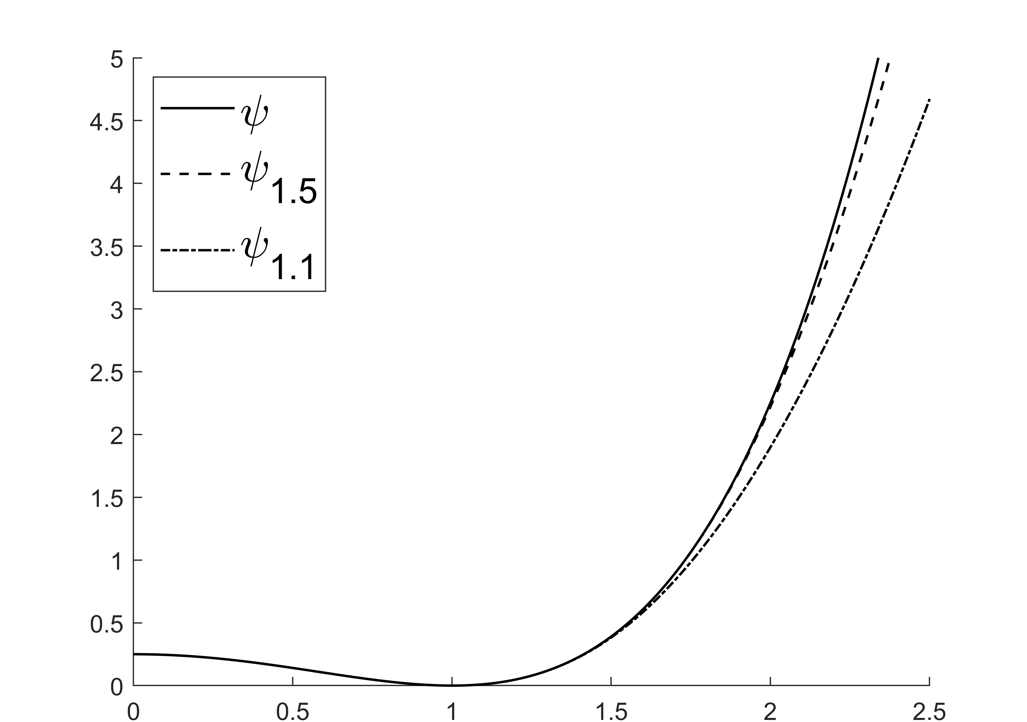
Figure 1: Plot of the double-well potential $\psi$ and
the approximate potentials $\psi_{1.5}$ and $\psi_{1.1}$.

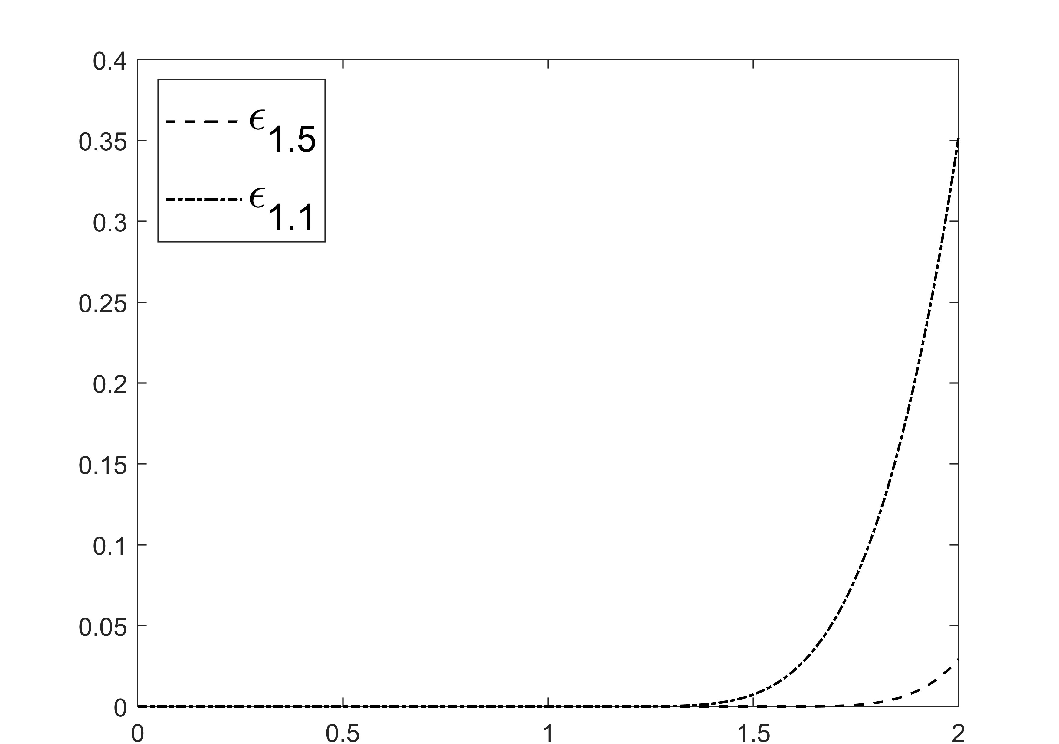
Figure 2: Plot of the error $\epsilon_{1.5}:=\psi-\psi_{1.5}$
and $\epsilon_{1.1}:=\psi-\psi_{1.1}$.

We will now present the proof of our theorem:

• To prove global optimality of the control ${\bar{u}}$, we intend to show that $J(u)-J({\bar{u}})\geq 0$ for all $u\in\mathbb{U}\setminus\{{\bar{u}}\}$. The proof is divided into three steps.

Step 1:

Let $u\in\mathbb{U}$ be arbitrary. Recall that

$$\big{(}\kappa{\bar{u}}\,{,}\,u-{\bar{u}}\big{)}_{L^{2}(L^{2})}\geq-\big{(}\phi_{\bar{u}}\,\mathds{h}(\varphi_{\bar{u}})\,{,}\,u-{\bar{u}}\big{)}_{L^{2}(L^{2})}$$

due to the variational inequality (96). Then, by a straightforward computation, we obtain that

$$J(u)-J({\bar{u}}) \geq\frac{\upalpha_{0}}{2}\lVert\varphi_{u}(T)-\varphi_{\bar{u}}(T)\rVert_{L^{2}}^{2}+\frac{\upalpha_{1}}{2}\lVert\varphi_{u}-\varphi_{\bar{u}}\rVert_{L^{2}(L^{2})}^{2}+\frac{\kappa}{2}\lVert u-{\bar{u}}\rVert_{L^{2}(L^{2})}^{2}+\mathcal{R},$$ (111)

where

$$\mathcal{R}:=\alpha_{0}\big{(}\varphi_{\bar{u}}(T)-\varphi_{f}\,{,}\,\varphi_{u}(T)-\varphi_{\bar{u}}(T)\big{)}_{L^{2}}+\alpha_{1}\big{(}\varphi_{\bar{u}}-\varphi_{d}\,{,}\,\varphi_{u}-\varphi_{\bar{u}}\big{)}_{L^{2}(L^{2})}-\big{(}\phi_{\bar{u}}\,\mathds{h}(\varphi_{\bar{u}})\,{,}\,u-{\bar{u}}\big{)}_{L^{2}(L^{2})}.$$

Our aim is to show that

$$|\mathcal{R}|\leq\frac{\upalpha_{1}}{2}\lVert\varphi_{u}-\varphi_{\bar{u}}\rVert_{L^{2}(L^{2})}^{2}+\frac{\kappa}{2}\lVert u-{\bar{u}}\rVert_{L^{2}(L^{2})}^{2}\quad\text{for all}\;u\in\mathbb{U}\setminus\{{\bar{u}}\}$$ (112)

if condition (G1) or condition (G2) is fulfilled. Then (111) yields $J(u)\geq J({\bar{u}})$ and global optimality of ${\bar{u}}$ directly follows.

Step 2:

The idea is to express the remainder $\mathcal{R}$ by the adjoint variables. For brevity, we write

$$({\tilde{\varphi}},{\tilde{\mu}},{\tilde{\sigma}},{\tilde{\mathbf{v}}},{\tilde{p}}):=(\varphi_{u},\mu_{u},\sigma_{u},\mathbf{v}_{u},p_{u})-(\varphi_{\bar{u}},\mu_{\bar{u}},\sigma_{\bar{u}},\mathbf{v}_{\bar{u}},p_{\bar{u}}).$$

This means that $({\tilde{\varphi}},{\tilde{\mu}},{\tilde{\sigma}},{\tilde{\mathbf{v}}},{\tilde{p}})$ is a solution of (20). In the following, the strategy is to test the equations of the system (20) with the adjoint variables. Testing (20c) with $\phi_{\bar{u}}$ and integration by parts with respect to $t$ yields

$$0 =\int_{\Omega_{T}}\Big{[}\partial_{t}{\tilde{\varphi}}+\textnormal{div}(\varphi_{u}{\tilde{\mathbf{v}}})+\textnormal{div}({\tilde{\varphi}}\mathbf{v}_{\bar{u}})-m\Delta{\tilde{\mu}}-P{\tilde{\sigma}}\mathds{h}(\varphi_{u})-(P\sigma_{\bar{u}}-A)\big{(}\mathds{h}(\varphi_{u})-\mathds{h}(\varphi_{\bar{u}})\big{)}$$

$$\qquad\qquad+\big{(}u\mathds{h}(\varphi_{u})-{\bar{u}}\mathds{h}(\varphi_{\bar{u}})\big{)}\Big{]}\;\phi_{\bar{u}}\;\mathrm{d}(x,t)$$

$$=\int_{\Omega_{T}}\textnormal{div}(\varphi_{u}{\tilde{\mathbf{v}}})\phi_{\bar{u}}+\textnormal{div}({\tilde{\varphi}}\mathbf{v}_{\bar{u}})\phi_{\bar{u}}-m\Delta{\tilde{\mu}}\,\phi_{\bar{u}}-P{\tilde{\sigma}}\mathds{h}(\varphi_{u})\phi_{\bar{u}}-(P\sigma_{\bar{u}}-A)\big{(}\mathds{h}(\varphi_{u})-\mathds{h}(\varphi_{\bar{u}})\big{)}\phi_{\bar{u}}\;\mathrm{d}(x,t)$$

$$\quad+\int_{\Omega_{T}}u\mathds{h}(\varphi_{u})\phi_{\bar{u}}-{\bar{u}}\mathds{h}(\varphi_{\bar{u}})\phi_{\bar{u}}\;\mathrm{d}(x,t)+\int_{\Omega}{\tilde{\varphi}}(T)\,\phi_{\bar{u}}(T)\;\mathrm{d}x-\int_{0}^{T}\langle\partial_{t}\phi_{\bar{u}}\,{,}\,{\tilde{\varphi}}\rangle_{H^{1}}\;\mathrm{d}t.$$

Now, the term $\langle\partial_{t}\phi_{\bar{u}}\,{,}\,{\tilde{\varphi}}\rangle_{H^{1}}$ can be expressed by (81) with test function ${\tilde{\phi}}={\tilde{\varphi}}$. We obtain that

$$0 =\int_{\Omega_{T}}\textnormal{div}(\varphi_{u}{\tilde{\mathbf{v}}})\phi_{\bar{u}}-P{\tilde{\sigma}}\mathds{h}(\varphi_{u})\phi_{\bar{u}}-(P\sigma_{\bar{u}}-A)\big{(}\mathds{h}(\varphi_{u})-\mathds{h}(\varphi_{\bar{u}})\big{)}\phi_{\bar{u}}+u\mathds{h}(\varphi_{u})\phi_{\bar{u}}-{\bar{u}}\mathds{h}(\varphi_{\bar{u}})\phi_{\bar{u}}\;\mathrm{d}(x,t)$$

$$\quad+\int_{\Omega_{T}}-m\Delta{\tilde{\mu}}\,\phi_{\bar{u}}+(P\sigma_{\bar{u}}-A-{\bar{u}})\mathds{h}^{\prime}(\varphi_{\bar{u}})\phi_{\bar{u}}{\tilde{\varphi}}+\mathds{h}^{\prime}(\varphi_{\bar{u}})\sigma_{\bar{u}}\rho_{\bar{u}}{\tilde{\varphi}}+\psi^{\prime\prime}(\varphi_{\bar{u}})\tau_{\bar{u}}{\tilde{\varphi}}-(P\sigma_{\bar{u}}-A)\mathds{h}^{\prime}(\varphi_{\bar{u}})q_{\bar{u}}{\tilde{\varphi}}\;\mathrm{d}(x,t)$$

$$\quad+\int_{\Omega_{T}}\upalpha_{1}(\varphi_{\bar{u}}-\varphi_{d}){\tilde{\varphi}}+(\mu_{\bar{u}}+\chi\sigma_{\bar{u}})\mathbf{w}_{\bar{u}}\cdot\nabla{\tilde{\varphi}}+\nabla\tau_{\bar{u}}\cdot\nabla{\tilde{\varphi}}\;\mathrm{d}(x,t)+\int_{\Omega}{\tilde{\varphi}}(T)\,\phi_{\bar{u}}(T)\;\mathrm{d}x.$$ (113)

Furthermore, testing (20b) with $\mathbf{w}_{\bar{u}}$ yields

$$0 =\int_{\Omega_{T}}-\textnormal{div}\big{(}T({\tilde{\mathbf{v}}},{\tilde{p}})\big{)}\cdot\mathbf{w}_{\bar{u}}+\nu{\tilde{\mathbf{v}}}\cdot\mathbf{w}_{\bar{u}}-({\tilde{\mu}}+\chi{\tilde{\sigma}})\nabla\varphi_{u}\cdot\mathbf{w}_{\bar{u}}-(\mu_{\bar{u}}+\chi\sigma_{\bar{u}})\nabla{\tilde{\varphi}}\cdot\mathbf{w}_{\bar{u}}\;\mathrm{d}(x,t)$$

$$=\int_{\Omega_{T}}2\eta{\mathbf{D}}\mathbf{w}_{\bar{u}}:\nabla{\tilde{\mathbf{v}}}+\nu{\tilde{\mathbf{v}}}\cdot\mathbf{w}_{\bar{u}}-({\tilde{\mu}}+\chi{\tilde{\sigma}})\nabla\varphi_{u}\cdot\mathbf{w}_{\bar{u}}-(\mu_{\bar{u}}+\chi\sigma_{\bar{u}})\nabla{\tilde{\varphi}}\cdot\mathbf{w}_{\bar{u}}\;\mathrm{d}(x,t)$$

due to the definition of $T({\tilde{\mathbf{v}}},{\tilde{p}})$ and the fact that $\textnormal{div}(\mathbf{w}_{\bar{u}})=0$. The term $2\eta{\mathbf{D}}\mathbf{w}_{\bar{u}}:\nabla{\tilde{\mathbf{v}}}$ can be expressed by choosing ${\tilde{\mathbf{w}}}={\tilde{\mathbf{v}}}$ in (80). Thus,

$$0 =\int_{\Omega_{T}}\textnormal{div}({\tilde{\mathbf{v}}})q_{\bar{u}}-\phi_{\bar{u}}\nabla\varphi_{u}\cdot{\tilde{\mathbf{v}}}-\phi_{\bar{u}}\varphi_{u}\textnormal{div}({\tilde{\mathbf{v}}})-({\tilde{\mu}}+\chi{\tilde{\sigma}})\nabla\varphi_{u}\cdot\mathbf{w}_{\bar{u}}-(\mu_{\bar{u}}+\chi\sigma_{\bar{u}})\nabla{\tilde{\varphi}}\cdot\mathbf{w}_{\bar{u}}\;\mathrm{d}(x,t).$$ (114)

Proceeding similarly with the other subequations of (20) gives

$$0 =\int_{\Omega_{T}}\nabla\varphi_{\bar{u}}\cdot\mathbf{w}_{\bar{u}}\,{\tilde{\mu}}+m\Delta{\tilde{\mu}}\,\phi_{\bar{u}}-\nabla{\tilde{\varphi}}\cdot\nabla\tau_{\bar{u}}-\big{(}\psi^{\prime}(\varphi_{u})-\psi^{\prime}(\varphi_{\bar{u}})\big{)}\tau_{\bar{u}}+\chi{\tilde{\sigma}}\tau_{\bar{u}}\;\mathrm{d}(x,t),$$ (115)

$$0 =\int_{\Omega_{T}}-\textnormal{div}({\tilde{\mathbf{v}}})q_{\bar{u}}+P{\tilde{\sigma}}\mathds{h}(\varphi_{u})q_{\bar{u}}+(P\sigma_{u}-A)\big{(}\mathds{h}(\varphi_{u})-\mathds{h}(\varphi_{\bar{u}})\big{)}q_{\bar{u}}\;\mathrm{d}(x,t),$$ (116)

$$0 =\int_{\Omega_{T}}-\chi\tau_{\bar{u}}{\tilde{\sigma}}+P{\tilde{\sigma}}\mathds{h}(\varphi_{u})\phi_{\bar{u}}+\chi{\tilde{\sigma}}\nabla\varphi_{u}\cdot\mathbf{w}_{\bar{u}}-P{\tilde{\sigma}}\mathds{h}(\varphi_{u})q_{\bar{u}}-\sigma_{\bar{u}}\rho_{\bar{u}}\big{(}\mathds{h}(\varphi_{u})-\mathds{h}(\varphi_{\bar{u}})\big{)}\;\mathrm{d}(x,t).$$ (117)

Adding up (5.4)-(117), we ascertain that a large number of terms cancels out. We end up with

$$0 =\int_{\Omega}\phi_{\bar{u}}(T){\tilde{\varphi}}(T)\;\mathrm{d}x+\upalpha_{1}\int_{\Omega_{T}}(\varphi_{\bar{u}}-\varphi_{d}){\tilde{\varphi}}\;\mathrm{d}(x,t)+\int_{\Omega_{T}}(u-{\bar{u}})\mathds{h}(\varphi_{u})\phi_{\bar{u}}\;\mathrm{d}(x,t)$$

$$\quad+\int_{\Omega_{T}}(P\sigma_{\bar{u}}-A)\big{(}\mathds{h}(\varphi_{u})-\mathds{h}(\varphi_{\bar{u}})-\mathds{h}^{\prime}(\varphi_{u}){\tilde{\varphi}}\big{)}(q_{\bar{u}}-\phi_{\bar{u}})\;\mathrm{d}(x,t)$$

$$\quad+\int_{\Omega_{T}}\sigma_{\bar{u}}\rho_{\bar{u}}\big{(}\mathds{h}(\varphi_{u})-\mathds{h}(\varphi_{\bar{u}})-\mathds{h}^{\prime}(\varphi_{u}){\tilde{\varphi}}\big{)}\;\mathrm{d}(x,t)$$

$$\quad-\int_{\Omega_{T}}\big{(}\psi^{\prime}(\varphi_{u})-\psi^{\prime}(\varphi_{\bar{u}})-\psi^{\prime\prime}(\varphi_{\bar{u}}){\tilde{\varphi}}\big{)}\tau_{\bar{u}}\;\mathrm{d}(x,t)$$

$$\quad+\int_{\Omega_{T}}{\bar{u}}\big{(}\mathds{h}(\varphi_{u})-\mathds{h}(\varphi_{\bar{u}})-\mathds{h}^{\prime}(\varphi_{\bar{u}}){\tilde{\varphi}}\big{)}\phi_{\bar{u}}+(u-{\bar{u}})\big{(}\mathds{h}(\varphi_{u})-\mathds{h}(\varphi_{\bar{u}})\big{)}\phi_{\bar{u}}\;\mathrm{d}(x,t).$$ (118)

Since $\phi_{\bar{u}}(T)=\upalpha(\varphi_{\bar{u}}(T)-\varphi_{f})$, the first three terms on the right-hand side of (5.4) are equal to $\mathcal{R}$. Moreover, using Taylor expansion, we can find $\zeta,\xi,\theta\in[0,1]$ such that

$$\mathds{h}(\varphi_{u})-\mathds{h}(\varphi_{\bar{u}}) =\mathds{h}^{\prime}(\varphi_{\zeta}){\tilde{\varphi}}^{2} \quad\text{with}\quad\varphi_{\zeta}=\varphi_{\bar{u}}+\zeta(\varphi_{u}-\varphi_{\bar{u}}),$$

$$\mathds{h}(\varphi_{u})-\mathds{h}(\varphi_{\bar{u}})-\mathds{h}^{\prime}(\varphi_{u}){\tilde{\varphi}} =\mathds{h}^{\prime\prime}(\varphi_{\xi}){\tilde{\varphi}}^{2} \quad\text{with}\quad\varphi_{\xi}=\varphi_{\bar{u}}+\xi(\varphi_{u}-\varphi_{\bar{u}}),$$

$$\psi^{\prime}(\varphi_{u})-\psi^{\prime}(\varphi_{\bar{u}})-\psi^{\prime\prime}(\varphi_{u}){\tilde{\varphi}} =\psi^{\prime\prime\prime}(\varphi_{\theta}){\tilde{\varphi}}^{2} \quad\text{with}\quad\varphi_{\theta}=\varphi_{\bar{u}}+\theta(\varphi_{u}-\varphi_{\bar{u}}).$$

Hence, it follows that

$$\mathcal{R} =\int_{\Omega_{T}}\Big{[}(P\sigma_{\bar{u}}-A)(\phi_{\bar{u}}-q_{\bar{u}})-\sigma_{\bar{u}}\rho_{\bar{u}}-{\bar{u}}\phi_{\bar{u}}\Big{]}\mathds{h}^{\prime\prime}(\varphi_{\xi}){\tilde{\varphi}}^{2}\;\mathrm{d}(x,t)$$

$$\quad+\int_{\Omega_{T}}\tau_{\bar{u}}\psi^{\prime\prime\prime}(\varphi_{\theta}){\tilde{\varphi}}^{2}\;\mathrm{d}(x,t)+\int_{\Omega_{T}}(u-{\bar{u}})\phi_{\bar{u}}\mathds{h}^{\prime}(\varphi_{\zeta}){\tilde{\varphi}}\;\mathrm{d}(x,t).$$ (119)

Step 3:

Now, we will use (5.4) to prove estimates in the fashion of (112). A simple computation gives

$$|\mathcal{R}| \leq\Big{[}\big{\|}(P\sigma_{\bar{u}}-A)(\phi_{\bar{u}}-q_{\bar{u}})-\sigma_{\bar{u}}\rho_{\bar{u}}-{\bar{u}}\phi_{\bar{u}}\big{\|}_{1}\lVert\mathds{h}^{\prime\prime}\rVert_{L^{\infty}(\mathbb{R})}\,L_{1}^{2}$$

$$\qquad+\lVert\tau_{\bar{u}}\rVert_{1}\,\lVert\psi^{\prime\prime\prime}\rVert_{L^{\infty}([-r,r])}\,L_{1}^{2}+\lVert\phi_{\bar{u}}\rVert_{2}\lVert\mathds{h}^{\prime}\rVert_{L^{\infty}(\mathbb{R})}\,L_{1}\Big{]}\,\lVert u-{\bar{u}}\rVert_{2}^{2},$$ (120)

since $\lVert\varphi_{\theta}\rVert_{\infty}\leq r$. Furthermore, using Young’s inequality with $\theta$, the remainder $\mathcal{R}$ can also be bounded by

$$|\mathcal{R}| \leq\Big{[}\big{\|}(P\sigma_{\bar{u}}-A)(\phi_{\bar{u}}-q_{\bar{u}})-\sigma_{\bar{u}}\rho_{\bar{u}}-{\bar{u}}\phi_{\bar{u}}\big{\|}_{\infty}\lVert\mathds{h}^{\prime\prime}\rVert_{L^{\infty}(\mathbb{R})}$$

$$\qquad\quad+\lVert\tau_{\bar{u}}\rVert_{\infty}\lVert\psi^{\prime\prime\prime}\rVert_{L^{\infty}([-r,r])}+\theta\lVert\phi_{\bar{u}}\rVert_{\infty}^{2}\lVert\mathds{h}^{\prime}\rVert_{L^{\infty}(\mathbb{R})}^{2}\Big{]}\lVert{\tilde{\varphi}}\rVert_{L^{2}(L^{2})}^{2}$$

$$\qquad+\frac{1}{4\theta}\lVert\phi_{\bar{u}}\rVert_{\infty}^{2}\lVert\mathds{h}^{\prime}\rVert_{L^{\infty}(\mathbb{R})}^{2}\lVert u-{\bar{u}}\rVert_{L^{2}(L^{2})}^{2}.$$ (121)

Hence, if condition (G1) or condition (G2) is satisfied, we can use (5.4) or (5.4) to conclude that

$$|\mathcal{R}| \leq\frac{\upalpha_{1}}{2}\lVert{\tilde{\varphi}}\rVert_{L^{2}(L^{2})}^{2}+\frac{\kappa}{2}\lVert u-{\bar{u}}\rVert_{L^{2}(L^{2})}^{2}$$ (122)

and inequality (111) implies that ${\bar{u}}$ is a globally optimal control. If, in addition, either condition (U1) or (U2) is satisfied, it even holds that

$$|\mathcal{R}| <\frac{\upalpha_{1}}{2}\lVert{\tilde{\varphi}}\rVert_{L^{2}(L^{2})}^{2}+\frac{\kappa}{2}\lVert u-{\bar{u}}\rVert_{L^{2}(L^{2})}^{2}.$$ (123)

Then (111) implies that

$$J(u)>J({\bar{u}})\quad\text{for all}\;u\in\mathbb{U}\setminus\{{\bar{u}}\}$$

and uniqueness of the globally optimal control ${\bar{u}}$ follows. ∎

5.5 Uniqueness of the optimal control on small time intervals

Finally, we present a condition on $T$ which ensures uniqueness of the optimal control. A similar result was established, e.g., in [37, 38]. The idea behind the approach is as follows: If we choose the final time $T$ sufficiently small, the state equation will differ only slightly from its linearization. In the case $\kappa>0$, a linearized state equation would produce a strictly convex cost functional and the corresponding optimal control would be unique. If $T$ is small enough, we can expect that this property transfers to our problem. On the other hand, if the parameter $\kappa$ is large, the strictly convex part of the cost functional $J$ will be more dominant. Thus, it is not surprising that the size of the time interval on which the optimal control is unique will also depend on $\kappa$.
In our theorem, we use the following notation: For any $p\in[1,6]$, let $c_{\Omega}(p)\geq 0$ denote a constant for which Sobolev’s inequality

$$\lVert v\rVert_{L^{p}(\Omega)}\leq c_{\Omega}(p)\,\lVert v\rVert_{H^{1}(\Omega)},\quad\text{for all}\;v\in H^{1}(\Omega),$$

is satisfied.

Theorem 31.

Suppose that $\kappa>0$ and let ${\bar{u}}\in\mathbb{U}$ be a locally optimal control of problem (94). Let $p,q\in[3,6]$ with $\frac{1}{p}+\frac{1}{q}=\frac{1}{2}$ be arbitrary.
Moreover, we assume that

$$T<\left(\frac{\sqrt{3}\,\kappa}{2\big{(}L_{3}+\sqrt{2}L_{1}c_{\Omega}(p)\,c_{\Omega}(q)\|\phi_{\bar{u}}\|_{L^{\infty}(H^{1})}\,\|\mathds{h}^{\prime}\|_{L^{\infty}(\mathbb{R})}\big{)}}\right)^{4/3}.$$ (124)

Then, ${\bar{u}}$ is the unique locally optimal control.

• Let us assume that there exists another locally optimal control $u$. Then, it holds that

  $$\|\varphi_{u}(t)-\varphi_{\bar{u}}(t)\|_{L^{2}}^{2}\leq 2\int_{0}^{t}\|\partial_{s}\varphi_{u}(s)-\partial_{s}\varphi_{\bar{u}}(s)\|_{L^{2}}\,\|\varphi_{u}(s)-\varphi_{\bar{u}}(s)\|_{L^{2}}\;\mathrm{d}s$$

  $$\quad\leq 2\sqrt{t}\,\|\varphi_{u}-\varphi_{\bar{u}}\|_{H^{1}(L^{2})}\,\|\varphi_{u}-\varphi_{\bar{u}}\|_{L^{\infty}(L^{2})}\leq 2L_{1}^{2}\sqrt{t}\,\|u-{\bar{u}}\|_{L^{2}(L^{2})}^{2}.$$

  Using integration by parts, we also obtain the estimate

  $$\|\nabla\varphi_{u}(t)-\nabla\varphi_{\bar{u}}(t)\|_{L^{2}}^{2}\leq 2\int_{0}^{t}\|\partial_{s}\varphi_{u}(s)-\partial_{s}\varphi_{\bar{u}}(s)\|_{L^{2}}\,\|\Delta\varphi_{u}(s)-\Delta\varphi_{\bar{u}}(s)\|_{L^{2}}\;\mathrm{d}s$$

  $$\quad\leq 2\sqrt{t}\,\|\varphi_{u}-\varphi_{\bar{u}}\|_{H^{1}(L^{2})}\,\|\varphi_{u}-\varphi_{\bar{u}}\|_{L^{\infty}(H^{2})}\leq 2L_{1}^{2}\sqrt{t}\,\|u-{\bar{u}}\|_{L^{2}(L^{2})}^{2}.$$

  Consequently, we have

  $$\|\varphi_{u}-\varphi_{\bar{u}}\|_{L^{2}(H^{1})}\leq\frac{2\sqrt{2}}{\sqrt{3}}\,L_{1}\,T^{3/4}\,\|u-{\bar{u}}\|_{L^{2}(L^{2})}.$$ (125)

  In the same fashion, we derive the estimate

  $$\|\phi_{u}(t)-\phi_{\bar{u}}(t)\|_{L^{2}}^{2}=2\int_{t}^{T}\langle\partial_{s}\phi_{u}(s)-\partial_{s}\phi_{\bar{u}}(s)\,{,}\,\phi_{u}(s)-\phi_{\bar{u}}(s)\rangle_{H^{1}}\;\mathrm{d}s$$

  $$\quad\leq 2\sqrt{T-t}\,\|\phi_{u}-\phi_{\bar{u}}\|_{H^{1}((H^{1})^{*})}\,\|\phi_{u}-\phi_{\bar{u}}\|_{L^{\infty}(H^{1})}\leq 2L_{3}^{2}\sqrt{T-t}\,\|u-{\bar{u}}\|_{L^{2}(L^{2})}^{2}$$

  and thus,

  $$\|\phi_{u}-\phi_{\bar{u}}\|_{L^{2}(L^{2})}\leq\frac{2}{\sqrt{3}}\,L_{3}\,T^{3/4}\,\|u-{\bar{u}}\|_{L^{2}(L^{2})}.$$ (126)

  Furthermore, we know from Corollary 24 that both $u$ and ${\bar{u}}$ satisfy the projection formula (97). A straightforward computation yields

  $$|u(x,t)-{\bar{u}}(x,t)|\leq\frac{1}{\kappa}\|\mathds{h}\|_{L^{\infty}(\mathbb{R})}|\phi_{u}(x,t)-\phi_{\bar{u}}(x,t)|+|\phi_{\bar{u}}(x,t)|\,\|\mathds{h}^{\prime}\|_{L^{\infty}(\mathbb{R})}|\varphi_{u}(x,t)-\varphi_{\bar{u}}(x,t)|$$

  for almost all $(x,t)\in{\Omega_{T}}$. Recall that $\|\mathds{h}\|_{L^{\infty}(\mathbb{R})}\leq 1$. Hence, using (125) and (126), we conclude that

  $$\lVert u-{\bar{u}}\rVert_{L^{2}(L^{2})} \leq\frac{1}{\kappa}\|\phi_{u}-\phi_{\bar{u}}\|_{L^{2}(L^{2})}+\frac{1}{\kappa}\|\phi_{\bar{u}}\|_{L^{\infty}(L^{p})}\,\|\mathds{h}^{\prime}\|_{L^{\infty}(\mathbb{R})}\,\|\varphi_{u}-\varphi_{\bar{u}}\|_{L^{2}(L^{q})}$$

  $$\leq\frac{1}{\kappa}\|\phi_{u}-\phi_{\bar{u}}\|_{L^{2}(L^{2})}+\frac{1}{\kappa}c_{\Omega}(p)\|\phi_{\bar{u}}\|_{L^{\infty}(H^{1})}\,\|\mathds{h}^{\prime}\|_{L^{\infty}(\mathbb{R})}\,c_{\Omega}(q)\|\varphi_{u}-\varphi_{\bar{u}}\|_{L^{2}(H^{1})}$$

  $$\leq\frac{2}{\sqrt{3}\kappa}\;T^{3/4}\;\Big{(}L_{3}+\sqrt{2}L_{1}c_{\Omega}(p)\,c_{\Omega}(q)\|\phi_{\bar{u}}\|_{L^{\infty}(H^{1})}\,\|\mathds{h}^{\prime}\|_{L^{\infty}(\mathbb{R})}\Big{)}\,\|u-{\bar{u}}\|_{L^{2}(L^{2})}.$$

  However, if (124) is satisfied, we have

  $$\frac{2}{\sqrt{3}\kappa}\;T^{3/4}\;\Big{(}L_{3}+\sqrt{2}L_{1}c_{\Omega}(p)\,c_{\Omega}(q)\|\phi_{\bar{u}}\|_{L^{\infty}(H^{1})}\,\|\mathds{h}^{\prime}\|_{L^{\infty}(\mathbb{R})}\Big{)}<1.$$

  Therefore, the above inequality can hold true only if $\|u-{\bar{u}}\|_{L^{2}(L^{2})}=0$ which means uniqueness of the locally optimal control. ∎

Corollary 32.

Suppose that $T>0$ and $\kappa>0$ satisfy the assumption (124) of Theorem 31. Then, there exists a unique globally optimal control ${\bar{u}}$ of problem (94).
In this case, each of the equivalent necessary optimality conditions (96) and (97) is a sufficient condition for global optimality.

• Theorem 22 ensures the existence of at least one globally optimal control ${\bar{u}}\in\mathbb{U}$. Of course, ${\bar{u}}$ is also locally optimal. Hence, since assumption (124) holds, Theorem 31 implies that ${\bar{u}}$ is the unique locally optimal control. It follows immediately that ${\bar{u}}$ is the unique globally optimal control.
  Moreover, ${\bar{u}}$ satisfies the equivalent necessary optimality conditions (96) and (97). Because of Theorem 31 it is also the only control satisfying these conditions. Hence, (96) (or (97), respectively) is a sufficent condition for global optimality. ∎

References

- [1] A. Agosti, C. Cattaneo, C. Giverso, D. Ambrosi, and P. Ciarletta. A computational framework for the personalized clinical treatment of glioblastoma multiforme. ZAMM - Journal of Applied Mathematics and Mechanics / Zeitschrift für Angewandte Mathematik und Mechanik, 2018.
- [2] A. Ahmad Ali, K. Deckelnick, and M. Hinze. Global minima for semilinear optimal control problems. Comput. Optim. Appl., 65(1):261–288, 2016.
- [3] A. Ahmad Ali, K. Deckelnick, and M. Hinze. Global minima for optimal control of the obstacle problem. ESAIM Control Optim. Calc. Var., https://doi.org/10.1051/cocv/2019039, 2019.
- [4] E.L. Bearer, J.S. Lowengrub, H.B. Frieboes, Y.L. Chuang, F. Jin, S.M. Wise, M. Ferrari, and V. Agus, D.B.and Cristini. Multiparameter computational modeling of tumor invasion. Cancer Research, 69(10):4493–4501, 2009.
- [5] C. Benosman, B. Aïnseba, and A. Ducrot. Optimization of Cytostatic Leukemia Therapy in an Advection–Reaction–Diffusion Model. Journal of Optimization Theory and Applications, 167(1):296–325, 2015.
- [6] T. Biswas, S. Dharmatti, and M.T. Mohan. Pontryagin’s maximum principle for optimal control of the nonlocal Cahn–Hilliard–Navier–Stokes systems in two dimensions. ArXiv e-prints: arXiv:1802.08413, 2018.
- [7] J. F. Blowey and C. M. Elliott. The Cahn–Hilliard gradient theory for phase separation with nonsmooth free energy. I. Mathematical analysis. European J. Appl. Math., 2(3):233–280, 1991.
- [8] H. Byrne and M. Chaplain. Free boundary value problems associated with the growth and development of multicellular spheroids. Euro. Jnl. of Applied Mathematics, 8:639–658, 1997.
- [9] E. Casas, J.C. de los Reyes, and F. Tröltzsch. Sufficient second-order optimality conditions for semilinear control problems with pointwise state constraints. SIAM J. Optim., 19(2):616–643, 2008.
- [10] C. Cavaterra, E. Rocca, and H. Wu. Long-time dynamics and optimal control of a diffuse interface model for tumor growth. Appl. Math. Optim., 2019.
- [11] M. Chaplain. Avascular growth, angiogenesis and vascular growth in solid tumours: The mathematical modelling of the stages of tumour development. Mathematical and Computer Modelling, 23(6):47–87, 1996.
- [12] P. Colli, M.H. Farshbaf-Shaker, G. Gilardi, and J. Sprekels. Optimal boundary control of a viscous Cahn–Hilliard system with dynamic boundary condition and double obstacle potentials. SIAM J. Control Optim., 53(4):2696–2721, 2015.
- [13] P. Colli, G. Gilardi, E. Rocca, and J. Sprekels. Optimal distributed control of a diffuse interface model of tumor growth. Nonlinearity, 30(6):2518–2546, 2017.
- [14] P. Colli, G. Gilardi, and J. Sprekels. Optimal velocity control of a viscous Cahn–Hilliard system with convection and dynamic boundary conditions. SIAM J. Control Optim., 56(3):1665–1691, 2018.
- [15] V. Cristini, X. Li, J. S. Lowengrub, and S. M. Wise. Nonlinear simulations of solid tumor growth using a mixture model: invasion and branching. J. Math. Biol., 58(4-5):723–763, 2009.
- [16] M. Ebenbeck and H. Garcke. Analysis of a Cahn–Hilliard–Brinkman model for tumour growth with chemotaxis. J. Differential Equations, 266(9):5998–6036, 2018.
- [17] M. Ebenbeck and H. Garcke. On a Cahn–Hilliard–Brinkman model for tumor growth and its singular limits. SIAM J. Math. Anal., 51(3):1868–1912, 2019.
- [18] M. Ebenbeck and P. Knopf. Optimal medication for tumors modeled by a Cahn–Hilliard–Brinkman equation. Calc. Var. Partial Differential Equations, 58(4):Art. 131, 31, 2019.
- [19] S. J. Franks and J. R. King. Interactions between a uniformly proliferating tumour and its surroundings: uniform material properties. Math. Med. Biol., 20(1):47–89, 2003.
- [20] S. J. Franks and J. R. King. Interactions between a uniformly proliferating tumour and its surroundings: stability analysis for variable material properties. Internat. J. Engrg. Sci., 47(11-12):1182–1192, 2009.
- [21] H.B. Frieboes, J. Lowengrub, S. Wise, X. Zheng, P. Macklin, E. Bearer, and V. Cristini. Computer simulation of glioma growth and morphology. NeuroImage, 37 Suppl 1:59–70, 02 2007.
- [22] A. Friedman. A free boundary problem for a coupled system of elliptic, hyperbolic, and Stokes equations modeling tumor growth. Interfaces Free Bound., 8(2):247–261, 2006.
- [23] S. Frigeri, M. Grasselli, and E. Rocca. On a diffuse interface model of tumour growth. European J. Appl. Math., 26(2):215–243, 2015.
- [24] S. Frigeri, E. Rocca, and J. Sprekels. Optimal distributed control of a nonlocal Cahn–Hilliard/Navier–Stokes system in two dimensions. SIAM J. Control Optim., 54(1):221–250, 2016.
- [25] Y.C. Fung. Biomechanics: Mechanical Properties of Living Tissues. Springer, New York, 1993.
- [26] H. Garcke and K. F. Lam. Well-posedness of a Cahn-Hilliard system modelling tumour growth with chemotaxis and active transport. European J. Appl. Math., 28(2):284–316, 2017.
- [27] H. Garcke, K. F. Lam, and E. Rocca. Optimal control of treatment time in a diffuse interface model of tumor growth. Appl. Math. Optim., 78(3):495–544, 2018.
- [28] H. Garcke, K.F. Lam, R. Nürnberg, and E. Sitka. A multiphase Cahn–Hilliard–Darcy model for tumour growth with necrosis. Math. Models Methods Appl. Sci., 28(3):525–577, 2018.
- [29] H. Garcke, K.F. Lam, E. Sitka, and V. Styles. A Cahn–Hilliard–Darcy model for tumour growth with chemotaxis and active transport. Math. Models Methods Appl. Sci., 26(6):1095–1148, 2016.
- [30] H. Garcke, K.F. Lam, and V. Styles. Cahn–Hilliard inpainting with double obstacle potential. SIAM J. Imaging Sci., 11(3):2064–2089, 2018.
- [31] G. Gilardi and J. Sprekels. Asymptotic limits and optimal control for the Cahn–Hilliard system with convection and dynamic boundary conditions. Nonlinear Analysis, 178:1–31, 2019.
- [32] H. P. Greenspan. On the growth and stability of cell cultures and solid tumors. J. Theoret. Biol., 56(1):229–242, 1976.
- [33] A. Hawkins-Daarud, K. G. van der Zee, and J. T. Oden. Numerical simulation of a thermodynamically consistent four-species tumor growth model. Int. J. Numer. Methods Biomed. Eng., 28(1):3–24, 2012.
- [34] D. Hilhorst, J. Kampmann, T. N. Nguyen, and K. G. Van Der Zee. Formal asymptotic limit of a diffuse-interface tumor-growth model. Math. Models Methods Appl. Sci., 25(6):1011–1043, 2015.
- [35] M. Hintermüller and D. Wegner. Distributed optimal control of the Cahn–Hilliard system including the case of a double-obstacle homogeneous free energy density. SIAM J. Control Optim., 50(1):388–418, 2012.
- [36] C. Kahle and K.F. Lam. Parameter Identification via Optimal Control for a Cahn–Hilliard-Chemotaxis System with a Variable Mobility. Appl. Math. Optim., Mar 2018.
- [37] P. Knopf. Optimal control of a Vlasov–Poisson plasma by an external magnetic field. Calc. Var., 57(134), 2018.
- [38] P. Knopf and J. Weber. Optimal Control of a Vlasov–Poisson Plasma by Fixed Magnetic Field Coils. Appl. Math. Optim., https://doi.org/10.1007/s00245-018-9526-5, 2018.
- [39] U. Ledzewicz and H. Schättler. Multi-input optimal control problems for combined tumor anti-angiogenic and radiotherapy treatments. J. Optim. Theory Appl., 153(1):195–224, 2012.
- [40] J. T. Oden, A. Hawkins, and S. Prudhomme. General diffuse-interface theories and an approach to predictive tumor growth modeling. Math. Models Methods Appl. Sci., 20(3):477–517, 2010.
- [41] S.I. Oke, M.B. Matadi, and S.S. Xulu. Optimal Control Analysis of a Mathematical Model for Breast Cancer. Mathematical and Computational Applications, 23(2), 2018.
- [42] B. Perthame and N. Vauchelet. Incompressible limit of a mechanical model of tumour growth with viscosity. Philos. Trans. Roy. Soc. A, 373(2050):20140283, 16, 2015.
- [43] H. Schättler and U. Ledzewicz. Optimal control for mathematical models of cancer therapies, volume 42 of Interdisciplinary Applied Mathematics. Springer, New York, 2015. An application of geometric methods.
- [44] A. Signori. Optimal Distributed Control of an Extended Model of Tumor Growth with Logarithmic Potential. Appl. Math. Optim., https://doi.org/10.1007/s00245-018-9538-1, 2018.
- [45] A. Signori. Optimal treatment for a phase field system of Cahn–Hilliard type modeling tumor growth by asymptotic scheme. Mathematical Control & Related Fields, https://doi.org/10.3934/mcrf.2019040, 2019.
- [46] A. Signori. Optimality conditions for an extended tumor growth model with double obstacle potential via deep quench approach. Evolution Equations & Control Theory, https://doi.org/10.3934/eect.2020003, 2019.
- [47] J. Simon. Compact sets in the space . Annali di Matematica Pura ed Applicata, 146(1):65–96, 1986.
- [48] J. Sprekels and H. Wu. Optimal Distributed Control of a Cahn–Hilliard–Darcy System with Mass Sources. Appl. Math. Optim., 2019.
- [49] G.W. Swan. Role of optimal control theory in cancer chemotherapy. Mathematical Biosciences, 101(2):237–284, 1990.
- [50] F. Tröltzsch. Optimal Control of Partial Differential Equations: Theory, Methods and Applications, Graduate Studies in Mathematics (Vol. 112). Amer. Math. Soc., 2010.
- [51] X. Zhao and C. Liu. Optimal control of the convective Cahn–Hilliard equation. Appl. Anal., 92(5):1028–1045, 2013.
- [52] X. Zhao and C. Liu. Optimal control for the convective Cahn–Hilliard equation in 2D case. Appl. Math. Optim., 70(1):61–82, 2014.
- [53] X. Zheng, S. M. Wise, and V. Cristini. Nonlinear simulation of tumor necrosis, neo-vascularization and tissue invasion via an adaptive finite-element/level-set method. Bull. Math. Biol., 67(2):211–259, 2005.