A block-random algorithm for learning on distributed, heterogeneous data

Abstract

Most deep learning models are based on deep neural networks with multiple layers between input and output. The parameters defining these layers are initialized using random values and are “learned” from data, typically using stochastic gradient descent based algorithms. These algorithms rely on data being randomly shuffled before optimization. The randomization of the data prior to processing in batches that is formally required for stochastic gradient descent algorithm to effectively derive a useful deep learning model is expected to be prohibitively expensive for in situ model training because of the resulting data communications across the processor nodes. We show that the stochastic gradient descent (SGD) algorithm can still make useful progress if the batches are defined on a per-processor basis and processed in random order even though (i) the batches are constructed from data samples from a single class or specific flow region, and (ii) the overall data samples are heterogeneous. We present block-random gradient descent, a new algorithm that works on distributed, heterogeneous data without having to pre-shuffle. This algorithm enables in situ learning for exascale simulations. The performance of this algorithm is demonstrated on a set of benchmark classification models and the construction of a subgrid scale large eddy simulations (LES) model for turbulent channel flow using a data model similar to that which will be encountered in exascale simulation.

1 Introduction

Simulating complex physics problems while resolving all the relevant length scales is computationally expensive, requiring millions of core hours to compute a single realization. Combining direct numerical simulations (DNS) with an optimization or design cycle is infeasible, creating a need for reduced-order models. Deep learning is an increasingly popular and effective modeling technique that use many data to train a neural network for a variety of tasks [1, 2, 3, 4, 5]. These tasks range from visual object recognition and speech recognition to analyzing particle accelerator data and drug design. Recently, deep learning has been explored as a tool for creating reduced-order closure models in turbulent fluid flows [6, 7, 8].

For physics simulation, the advent of exascale computing will enable unprecedentedly high-fidelity simulations. The expectation is to derive reduced-order models for engineering and design applications from the many data generated by these simulations. Because it will be increasingly difficult to save the large amounts of data generated during the simulations for offline training, this will drive the need to change existing approaches for training deep learning models. Online or in situ training, where the model is trained during the simulation to avoid data storage, has the potential to alleviate this problem. A data parallel [9] paradigm for deep learning is a practical approach for online training. In this setting, there are two distinct computational clusters: one for the physics computations and the other for deep learning. Data will be transferred from the physics cluster to the deep learning cluster as needed by the learning algorithms.

Most deep learning models use artificial neural networks with multiple layers to capture nonlinearities. The parameters defining these layers are “learned” from data, typically using algorithms that approximate gradient descent. With the increase in the amount of available data, deterministic learning algorithms are often expensive and rarely used in practice. Stochastic gradient descent (SGD) [10, 4] and variants using “mini-batches” are commonly used algorithms for practical learning problems. The stochastic algorithms require the data to be randomly shuffled [10, 4] for optimization; however, because fully shuffling the data will be infeasible for exascale simulations because of the communication costs of moving the data between processor nodes, the data shuffling strategy necessary for SGD will need to adapt to ensure the adequate representation of the vastly differing physical processes occurring in the simulation domain. Shuffling data extracted from a single computational node will not provide sufficient randomness because correlations tend to be spatially localized. The randomization of the data prior to processing in batches that is formally required for SGD to make progress is expected to be prohibitively expensive for in situ model training. We illustrate the memory patterns in Figure 1 for the simulation of a passively advected scalar using adaptive mesh refinement (setup defined in the AMReX tutorial). The blocks of data are distributed among the different processors and are heterogeneous, with the mesh adaptivity refining areas of interest. The memory access pattern for fully shuffling the data for SGD is shown in Figure 1(c). This type of memory access is detrimental to the simulation performance because the memory access is uncoalesced, disregards data locality, and requires many global communications. A single global communication to transfer a large contiguous chunk of data from one processor is more efficient than many communications transferring smaller chunks of data from multiple processors. We show that the SGD algorithm can still make useful progress if the batches are defined on a per-processor basis and processed in random order even though (i) the batches are constructed from data samples from a single class or specific flow region, and (ii) the overall data samples are heterogeneous. In this work, we present a new block-random algorithm that works on distributed, heterogeneous data without having to pre-shuffle.

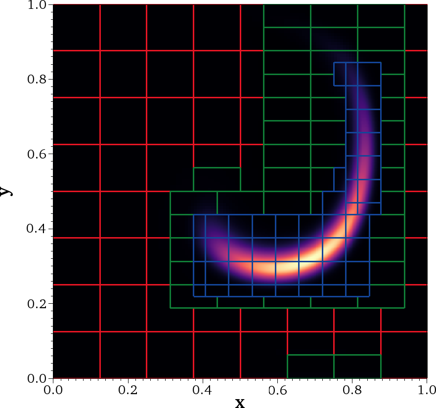
(a) Advection of a passive scalar. Red: level 0; green: level 1; blue: level 2.

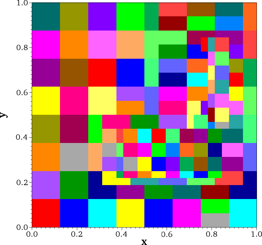
(b) Memory layout of the simulation data on the different processor ranks. Colors denote the processor ranks.

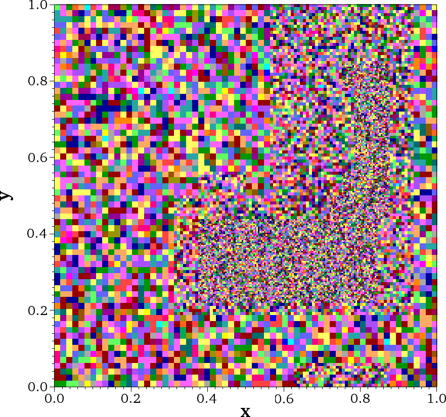
(c) Fully shuffled memory access for training with SGD. Colors denote the different batches.

Figure 1: Illustration of memory access patterns for the simulation of a vortex using adaptive mesh refinement from the AMReX tutorial.

This paper is organized as follows. In Section 2, we present the problem formulation and describe the proposed methodology for deep learning of distributed, heterogeneous data. In Section 3, we detail the architecture of the deep convolutional neural network used to perform the data recovery process for fluid flows. In Section 3.1, we evaluate our proposed method on the EMNIST data sets, a standard set of benchmark problems commonly used in deep learning. In Section 3.2, we apply our methodology to a challenge problem representative of those encountered for in situ deep learning in large scale simulations. We construct subgrid-scale (SGS) stress models for large eddy simulations using our proposed methodology and compare it to standard approaches. Finally, we present conclusions and future work in Section 4.

2 Methods

Gradient descent-based algorithms are typical optimization methods used for training deep neural networks (DNNs). Gradient descent is an algorithm to find the set of parameters $\theta$ that minimize a cost function $J(\theta)$. In the case of DNNs, the cost function is usually a normed distance between the predictions and data in a training set. The simplest form of gradient descent is:

$$\theta_{k+1}=\theta_{k}-\eta\nabla_{\theta_{k}}J(\theta_{k})$$ (1)

where $\eta$ is the learning rate, $k$ denotes subsequent iterations of the gradient descent algorithm, and $J$ is computed on the entire training data set. For very large data sets, this algorithm is very slow because it computes the cost function on the entire data set for a single update of the parameters. SGD, in contrast, performs a parameter update for each sample in the training data set. SGD and SGD variants — such as Adam [11], RMSprop [12] and Adagrad [13] — have proved to be effective ways of training DNNs. A common addition to SGD is to add “mini-batching”, where the training data are partitioned into batches of size $n_{b}$. The batching procedure is used to provide sequences of approximations of the gradient of the cost function with respect to the parameters by computing:

$$\nabla_{\theta_{k}}J(\theta_{k}|x\in b,y\in b)$$ (2)

where $b$ is a batch of training data. Mini-batching provides a better estimate of $\nabla_{\theta}J(\theta)$ by using several samples from the training set instead of only one sample. As a result, the parameter updates tend to be less noisy. It is also computationally more efficient by using vectorized computations and parallelism provided by modern architectures. In practice, the shuffled training data is divided into batches, the batches are then randomly shuffled before each pass through the training data, and each batch is used to provide gradient approximations to update the neural network model parameters. It has been shown that the SGD gradient approximations converge to the true gradient in expectation [10].

Being stochastic, however, these algorithms require the data to be randomly shuffled to converge to a minimum of the cost function. Results from Section 3.1 show how these algorithms fail to converge without shuffling when the batches have inherent bias. As described in Section 1, this shuffling operation is infeasible for online learning on exascale simulations. We propose a block-random algorithm for use in these cases where the data ordering needs to remain unchanged. The algorithm operates by swapping the order of shuffling and batching operations. This shuffling of batches appears to be sufficient for learning the parameters even when the data are highly ordered, resulting in batches with high bias. Although individual batches have high bias, this shuffling operation ensures that the same bias is not seen by the optimizer consecutively, enabling it to still get to a local minima of the cost function. This behavior will be shown over a variety of benchmark problems in Section 3. In a distributed data setting, the shuffling of batches will be achieved by picking a random block of data and getting a batch of size $n_{b}$ from it.

Parameters: learning rate $\eta$, batch size $n_{b}$, number of epochs $n_{e}$

Input: training data with N samples

while $i\leq n_{e}$ do

       randomly shuffle data

       partition data into mini batches $B_{k}$ of size $n_{b}$

       while $k\leq\nicefrac{{N}}{{n_{b}}}$ do

             $\theta_{k+1}=\theta_{k}-\eta\nabla_{\theta_{k}}J(\theta_{k}|B_{k})$

             $k=k+1$

            

       end while

      $i=i+1$

      

end while

Algorithm 1 Stochastic gradient descent with mini-batching

Parameters: learning rate $\eta$, batch size $n_{b}$, number of epochs $n_{e}$

Input: training data with N samples

partition data into batches $B_{k}$ of size $n_{b}$

while $i\leq n_{e}$ do

       while $k\leq\nicefrac{{N}}{{n_{b}}}$ do

             $\theta_{k+1}=\theta_{k}-\eta\nabla_{\theta_{k}}J(\theta_{k}|B_{k})$

             $k=k+1$

            

       end while

      $i=i+1$

      

end while

Algorithm 2 Block-unshuffled gradient descent

Parameters: learning rate $\eta$, batch size $n_{b}$, number of epochs $n_{e}$

Input: training data with N samples

partition data into mini batches $B_{k}$ of size $n_{b}$

while $i\leq n_{e}$ do

       randomly shuffle ordering of batches $B_{k}$

       while $k\leq\nicefrac{{N}}{{n_{b}}}$ do

             $\theta_{k+1}=\theta_{k}-\eta\nabla_{\theta_{k}}J(\theta_{k}|B_{k})$

             $k=k+1$

            

       end while

      $i=i+1$

      

end while

Algorithm 3 Block-random gradient descent

Throughout this work, a batch denotes the data set that is used by the SGD algorithm to evaluate the model and perform the back-propagation of the neural network weights. A block, or a class for the image classification benchmark problems, denotes a homogeneous data set that is distributed among the multiple processors. An epoch consists of training the model on the entire training data set.

The relative performance of the algorithms will be tested on a suite of data sets with the results shown in Section 3. Each data set will be tested in three different scenarios: (i) shuffled — fully shuffling all the data and then creating the batches (Algorithm 1); (ii) block-unshuffled — arranging the data in blocks to emphasize bias and running it without shuffling (Algorithm 2); (iii) block-random — accessing the arranged blocks in a block-random fashion (Algorithm 3). For the block-unshuffled and block-random cases, we pick the worst-case scenario for the bias. For instance, in the image classification case, each block (and consequently each batch) will contain only one class as shown in Table 1.

4	0	2	…	1
3	2	9	…	6
8	7	1	…	8
9	8	4	…	5
0	5	5	…	7
6	1	3	…	2
5	3	6	…	9
⋮	⋮	⋮	…	⋮
1	3	5	…	7

(a) shuffled

0	0	…	1	…	9
0	0	…	1	…	9
0	0	…	1	…	9
0	0	…	1	…	9
0	0	…	1	…	9
0	0	…	1	…	9
0	0	…	1	…	9
⋮	⋮	⋮	⋮	⋮	⋮
0	0	…	1	…	9

(b) block-unshuffled

4	3	8	0	…
4	3	8	0	…
4	3	8	0	…
4	3	8	0	…
4	3	8	0	…
4	3	8	0	…
4	3	8	0	…
⋮	⋮	⋮	⋮	⋮
4	3	8	0	…

(c) block-random

Table 1: Illustration of batches from the three scenarios for training on EMNIST digits data set. Each column represents a single batch, in the order processed by the algorithms. The shuffled case has no bias across the batches, but both block-unshuffled and block-random just have one class in each batch. The main difference between block-unshuffled and block-random is that the consecutive batches are not from the same class in the latter.

3 Results

3.1 Benchmark results on EMNIST data sets

To benchmark the different learning algorithms, we use the EMNIST data sets [14]. This is a commonly used data set of $28\times 28$ pixel images of handwritten character letters and digits. We trained models using the different training algorithms presented in Section 2 for the seven different data sets: “fashion”, “digits”, “letters”, “byclass”, “balanced”, and “mnist”.

3.1.1 Neural network architecture

The neural network architecture is two fully connected hidden layers each comprising 512 nodes, a rectified linear unit activation function, and a dropout layer with a dropout rate of $0.2$. The final layer includes a softmax activation function for the category probabilities:

$$y=S(x)=\frac{\exp{(x)}}{\sum^{n}_{i=1}\exp{(x_{i})}},$$ (3)

where $x$ is the layer input vector of size $n$, and $y$ is the layer output vector of size $n$, on the output layer to ensure that $\sum^{n}_{i=1}y_{i}=1$ and $y_{i}\in[0,1]~{}\forall i=1,\dots,n$. The loss function is the categorical cross-entropy loss, and the SGD algorithm for this work is the Adam optimizer [15]. The learning procedure occurred over 50 epochs, where one epoch consists of training the model on the entire training data set. The deep learning framework was implemented through Keras [16] with the TensorFlow backend [17].

3.1.2 Assessments of learning algorithm performance

Figure 2(a) shows the model accuracy using the three different learning strategies. The results indicate that the block-random algorithm performs as well as the shuffled algorithm with little difference in the model accuracy. The block-unshuffled case performs poorly for all benchmark cases. Additionally, we investigated the effect of the ratio $\nicefrac{{n_{b}}}{{n_{c}}}$, where $n_{b}$ is the batch size, and $n_{c}$ is the number of samples in each class, i.e., a block of homogeneous data, Figure 2(b). The model accuracy for the block-random algorithm decreases as a function of the ratio $\nicefrac{{n_{b}}}{{n_{c}}}$. This is because as this ratio increases, the SGD algorithm operates on batches with little class variation.

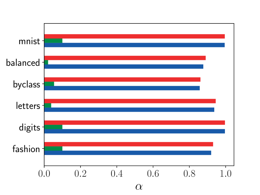
(a) Model accuracy ($n_{b}=64$) for the three learning algorithms. Red: shuffled; green: sorted by class; blue: block-random.

(b) Model accuracy of block-random algorithm as a function of $\nicefrac{{n_{b}}}{{n_{c}}}$. Red squares: “fashion”; green diamonds: “digits”; blue circles: “letters”; orange pentagon: “byclass”; purple hexagon: “balanced”; burgundy crosses: “mnist”.

Figure 2: Model accuracy, $\alpha=\nicefrac{{\text{number of correctly classified images}}}{{\text{total number of images}}}$, on validation data set for different benchmark cases.

3.2 Channel flow

To evaluate the performance of the algorithm in an exascale-like setting, we developed a DNN model for the “closure problem” for large eddy simulations (LES) in computational fluid dynamics. DNS of turbulent flows, in which all the physical length scales are resolved explicitly, require large computational resources and are often unfeasible for engineering and design applications. LES alleviate the computational requirements by resolving the large-scale motions and modeling the SGS, i.e., the length scales that are not resolved by the discretization grid. In computational fluid dynamics, LES solve the filtered Navier-Stokes equations, presented here in their incompressible form:

$$\frac{\partial\overline{u}_{i}}{\partial t}+\frac{\partial}{\partial x_{j}}\left(\overline{u}_{i}\overline{u}_{i}\right) =\frac{\partial}{\partial x_{j}}\left(\nu\frac{\partial\overline{u}_{i}}{\partial x_{j}}\right)-\frac{1}{\rho}\frac{\partial\overline{p}}{\partial x_{i}}-\frac{\partial\tau_{ij}}{\partial x_{j}}$$ (4)

$$\frac{\partial\overline{u}_{i}}{\partial x_{i}} =0$$ (5)

where $i$ and $j=1,2,3$; $x_{i}$ is the coordinate; $u_{i}$ is the velocity in the $x_{i}$ direction; $p$ is the pressure; $\nu$ is the kinematic viscosity; $\overline{\cdot}$ is the filtering operation, defined for an variable $\phi$ as $\overline{\phi}=\int_{\mathcal{D}}\phi(x)G(x,x^{\prime})\,\mathrm{d}{}x^{\prime}$, where $G(x,x^{\prime})$ is a filter function and $\mathcal{D}$ is the domain; and $\tau_{ij}$ is the SGS stress defined as $\tau_{ij}=\overline{u_{i}u_{j}}-\overline{u}_{i}\overline{u}_{j}$. The LES system of equations is unclosed because of the SGS stress term and requires a model for the SGS. Extensive work has been done to determine appropriate models for the SGS stress [18, 19, 20, 21]. For example, an early approach [22] uses an eddy viscosity closure that relates resolved velocity gradients to the SGS stress according to:

$$\tau_{ij}=-2(C_{s}\overline{\Delta})^{2}|\overline{S}|\overline{S}_{ij}$$ (6)

where $\overline{S}_{ij}=\nicefrac{{1}}{{2}}\left(\frac{\partial\overline{u}_{i}}{\partial x_{j}}+\frac{\partial\overline{u}_{j}}{\partial x_{i}}\right)$, $|\overline{S}|=\sqrt{2\overline{S}_{ij}\overline{S}_{ij}}$, $\overline{\Delta}$ is the filter length scale, and $C_{s}$ is a constant determined through the DNS of turbulent flows. Though SGS models have received much attention, because they are often tuned to simple configurations, the accuracy of these models continues to be problematic in a wide range of flows. In this section, we will use deep learning to construct a SGS stress model for $\tau_{12}$.

We emphasize that the objective of this work is not to derive the most accurate SGS model for turbulence, which has been a focus of recent investigations using deep learning [23, 24]; rather, it is to illustrate how to use DNS data from exascale-like simulations to develop an accurate model in the context of distributed, heterogeneous data. As such, we will use the DNS of an incompressible channel flow at a friction Reynolds number ($Re_{\tau}$) of 5186 by Lee and Moser [25]. The simulations were performed using the code PoongBack [26, 27], with 242 billion degrees of freedom (10240 in $x$, 1536 in $y$, and 7680 in $z$), and was run on 52488 cores, using approximately 400 million core hours of computation. The incompressible channel flow exhibits high inhomogeneity and anisotropy, as shown in Figure 3, from the presence of the walls. This makes it a challenging test case for the block-random algorithm because there will be a high bias between data from each spatial block.

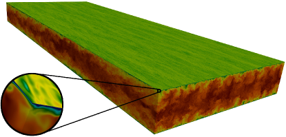
Figure 3: Streamwise velocity and wall-shear stress (inset) in the turbulent channel flow DNS. Figure generated by Dr. Myoungkyu Lee, using data from [25]

3.2.1 Data generation process

To get data for constructing a SGS model, first the nonlinear $u_{i}u_{j}$ terms are computed from the DNS velocity fields. A circular Fourier cutoff filter is then applied to the resulting fields, and $\tau_{ij}$ is computed from the filtered fields. The cutoff wavelength is chosen as $\lambda^{+}\approx 1500$ in the wall-parallel directions using insights from Lee and Moser [28]. This results in a grid of dimensions $(200,1536,128)$ in $(x,y,z)$ with more than 39 million data points. The input model variables are the three filtered velocities and nine filtered velocity gradients. The model is therefore learning a pointwise functional form:

$$\tau_{ij}|_{k}=f\left(\overline{u}_{i}|_{k},\left.\frac{\partial\overline{u}_{i}}{\partial x_{j}}\right|_{k}\right)$$ (7)

where $k$ denotes a point in the domain. ,The resulting data are then arranged into spatial blocks of size $(16,16,16)$ in $(x,y,z)$, with each block representing a computational node. In this setting, there will be a total of 9600 nodes containing data, which mimics a distributed large-scale computation.

3.2.2 Neural network architecture

The neural network architecture is a feed-forward, fully connected DNN. The hidden layers each comprise fully connected nodes. The first hidden layer contains a leaky rectified linear unit activation function:

$$y=R(x)=\begin{cases}x,&\text{ if }x\geq 0,\\ \gamma x,&\text{ otherwise, }\end{cases}$$ (8)

where $x$ is the layer input vector, $y$ is the layer output vector, and $\gamma=10^{-2}$ is a small slope. The other hidden layers contain a hyperbolic tangent activation function. The final network layer does not contain an activation function. The loss used to train the network is a mean squared error loss function. The specific SGD algorithm for this work is the Adam optimizer [15] because it presents many more advantages than traditional SGD by maintaining a per-parameter learning rate, which is adapted during training based on exponential moving averages of the first and second moments of the gradients. The deep learning framework was implemented through Keras [16] with the TensorFlow backend [17]. To find a reasonably accurate model for this study, a sweep of the model’s hyperparameters was performed, exploring the following combinations: the initial learning rate was varied from $10^{-2}$ to $10^{-5}$; the number of layers, $L$, was varied from 2 to 16; and the number of nodes in each layer was varied from 8 to 512. The sweeps were performed on the 1 million samples from the fully shuffled training data set. A neural network comprising an initial learning rate of $10^{-4}$, four hidden layers, and 128 nodes in each layer (for a total of 68000 trainable parameters) led to a model that was accurate without necessitating more than eight hours of training on an Intel Skylake workstation. This set of model hyperparameters is used in all subsequent results.

3.2.3 Assessments of learning algorithm performance

In this section, we present the results of the three different learning algorithms presented in this work: (i) fully shuffling all the data; (ii) using the data as they are in the high performance computing simulation (block-unshuffled), (iii) accessing the data in block-random fashion, as discussed in Section 2. Model quantities are denoted by superscript $\cdot^{m}$, and quantities computed with respect to the training and validation data sets are subscripted with $t$ and $v$, respectively. The mean squared error is defined as $\epsilon=\frac{1}{|\mathcal{D}|}\sum_{i\in\mathcal{D}}(\tau_{12}-\tau_{12}^{m})^{2}$, where $\mathcal{D}$ denotes the data set, and $|\cdot|$ is the cardinality of the set. The physics model used for comparisons is the Wall Adapting Local Eddy-Viscosity (WALE) model [29], a model specifically designed for LES of wall-bounded flows.

The training and validation mean squared error, $\epsilon_{t}$ and $\epsilon_{v}$, respectively, are shown in Figure 4 for the three different learning algorithms as a function of the batch size, $n_{b}$. The training error for the shuffled case reaches a minimum at $n_{b}=256$ and increases for higher $n_{b}$. The validation error, however, remains constant and smaller than the other two algorithms. The training error for the block-unshuffled algorithm is less than that for the block-random algorithm, though the validation error is three times larger than the other algorithms. This indicates that the model is capturing the batches of data toward the end of the training iteration but fails to adequately represent the full range of data. The training error decreases as a function of batch size because it is able to get a more representative data batch. This results, however, in an increasing validation error because it overfits the data available at the end of the training iteration. The block-random algorithms exhibits a validation error that is approximately $10\%$ higher than the shuffled algorithm, and it remains small as the batch size increases. For the remaining results presented in this section, the batch size is fixed at 256.

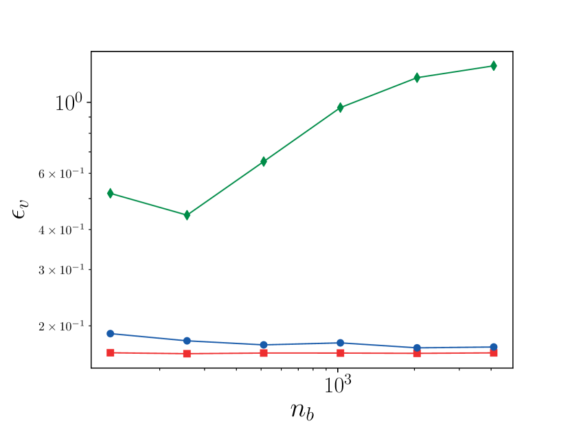
(a) Training error, $\epsilon_{t}$.

(b) Validation error, $\epsilon_{v}$.

Figure 4: Mean squared error for the three different learning algorithms as a function of the batch size. Red squares: shuffled; green diamonds: block-unshuffled; blue circles: block-random.

The normalized probability density function (PDF) of the error and the conditional means of the predictions are shown in Figure 5. The shuffled algorithm exhibits a sharp PDF of the error and a conditional means of the predictions identical to the filtered DNS throughout the channel domain. The block-random algorithm has a similar error PDF but underpredicts the peak $\tau_{12}$ by approximately $8\%$. The block-unshuffled algorithm fails to capture the conditional means throughout the channel. The WALE physics model overpredicts the peak $\tau_{12}$ by a factor of two and predicts that the peak occurs closer to the channel centerline. The WALE error PDF has a higher variance than the shuffled and block-random algorithms.

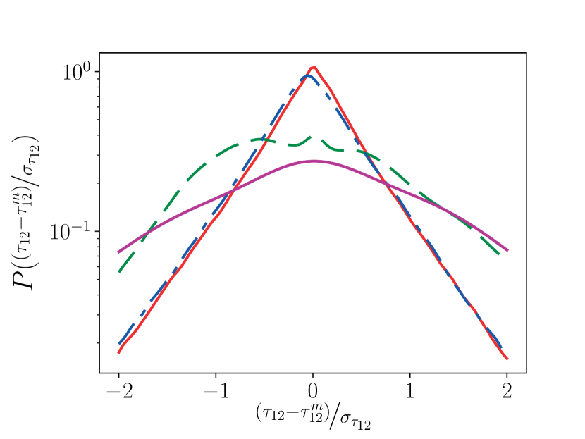
(a) Probability density function of the error normalized by the standard deviation of $\tau_{12}$.

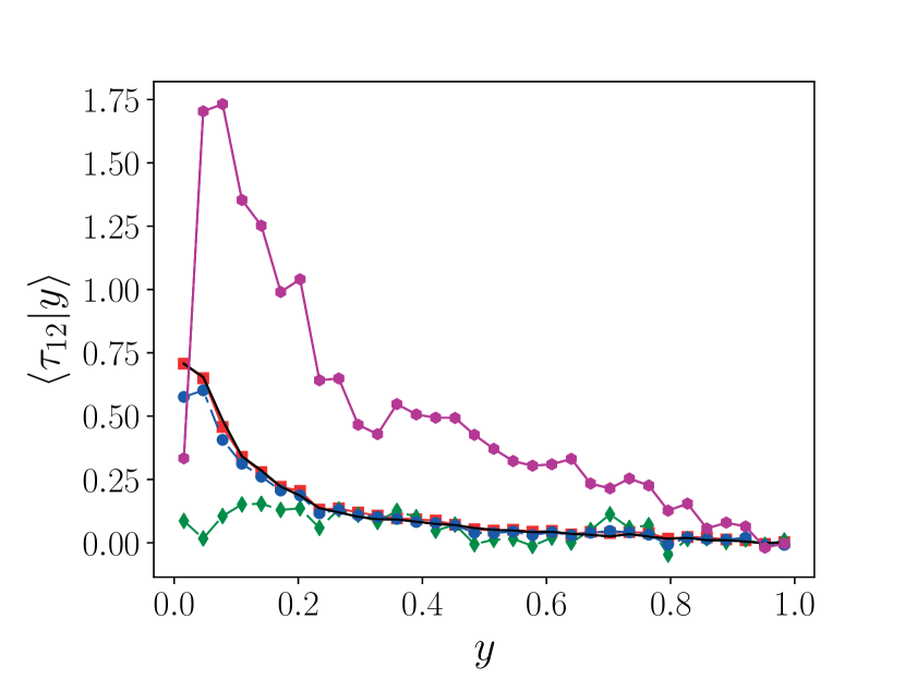
(b) Conditional means as a function of wall distance, $y^{+}=Re_{\tau}y$.

Figure 5: Model accuracy on validation data set. Red squares and solid: shuffled; green diamonds and dashed: block-unshuffled; blue circles and dash-dotted: block-random; purple hexagons and solid: WALE physics model; black solid: filtered DNS

As evidenced by these results, the key factor determining the performance of the model is the order of the blocks used by the SGD algorithm to adjust the model parameters. To quantify the difference between the learning algorithms, we use the Jensen-Shannon divergence [30, 31], a measure of the similarity between two PDFs. It is a symmetric version of the Kullback-Leibler divergence [32], and it is defined as:

$$J(Q,R)=\frac{1}{2}\left(D(Q,M)+D(R,M)\right)$$ (9)

where $D(Q,R)=\sum_{i=1}^{n}R(i)\ln{\left(\frac{R(i)}{Q(i)}\right)}$; $M=\nicefrac{{1}}{{2}}\left(Q+R\right)$; $Q$ and $R$ are PDFs of length $n$; and $0\leq J(Q,R)\leq\ln{(2)}$. Low values indicate more similarity between $Q$ and $R$. The Jensen-Shannon divergence has several advantages compared to the Kullback-Leibler divergence: symmetry, i.e., $J(Q,R)=J(R,Q)$, bounded, and variable support. This metric is used to quantify the difference between the different PDFs: the PDF of $\tau_{12}$ in the validation data set, $Y=P(\tau_{12}\in\mathcal{D}_{v})$, and the PDF of a given batch, $Y_{b}=P(\tau_{12}\in\mathcal{D}_{b})$, where $\mathcal{D}_{b}$ is the set of data in batch $b$. We compare (i) how the data in each batch are representative of the data in the entire domain by computing $J(Y,Y_{b})$ for all the batches in an epoch and (ii) how the data in each batch vary compared to the previous batch by computing $J(Y_{b-1},Y_{b})$.

Figure 6 illustrates the different metrics for the three different learning algorithms. For the fully shuffled case, each batch exhibits a PDF similar to that of the entire data set. The difference between $Y$ and $Y_{b}$ for the block-random case is higher but remains constant during the training epoch. For the block-unshuffled case, there is a clear structure to $J(Y,Y_{b})$ because of the heterogeneity of the data near the channel walls (beginning and ending of the training epoch). For all three algorithms, the difference between each subsequent batch is negligible. These results indicate that ensuring that $J(Y,Y_{b})$ remains less than 0.2 and constant throughout the training epoch is a criteria for achieving high model accuracy.

(a) Comparison between each batch and the entire data set.

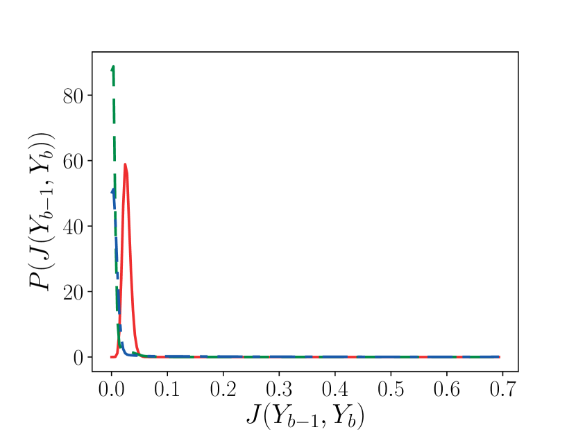
(b) Comparison between subsequent batches.

Figure 6: Characterizing the differences between batches. Solid red: shuffled; dashed green: block-unshuffled; dash-dotted blue: block-random.

4 Conclusions

Effectively training DNN models often assumes that the SGD algorithm processes data in batches of data that have been randomized prior to model training. This is expected to be prohibitively expensive for in situ model training from the perspective of communication between computing nodes, as illustrated in Figure 1. We showed that the SGD algorithm can still train an effective model if the batches are processed in random order even if the batches are each comprised of similar data. In this work, we demonstrated a block-random learning algorithm for training DNNs in the context of distributed heterogeneous data for data parallelism learning, a situation that will be increasingly common as the exascale era approaches and models are trained in situ. The block-random learning algorithm was tested on several different cases. For the benchmark EMNIST data sets, the block-random algorithm achieves accuracy similar to the traditional fully shuffled learning algorithm. The performance decreases slightly as the ratio of the batch size to the number of classes increases. To demonstrate the efficacy of the block-random algorithm for exascale-type simulations, we used a DNS simulation of turbulent channel flow to construct a LES SGS model. The model constructed using the block-random algorithm performed significantly better than the block-unshuffled learning model and is within $8\%$ of the fully shuffled model. Using the Jensen-Shannon divergence metric, we analyzed the characteristics of the batches used by the SGD to inform a criteria for successfully constructing a DNN model for distributed heterogeneous data.

This work — including neural network models, analysis scripts, Jupyter notebooks, and figures — can be publicly accessed at the project’s GitHub page. Traditional machine learning algorithms were implemented through scikit-learn [33] and the deep learning algorithms through Keras [16] with the TensorFlow backend [17].

References

References

- Lecun et al. [2015] Y. Lecun, Y. Bengio, G. Hinton, Deep learning, Nature 521 (2015) 436–444. doi:doi:10.1038/nature14539.
- Schmidhuber [2015] J. Schmidhuber, Deep Learning in neural networks: An overview, Neural Networks 61 (2015) 85–117. URL: http://dx.doi.org/10.1016/j.neunet.2014.09.003. doi:doi:10.1016/j.neunet.2014.09.003.
- Prieto et al. [2016] A. Prieto, B. Prieto, E. M. Ortigosa, E. Ros, F. Pelayo, J. Ortega, I. Rojas, Neural networks: An overview of early research, current frameworks and new challenges, Neurocomputing (2016). doi:doi:10.1016/j.neucom.2016.06.014.
- Goodfellow et al. [2016] I. Goodfellow, Y. Bengio, A. Courville, Deep Learning, MIT Press, 2016. URL: http://www.deeplearningbook.org.
- Liu et al. [2017] W. Liu, Z. Wang, X. Liu, N. Zeng, Y. Liu, F. E. Alsaadi, A survey of deep neural network architectures and their applications, Neurocomputing (2017). doi:doi:10.1016/j.neucom.2016.12.038.
- Ling et al. [2016] J. Ling, A. Kurzawski, J. Templeton, Reynolds averaged turbulence modelling using deep neural networks with embedded invariance, Journal of Fluid Mechanics 807 (2016) 155–166.
- Duraisamy et al. [2015] K. Duraisamy, Z. J. Zhang, A. P. Singh, New approaches in turbulence and transition modeling using data-driven techniques, in: 53rd AIAA Aerospace Sciences Meeting, 2015, p. 1284.
- Duraisamy et al. [2019] K. Duraisamy, G. Iaccarino, H. Xiao, Turbulence modeling in the age of data, Annual Review of Fluid Mechanics 51 (2019) 357–377.
- Zinkevich et al. [2010] M. Zinkevich, M. Weimer, L. Li, A. J. Smola, Parallelized stochastic gradient descent, in: Advances in neural information processing systems, 2010, pp. 2595–2603.
- Bottou [2010] L. Bottou, Large-scale machine learning with stochastic gradient descent, in: Proceedings of COMPSTAT’2010, Springer, 2010, pp. 177–186.
- Kingma and Ba [2014] D. P. Kingma, J. Ba, Adam: A method for stochastic optimization, arXiv preprint arXiv:1412.6980 (2014).
- Tieleman and Hinton [2012] T. Tieleman, G. Hinton, Lecture 6.5-rmsprop: Divide the gradient by a running average of its recent magnitude, COURSERA: Neural networks for machine learning 4 (2012) 26–31.
- Duchi et al. [2011] J. Duchi, E. Hazan, Y. Singer, Adaptive subgradient methods for online learning and stochastic optimization, Journal of Machine Learning Research 12 (2011) 2121–2159.
- Cohen et al. [2017] G. Cohen, S. Afshar, J. Tapson, A. van Schaik, EMNIST: an extension of MNIST to handwritten letters (2017). URL: http://arxiv.org/abs/1702.05373.
- Kingma and Ba [2014] D. P. Kingma, J. Ba, Adam: A Method for Stochastic Optimization (2014). URL: http://arxiv.org/abs/1412.6980.
- Chollet et al. [2015] F. Chollet, et al., Keras, https://keras.io, 2015.
- Abadi et al. [2015] M. Abadi, A. Agarwal, P. Barham, E. Brevdo, Z. Chen, C. Citro, G. S. Corrado, A. Davis, J. Dean, M. Devin, S. Ghemawat, I. Goodfellow, A. Harp, G. Irving, M. Isard, Y. Jia, R. Jozefowicz, L. Kaiser, M. Kudlur, J. Levenberg, D. Mané, R. Monga, S. Moore, D. Murray, C. Olah, M. Schuster, J. Shlens, B. Steiner, I. Sutskever, K. Talwar, P. Tucker, V. Vanhoucke, V. Vasudevan, F. Viégas, O. Vinyals, P. Warden, M. Wattenberg, M. Wicke, Y. Yu, X. Zheng, TensorFlow: Large-scale machine learning on heterogeneous systems, 2015. URL: http://tensorflow.org/, software available from tensorflow.org.
- Rogallo and Moin [1984] R. S. Rogallo, P. Moin, Numerical Simulation of Turbulent Flows, Annu. Rev. Fluid Mech. 16 (1984) 99–137. URL: http://www.annualreviews.org/doi/10.1146/annurev.fl.16.010184.000531. doi:doi:10.1146/annurev.fl.16.010184.000531.
- Lesieur [1996] M. Lesieur, New Trends in Large-Eddy Simulations of Turbulence, Annu. Rev. Fluid Mech. 28 (1996) 45–82. URL: http://fluid.annualreviews.org/cgi/doi/10.1146/annurev.fluid.28.1.45. doi:doi:10.1146/annurev.fluid.28.1.45.
- Piomelli [1999] U. Piomelli, Large-eddy simulation: achievements and challenges, Prog. Aerosp. Sci. 35 (1999) 335–362. URL: http://linkinghub.elsevier.com/retrieve/pii/S0376042198000141. doi:doi:10.1016/S0376-0421(98)00014-1.
- Meneveau and Katz [2000] C. Meneveau, J. Katz, Scale-Invariance and Turbulence Models for Large-Eddy Simulation, Annu. Rev. Fluid Mech. 32 (2000) 1–32. URL: http://www.annualreviews.org/doi/10.1146/annurev.fluid.32.1.1. doi:doi:10.1146/annurev.fluid.32.1.1.
- SMAGORINSKY [1963] J. SMAGORINSKY, GENERAL CIRCULATION EXPERIMENTS WITH THE PRIMITIVE EQUATIONS, Mon. Weather Rev. 91 (1963) 99–164. URL: http://journals.ametsoc.org/doi/abs/10.1175/1520-0493(1963)091{%}3C0099:GCEWTP{%}3E2.3.CO;2http://journals.ametsoc.org/doi/abs/10.1175/1520-0493{%}281963{%}29091{%}3C0099{%}3AGCEWTP{%}3E2.3.CO{%}3B2. doi:doi:10.1175/1520-0493(1963)091<0099:GCEWTP>2.3.CO;2.
- Ling et al. [2016] J. Ling, A. Kurzawski, J. Templeton, Reynolds averaged turbulence modelling using deep neural networks with embedded invariance, J. Fluid Mech. (2016). doi:doi:10.1017/jfm.2016.615.
- Maulik and San [2017] R. Maulik, O. San, A neural network approach for the blind deconvolution of turbulent flows, J. Fluid Mech. 831 (2017) 151–181. URL: https://www.cambridge.org/core/product/identifier/S0022112017006371/type/journal{_}article. doi:doi:10.1017/jfm.2017.637.
- Lee and Moser [2015] M. Lee, R. D. Moser, Direct numerical simulation of turbulent channel flow up to , Journal of Fluid Mechanics 774 (2015) 395–415.
- Lee et al. [2013] M. Lee, N. Malaya, R. D. Moser, Petascale direct numerical simulation of turbulent channel flow on up to 786k cores, in: Proceedings of the International Conference on High Performance Computing, Networking, Storage and Analysis, ACM, 2013, p. 61.
- Lee et al. [2014] M. Lee, R. Ulerich, N. Malaya, R. D. Moser, Experiences from leadership computing in simulations of turbulent fluid flows, Computing in Science & Engineering 16 (2014) 24–31.
- Lee and Moser [2019] M. Lee, R. D. Moser, Spectral analysis of the budget equation in turbulent channel flows at high reynolds number, Journal of Fluid Mechanics 860 (2019) 886–938. doi:doi:10.1017/jfm.2018.903.
- Ducros et al. [1998] F. Ducros, F. Nicoud, T. Poinsot, Wall-adapting local eddy-viscosity models for simulations in complex geometries, Numer. Methods Fluid Dyn. VI (1998) 293–299.
- Endres and Schindelin [2003] D. M. Endres, J. E. Schindelin, A new metric for probability distributions, 2003. doi:doi:10.1109/TIT.2003.813506.
- Österreicher and Vajda [2003] F. Österreicher, I. Vajda, A new class of metric divergences on probability spaces and its applicability in statistics, Ann. Inst. Stat. Math. (2003). doi:doi:10.1007/BF02517812.
- Kullback [1987] S. Kullback, Letters to the Editor, Am. Stat. 41 (1987) 338–341. URL: http://www.tandfonline.com/doi/abs/10.1080/00031305.1987.10475510. doi:doi:10.1080/00031305.1987.10475510.
- Pedregosa et al. [2011] F. Pedregosa, G. Varoquaux, A. Gramfort, V. Michel, B. Thirion, O. Grisel, M. Blondel, P. Prettenhofer, R. Weiss, V. Dubourg, J. Vanderplas, A. Passos, D. Cournapeau, M. Brucher, M. Perrot, E. Duchesnay, Scikit-learn: Machine Learning in Python, J. Mach. Learn. Res. (2011). doi:doi:10.1007/s13398-014-0173-7.2.