Sparse versions of the Cayley–Bacharach Theorem

Abstract.

We give combinatorial generalizations of the Cayley–Bacharach theorem and induced map.

1. Introduction

The Cayley–Bacharach theorem states that, given two cubic curves in the projective plane that meet in nine points, any other cubic that passes through eight of the points, contains also the ninth. As with many attributions in Mathematics, it is known that the Cayley–Bacharach theorem is originally due to Chasles; the article [EGH96] contains a thorough historical account of this result, including the roles of Cayley and Bacharach, as well as many geometric generalizations.

The Cayley–Bacharach theorem provides a map assigning a point in the plane to eight given points. More precisely, given eight points in the affine plane ${\mathbb{C}}^{2}$, the set of cubic polynomials in two variables that vanish at these points is a two dimensional vector space, at least if no three of the points are on a line, and no six lie on a conic. If $F(x,y)$, $G(x,y)$ form a basis of this vector space, Bézout’s Theorem implies that $F$ and $G$ have nine common zeros (in the projective plane) counting multiplicity. For most choices of eight points, all the multiplicities equal $1$, so a ninth point is determined. Again, for most choices of eight points, this ninth point lies in the affine plane. This is a natural map from a dense subset of $({\mathbb{C}}^{2})^{8}$ to ${\mathbb{C}}^{2}$. We call this the extra point map, $\Upsilon$.

The map $\Upsilon$ is rational, and explicit formulas for it can be found in the article [RRS15]. We give a different proof of rationality, as well as alternative formulas, in Section 2. While our formulas are less beautiful and more complicated than those in [RRS15], and no one in their right mind would use them in a practical context, they do have one very positive attribute: they can be naturally generalized.

The generalizations we are interested in are of the following form

A choice of $N$ generic points in ${\mathbb{C}}^{d}$ gives rise to $d$ hypersurfaces satisfying given constraints, and it turns out that those hypersurfaces meet in exactly $N+1$ points.

The constraints we consider are combinatorial in nature: we fix the monomials that appear in the defining equations of the corresponding hypersurfaces. These support sets must be carefully chosen; in Section 5, we call them Chasles configurations and Chasles structures. While Chasles’ work has received significant recognition (his name is on the Eiffel tower), we thought it appropriate to name our generalizations in his honor.

Our main result, Theorem 5.3, states that the extra point map arising in this more general situation is still rational. The proof is essentially the same as our proof that $\Upsilon$ is rational (see Theorem 2.1), and consequently also produces explicit formulas.

The key ingredient we use to compute $\Upsilon$ and its generalizations is the notion of resultant. The well-known resultant of two univariate polynomials $f$ and $g$ is a polynomial in the coefficients of $f$ and $g$ that vanishes precisely when $f$ and $g$ have a common factor. Resultants are a very important tool when solving polynomial equations, due to their fundamental role in elimination theory. This has spurred much interest in resultants, and especially in explicit formulas for resultants. We make use of the following fact (that is made precise in Theorem 4.11):

The product of the coordinates of the roots of a system of polynomial equations is a rational function of the coefficients of the system, that can be expressed in terms of resultants.

This result has been known since the late 1990s; see [K97, CDS98, R97] and also [PS93]. (In this article, we use the version from [DS15].) Its relevance is that it allows us to express the coordinates of the point we are interested in, in terms of the coordinates of the points we are given and the coefficients of the polynomials that define the hypersurfaces containing those points. Those coefficients can also be expressed as rational functions of the coordinates of the given points, since we have fixed the monomials that appear in those polynomials.

Outline

In Section 2, we prove that $\Upsilon$ is rational by giving an explicit formula in terms of Sylvester resultants. Section 3 explains our motivation for considering $\Upsilon$ in the first place. Section 4 is a technical section containing results needed to generalize the Cayley–Bacharach theorem. The paper becomes readable again in Section 5, where we introduce our generalizations, and Section 6 contains infinitely many examples.

Acknowledgments

This project has benefited from visits by the authors to each other’s institutions. We also discussed this material during the joint meeting of the AMS and the RSME in Seville in the Summer of 2003. We are very grateful to Bernd Sturmfels, for his thoughtful advice, and for directing us to the Cayley octads example in Subsection 6.4. Thanks also to Frank Sottile for productive conversations.

2. The extra point map is rational

We start by showing that the map arising from the Cayley–Bacharach theorem is rational.

Theorem 2.1.

Let $\Upsilon$ be the map that assigns, to eight generic points in the plane, a ninth point determined by the Cayley–Bacharach theorem. The map $\Upsilon$ is rational.

Proof.

We show that $\Upsilon$ is rational by giving an explicit formula. We denote the eight given points by $\rho_{i}=(a_{i},b_{i})\in({\mathbb{C}}^{*})^{2},1\leq i\leq 8$. By the genericity assumption, we may assume that two linearly independent cubic polynomials vanishing on $\rho_{1},\dots,\rho_{8}$ are of the form

$$F(x,y)=x^{3}+\kappa_{21}x^{2}y+\kappa_{12}xy^{2}+\kappa_{20}x^{2}+\kappa_{02}y^{2}+\kappa_{11}xy+\kappa_{10}x+\kappa_{01}y+\kappa_{00}$$

$$G(x,y)=y^{3}+\lambda_{21}x^{2}y+\lambda_{12}xy^{2}+\lambda_{20}x^{2}+\lambda_{02}y^{2}+\lambda_{11}xy+\lambda_{10}x+\lambda_{01}y+\lambda_{00}$$

Let $M$ be the matrix whose rows are $[a_{i}^{2}b_{i},a_{i}b_{i}^{2},a_{i}^{2},b_{i}^{2},a_{i}b_{i},a_{i},b_{i},1]$ for $i=1,\dots,8$. Then $[\kappa_{21},\kappa_{12},\kappa_{20},\kappa_{02},\kappa_{11},\kappa_{10}\kappa_{01},\kappa_{00}]^{t}$ is a solution of

$$Mv=[-a_{1}^{3},\dots,-a_{8}^{3}]^{t},$$

and $[\lambda_{21},\lambda_{12},\lambda_{20},\lambda_{02},\lambda_{11},\lambda_{10}\lambda_{01},\lambda_{00}]^{t}$ is a solution of

$$Mv=[-b_{1}^{3},\dots,-b_{8}^{3}]^{t}.$$

Again, as $\rho_{1},\dots,\rho_{8}$ are generic, we may assume that $\det(M)\neq 0$, and consequently we may explicitly write the coefficients $\kappa_{ij}$ and $\lambda_{ij}$ as ratios of polynomials in $a_{i},b_{j}$ using Cramer’s rule. For instance

$$\kappa_{00}=\frac{\det\begin{bmatrix}a_{1}^{2}b_{1}&a_{1}b_{1}^{2}&a_{1}^{2}&b_{1}^{2}&a_{1}b_{1}&a_{1}&b_{1}&-a_{1}^{3}\\ a_{2}^{2}b_{2}&a_{2}b_{2}^{2}&a_{2}^{2}&b_{2}^{2}&a_{2}b_{2}&a_{2}&b_{2}&-a_{2}^{3}\\ a_{3}^{2}b_{3}&a_{3}b_{3}^{2}&a_{3}^{2}&b_{3}^{2}&a_{3}b_{3}&a_{3}&b_{3}&-a_{3}^{3}\\ a_{4}^{2}b_{4}&a_{4}b_{4}^{2}&a_{4}^{2}&b_{4}^{2}&a_{4}b_{4}&a_{4}&b_{4}&-a_{4}^{3}\\ a_{5}^{2}b_{5}&a_{5}b_{5}^{2}&a_{5}^{2}&b_{5}^{2}&a_{5}b_{5}&a_{5}&b_{5}&-a_{5}^{3}\\ a_{6}^{2}b_{6}&a_{6}b_{6}^{2}&a_{6}^{2}&b_{6}^{2}&a_{6}b_{6}&a_{6}&b_{6}&-a_{6}^{3}\\ a_{7}^{2}b_{7}&a_{7}b_{7}^{2}&a_{7}^{2}&b_{7}^{2}&a_{7}b_{7}&a_{7}&b_{7}&-a_{7}^{3}\\ a_{8}^{2}b_{8}&a_{8}b_{8}^{2}&a_{8}^{2}&b_{8}^{2}&a_{8}b_{8}&a_{8}&b_{8}&-a_{8}^{3}\\ \end{bmatrix}}{\det M}$$

Now consider $F$ and $G$ as polynomials in the variable $x$, with coefficients that are polynomials in $y$, and take the resultant to eliminate the variable $x$. The roots of this resultant (as a polynomial in $y$) are the $y$-coordinates of the nine solutions of $F=G=0$. Consequently, the coefficient of $y^{0}$ in this resultant is the product of those nine $y$-coordinates. By taking resultant with respect to $y$, we can also obtain the product of the nine $x$-coordinates of the solutions of $F=G=0$.

The above calculation can be performed explicitly using a computer algebra system. We used Macaulay2 [M2] to compute the coefficients we are interested in, which are given below.

The zeroth coefficient for the resultant of $F$ and $G$ with respect to $y$ is:

$$R_{x}= \kappa_{02}^{3}\lambda_{00}^{2}-\kappa_{02}^{2}\kappa_{01}\lambda_{01}\lambda_{00}+\kappa_{02}\kappa_{01}^{2}\lambda_{02}\lambda_{00}+\kappa_{02}^{2}\kappa_{00}\lambda_{01}^{2}-2\kappa_{02}^{2}\kappa_{00}\lambda_{02}\lambda_{00}-\kappa_{02}\kappa_{01}\kappa_{00}\lambda_{02}\lambda_{01}+$$

$$\kappa_{02}\kappa_{00}^{2}\lambda_{02}^{2}-\kappa_{01}^{3}\lambda_{00}+3\kappa_{02}\kappa_{01}\kappa_{00}\lambda_{00}+\kappa_{01}^{2}\kappa_{00}\lambda_{01}-2\kappa_{02}\kappa_{00}^{2}\lambda_{01}-\kappa_{01}\kappa_{00}^{2}\lambda_{02}+\kappa_{00}^{3}$$

The zeroth coefficient for the resultant of $F$ and $G$ with respect to $x$ (exchange $\lambda$’s and $\kappa$’s) is:

$$R_{y}= \kappa_{00}^{2}\lambda_{20}^{3}-\kappa_{10}\kappa_{00}\lambda_{20}^{2}\lambda_{10}+\kappa_{20}\kappa_{00}\lambda_{20}\lambda_{10}^{2}+\kappa_{10}^{2}\lambda_{20}^{2}\lambda_{00}-2\kappa_{20}\kappa_{00}\lambda_{20}^{2}\lambda_{00}-\kappa_{20}\kappa_{10}\lambda_{20}\lambda_{10}\lambda_{00}+$$

$$\kappa_{20}^{2}\lambda_{20}\lambda_{00}^{2}-\kappa_{00}\lambda_{10}^{3}+3\kappa_{00}\lambda_{20}\lambda_{10}\lambda_{00}+\kappa_{10}\lambda_{10}^{2}\lambda_{00}-2\kappa_{10}\lambda_{20}\lambda_{00}^{2}-\kappa_{20}\lambda_{10}\lambda_{00}^{2}+\lambda_{00}^{3}$$

Then our ninth point, $\rho=(a,b)=\Upsilon(\rho_{1},\dots,\rho_{8})$, can be expressed as

$$a=\frac{R_{x}}{a_{1}\cdots a_{8}},\qquad b=\frac{R_{y}}{b_{1}\cdots b_{8}}.$$

∎

While the above formulas involve much division and high degree polynomials, their most significant feature, as has been mentioned before, is that they can be generalized. But this must wait until Section 5.

3. Hilbert

This version of the Cayley-Bacharach Theorem was central to Hilbert’s 1888 proof that there exist positive semidefinite (psd) ternary sextics which cannot be written as a sum of squares (sos) of real ternary cubics (see [H1888]). Hilbert starts with two real cubic polynomials $F(x,y)$ and $G(x,y)$ which have nine common zeros – $\{\rho_{j}\mid 1\leq j\leq 9\}$, no three on a line, no six on a conic. He shows how to construct a sextic $H$ which is singular at $\{\rho_{j}\mid 1\leq j\leq 8\}$ but so that $H(\rho_{9})>0$. By looking separately at the neighborhoods of the $\rho_{j}$’s and their complement, Hilbert shows that there exists $\lambda>0$ so that $f=F^{2}+G^{2}+\lambda H$ is psd; observe that $f(\rho_{j})=0$ for $1\leq j\leq 8$ and $f(\rho_{9})>0$. Suppose now that $f=\sum g_{k}^{2}$ for cubics $g_{k}$. Then $g_{k}(\rho_{j})=0$ for $1\leq j\leq 8$, and Cayley-Bacharach implies that $g_{k}(\rho_{9})=0$ for all $g_{k}$, a contradiction, which means that $f$ is not sos. The condition on $F,G$ ensures that they (and $H$) cannot be particularly simple, and no explicit example was constructed in the subsequent eighty years.

In 1969, R. M. Robinson (see [R69]), showed that Hilbert’s construction works with a simple pair $\{F,G\}$ which do not satisfy his restriction. He took $F(x,y)=x^{3}-x$ and $F(x,y)=y^{3}-y$, so that the $\rho_{j}$’s form the $3\times 3$ grid: $\{-1,0,1\}^{2}$. He then shows (in our notation) that $H(x,y)=(1-x^{2})(1-y^{2})(1-x^{2}-y^{2})$ fulfills the conditions of Hilbert’s construction and that one may even take $\lambda=1$. The resulting polynomial homogenizes to an even symmetric ternary sextic form:

$$R(x,y,z): =(x^{3}-xz^{2})^{2}+(y^{3}-yz^{2})^{2}+(x^{2}-z^{2})(y^{2}-z^{2})(z^{2}-x^{2}-y^{2})$$

$$=x^{6}+y^{6}+z^{6}-(x^{4}y^{2}+x^{2}y^{4}+x^{4}z^{2}+x^{2}z^{4}+y^{4}z^{2}+y^{2}z^{4})+3x^{2}y^{2}z^{2}.$$

Robinson proves that this form is psd, by writing $(x^{2}+y^{2})R(x,y,z)$ as a sum of squares. Hilbert’s argument shows that $R$ itself is not sos. The original eight zeros homogenize to $\{(\pm 1,\pm 1,1),(\pm 1,0,1),(0,\pm 1,1)\}$ and $R$ itself has two additional zeros “at infinity” $(1,\pm 1,0)$. The article [R00] contains further historical discussion on psd and sos forms.

Choi, Lam and the second author [CLR87] used Robinson’s example as a starting point to analyze all psd even symmetric sextics in $n\geq 3$. The second author [R07] generalized Robinson’s example and showed that Hilbert’s construction applies, as long as no four of the common zeros $\{\rho_{j}\}$ are on a line, and no seven are on a conic. That paper also contains many worked-out examples.

4. Sparse polynomial systems and sparse resultants

In this section, we collect results on sparse systems of polynomial equations that are necessary for our generalizations of the Cayley–Bacharach theorem.

A configuration of lattice points, or a configuration is a finite subset $A$ of ${\mathbb{Z}}^{d}$. The dimension of $A$, denoted by $\dim(A)$, is the dimension of the smallest affine subspace of ${\mathbb{R}}^{d}$ containing all points in $A$.

If $A$ is a configuration, ${\rm conv}(A)$ denotes the convex hull of the elements of $A$ in ${\mathbb{R}}^{d}$; ${\rm conv}(A)$ is a convex lattice polytope (a convex polytope whose vertices have integer coordinates).

A configuration $A$ is called saturated if $A={\rm conv}(A)\cap{\mathbb{Z}}^{d}$, that is, if $A$ equals the set of all lattice points in its convex hull.

If $A\subset{\mathbb{Z}}^{d}$ is a $d$-dimensional configuration, its normalized volume, denoted ${\rm vol}(A)$, is the Euclidean volume of ${\rm conv}(A)$, renormalized so that the unit simplex in ${\mathbb{Z}}^{d}$ has volume one. More explicitly, the ${\rm vol}(A)$ is $d!$ times the Euclidean volume of ${\rm conv}(A)$.

A Laurent polynomial is supported on a configuration $A$ if it is of the form $\sum_{u\in A}\lambda_{u}x^{u}\in{\mathbb{C}}[x_{1}^{\pm},\dots,x_{d}^{\pm}]$.

The following result, due to Kouchnirenko [K76], illustrates the connection between the combinatorics of configurations and systems of polynomial equations.

Theorem 4.1.

Let $A\subset{\mathbb{Z}}^{d}$ be a $d$-dimensional configuration, and let $F_{1},\dots,F_{d}$ be generic Laurent polynomials supported on $A$. Then the number of common roots of $F_{1},\dots,F_{d}$ (in $({\mathbb{C}}\smallsetminus\{0\})^{d}:=({\mathbb{C}}^{*})^{d}$) is ${\rm vol}(A)$.

Our next goal is to give the number of solutions to a system of Laurent polynomial equations, when the supports of the equations are not necessarily the same. A note on terminology: when we refer to sparse systems of equations, we mean a system of Laurent polynomial equations whose supports have been fixed. We start by introducing a generalization of the notion of volume.

Definition 4.2.

If $P\subset{\mathbb{R}}^{d}$ is a convex polytope and $\lambda\in{\mathbb{R}}$, let $\lambda P=\{\lambda u\mid u\in P\}$. If $P,Q\subset{\mathbb{R}}^{d}$ are polytopes, their Minkowski sum is $P+Q=\{u+v\mid u\in P,v\in Q\}$. Let $A_{1},\dots,A_{d}$ be configurations, and denote $P_{i}={\rm conv}(A_{i})$. The the mixed volume of $P_{1},\dots,P_{d}$ is

$${\rm mvol}(P_{1},\dots,P_{d}):=\frac{1}{d!}\sum_{k=1}^{d}(-1)^{d-k}\sum_{1\leq i_{1}<\cdots<i_{k}\leq d}{\rm vol}(P_{i_{1}}+\cdots+P_{i_{k}}).$$

The following result is known as the Bernstein, Kouchnirenko and Khovanskii (or BKK) theorem. In this form, it first appeared in  [B75].

Theorem 4.3.

Let $A_{1},\dots,A_{d}\subset{\mathbb{Z}}^{d}$ be configurations, and denote $P_{i}={\rm conv}(A_{i})$. For $1\leq i\leq d$, let $F_{i}=\sum_{a\in A_{i}}\lambda_{i,a}x^{a}$ be a Laurent polynomial with support contained in $A_{i}$. If the coefficients $\{\lambda_{i,a}\mid a\in A_{i},1\leq i\leq d\}$ are sufficiently generic, the system of polynomial equations $F_{1}(x)=\cdots=F_{d}(x)=0$ has precisely ${\rm mvol}(P_{1},\dots,P_{d})$ solutions in $({\mathbb{C}}^{*})^{d}$.

We now turn to sparse resultants. While a system of $d$ generic Laurent polynomial equations in $d$ variables has solutions (see Theorem 4.3), a system of $d+1$ Laurent polynomials in $d$ variables in general does not. The coefficients of the polynomials in such a system for which solutions exist are determined by a polynomial called the resultant.

As was mentioned in the introduction, resultants can be used to give an expression for the product (of the coordinates) of the roots of a sparse system. The earliest versions of this can be found in [K97, CDS98, R97, PS93]. In this article we use the formulas that appear in [DS15].

Our first task is to introduce resultants in general.

Definition 4.4.

Let $A_{0},A_{1},\dots,A_{d}$ be finite subsets of ${\mathbb{Z}}^{d}$, and let ${\mathscr{A}}=(A_{0},\dots,A_{d})$. Write $F_{i}=F_{i}(\lambda_{i},x)=\sum_{u\in A_{i}}\lambda_{i,u}x^{u}$ for a Laurent polynomial supported on $A_{i}$, where $\lambda_{i}=(\lambda_{i,u}\mid u\in A_{i})$ are variables representing the coefficients of $F_{i}$. Set $\lambda=(\lambda_{0},\dots,\lambda_{d})$. Let

$$\Omega_{{\mathscr{A}}}=\{(x,\lambda)\mid F_{0}(\lambda_{0},x)=\cdots=F_{d}(\lambda_{d},x)=0\}\subset({\mathbb{C}}^{*})^{d}\times\prod_{i=0}^{d}{\mathbb{P}}^{|A_{i}|-1}.$$

If the closure of the image of $\Omega_{{\mathscr{A}}}$ under the projection $({\mathbb{C}}^{*})^{d}\times\prod_{i=0}^{d}{\mathbb{P}}^{|A_{i}|-1}\to\prod_{i=0}^{d}{\mathbb{P}}^{|A_{i}|-1}$ has codimension $1$, then the resultant $\operatorname{Res}_{\mathscr{A}}(F_{0},\dots,F_{d})$ is defined to be the unique (up to sign) irreducible polynomial in ${\mathbb{Z}}[\lambda]$ which vanishes on this hypersurface. If this closure has codimension at least $2$, then we define $\operatorname{Res}_{\mathscr{A}}(F_{0},\dots,F_{d})=1$.

Example 4.5.

In our definitions, we have used the lattice ${\mathbb{Z}}^{d}$ as the ambient lattice without remarking upon it. In general, we may be given configurations that naturally live in lattices other than ${\mathbb{Z}}^{d}$, in which case, we need to change the way we compute resultants accordingly.

For instance, consider $A=\{(0,0,0),(0,1,0),(-1,0,2)\}\subset{\mathbb{Z}}^{3}$. Then $A$ generates a lattice $L$ which is isomorphic to ${\mathbb{Z}}^{2}$. If $F_{i}=\lambda_{i,1}+\lambda_{i,2}y+\lambda_{i,3}x^{-1}z^{2}$ are generic Laurent polynomials supported on $A$ for $i=1,2,3$, the system $F_{0}(x,y,z)=F_{1}(x,y,z)=F_{2}(x,y,z)=0$ has solutions in $({\mathbb{C}}^{*})^{3}$. On the other hand, we can also consider this as a system of $3$ equations in the two variables $(s,t)$ induced by the lattice $L$. This new system is $\lambda_{i,1}+\lambda_{i,2}s+\lambda_{i,3}t=0$ for $i=1,2,3$, whose solvability depends on the vanishing of the determinant of the $3\times 3$ matrix $[\lambda_{i,j}]$. Using the convention that the ambient lattice is $L$, this determinant is the resultant of our system.

In order to use the formulas in [DS15], what is needed is a power $\operatorname{Res}_{\mathscr{A}}(F_{0},\dots,F_{d})^{\mu_{{\mathscr{A}}}}$. The exponent $\mu_{{\mathscr{A}}}$ can be given a geometric or combinatorial definition; we use the combinatorial definition of $\mu_{\mathscr{A}}$ that can be found in [E10, Section 2.1].

We need a preliminary result. If $J\subset\{0,\dots,d\}$, set $A_{J}=\cup_{j\in J}A_{j}$. The following is [S94, Corollary 1.1].

Proposition 4.6.

With the notation of Definition 4.4, $\operatorname{Res}_{\mathscr{A}}(F_{0},\dots,F_{d})\neq 1$ if and only if there exists a unique subset $J_{0}\subset\{0,\dots,d\}$ such that

1. $\dim({\rm conv}(A_{J_{0}}))-|J_{0}|=-1$, and

2. for $J\subsetneq J_{0}$, $\dim({\rm conv}(A_{J}))-|J|>-1$.

Definition 4.7.

Let ${\mathscr{A}}$ as in Definition 4.4. Assuming that $\operatorname{Res}_{\mathscr{A}}(F_{0},\dots,F_{d})\neq 1$, let $J_{0}\subseteq\{0,\dots,d\}$ be as in Proposition 4.6, and consider $A_{J_{0}}\times\{1\}\subset{\mathbb{Z}}^{d+1}$. Let

$$\pi:{\mathbb{R}}^{d+1}\to{\mathbb{R}}^{d+1}/\operatorname{span}_{\mathbb{R}}(A_{J_{0}}\times\{1\})$$

be the projection, and let $\eta$ be a volume form on ${\mathbb{R}}^{d+1}/\operatorname{span}_{\mathbb{R}}(A_{J_{0}}\times\{1\})$ such that the volume of ${\mathbb{R}}^{d+1}/\big{(}\operatorname{span}_{\mathbb{R}}(A_{J_{0}}\times\{1\})+{\mathbb{Z}}^{d+1}\big{)}$ with respect to $\eta$ equals $(d+1-|J_{0}|)!$. We set

$$\mu_{\mathscr{A}}:=\left|\frac{\operatorname{span}_{\mathbb{R}}(A_{J_{0}}\times\{1\})\cap{\mathbb{Z}}^{d+1}}{\operatorname{span}_{\mathbb{Z}}(A_{J_{0}}\times\{1\})}\right|\cdot{\rm mvol}_{\eta}\bigg{(}\{{\rm conv}(\pi(A_{i}\times\{1\}))\mid i\in\{0,\dots,d\}\smallsetminus J_{0}\}\bigg{)}$$ (4.1)

where ${\rm mvol}_{\eta}$ denotes the mixed volume with respect to the volume form $\eta$.

There is one case where $\mu_{\mathscr{A}}$ is easy to compute.

Lemma 4.8.

Use the notation of Definitions 4.4 and 4.7. If each of the sets $A_{0},\dots,A_{d}$ spans ${\mathbb{Z}}^{d}$ as a lattice, then $\mu_{\mathscr{A}}=1$.

Proof.

In this case, $J_{0}=\{0,\dots,d\}$. We have also $\operatorname{span}_{\mathbb{R}}(A_{J_{0}}\times\{1\})\cap{\mathbb{Z}}^{d+1}=\operatorname{span}_{\mathbb{Z}}(A_{J_{0}}\times\{1\})$, so that the first factor in (4.1) equals $1$, and the second factor does not appear, since $\{0,\dots,d\}\smallsetminus J_{0}=\varnothing$. ∎

Definition 4.9.

Using the notation from Definitions 4.4 and 4.7, we set

$$\operatorname{mRes}_{\mathscr{A}}(F_{0},\dots,F_{d}):=\operatorname{Res}_{\mathscr{A}}(F_{0},\dots,F_{d})^{\mu_{\mathscr{A}}}.$$ (4.2)

Remark 4.10.

In [E10, DS15], the word resultant, and its corresponding notation, is used for the polynomial $\operatorname{mRes}_{\mathscr{A}}(\lambda)$. In this article, we follow the usual convention that resultants are irreducible polynomials.

Our goal is to state a formula from [DS15] that gives the product of the coordinates of the solutions of a sparse system of equations in terms of resultants. To do this, we need to introduce directional resultants.

Let $A_{1},\dots,A_{d}$ be finite subsets of ${\mathbb{Z}}^{d}$, and let $F_{1},\dots,F_{d}$ be Laurent polynomials such that the support of $F_{i}=\sum_{u\in A_{i}}\lambda_{i,u}x^{u}$ is (contained in) $A_{i}$. Let $v\in\operatorname{Hom}({\mathbb{Z}}^{d},{\mathbb{Z}})\cong{\mathbb{Z}}^{d}$. The weight of $u\in{\mathbb{Z}}^{d}$ with respect to $v$, denoted $v\cdot u$, is the image of $u$ under $v$. For $1\leq i\leq d$, let $A_{i,v}$ be the set of elements of $A_{i}$ with minimal weight with respect to $v$, and let $F_{i,v}=\sum_{u\in A_{i,v}}\lambda_{i,u}x^{u}$ be the restriction of $F_{i}$ to $A_{i,v}$. Note that $A_{i,v}$ is contained in a translate of the lattice $v^{\perp}=\{u\in{\mathbb{Z}}^{d}\mid v\cdot u=0\}\cong{\mathbb{Z}}^{d-1}$. Choose $\beta_{1,v},\dots,\beta_{d,v}\in{\mathbb{Z}}^{d}$ such that $A_{i,v}-\beta_{i,v}:=\{u-\beta_{i,v}\mid u\in A_{i,v}\}\subset v^{\perp}$, and let $G_{i,v}=\sum_{u\in A_{i}}\lambda_{i,u}x^{u-\beta_{i,v}}$. We denote

$$\operatorname{mRes}_{{\mathscr{A}},v}(F_{1,v},\dots,F_{d,v}):=\operatorname{mRes}_{\{A_{1,v},\dots,A_{d,v}\}}(G_{1,v},\dots,G_{d,v})$$ (4.3)

In the expression above, the resultant on the right hand side is constructed with respect to the ambient lattice $v^{\perp}$ as in Example 4.5. We have constructed a polynomial in the coefficients of the $F_{i,v}$, which is called a directional resultant. We note that it is independent of the choice of $\beta_{1,v},\dots,\beta_{d,v}$.

We are now ready to state the main result of this section, which is a special case of [DS15, Corollary 1.3].

Theorem 4.11.

Let $A_{1},\dots,A_{d}\subset{\mathbb{Z}}^{d}$ be configurations, and let $F_{1},\dots,F_{d}$ be Laurent polynomials supported on $A_{1},\dots,A_{d}$. Denote by $\mathscr{Z}(F_{1},\dots,F_{d})$ the set of solutions of $F_{1}(x)=\cdots=F_{d}(x)=0$ in $({\mathbb{C}}^{*})^{d}$. If $\rho\in\mathscr{Z}(F_{1},\dots,F_{d})$, let $m_{\rho}$ be its multiplicity as a solution of $F_{1}(x)=\cdots=F_{d}(x)=0$. Assume that for all $v\neq 0$, $v\in\operatorname{Hom}({\mathbb{Z}}^{d},{\mathbb{Z}})$, we have $\operatorname{mRes}_{{\mathscr{A}},v}(F_{1,v},\dots,F_{d,v})\neq 0$. For $1\leq i\leq d$, we have that

$$\prod_{\rho\in\mathscr{Z}(F_{1},\dots,F_{d})}\rho_{i}^{m_{\rho}}=\pm\prod\operatorname{mRes}_{{\mathscr{A}},v}(F_{1,v},\dots,F_{d,v})^{v\cdot e_{i}},$$ (4.4)

where the product on the right is over the primitive vectors in $\operatorname{Hom}({\mathbb{Z}}^{d},{\mathbb{Z}})$, and $e_{1},\dots,e_{d}$ are the standard unit vectors in ${\mathbb{Z}}^{d}$.

We note that by Proposition 4.6, if $v$ is not an inner normal of a codimension $1$ face of ${\rm conv}(A_{1})+\cdots+{\rm conv}(A_{d})$, then $\operatorname{mRes}_{{\mathscr{A}},v}(F_{1,v},\dots,F_{d,v})=1$. This implies that the product on the right hand side of (4.4) has finitely many factors different from $1$.

The $\pm$ sign in (4.4) is necessary, since resultants are only defined up to sign.

Remark 4.12.

The assumption in Theorem 4.11, that the directional resultants do not vanish, is a genericity assumption. It states that we are working with a system of Laurent polynomial equations such that none of the facial subsystems have a common root.

5. Chasles Configurations and Structures

In this section, we give combinatorial generalizations for the Cayley–Bacharach theorem.

Definition 5.1.

Let $A\subset{\mathbb{Z}}^{d}$ be a $d$-dimensional configuration, and write $|A|$ for the cardinality of $A$. Then $A$ is a Chasles configuration if $|A|+1={\rm vol}(A)+d$. A Chasles configuration $A\subset{\mathbb{Z}}^{d}$ is saturated if $A={\rm conv}(A)\cap{\mathbb{Z}}^{d}$.

If $A$ is a Chasles configuration, let $N={\rm vol}(A)-1$, so that $|A|=N+d$. Fix $N$ generic points in ${\mathbb{C}}^{d}$. The Laurent polynomials supported on $A$ that vanish on these $N$ points form a $d$-dimensional vector space. If $F_{1},\dots,F_{d}$ is a basis for this vector space, then by Theorem 4.1, the number of common zeros of $F_{1},\dots,F_{d}$ is $N+1$. This determines a map $\Upsilon_{A}$ from an open subset of $({\mathbb{C}}^{d})^{N}$ to ${\mathbb{C}}^{d}$.

Definition 5.2.

More generally, a Chasles structure consists of: two positive integers $N$ and $d$, a partition $d=k_{1}+\cdots+k_{\ell}$, and configurations $A_{1},\dots,A_{\ell}\subseteq{\mathbb{Z}}^{d}$ such that $|A_{i}|=N+k_{i}$, and ${\rm mvol}(\underbrace{A_{1},\dots,A_{1}}_{k_{1}\text{ times}},\underbrace{A_{2},\dots,A_{2}}_{k_{2}\text{ times}},\dots,\underbrace{A_{\ell},\dots,A_{\ell}}_{k_{\ell}\text{ times}})=N+1$. We denote ${\mathscr{A}}=\{A_{1},\dots,A_{\ell}\}$. We sometimes abuse notation and call ${\mathscr{A}}$ a Chasles structure.

Note that Chasles configuration is a Chasles structure for $N=|A|-\dim(A)$, $d=\dim(A)$, with partition $d=k_{1}$.

We now come to the main result in this article.

Theorem 5.3.

A Chasles structure ${\mathscr{A}}$ induces a rational map $\Upsilon_{{\mathscr{A}}}:[({\mathbb{C}}^{*})^{d}]^{N}\dashrightarrow({\mathbb{C}}^{*})^{d}$

Proof.

A Chasles structure is set up so that, if we fix $N$ general points $\rho_{1},\dots,\rho_{N}\in({\mathbb{C}}^{*})^{d}$, then for each $i=1,\dots,\ell$, those points determine a $k_{i}$-dimensional vector space of Laurent polynomials supported on $A_{i}$ that vanish on them. Picking a basis of each vector space, we obtain $k_{1}+\cdots+k_{\ell}=d$ polynomials $F_{1},\dots,F_{d}$, whose coefficients can be expressed as rational functions on the coordinates of $\rho_{1},\dots,\rho_{N}$.

Since the mixed volume of the corresponding Newton polytopes equals $N+1$, the Laurent polynomials $F_{1},\dots,F_{d}$ have $N+1$ common zeros in $({\mathbb{C}}^{*})^{d}$ by Theorem 4.3. Let $\rho_{N+1}$ be the point determined in this way. Note that the genericity assumption on $\rho_{1},\dots,\rho_{N}$ implies that $\rho_{N+1}\notin\{\rho_{1},\dots,\rho_{N}\}$.

On the other hand, for fixed $1\leq i\leq d$, the product of the $i$th coordinates of $\rho_{1},\dots,\rho_{N+1}$ can be expressed as a rational function on the coefficients of $F_{1},\dots,F_{d}$ via (4.4).

It follows that the $i$th coordinate of $\rho_{N+1}$ is a rational function of the coordinates of $\rho_{1},\dots,\rho_{N}$. ∎

We emphasize that, because of the explicit nature of (4.4), the proof of Theorem 5.3 can be used to provide an explicit expression for the map $\Upsilon_{\mathscr{A}}$. This is illustrated in examples in the following section.

6. Examples

6.1. Example: The Cayley–Bacharach Theorem

In this case $A$ is the set of lattice points in the triangle in ${\mathbb{R}}^{2}$ with vertices $(0,0),(3,0),(0,3)$ (affine or inhomogeneous version) or the set of lattice points in the triangle in ${\mathbb{R}}^{3}$ with vertices $(3,0,0),(0,3,0),(0,0,3)$. In either case, $A$ consists of $10$ points, $\dim(A)=2$ and ${\rm vol}(A)=9$, so $A$ is a Chasles configuration.

6.2. Example: Triangle with one interior point

Let $A=\{(0,0),(1,1),(2,1),(1,2)\}$. This is a saturated Chasles configuration, with ${\rm vol}(A)=3$. Given $2$ generic points $\rho_{1}=(a_{1},b_{1})$ and $\rho_{2}=(a_{2},b_{2})$, which determine a two-dimensional space of polynomials supported on $A$ that vanish on $\rho_{1},\rho_{2}$. Denote $(a_{3},b_{3})$ their third common zero. We pick the following basis of this vector space:

$$F =a_{1}a_{2}b_{1}b_{2}(a_{1}b_{2}-a_{2}b_{1})+(a_{1}b_{1}^{2}-a_{2}b_{2}^{2})x^{2}y+(a_{2}^{2}b_{2}-a_{1}^{2}b_{1})xy^{2},$$

$$G =(b_{1}-b_{2})x^{2}y+(a_{2}-a_{1})xy^{2}+(a_{1}b_{2}-a_{2}b_{1})xy.$$

In this case, the directional resultants are $2\times 2$ determinants of the coefficients of $F$ and $G$ corresponding to the facets of ${\rm conv}(A)$. The formula (4.4) yields

$$a_{1}a_{2}a_{3}=\pm\frac{a_{1}a_{2}b_{1}b_{2}(a_{1}-a_{2})^{2}}{(b_{1}-b_{2})(a_{1}b_{1}-a_{2}b_{2})},\qquad b_{1}b_{2}b_{3}=\pm\frac{a_{1}a_{2}b_{1}b_{2}(b_{1}-b_{2})^{2}}{(a_{1}-a_{2})(a_{1}b_{1}-a_{2}b_{2})}.$$

Checking the signs, we obtain that

$$a_{3}=-\frac{b_{1}b_{2}(a_{1}-a_{2})^{2}}{(b_{1}-b_{2})(a_{1}b_{1}-a_{2}b_{2})},\qquad b_{3}=-\frac{a_{1}a_{2}(b_{1}-b_{2})^{2}}{(a_{1}-a_{2})(a_{1}b_{1}-a_{2}b_{2})}.$$

Note that $(a_{i},b_{i})$ $i=1,2,3$ are collinear. To see this note that, since we are working over $({\mathbb{C}}^{*})^{2}$, the system $F=G=0$ is equivalent to the sytem $F=\frac{1}{xy}G=0$, and $\frac{1}{xy}G=0$ is the equation of the line through $(a_{1},b_{1})$ and $(a_{2},b_{2})$.

6.3. Saturated Planar Chasles configurations

In this section, we show that there are only finitely many isomorphism classes of saturated Chasles configurations of dimension two. We note that there are infinitely $2$-dimensional Chasles structures involving two different saturated configurations (see Section 6.6).

Recall that a lattice polytope is reflexive if its polar polytope is also a lattice polytope. A lattice polygon is reflexive if and only if it contains a unique interior lattice point, but this is not sufficient in higher dimensions. It follows from [S76, H83], that the number of equivalence classes (up to translations and $\textrm{GL}_{n}(\mathbb{Z})$) of reflexive polytopes is finite. In the case of dimension $2$, the number of equivalence classes is well known to be sixteen; there is an algorithm for computing all such equivalence classes [KS97], which yields $4,319$ equivalence classes in dimension three [KS98], and $473,800,776$ equivalence classes in dimension four [KS00].

Proposition 6.1.

The saturated Chasles configurations of dimension $2$ correspond to reflexive polygons. Consequently there are only sixteen isomorphism classes of saturated Chasles configurations of dimension $2$.

Proof.

If $\dim(A)=2$, let ${\rm Int}(A)$ denote the number of lattice points in the interior of ${\rm conv}(A)$, and ${\rm Bd}(A)$ the number of lattice points on the boundary of ${\rm conv}(A)$.

By Pick’s formula, the normalized volume of $A$ equals ${\rm vol}(A)=2\ {\rm Int}(A)+{\rm Bd}(A)-2$. Combined with the Chasles condition $|A|+1={\rm vol}(A)+\dim(A)$, we see that ${\rm Int}(A)=1$. ∎

6.4. Example: Cayley Octads

For $d=3$ we consider

$$A=\{(0,0,0),(1,0,0),(0,1,0),(0,0,1),(2,0,0),(0,2,0),(0,0,2),(1,1,0),(1,0,1),(0,1,1)\},$$

the configuration of all lattice points in twice the standard tetrahedron. Then $A$ is a saturated Chasles configuration, as ${\rm vol}(A)+d=8+3=11=|A|+1$.

From a geometric point of view, a polynomial supported on $A$ gives a quadratic surface, and three of these intersect in eight points generically. Such configurations of eight points are known as Cayley octads.

In this case, elegant and compact formulas for the map $\Upsilon_{A}$ can be found in [PSV11, Proposition 7.1]. We are grateful to Bernd Sturmfels, who directed us to this example.

6.5. Example: A saturated Chasles configuration in dimension $d\geq 3$

For $d\geq 3$ define the configuration $A_{d}=\{0,e_{1},e_{2},e_{1}+e_{2},e_{3},2e_{3},e_{4},\dots,e_{d}\}\subset{\mathbb{Z}}^{d}$, where $e_{1},\dots,e_{d}$ are the coordinate unit vectors. The polytope ${\rm conv}(A_{3})$ is drawn in Figure 1.

Note that the only lattice points in ${\rm conv}(A_{d})$ belong to $A_{d}$, so that ${\rm conv}(A_{d})$ contains $d+3$ lattice points. Since ${\rm vol}(A_{d})=4$, it follows that $A_{d}$ is a saturated Chasles configuration.

Figure 1. The polytope ${\rm conv}(A_{3})$

The formulas for the extra point map are too large to be displayed directly, even for $d=3$. For instance, one of the directional resultants involved is the resultant of three polynomials supported on the unit square with vertices $\{(0,0),(1,0),(0,1),(1,1)\}$. This is a polynomial of degree $6$, with $66$ terms, in the $12$ coefficients of the corresponding polynomials. And this is without taking into account that those coefficients are themselves rational functions of the coordinates of the given generic points.

6.6. Example: Infinite Family of Chasles pairs

Here we produce an infinite family of Chasles structures in the plane.

We let $P_{n}$ be the quadrangle with vertices $(0,0)$, $(0,n)$, $(1,n+1)$ and $(1,1)$. We let $Q_{n}$ be the quadrangle with vertices $(1,0)$, $(0,1)$, $(0,n+1)$ and $(1,n)$.

$P_{n}$ and $Q_{n}$ are reflections of each other, and contain $2n+2$ lattice points each. Both $P_{n}$ and $Q_{n}$ have normalized area $2n$. The Minkowski sum $P_{n}+Q_{n}$ is a hexagon with vertices $(1,0)$, $(2,1)$, $(2,2n+1)$, $(1,2n+2)$, $(0,2n+1)$, $(0,1)$, and normalized area $4(2n+1)$. This is illustrated in Figure 2.

For the mixed volume, we see that

$${\rm mvol}(P_{n}+Q_{n})=\frac{1}{2}\big{(}{\rm vol}(P_{n}+Q_{n})-{\rm vol}(P_{n})-{\rm vol}(Q_{n})\big{)}=\frac{4(2n+1)-2n-2n}{2}=2n+2.$$

The polygons $P_{n}$ and $Q_{n}$ thus correspond to a Chasles structure where $d=2$, $k_{1}=k_{2}=1$ and $N=2n+1$. In other words, if we fix $2n+1$ generic points in ${\mathbb{C}}^{2}$, they determine a curve whose defining polynomial has Newton polytope $P_{n}$, another curve whose defining polynomial has Newton polytope $Q_{n}$, and those two curves meet in $2n+2$ points.

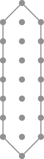
Figure 2. The polygons $P_{3},Q_{3}$ and $P_{3}+Q_{3}$.

Since the Minkowski sum $P_{n}+Q_{n}$ is a hexagon, there are only six directional resultants appearing in (4.4). Choosing the inner normal vectors $(1,0)$ or $(-1,0)$, the corresponding directional resultant is the classical resultant of two univariate polynomials of degree $n$. The other four inner normal vectors yield directional resultants that are monomials.

6.7. Example: Non-Chasles configuration and non rational extra point map

Let $A$ be the set of lattice points in the triangle in ${\mathbb{R}}^{2}$ with vertices $(0,0),(1,2),(3,1)$, with two interior points $(1,1),(2,1)$, so that $A$ has 5 points, and ${\rm vol}(A)=5$; $A$ is not a Chasles configuration because three zeros, in general, induce two more zeros. Our goal here is to show that the map that assigns the two new zeros to the original three is not rational. It suffices to fix two of the original zeros and make the third variable, and show that the coordinates of the new points involve square roots of the coordinates of the third.

Let us specify that our three points are $(1,1)$, $(2,4)$ and $(t,t^{2})$, $t\neq 0,1,2$. There is a two dimensional family of polynomials supported on $A$ that vanish on these three points. The following is a choice of basis for this vector space.

$$F_{1}(x,y) =xy^{2}-x^{3}y=xy(y-x^{2});$$

$$F_{2}(x,y) =-8t^{3}+(8+12t+14t^{2}+15t^{3})xy$$

$$\qquad-(12+18t+21t^{2}+7t^{3})x^{2}y+(4+6t+7t^{2})x^{3}y.$$

To find additional common zeros, we note that $F_{2}(x_{0},y_{0})\neq 0$ for $x_{0}y_{0}=0$, and so any zero also lies on $y_{0}=x_{0}^{2}$. A computation shows that

$$F_{2}(x_{0},x_{0}^{2})=(x_{0}-1)(x_{0}-2)(x_{0}-t)q(x_{0});\text{ where }q(x_{0})=(4+6t+7t^{2})x_{0}^{2}+(4t+6t^{2})x_{0}+4t^{2}.$$

Since the discriminant of $q$ is $-4t^{2}(12+12t+19t^{2})$, which is not a square, the values for $x_{0}$ involves square roots of polynomials involving $t$ and hence is not a rational function of $\{1,1,2,4,t,t^{2}\}$.

References

• [B75] David Bernstein, The number of roots of a system of equations, Funkcional. Anal. i Priložen., 9 (1975), 1–4.
• [B06] Robert Bix, Conics and cubics, Second ed., Undergraduate Texts in Mathematics, Springer, New York, 2006, A concrete introduction to algebraic curves.
• [CDS98] Eduardo Cattani, Alicia Dickenstein and Bernd Sturmfels, Residues and resultants, J. Math. Sci. Univ.Tokyo 5 (1998), 119-–148.
• [CLR87] Man-Duen Choi, Tsit-Yuen Lam, Bruce Reznick Even symmetric sextics, Math. Z., 195 (1987), 559–580, (MR88j:11019).
• [DS15] Carlos D’Andrea and Martín Sombra, A Poisson formula for the sparse resultant, Proc. London Math. Soc. (3) 110 (2015), 932-–964.
• [E10] Alexander Esterov, Newton polyhedra of discriminants of projections, Discrete Comput. Geom. 44 (2010), 96-–148.
• [EGH96] David Eisenbud, Mark Green, and Joe Harris, Cayley-Bacharach theorems and conjectures, Bull. Amer. Math. Soc. (N.S.) 33 (1996), no. 3, 295–324.
• [M2] Daniel R. Grayson and Michael E. Stillman, Macaulay2, a software system for research in algebraic geometry Available at http://www.math.uiuc.edu/Macaulay2/.
• [H83] Douglas Hensley, Lattice vertex polytopes with interior lattice points, Pacific J. Math., 105, (1983), no. 1, 183–191.
• [H1888] David Hilbert, Über die Darstellung definiter Formen als Summe von Formenquadraten, Math. Ann. 32 (1888), 342–350; see Ges. Abh. 2, 154–161, Springer, Berlin, 1933, reprinted by Chelsea, New York, 1981.
• [K97] Askold Khovanskii, Newton polyhedra, a new formula for mixed volume, product of roots of a system of equations, The Arnoldfest (Toronto, ON, 1997), Fields Inst. Commun., vol. 24, Amer. Math. Soc., 1999, pp. 325–-364.
• [K76] Anatoli Kouchnirenko, Polyèdres de Newton et nombres de Milnor. (French) Invent. Math. 32 (1976), no. 1, 1-–31.
• [KS97] Maximilian Kreuzer and Harald Skarke, On the classification of reflexive polyhedra Comm. Math. Phys. 185 (1997), no. 2, 495–-508.
• [KS98] Maximilian Kreuzer and Harald Skarke, Classification of reflexive polyhedra in three dimensions, Adv. Theor. Math. Phys. 2 (1998), no. 4, 853–-871.
• [KS00] Maximilian Kreuzer and Harald Skarke, Complete classification of reflexive polyhedra in four dimensions, Adv. Theor. Math. Phys. 4 (2000), no. 6, 1209-–1230.
• [PS93] Paul Pedersen and Bernd Sturmfels, Product formulas for resultants and Chow forms, Math. Z. 214 (1993), 377-–396.
• [PSV11] Daniel Plaumann, Bernd Sturmfels and Cynthia Vinzant, Quartic curves and their bitangents, J. Symbolic Comput. 46 (2011), no. 6, 712–-733.
• [RRS15] Qingchun Ren, Jürgen Richter-Gebert and Bernd Sturmfels, Cayley–Bacharach formulas, Amer. Math. Monthly 122 (2015), no. 9, 845–854.
• [R00] Bruce Reznick, Some concrete aspects of Hilbert’s 17th Problem, Contemp. Math., 253 (2000), 251–272.
• [R07] Bruce Reznick, On Hilbert’s construction of positive polynomials, arXiv:0707.2156.
• [R69] Raphael M. Robinson, Some definite polynomials which are not sums of squares of real polynomials, Izdat. “Nauka” Sibirsk. Otdel. Novosibirsk, (1973) pp. 264–282, (Selected questions of algebra and logic (a collection dedicated to the memory of A. I. Mal’cev), abstract in Notices AMS, 16 (1969), p. 554.
• [R97] J. Maurice Rojas, Toric laminations, sparse generalized characteristic polynomials, and a refinement of Hilbert’s tenth problem, Foundations of computational mathematics (Rio de Janeiro, 1997), 369–-381, Springer, Berlin, 1997.
• [S76] P. R. Scott, On convex lattice polygons, Bull. Austral. Math. Soc., 15 (1976), 395–399.
• [S94] Bernd Sturmfels, On the Newton Polytope of the Resultant, J. Algebraic Combin. 3 (1994), 207–236.