Equidistribution of critical points of the multipliers in the quadratic family

Abstract.

A parameter $c_{0}\in\mathbb{C}$ in the family of quadratic polynomials $f_{c}(z)=z^{2}+c$ is a critical point of a period $n$ multiplier, if the map $f_{c_{0}}$ has a periodic orbit of period $n$, whose multiplier, viewed as a locally analytic function of $c$, has a vanishing derivative at $c=c_{0}$. We prove that all critical points of period $n$ multipliers equidistribute on the boundary of the Mandelbrot set, as $n\to\infty$.

1. Introduction

Consider the family of quadratic polynomials

$$f_{c}(z)=z^{2}+c,\qquad c\in\mathbb{C}.$$

We say that a parameter $c_{0}\in\mathbb{C}$ is a critical point of a period $n$ multiplier, if the map $f_{c_{0}}$ has a periodic orbit of period $n$, whose multiplier, viewed as a locally analytic function of $c$, has a vanishing derivative at $c=c_{0}$.

The study of these critical points is motivated by the following observation: the argument of quasiconformal surgery implies that appropriate inverse branches of the multipliers of periodic orbits, viewed as analytic functions of the parameter $c$, are Riemann mappings of the corresponding hyperbolic components of the Mandelbrot set [Milnor_hyper]. Possible existence of analytic extensions of these Riemann mappings to larger domains might allow to estimate the geometry of the hyperbolic components [Levin_2009, Levin_2011]. Critical values of the multipliers are the only obstructions for existence of these analytic extensions.

For each $n\in\mathbb{N}$, let $X_{n}$ be the set of all parameters $c\in\mathbb{C}$ that are critical points of a period $n$ multiplier (counted with multiplicities). Let $\mathbb{M}\subset\mathbb{C}$ denote the Mandelbrot set and let $\mu_{\mathrm{bif}}$ be its equilibrium measure (or the bifurcation measure of the quadratic family $\{f_{c}\}$).

Our first main result is the following:

Theorem A.

The sequence of probability measures

$$\nu_{n}=\frac{1}{\#X_{n}}\sum_{x\in X_{n}}\delta_{x}$$

converges to the equilibrium measure $\mu_{\mathrm{bif}}$ in the weak sense of measures on $\mathbb{C}$, as $n\to\infty$.

In particular, Theorem A gives a positive answer to the question, stated in [Belova_Gorbovickis].

We note that Theorem A is a partial case of a more general result that we prove in this paper. A precise statement of this more general result will be given in the next section (c.f.  Theorem 2.5).

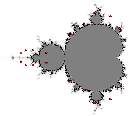
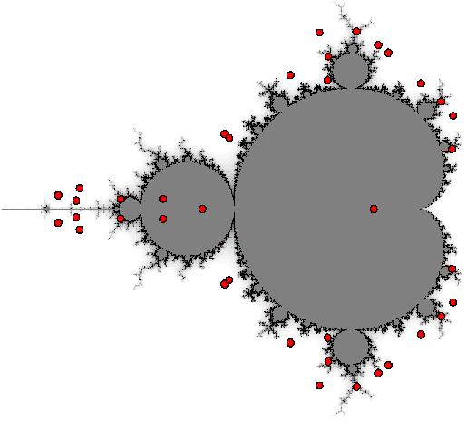
(a)	(b)
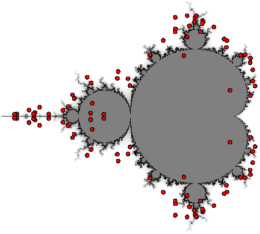
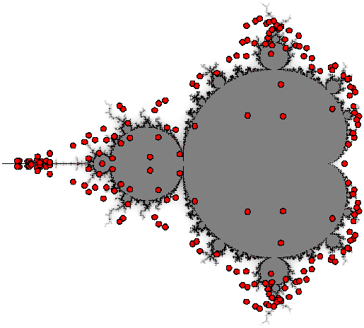
(c)	(d)

Figure 1. Critical points of the multipliers: (a) period 5; (b) period 6; (c) period 7; (d) period 8.

Equidistribution results in the parameter plane have attracted a lot of attention: starting from the results for critically periodic parameters of period $n$ [Levin], to more recent results for parameters with a prescribed multiplier  [Bassanelli_Berteloot, Buff_Gauthier] and Misiurewicz points [FRL, DF, Gauthier_Vigny_2019]. It is important to note that for all of the above mentioned classes of points in the quadratic family, their accumulation sets coincide with the support of $\mu_{\mathrm{bif}}$, i.e., the boundary of the Mandelbrot set. The latter is not the case for critical points of the multipliers. In particular, we prove the following theorem.

Theorem B.

For every $n_{0}\in\mathbb{N}$ and $c\in X_{n_{0}}\setminus\mathbb{M}$, there exists a sequence $\{c_{n}\}_{n=3}^{\infty}$, such that $c_{n}\in X_{n}$, for any $n\geq 3$, and

$$\lim_{n\to\infty}c_{n}=c.$$

Theorem B can be loosely interpreted as follows: fix an arbitrary $n_{0}\in\mathbb{N}$. Then for any sufficiently large $n\in\mathbb{N}$, the set $X_{n}\setminus\mathbb{M}$ contains a “distorted” copy of $X_{n_{0}}\setminus\mathbb{M}$ as a subset. The larger is $n$, the closer is this copy to the original set $X_{n_{0}}\setminus\mathbb{M}$ (in Hausdorff metric).

We remark that the sequence of parameters $c_{n}$ in Theorem B starts from $n=3$, because the sets $X_{1}$ and $X_{2}$ are empty. We also note that according to the numerical computations in [Belova_Gorbovickis], the sets $X_{n}\setminus\mathbb{M}$ are nonempty, for all $n=3,4,\dots,10$, so Theorem B implies that the sets $X_{n}\setminus\mathbb{M}$ are nonempty for all sufficiently large $n$.

Let $\mathcal{X}$ be the set of all accumulation points of the sets $X_{n}$, i.e.

$$\mathcal{X}:=\bigcap_{k=3}^{\infty}\left(\,\overline{\bigcup_{n=k}^{\infty}X_{n}}\,\right).$$

The above discussion suggests that this set might have nontrivial geometry. In particular, Theorem B implies the following inclusion:

$$\overline{\bigcup_{n=3}^{\infty}(X_{n}\setminus\mathbb{M})}\subset\mathcal{X}.$$

We also know from [Belova_Gorbovickis] and [Reinke] that $0\in\mathcal{X}$. In an upcoming paper we will study some further geometric properties of the set $\mathcal{X}$.

The structure of the paper is as follows: in Section 2 we give the necessary basic definitions and state our main results in a more precise form. In Section 3 we describe the derivatives of the multipliers as algebraic functions (i.e., roots of polynomial equations). This allows us to explicitly compute potentials of the measures $\nu_{n}$. In Section 4 we give a proof of Theorem 2.5, a more general version of Theorem A, modulo Lemma 4.2 that states convergence of potentials in the complement of the Mandelbrot set. A key tool in our proof is Lemma 4.1 that was proved by Buff and Gauthier in [Buff_Gauthier]. Sections 5 and 6 are devoted to the study of the multipliers of periodic orbits viewed as functions of the parameter $c\in\mathbb{C}\setminus\mathbb{M}$ in the complement of the Mandelbrot set. In this case it turns out to be more natural to study the degree $n$ roots of the multipliers, where $n$ is the period of the corresponding periodic orbits. In Section 5 we use the Ergodic Theorem to prove that as $n\to\infty$, the roots of the multipliers of the majority of periodic orbits behave as twice the square root of the uniformizing coordinate of $\mathbb{C}\setminus\mathbb{M}$ onto $\mathbb{C}\setminus\overline{\mathbb{D}}$ (c.f., Theorem 5.5). At the same time, we construct examples of sequences of periodic orbits, whose roots of the multipliers behave differently. This way we obtain a proof of Theorem B. Finally, in Section 6 we use the results of Section 5 to prove Lemma 4.2, this way, completing the proof of Theorem 2.5.

2. Statement of results

A point $z\in\mathbb{C}$ is a periodic point of the polynomial $f_{c}$, if there exists a positive integer $n\in\mathbb{N}$, such that $f_{c}^{\circ n}(z)=z$. The smallest such $n$ is called the period of the periodic point $z$.

Given $n$, let the period $n$ curve $\mathrm{Per}_{n}\subset\mathbb{C}\times\mathbb{C}$ be the closure of the locus of points $(c,z)$ such that $z$ is a periodic point of $f_{c}$ of period $n$. Observe that each pair $(c,z)\in\mathrm{Per}_{n}$ determines a periodic orbit

$$z=z_{0}\mapsto z_{1}\mapsto\cdots\mapsto z_{n}=z_{0}$$

of either period $n$ or of a smaller period that divides $n$ (see  [Milnor_external_rays] for more details).

Let $\mathbb{Z}_{n}$ denote the cyclic group of order $n$. This group acts on $\mathrm{Per}_{n}$ by cyclicly permuting points of the same periodic orbits for each fixed value of $c$. Then the factor space $\mathrm{Per}_{n}/\mathbb{Z}_{n}$ consists of pairs $(c,\mathcal{O})$ such that $\mathcal{O}$ is a periodic orbit of $f_{c}$.

Let $\tilde{\rho}_{n}:\mathrm{Per}_{n}\to\mathbb{C}$ be the map defined by

$$\tilde{\rho}_{n}\colon(c,z)\mapsto\frac{\partial f^{\circ n}_{c}}{\partial z}(z)=2^{n}z_{1}\cdots z_{n}.$$

Observe that $\tilde{\rho}_{n}(c,z)$ is the multiplier of a periodic point $z$, whenever $z$ has period $n$. Otherwise, if a point $z$ has period $n/r$, where $r>1$ is some divisor of $n$, then $\tilde{\rho}_{n}(c,z)$ is the $r$-th power of the multiplier of $z$. Furthermore, if $z_{1}$ and $z_{2}$ belong to the same periodic orbit of $f_{c}$, then $\tilde{\rho}_{n}(c,z_{1})=\tilde{\rho}_{n}(c,z_{2})$, hence the map $\tilde{\rho}_{n}$ projects to a well defined map

$$\rho_{n}\colon\mathrm{Per}_{n}/\mathbb{Z}_{n}\to\mathbb{C}$$

that assigns to each pair $(c,\mathcal{O})$ the multiplier of the periodic orbit $\mathcal{O}$. Note that according to [Milnor_external_rays], the space $\mathrm{Per}_{n}/\mathbb{Z}_{n}$ (as well as $\mathrm{Per}_{n}$) has a structure of a smooth algebraic curve, and both $\rho_{n}$ and $\tilde{\rho}_{n}$ are proper algebraic maps.

It follows from the Implicit Function Theorem that if a point $(c,\mathcal{O})\in\mathrm{Per}_{n}/\mathbb{Z}_{n}$ is such that the periodic orbit $\mathcal{O}$ has period less than $n$, then $\rho_{n}(c,\mathcal{O})=1$.

Definition 2.1.

A point $(c,z)\in\mathrm{Per}_{n}$ and its projection $(c,\mathcal{O})\in\mathrm{Per}_{n}/\mathbb{Z}_{n}$ are called parabolic, if $\rho_{n}(c,\mathcal{O})=1$. A parabolic point $(c,z)\in\mathrm{Per}_{n}$ and its projection $(c,\mathcal{O})\in\mathrm{Per}_{n}/\mathbb{Z}_{n}$ are called primitive parabolic, if the period of the point $z$ is equal to $n$. Otherwise, a parabolic point is called satellite. The set of all primitive parabolic points of $\mathrm{Per}_{n}/\mathbb{Z}_{n}$ will be denoted by $\mathcal{P}_{n}\subset\mathrm{Per}_{n}/\mathbb{Z}_{n}$.

Remark 2.2.

Alternatively, one usually defines parabolic parameters $c$ as those, for which there exists a periodic orbit $\mathcal{O}$ of $f_{c}$ with a root of unity as its multiplier. Comparing this with Definition 2.1, we note that for every parabolic parameter $c\in\mathbb{C}$ (in the sense of the standard definition), there exist $n\in\mathbb{N}$ and $z\in\mathbb{C}$, such that $(c,z)\in\mathrm{Per}_{n}$, and the point $(c,z)\in\mathrm{Per}_{n}$ is parabolic in the sense of Definition 2.1.

It is well known that the coordinate $c$ can serve as a local chart on $\mathrm{Per}_{n}/\mathbb{Z}_{n}$ at all points $(c,\mathcal{O})$ that are not primitive parabolic (c.f. [Milnor_external_rays]). Hence, outside of these points one can consider the derivative of the multiplier map $\rho_{n}$ with respect to $c$. Thus, we let the map

$$\sigma_{n}\colon(\mathrm{Per}_{n}/\mathbb{Z}_{n})\setminus\mathcal{P}_{n}\to\mathbb{C}$$

be defined by the relation

(1) $$\sigma_{n}:=\frac{d}{dc}\rho_{n}.$$

In particular, for every non-parabolic point $(c_{0},\mathcal{O})\in\mathrm{Per}_{n}/\mathbb{Z}_{n}$ that is the projection of a point $(c_{0},z_{0})\in\mathrm{Per}_{n}$, one can define a locally analytic function $z(c)\in\mathbb{C}$, such that $z(c_{0})=z_{0}$ and $(c,z(c))\in\mathrm{Per}_{n}$, for all $c$ in a neighborhood of $c_{0}$. Then (1) implies that

$$\sigma_{n}(c_{0},\mathcal{O})=h^{\prime}(c_{0}),\quad\text{where}\quad h(c)=\tilde{\rho}_{n}(c,z(c)).$$

Remark 2.3.

It follows from Lemma 4.5 from [Milnor_external_rays] that if $(c_{0},\mathcal{O}_{0})\in\mathcal{P}_{n}$ is a primitive parabolic point, then $|\sigma_{n}(c,\mathcal{O})|\sim 1/\sqrt{|c-c_{0}|}$, as $(c,\mathcal{O})\to(c_{0},\mathcal{O}_{0})$.

Definition 2.4.

For any $s\in\mathbb{C}$ and any $n\in\mathbb{N}$, let $Y_{s,n}\subset\mathrm{Per}_{n}/\mathbb{Z}_{n}$ be the set of all solutions of the equation $\sigma_{n}(c,\mathcal{O})=s$. For any solution of this equation $(c,\mathcal{O})\in Y_{s,n}$, let $\tilde{m}_{s,n}(c,\mathcal{O})$ be its multiplicity. Finally, let $X_{s,n}\subset\mathbb{C}$ be the projection of the set $Y_{s,n}$ onto the first coordinate, and for any $c\in X_{s,n}$, define $m_{s,n}(c)$ as

$$m_{s,n}(c):=\sum_{\mathcal{O}\mid(c,\mathcal{O})\in Y_{s,n}}\tilde{m}_{s,n}(c,\mathcal{O}),$$

where the summation goes over all periodic orbits $\mathcal{O}$, such that $(c,\mathcal{O})\in Y_{s,n}$.

We will show in Lemma 3.3 that for every $n\geq 3$, the number $\sum_{c\in X_{s,n}}m_{s,n}(c)$ is independent of the choice of $s\in\mathbb{C}$. Hence, for every $n\geq 3$ we define

(2) $$M_{n}:=\sum_{c\in X_{s,n}}m_{s,n}(c).$$

For $c\in\mathbb{C}$, let $\delta_{c}$ be the delta measure at the point $c$, and for every $n\geq 3$, and $s\in\mathbb{C}$, consider the probability measure

$$\nu_{s,n}:=\frac{1}{M_{n}}\sum_{c\in X_{s,n}}m_{s,n}(c)\delta_{c}.$$

For $c\in\mathbb{C}$, the Green’s function $G_{c}\colon\mathbb{C}\to[0,+\infty)$ of the polynomial $f_{c}$ is given by

$$G_{c}(z):=\lim_{n\to+\infty}\max\{2^{-n}\log|f_{c}^{\circ n}(z)|,\,\,0\},$$

and the Green’s function $G_{\mathbb{M}}\colon\mathbb{C}\to[0,+\infty)$ of the Mandelbrot set $\mathbb{M}$ satisfies

$$G_{\mathbb{M}}(c):=G_{c}(c)$$

(see [Douady_Hubbard] for details). Finally, the bifurcation measure $\mu_{\mathrm{bif}}$ is defined by

$$\mu_{\mathrm{bif}}:=\Delta G_{\mathbb{M}},$$

where $\Delta$ is the generalized Laplacian.

A more general version of our first main result (Theorem A) is the following:

Theorem 2.5.

For every sequence of complex numbers $\{s_{n}\}_{n\in\mathbb{N}}$, such that

(3) $$\limsup_{n\to+\infty}\frac{1}{n}\log|s_{n}|\leq\log 2,$$

the sequence of measures $\{\nu_{s_{n},n}\}_{n\in\mathbb{N}}$ converges to $\mu_{\mathrm{bif}}$ in the weak sense of measures on $\mathbb{C}$.

3. Derivatives of the multipliers as algebraic functions

For every integer $n\geq 1$, let $\tilde{\mathcal{P}}_{n}\subset\mathbb{C}$ be the projection of the set of all primitive parabolic points $\mathcal{P}_{n}$ onto the first coordinate. That is,

$$\tilde{\mathcal{P}}_{n}:=\{c\in\mathbb{C}\mid(c,\mathcal{O})\in\mathcal{P}_{n},\text{ for some periodic orbit }\mathcal{O}\}.$$

Remark 3.1.

For $n=1$ and $n=2$, the sets $\mathcal{P}_{n}$ and $\tilde{\mathcal{P}}_{n}$ are empty.

Consider the functions $\tilde{S}_{n}\colon(\mathbb{C}\setminus\tilde{\mathcal{P}}_{n})\times\mathbb{C}\to\mathbb{C}$ defined by the formula

(4) $$\tilde{S}_{n}(c,s):=\prod_{\mathcal{O}\mid(c,\mathcal{O})\in\mathrm{Per}_{n}/\mathbb{Z}_{n}}(s-\sigma_{n}(c,\mathcal{O})),$$

where the product is taken over all periodic orbits $\mathcal{O}$, such that $(c,\mathcal{O})\in\mathrm{Per}_{n}/\mathbb{Z}_{n}$. Also consider the polynomials $C_{n}\colon\mathbb{C}\to\mathbb{C}$ defined by the formula

$$C_{n}(c):=\prod_{\tilde{c}\in\tilde{\mathcal{P}}_{n}}(c-\tilde{c}).$$

One of the main results of this section is the following lemma:

Lemma 3.2.

For any $n\geq 3$, define

$$S_{n}(c,s):=C_{n}(c)\tilde{S}_{n}(c,s).$$

Then the function $S_{n}$ is a polynomial in $c$ and $s$, satisfying the property that $S_{n}(c,s)=0$ for a pair $(c,s)\in\mathbb{C}^{2}$, if and only if $s=\sigma_{n}(c,\mathcal{O})$, for some $(c,\mathcal{O})\in\mathrm{Per}_{n}/\mathbb{Z}_{n}$ (taking into the account multiplicities).

Proof.

First, it follows from (4) that for every $c\in\mathbb{C}\setminus\tilde{\mathcal{P}}_{n}$, the functions $\tilde{S}_{n}(c,s)$ and hence the functions $S_{n}(c,s)$ are polynomials in $s$.

Next, we observe that $\tilde{S}_{n}(c,s)$ is analytic in $c\in\mathbb{C}\setminus\tilde{\mathcal{P}}_{n}$. Furthermore, according to the Fatou-Shishikura inequality, for every $c_{0}\in\tilde{\mathcal{P}}_{n}$, there is exactly one parabolic point $(c_{0},\mathcal{O}_{0})\in\mathrm{Per}_{n}/\mathbb{Z}_{n}$ and the multiplicity of this point is equal to $2$ (i.e., when $c_{0}$ is perturbed to some nearby value $c\in\mathbb{C}$, the periodic orbit $\mathcal{O}_{0}$ splits into exactly two periodic orbits of period $n$). Now it follows from (4) and Remark 2.3 that for every $s\in\mathbb{C}$, the function $S(c)=\tilde{S}_{n}(c,s)$ is meromorphic in $\mathbb{C}$ with simple poles at each point from the set $\tilde{\mathcal{P}}_{n}$.

Finally, we note that according to [Buff_Gauthier], $|\rho_{n}(c,\mathcal{O})|\sim|4c|^{\frac{n}{2}}$ as $c\to\infty$, hence, for $n\geq 3$ we have $\sigma_{n}(c,\mathcal{O})\to\infty$ as $c\to\infty$. Thus, for every $s\in\mathbb{C}$, the function $S(c)=\tilde{S}_{n}(c,s)$ cannot have an essential singularity at infinity, hence is a rational function. Multiplication by $C_{n}(c)$ eliminates all simple poles at the points of the set $\tilde{\mathcal{P}}_{n}$, so the product $C_{n}(c)\tilde{S}_{n}(c,s)$ extends to a polynomial in $\mathbb{C}^{2}$.

The second part of the lemma follows immediately from the construction of the polynomial $S_{n}$. ∎

For every $n\geq 3$, let $\deg_{c}S_{n}$ denote the highest degree of $S_{n}$ as a polynomial in $c$ with coefficients from the polynomial ring $\mathbb{C}[s]$.

Lemma 3.3.

For every $n\geq 3$, we have

$$\deg_{c}S_{n}=M_{n},$$

where $M_{n}$ is defined in (2) as the number of solutions $(c,\mathcal{O})$ of the equation $\sigma_{n}(c,\mathcal{O})=s$ (counted with multiplicity). In particular, this shows that $M_{n}$ is independent of $s\in\mathbb{C}$.

Proof.

For any $s\in\mathbb{C}$, define $T_{n,s}(c):=S_{n}(c,s)$. Then $T_{n,s}$ is a polynomial in variable $c$. It follows from Lemma 3.2 that for any $s\in\mathbb{C}$, we have

$$\sum_{c\in X_{s,n}}m_{s,n}(c)=\deg T_{n,s}.$$

We complete the proof by observing that $\deg T_{n,s}=\deg_{c}S_{n}$, for any $s\in\mathbb{C}$. The latter follows from the fact that according to [Buff_Gauthier], $|\rho_{n}(c,\mathcal{O})|\sim|4c|^{\frac{n}{2}}$, as $c\to\infty$, hence, for $n\geq 3$ we have $\sigma_{n}(c,\mathcal{O})\to\infty$ as $c\to\infty$, which implies that the coefficient in front of the highest degree term in $c$ of the polynomial $S_{n}$ is a constant, independent of $s$. ∎

The next lemma summarizes the asymptotic behavior of the degrees of the polynomials $S_{n}$.

Lemma 3.4.

The following limit holds:

$$\lim_{n\to+\infty}2^{-n}(\deg_{c}S_{n})=1.$$

Proof.

For every $n\in\mathbb{N}$, let $\nu(n)$ be the number of periodic points of period $n$ for a generic quadratic polynomial $f_{c}$. The function $\nu(n)$ can be computed inductively by the formulas

(5) $$2^{n}=\sum_{r|n}\nu(r)\qquad\text{or}\qquad\nu(n)=\sum_{r|n}\mu(n/r)2^{r},$$

where the summation goes over all divisors $r\geq 1$ of $n$, and $\mu(n/r)\in\{\pm 1,0\}$ is the Möbius function.

It is easy to see from the second formula that

$$\nu(n)\geq 2^{n}-\sum_{0\leq j\leq n/2}2^{j}\geq 2^{n}-2^{\frac{n}{2}+1}.$$

On the other hand, since $\nu(n)\leq 2^{n}$, it follows that

$$\lim_{n\to\infty}2^{-n}\nu(n)=1.$$

It was shown in [Belova_Gorbovickis] that $\deg_{c}S_{n}$ can be expressed in terms of the function $\nu(n)$ by the formula

$$\deg_{c}S_{n}=\nu(n)-\frac{\nu(n)}{n}-\sum_{n=rp,p<n}\nu(p)\phi(r),$$

where $\phi(r)$ is the number of positive integers that are smaller than $r$ and relatively prime with $r$. Since

(6) $$\sum_{n=rp,p<n}\nu(p)\phi(r)\leq\sum_{n=rp,p<n}2^{n/2}n\leq\frac{n}{2}\cdot 2^{n/2}n=2^{\frac{n}{2}-1}n^{2},$$

it follows that

$$\lim_{n\to\infty}2^{-n}\sum_{n=rp,p<n}\nu(p)\phi(r)=0,$$

hence

$$\lim_{n\to+\infty}2^{-n}(\deg_{c}S_{n})=\lim_{n\to+\infty}2^{-n}\left[\nu(n)-\frac{\nu(n)}{n}\right]=1.$$

∎

4. Proof of Theorem 2.5

In this section we give a proof of Theorem 2.5 modulo the auxiliary lemmas stated below. The strategy of the proof follows the one from [Buff_Gauthier].

Consider the subharmonic function $v\colon\mathbb{C}\to[0,+\infty)$ defined by

$$v:=G_{\mathbb{M}}+\log 2.$$

The following lemma was proven in [Buff_Gauthier].

Lemma 4.1 ([Buff_Gauthier]).

Any subharmonic function $u\colon\mathbb{C}\to[-\infty,+\infty)$ which coincides with $v$ outside the Mandelbrot set $\mathbb{M}$, coincides with $v$ everywhere in $\mathbb{C}$.

Now for every $n\in\mathbb{N}$ and $s\in\mathbb{C}$, we define

(7) $$u_{s,n}(c):=(\deg_{c}S_{n})^{-1}\log|S_{n}(c,s)|.$$

Then it follows from Lemma 3.2 and Lemma 3.3 that $u_{s,n}$ is a potential of the measure $\nu_{s,n}$, which means that

$$\nu_{s,n}=\Delta u_{s,n}.$$

The following lemma is crucial for the proof of Theorem 2.5.

Lemma 4.2.

For every sequence of complex numbers $\{s_{n}\}_{n\in\mathbb{N}}$, satisfying (3), the sequence of subharmonic functions $\{u_{s_{n},n}\}_{n\in\mathbb{N}}$ converges to $v$ in $L^{1}_{\mathrm{loc}}$ on the set $\mathbb{C}\setminus\mathbb{M}$.

The proof of Lemma 4.2 will occupy most of the remaining part of the paper. Note that in the special case of Theorem A, namely, the case when $s_{n}=0$ for every $n\in\mathbb{N}$, we can simplify the proof of Lemma 4.2 (see Remark 5.4).

Now we give a proof of Theorem 2.5 modulo Lemma 4.2.

Proof of Theorem 2.5.

It follows from Lemma 4.2 and Prokhorov’s Theorem that the sequence of measures $\nu_{n}:=\nu_{{s_{n}},n}$ is sequentially relatively compact with respect to the weak convergence. Let $\nu$ be a probability measure that is a limit point of the sequence $\{\nu_{n}\}_{n\in\mathbb{N}}$. Then there exists a subsequence $\{n_{k}\}$, such that $\nu_{n_{k}}\to\nu$ in the weak sense of measures on $\mathbb{C}$, as $k\to\infty$, and the sequence $\{u_{s_{n_{k}},n_{k}}\}$ converges in $L^{1}_{\mathrm{loc}}$ to a subharmonic function $u$ on $\mathbb{C}$, satisfying

$$\Delta u=\nu.$$

Furthermore, it follows from Lemma 4.2 that $u(c)=v(c)$, for all $c\in\mathbb{C}\setminus\mathbb{M}$, hence Lemma 4.1 implies that

$$u\equiv v\qquad\text{on}\quad\mathbb{C}.$$

Thus, we conclude that the sequence of measures $\nu_{n}$ has only one limit point $\nu$, hence the sequence converges to $\nu$, where

$$\nu=\Delta v=\Delta G_{\mathbb{M}}=\mu_{\mathrm{bif}}.$$

∎

5. Roots of the multipliers and the ergodic theorem

The aim of this section is to study the behavior of the multipliers of the maps $f_{c}$, when the parameter $c$ lies outside of the Mandelbrot set $\mathbb{M}$ and the period $n$ of the periodic orbits increases to infinity. It turns out to be quite natural to look at the degree $n$ roots of the multipliers. Precise definitions are given in the following subsection.

5.1. Roots of the multipliers outside the Mandelbrot set

First, we summarize some well-known facts about the dynamics of $f_{c}$, when $c\in\mathbb{C}\setminus\mathbb{M}$. More details can be found in [Blanchard_Devaney_Keen].

First, if $c\in\mathbb{C}\setminus\mathbb{M}$, then the Julia set $J_{c}$ of $f_{c}$ is a Cantor set and $0\not\in J_{c}$. The dynamics of $f_{c}$ on the Julia set $J_{c}$ is topologically conjugate to the Bernoulli shift on 2 symbols. Furthermore, the periodic points of $f_{c}$ move locally holomorphically with respect to the parameter $c$ when the latter varies outside of the Mandelbrot set $\mathbb{M}$, hence, by $\lambda$-Lemma [Lyubich, ManeSadSullivan], this holomorphic motion extends to a local holomorphic motion of the whole Julia set $J_{c}$. Since $\mathbb{M}$ is connected and simply connected, there exists a unique nontrivial monodromy loop in $\mathbb{C}\setminus\mathbb{M}$, namely, the loop that goes around $\mathbb{M}$ once. If we start with $c\in(1/4,+\infty)$ and make a loop around $\mathbb{M}$ (say, in the counterclockwise direction), then each point of $J_{c}$ comes back to its complex conjugateunder the above holomorphic motion. Going around this loop twice, brings every point of $J_{c}$ back to itself. This makes it natural to consider a degree 2 covering of $\mathbb{C}\setminus\mathbb{M}$.

More specifically, let

$$\phi_{\mathbb{M}}\colon\mathbb{C}\setminus\mathbb{M}\to\mathbb{C}\setminus\overline{\mathbb{D}}$$

be the conformal diffeomorphism of $\mathbb{C}\setminus\mathbb{M}$ onto $\mathbb{C}\setminus\overline{\mathbb{D}}$ that sends the real ray $(1/4,+\infty)$ to $(1,+\infty)$. For $\lambda\in\mathbb{C}\setminus\overline{\mathbb{D}}$, set

(8) $$\mathbf{c}(\lambda):=\phi_{\mathbb{M}}^{-1}(\lambda^{2}).$$

Then $\mathbf{c}\colon\mathbb{C}\setminus\overline{\mathbb{D}}\to\mathbb{C}\setminus\mathbb{M}$ is a covering map of degree 2. In addition to that, for every $\lambda\in\mathbb{C}\setminus\overline{\mathbb{D}}$, we have the following relation that will be useful in Section 6:

(9) $$\log|\lambda|=\frac{1}{2}G_{\mathbb{M}}(\mathbf{c}(\lambda)).$$

Let $\Omega:=\{0,1\}^{\mathbb{N}}$ be the space of all infinite binary sequences with the standard metric $d\colon\Omega\times\Omega\to\mathbb{R}^{+}$ defined as follows: if $\mathbf{w}_{1}=(\omega_{0}^{1},\omega_{1}^{1},\omega_{2}^{1},\ldots)\in\Omega$ and $\mathbf{w}_{2}=(\omega_{0}^{2},\omega_{1}^{2},\omega_{2}^{2},\ldots)\in\Omega$, then

$$d(\mathbf{w}_{1},\mathbf{w}_{2})=2^{-k},$$

where $k\in\{0\}\cup\mathbb{N}$ is the smallest index, for which $\omega_{k}^{1}\neq\omega_{k}^{2}$. Let $\sigma\colon\Omega\to\Omega$ be the left shift. An element $\mathbf{w}=(\omega_{0},\omega_{1},\omega_{2},\dots)\in\Omega$ is called an itinerary. There exists a uniquely defined one parameter family of maps

$$\psi_{\lambda}\colon\Omega\to\mathbb{C},\qquad\lambda\in\mathbb{C}\setminus\overline{\mathbb{D}}$$

such that the following conditions hold simultaneously:

• for any $\lambda\in\mathbb{C}\setminus\overline{\mathbb{D}}$, the map $\psi_{\lambda}$ is a homeomorphism between $\Omega$ and $J_{\mathbf{c}(\lambda)}$, conjugating $\sigma$ to $f_{\mathbf{c}(\lambda)}$:

  $$\psi_{\lambda}\circ\sigma=f_{\mathbf{c}(\lambda)}\circ\psi_{\lambda};$$

• for each $\mathbf{w}\in\Omega$, the point $\psi_{\lambda}(\mathbf{w})$ depends analytically on $\lambda\in\mathbb{C}\setminus\overline{\mathbb{D}}$;

• for each $\lambda\in(1,+\infty)$ and $\mathbf{w}=(\omega_{0},\omega_{1},\omega_{2},\dots)\in\Omega$, the point $\psi_{\lambda}(\mathbf{w})$ is in the upper half-plane, if and only if $\omega_{0}=0$.

For further convenience in notation we define a function $\psi\colon\mathbb{C}\setminus\overline{\mathbb{D}}\times\Omega\to\mathbb{C}$ by the relation

$$\psi(\lambda,\mathbf{w})=\psi_{\lambda}(\mathbf{w}).$$

Then, for each $\mathbf{w}\in\Omega$ we define the map $\psi_{\mathbf{w}}\colon\mathbb{C}\setminus\overline{\mathbb{D}}\to\mathbb{C}$ according to the relation

$$\psi_{\mathbf{w}}(\lambda)=\psi(\lambda,\mathbf{w}).$$

It follows from our construction that for each $\mathbf{w}=(\omega_{0},\omega_{1},\omega_{2},\dots)\in\Omega$, the map $\psi_{\mathbf{w}}$ is holomorphic. Furthermore,

(10) $$\psi_{\mathbf{w}}(\lambda)\sim i\lambda\text{ as }\lambda\to\infty,\quad\text{ when }\omega_{0}=0$$

and

(11) $$\psi_{\mathbf{w}}(\lambda)\sim-i\lambda\text{ as }\lambda\to\infty,\quad\text{ when }\omega_{0}=1.$$

For any $n\in\mathbb{N}$ and $\mathbf{w}\in\Omega$, consider the product $2^{n}\prod_{k=0}^{n-1}\psi_{\sigma^{k}\mathbf{w}}(\lambda)$ as a function of $\lambda\in\mathbb{C}\setminus\overline{\mathbb{D}}$. It follows from (10) and (11) that this function has a local degree $n$ at $\infty$. Furthermore, since $0\not\in J_{\mathbf{c}(\lambda)}$, for any $\lambda\in\mathbb{C}\setminus\overline{\mathbb{D}}$, this function never takes value zero, so any branch of its degree $n$ root is a holomorphic function outside of the unit disk. We define a specific branch $g_{n,\mathbf{w}}\colon\mathbb{C}\setminus\overline{\mathbb{D}}\to\mathbb{C}$ of this root in the following way:

Definition 5.1.

For any $z\in\mathbb{C}\setminus\{0\}$, let $\log z=\ln|z|+i\arg(z)$ be the branch of the logarithm, such that $\arg(z)\in(-\pi,\pi]$.

Definition 5.2.

For any $n\in\mathbb{N}$ and $\mathbf{w}\in\Omega$, let the map $g_{n,\mathbf{w}}\colon\mathbb{C}\setminus\overline{\mathbb{D}}\to\mathbb{C}$ be the branch of the degree $n$ root $\left(2^{n}\prod_{k=0}^{n-1}\psi_{\sigma^{k}\mathbf{w}}(\lambda)\right)^{1/n}$ such that for any $\lambda\in(1,+\infty)$, the following holds:

$$g_{n,\mathbf{w}}(\lambda)=2\exp\left(\frac{1}{n}\sum_{k=0}^{n-1}\log(\psi_{\lambda}(\sigma^{k}\mathbf{w}))\right).$$

For notational convenience we also introduce the functions $g_{n}\colon\mathbb{C}\setminus\overline{\mathbb{D}}\times\Omega\to\mathbb{C}$ defined by

$$g_{n}(\lambda,\mathbf{w}):=g_{n,\mathbf{w}}(\lambda).$$

We note that the above relations define the map $g_{n}$ for all $\lambda\in\mathbb{C}\setminus\overline{\mathbb{D}}$ by analytic continuation in the variable $\lambda$, and since for any $\lambda\in(1,+\infty)$, the Julia set $J_{\mathbf{c}(\lambda)}$ has no points on the real line, hence, no points on the ray $(-\infty,0]$, it follows that the map $g_{n}$ is continuous in $\mathbf{w}$.

For periodic itineraries, it is convenient to introduce the following functions:

Definition 5.3.

For each periodic itinerary $\mathbf{w}\in\Omega$, we let $n=n(\mathbf{w})$ be the period of $\mathbf{w}$ and define the maps $\rho_{\mathbf{w}},g_{\mathbf{w}}\colon\mathbb{C}\setminus\overline{\mathbb{D}}\to\mathbb{C}$ according to the formulas

$$\rho_{\mathbf{w}}(\lambda):=2^{n}\prod_{k=0}^{n-1}\psi_{\sigma^{k}\mathbf{w}}(\lambda)\qquad\text{and}$$

$$g_{\mathbf{w}}(\lambda):=g_{n}(\lambda,\mathbf{w}).$$

Observe that if $\mathbf{w}\in\Omega$ is a periodic itinerary of period $n$, then $\rho_{\mathbf{w}}(\lambda)$ is the multiplier of the corresponding periodic orbit

$$\{\psi_{\mathbf{w}}(\lambda),\psi_{\sigma\mathbf{w}}(\lambda),\dots,\psi_{\sigma^{n-1}\mathbf{w}}(\lambda)\}\subset\mathbb{C}$$

of the quadratic polynomial $f_{\mathbf{c}(\lambda)}$, and $\rho_{\mathbf{w}}(\lambda)=[g_{\mathbf{w}}(\lambda)]^{n}$.

For each $n\in\mathbb{N}$, let $\Omega_{n}\subset\Omega$ be the finite set of all itineraries of period $n$.

Remark 5.4.

If the sequence $\{s_{n}\}_{n\in\mathbb{N}}$ in Lemma 4.2 is identically zero, we can simplify the proof of Lemma 4.2. Below we give a sketch of the proof in this case. According to (7) and Lemma 3.2, we have

$$u_{0,n}(c)=F_{n}(c)+G_{n}(c),$$

where

$$F_{n}(c)=(\deg_{c}S_{n})^{-1}\log|C_{n}(c)|\qquad\text{and}$$

$$G_{n}(c)=(\deg_{c}S_{n})^{-1}\log|\tilde{S}_{n}(c,0)|.$$

One can show that for any $c\in\mathbb{C}\setminus\mathbb{M}$, we have

$$\lim_{n\to\infty}F_{n}(c)=\log|\lambda|,$$

where $\lambda$ is such that $\mathbf{c}(\lambda)=c$ (see Propositions 6.1 and 6.2 combined with Lemma 3.4). At the same time,

$$G_{n}(c)=(\deg_{c}S_{n})^{-1}\sum_{\mathcal{O}\mid(c,\mathcal{O})\in\mathrm{Per}_{n}/\mathbb{Z}_{n}}\log|\sigma_{n}(c,\mathcal{O})|\\ =\frac{(\deg_{c}S_{n})^{-1}}{n}\sum_{\mathbf{w}\in\Omega_{n}}\log\left|\frac{d}{dc}[(g_{\mathbf{w}}(\lambda))^{n}]\right|\\ =\frac{(\deg_{c}S_{n})^{-1}}{n}\sum_{\mathbf{w}\in\Omega_{n}}\left(\log n+(n-1)\log|g_{\mathbf{w}}(\lambda)|+\log|g_{\mathbf{w}}^{\prime}(\lambda)|+\log\left|\frac{d\lambda}{dc}\right|\right).$$

Since the family of maps $\{g_{\mathbf{w}}\mid\mathbf{w}\in\cup_{n=1}^{\infty}\Omega_{n}\}$ is normal (see Proposition 5.8), it follows that

$$\frac{1}{n}\log|g_{\mathbf{w}_{n}}^{\prime}(\lambda)|\to 0\qquad\text{in }L^{1}_{\mathrm{loc}}\text{ on }\lambda\in\mathbb{C}\setminus\overline{\mathbb{D}},\text{ as }n\to\infty,$$

uniformly over all $\mathbf{w}_{n}\in\Omega_{n}$.

Thus, combining these estimates with Lemma 3.4, we obtain

$$G_{n}(c)\to\frac{1}{2^{n}}\sum_{\mathbf{w}\in\Omega_{n}}\log|g_{\mathbf{w}}(\lambda)|\qquad\text{in }L^{1}_{\mathrm{loc}}\text{ on }c\in\mathbb{C}\setminus\mathbb{M},\text{ as }n\to\infty.$$

The latter expression can be shown to converge to $\log 2+\log|\lambda|$ by standard methods. This completes the proof of Lemma 4.2 in our special case.

In the general case of an arbitrary sequence $\{s_{n}\}_{n\in\mathbb{N}}$ satisfying (3), the potentials $u_{s_{n},n}$ can be represented as $u_{0,n}$ plus an additional term:

$$u_{s_{n},n}(c)=u_{0,n}(c)+(\deg_{c}S_{n})^{-1}\sum_{\mathcal{O}\mid(c,\mathcal{O})\in\mathrm{Per}_{n}/\mathbb{Z}_{n}}\log|1-s_{n}/\sigma_{n}(c,\mathcal{O})|.$$

The main difficulty of the proof of Lemma 4.2 in the general case consists of estimating this additional term. Our strategy is, using the ergodic theorem to show that even though the maps $g_{\mathbf{w}}$ can have complicated behavior, the majority of them is close to $2\lambda$, as $n\to\infty$. We carry out the estimates for those “tame” maps, while showing that the remaining ones do not affect the limiting potential.

For any compact subset $K\subset\mathbb{C}\setminus\overline{\mathbb{D}}$, let $\|\cdot\|_{K}$ denote the $C^{0}$-norm on the space of continuous functions defined on $K$.

One of the main goals of this section is to prove the following theorem that is informally stated in the end of Remark 5.4:

Theorem 5.5.

For any $\delta>0$ and a compact subset $K\subset\mathbb{C}\setminus\overline{\mathbb{D}}$, the following holds:

$$\lim_{n\to\infty}\frac{\#\{\mathbf{w}\in\Omega_{n}\colon\|g_{\mathbf{w}}-2\cdot\operatorname{id}\|_{K}<\delta\}}{\#\Omega_{n}}=1.$$

We postpone the proof of Theorem 5.5 until Subsection 5.5.

5.2. Continuity properties of the maps $g_{n}$

In this subsection we prove a certain continuity property of the family of maps $\{g_{n}\mid n\in\mathbb{N}\}$. The property is much weaker than equicontinuity and can roughly be stated as follows: for any two itineraries $\mathbf{w}_{1}$ and $\mathbf{w}_{2}$, whose first $n$ digits match, one can guarantee the difference $|g_{n+k}(\lambda,\mathbf{w}_{1})-g_{n+k}(\lambda,\mathbf{w}_{2})|$ to be arbitrarily small for an arbitrarily large $k\in\mathbb{N}$ by requiring $n$ to be sufficiently large. The precise statement is given in the following lemma:

Lemma 5.6.

For any compact set $K\subset\mathbb{C}\setminus\overline{\mathbb{D}}$ and for any $k\in\mathbb{N}\cup\{0\}$ and $\varepsilon>0$, there exists $N_{0}=N_{0}(K,k,\varepsilon)>0$, such that for every $n\geq N_{0}$ and $\mathbf{w}_{1},\mathbf{w}_{2}\in\Omega$ with the property that $d(\mathbf{w}_{1},\mathbf{w}_{2})\leq 2^{-n}$, the inequality

$$|g_{n+k}(\lambda,\mathbf{w}_{1})-g_{n+k}(\lambda,\mathbf{w}_{2})|<\varepsilon$$

holds for all $\lambda\in K$.

The proof of Lemma 5.6 is based on the idea that can loosely be stated as follows: if finite orbits of the points $\psi_{\lambda}(\mathbf{w}_{1})$ and $\psi_{\lambda}(\mathbf{w}_{2})$ under dynamics of the map $f_{\mathbf{c}(\lambda)}$ shadow each other for a long time and then spend some fixed time apart, then the averages (geometric means) of the points of these finite orbits stay close to each other.

We need a few propositions before we can give a proof of Lemma 5.6.

Proposition 5.7.

For any $\mathbf{w}\in\Omega$, $\lambda\in(1,+\infty)$ and for any $n,m\in\mathbb{N}$, the following relation holds:

$$g_{n+m}(\lambda,\mathbf{w})=[g_{n}(\lambda,\mathbf{w})]^{\frac{n}{n+m}}\cdot[g_{m}(\lambda,\sigma^{n}\mathbf{w})]^{\frac{m}{n+m}},$$

where the branches of the power maps $z\mapsto z^{\frac{n}{n+m}}$ and $z\mapsto z^{\frac{m}{n+m}}$ are chosen so that they are continuous on $\mathbb{C}\setminus(-\infty,0)$ and send the ray $(0,+\infty)$ to itself and the closed upper halfplane to the closed upper halfplane.

Proof.

The proposition follows from Definition 5.2 by a direct computation. ∎

Proposition 5.8.

The family of holomorphic maps

$$\{g_{n,\mathbf{w}}\colon\mathbb{C}\setminus\overline{\mathbb{D}}\to\mathbb{C}\mid\mathbf{w}\in\Omega,n\in\mathbb{N}\}$$

is normal.

Proof.

Since the Julia sets $J_{\mathbf{c}(\lambda)}$ are compact and move holomorphically with respect to $\lambda$, then the considered family of maps is locally bounded, hence normal. ∎

As a corollary from these two propositions, we prove the following:

Proposition 5.9.

For any $m\in\mathbb{N}$, the sequence of functions $h_{n,m}\colon(\mathbb{C}\setminus\overline{\mathbb{D}})\times\Omega\to\mathbb{C}$, defined by

$$h_{n,m}(\lambda,\mathbf{w})=g_{n+m,\mathbf{w}}(\lambda)-g_{n,\mathbf{w}}(\lambda),$$

converges to zero uniformly on compact subsets of $(\mathbb{C}\setminus\overline{\mathbb{D}})\times\Omega$, as $n\to\infty$.

Proof.

We fix a number $m\in\mathbb{N}$ throughout the entire proof. Now, for any $\lambda\in(1,+\infty)$, there exists a real number $r>0$, such that the Julia set $J_{\mathbf{c}(\lambda)}$ is contained in the round annulus centered at zero, with outer radius $r$ and inner radius $1/r$. According to Definition 5.2, this implies that for any $\lambda\in(1,+\infty)$,

$$\lim_{n\to\infty}[g_{m}(\lambda,\sigma^{n}\mathbf{w})]^{\frac{m}{n+m}}=1,$$

and the convergence is uniform in $\mathbf{w}\in\Omega$.

The last limit together with Proposition 5.7 and uniform boundedness of the functions $g_{n}$ on $\{\lambda\}\times\Omega$ implies that for any $\lambda\in(1,+\infty)$, we have

(12) $$\lim_{n\to\infty}h_{n,m}(\lambda,\mathbf{w})=0,$$

and the convergence is uniform in $\mathbf{w}\in\Omega$.

Now assume that there is no uniform convergence of the functions $h_{n,m}$ to zero on compact subsets of $(\mathbb{C}\setminus\overline{\mathbb{D}})\times\Omega$, as $n\to\infty$. This implies that there exists $\varepsilon>0$, a compact set $K\subset\mathbb{C}\setminus\overline{\mathbb{D}}$ and a sequence of triples $\{(n_{k},\lambda_{k},\mathbf{w}_{k})\in\mathbb{N}\times K\times\Omega\mid k\in\mathbb{N}\}$, such that $n_{j}>n_{k}$, whenever $j>k$ and

(13) $$h_{n_{k},m}(\lambda_{k},\mathbf{w}_{k})>\varepsilon,\qquad\text{for all }k\in\mathbb{N}.$$

Consider the sequence of maps $h_{k}\colon\mathbb{C}\setminus\overline{\mathbb{D}}\to\mathbb{C}$ defined by $h_{k}(\lambda)=h_{n_{k},m}(\lambda,\mathbf{w}_{k})$. It follows from Proposition 5.8 that this sequence is normal. Let $h\colon\mathbb{C}\setminus\overline{\mathbb{D}}\to\mathbb{C}$ be its arbitrary limit point. Inequality (13) implies that $h\not\equiv 0$ on $K$, and since $h$ is a holomorphic map, this implies that there exists $\lambda\in(1,+\infty)$, such that $h(\lambda)\neq 0$. The latter contradicts to the uniform convergence in $\mathbf{w}\in\Omega$, established in (12). ∎

Proposition 5.10.

For any real numbers $C,\delta\in\mathbb{R}$, such that $C>1$ and $0<\delta<1/C$, the following holds: for any $n\in\mathbb{N}$ and any points $x_{1},\dots,x_{n},y_{1},\dots,y_{n}\in\mathbb{C}$, satisfying $1/C\leq|x_{j}|\leq C$ and $|y_{j}-x_{j}|\leq\delta$ for each $j=1,\dots,n$, we have

$$|\sqrt[n]{y_{1}\dots y_{n}}-\sqrt[n]{x_{1}\dots x_{n}}|\leq C^{2}\delta,$$

for any branch of the first root and an appropriately chosen branch of the second root.

Proof.

$$|\sqrt[n]{y_{1}\dots y_{n}}-\sqrt[n]{x_{1}\dots x_{n}}|=|\sqrt[n]{x_{1}\dots x_{n}}|\cdot\left|\sqrt[n]{\frac{y_{1}\dots y_{n}}{x_{1}\dots x_{n}}}-1\right|\leq$$

$$C\left(\frac{(1/C)+\delta}{1/C}-1\right)=C^{2}\delta.$$

∎

Proof of Lemma 5.6.

Since the function $\psi$ is continuous on the compact set $K\times\Omega$, there exists $N_{1}=N_{1}(K)>0$, such that for any $\lambda\in K$ and $\mathbf{w}_{1},\mathbf{w}_{2}\in\Omega$ with the property that $d(\mathbf{w}_{1},\mathbf{w}_{2})\leq 2^{-N_{1}}$, we have $|\psi(\lambda,\mathbf{w}_{1})-\psi(\lambda,\mathbf{w}_{2})|<\varepsilon/(4C^{2})$, where

$$C=\max_{(\lambda,\mathbf{w})\in K\times\Omega}(\max\{|\psi(\lambda,\mathbf{w})|,|\psi(\lambda,\mathbf{w})|^{-1}\}).$$

(The maximum exists since the set $K\times\Omega$ is compact.)

Now it follows from Definition 5.2 and Proposition 5.10 that if $n>N_{1}$ and $d(\mathbf{w}_{1},\mathbf{w}_{2})\leq 2^{-n}$, then

(14) $$|g_{n-N_{1}}(\lambda,\mathbf{w}_{1})-g_{n-N_{1}}(\lambda,\mathbf{w}_{2})|<\varepsilon/2.$$

Now we observe that if $n>N_{1}$, then

$$g_{n+k}(\lambda,\mathbf{w}_{1})-g_{n+k}(\lambda,\mathbf{w}_{2})=A_{n}+B_{n}+C_{n},$$

where

$$A_{n}=g_{n+k}(\lambda,\mathbf{w}_{1})-g_{n-N_{1}}(\lambda,\mathbf{w}_{1}),$$

$$B_{n}=g_{n-N_{1}}(\lambda,\mathbf{w}_{1})-g_{n-N_{1}}(\lambda,\mathbf{w}_{2}),$$

$$C_{n}=g_{n-N_{1}}(\lambda,\mathbf{w}_{2})-g_{n+k}(\lambda,\mathbf{w}_{2}).$$

It follows from (14) that $|B_{n}|<\varepsilon/2$, while Proposition 5.9 implies existence of a positive integer $N_{0}>N_{1}$, such that for all $n>N_{0}$, we have $|A_{n}|<\varepsilon/4$ and $|C_{n}|<\varepsilon/4$. This completes the proof of the lemma. ∎

5.3. Special accumulation points of the maps $g_{\mathbf{w}}$.

In this subsection we apply Lemma 5.6 to give a proof of Theorem B.

For any $k\in\mathbb{N}$ and for any finite sequence of $k$ elements $\mathbf{v}\in\{0,1\}^{k}$, let $\langle\mathbf{v}\rangle\in\Omega$ denote the infinite sequence obtained from $\mathbf{v}$ by repeating it infinitely many times. In particular, the sequence $\langle\mathbf{v}\rangle$ is periodic with period dividing $k$.

Proposition 5.11.

For any $n\in\mathbb{N}$ and for any two distinct finite sequences $\mathbf{v},\mathbf{u}\in\{0,1\}^{n}$ that differ only in the last $n$-th digit, at least one of the sequences $\langle\mathbf{v}\rangle$ and $\langle\mathbf{u}\rangle$ has period $n$.

Proof.

Let $k$ and $m$ be the periods of $\langle\mathbf{v}\rangle$ and $\langle\mathbf{u}\rangle$ respectively. Let $\langle\mathbf{v}\rangle=(v_{1},v_{2},\dots)$ and $\langle\mathbf{u}\rangle=(u_{1},u_{2},\dots)$. Assume, both $k<n$ and $m<n$. If $k=m$, then $u_{n-k}=u_{n}\neq v_{n}=v_{n-k}$ which is a contradiction to the assumption of the proposition. Now if $k\neq m$, then

$$v_{n+k}=v_{n}\neq u_{n}=u_{n-m}.$$

Finally, since none of the numbers $n+k$, $n-m$ and $n+k-m$ are divisible by $n$, we obtain that

$$v_{n+k-m}=u_{n+k-m}=u_{n+k}=v_{n+k}\qquad\text{and}$$

$$u_{n+k-m}=v_{n+k-m}=v_{n-m}=u_{n-m}.$$

Together with the previous inequality, this implies that $v_{n+k-m}\neq u_{n+k-m}$, which again contradicts to the assumption of the proposition. ∎

Theorem 5.12.

For any periodic itinerary $\mathbf{w}\in\Omega$, there exists a sequence of periodic itineraries $\mathbf{w}_{1},\mathbf{w}_{2},\mathbf{w}_{3},\ldots\in\Omega$, such that $\mathbf{w}_{j}\in\Omega_{j}$, for any $j\in\mathbb{N}$ and the sequence of maps $g_{\mathbf{w}_{1}},g_{\mathbf{w}_{2}},g_{\mathbf{w}_{3}},\ldots$ converges to the map $g_{\mathbf{w}}$ uniformly on compact subsets of $\mathbb{C}\setminus\overline{\mathbb{D}}$.

Proof.

Let $n$ be the period of the itinerary $\mathbf{w}$ and let $\mathbf{v}\in\{0,1\}^{n}$ be a finite sequence, such that $\mathbf{w}=\langle\mathbf{v}\rangle$. Any positive integer $j\in\mathbb{N}$ can be represented as

$$j=s_{j}n+r_{j},$$

where $s_{j},r_{j}\in\mathbb{Z}$ and $1\leq r_{j}\leq n$. We define $\mathbf{v}_{j}\in\{0,1\}^{j}$ as a finite sequence obtained by taking $s_{j}$ copies of $\mathbf{v}$ followed by some $r_{j}$ digits so that the itinerary $\langle\mathbf{v}_{j}\rangle$ has period $j$. The latter is possible due to Proposition 5.11. Finally, for any $j\in\mathbb{N}$, we define $\mathbf{w}_{j}:=\langle\mathbf{v}_{j}\rangle$. Then it follows that for any compact $K\subset\mathbb{C}\setminus\overline{\mathbb{D}}$ we have

$$\|g_{\mathbf{w}_{j}}-g_{\mathbf{w}}\|_{K}=\|g_{j,\mathbf{w}_{j}}-g_{s_{j}n,\mathbf{w}}\|_{K}\leq\|g_{j,\mathbf{w}_{j}}-g_{s_{j}n,\mathbf{w}_{j}}\|_{K}+\|g_{s_{j}n,\mathbf{w}_{j}}-g_{s_{j}n,\mathbf{w}}\|_{K}.$$

According to Proposition 5.9 and Lemma 5.6, the last two terms in the above inequality converge to zero as $j\to\infty$. This completes the proof of the theorem. ∎

Proof of Theorem B.

If $c\in X_{n_{0}}\setminus\mathbb{M}$, for some $n_{0}\in\mathbb{N}$, then there exists $\lambda\in\mathbb{C}\setminus\overline{\mathbb{D}}$, such that $c=\mathbf{c}(\lambda)$ and $\lambda$ is an isolated critical point of the map $g_{\mathbf{w}}$, for some $\mathbf{w}\in\Omega_{n_{0}}$. Let $\{\mathbf{w}_{n}\}_{n=1}^{\infty}$ be the sequence of periodic itineraries from Theorem 5.12. Then the sequence of maps $\{g_{\mathbf{w}_{n}}\}_{n=1}^{\infty}$ converges to $g_{\mathbf{w}}$ on compact subsets of $\mathbb{C}\setminus\overline{\mathbb{D}}$. This implies that the sequence of derivatives $\{g_{\mathbf{w}_{n}}^{\prime}\}_{n=1}^{\infty}$ converges to $g_{\mathbf{w}}^{\prime}$ on compact subsets of $\mathbb{C}\setminus\overline{\mathbb{D}}$. Since $\lambda$ is an isolated zero of the map $g_{\mathbf{w}}^{\prime}$, it follows that there exists a sequence of points $\lambda_{n}\in\mathbb{C}\setminus\overline{\mathbb{D}}$, such that

$$\lim_{n\to\infty}\lambda_{n}=\lambda,$$

and $g_{\mathbf{w}_{n}}^{\prime}(\lambda_{n})=0$, for every $n\geq 3$. We complete the proof of Theorem B by setting $c_{n}:=\mathbf{c}(\lambda_{n})$, for every $n\geq 3$. ∎

5.4. Ergodic theorem

For any Borel probability measure $\mu$ on $\Omega$, we define an analytic map $\overline{\psi}_{\mu}\colon\mathbb{C}\setminus\overline{\mathbb{D}}\to\mathbb{C}$ in the following way: first, for any $\lambda\in(1,+\infty)$, we set

$$\overline{\psi}_{\mu}(\lambda):=\exp\left(\int_{\Omega}\log(2\psi_{\lambda})\,d\mu\right)=\\ \exp\left(\int_{\Omega}\log|2\psi_{\lambda}|\,d\mu+i\int_{\Omega}\arg(2\psi_{\lambda})\,d\mu\right),$$

where $\arg(2\psi_{\lambda})\in(-\pi,\pi]$. (The integrals are well defined, since for each $\lambda\in(1,+\infty)$, the function $\psi_{\lambda}$ is continuous, hence $\mu$-measurable, and bounded away from zero and infinity.) Then, we observe that for any $\mathbf{w}\in\Omega$ and for any closed loop $\gamma\colon S^{1}\to\mathbb{C}\setminus\overline{\mathbb{D}}$, going once around $\mathbb{D}$ in the counterclockwise direction, the loop $\psi_{\mathbf{w}}(\gamma)$ has winding number 1 around the origin, hence the integral $\int_{\Omega}\log(2\psi_{\lambda})\,d\mu$ increases by $2\pi i$ after analytic continuation along such a closed loop $\gamma$. The later implies that the function $\overline{\psi}_{\mu}$ defined on the ray $\lambda\in(1,+\infty)$, admits analytic continuation to the entire domain $\mathbb{C}\setminus\overline{\mathbb{D}}$.

Remark 5.13.

One can informally think of the map $\overline{\psi}_{\mu}$ as a “complexified version” of the Lyapunov characteristic exponent $\int_{\Omega}\log|2\psi_{\lambda}|\,d\mu$ of the map $f_{\mathbf{c}(\lambda)}$ in the complement of the Mandelbrot set (see Chapter 10 of [PrzU] for a detailed discussion of Lyapunov characteristic exponents of analytic maps). Analyticity of the map $\overline{\psi}_{\mu}$ turns out to be quite handy in the further discussion.

Theorem 5.14 (Ergodic Theorem).

For any ergodic Borel probability measure $\mu$ on $\Omega$, and for $\mu$-a.e. $\mathbf{w}\in\Omega$, the sequence of maps $\{g_{n,\mathbf{w}}\}_{n\in\mathbb{N}}$ converges to $\overline{\psi}_{\mu}$ on compact subsets of $\mathbb{C}\setminus\overline{\mathbb{D}}$, as $n\to\infty$.

Proof.

For any rational $\lambda\in\mathbb{Q}\cap(1,+\infty)$ and for any $\mathbf{w}\in\Omega$, it follows from Definition 5.2 that

$$\log[g_{n}(\lambda,\mathbf{w})]=\frac{1}{n}\sum_{k=0}^{n-1}\log(2\psi_{\lambda}(\sigma^{k}\mathbf{w})),$$

hence according to Birkhoff’s Ergodic Theorem, there exists a set $\Omega_{\lambda}\subset\Omega$ with $\mu(\Omega_{\lambda})=1$, such that for any $\mathbf{w}\in\Omega_{\lambda}$, we have

$$\lim_{n\to\infty}\log[g_{n}(\lambda,\mathbf{w})]=\int_{\Omega}\log(2\psi_{\lambda})\,d\mu,$$

which in turn implies

(15) $$\lim_{n\to\infty}g_{n}(\lambda,\mathbf{w})=\overline{\psi}_{\mu}(\lambda).$$

Define

$$\tilde{\Omega}:=\cap_{\lambda\in\mathbb{Q}\cap(1,+\infty)}\Omega_{\lambda}.$$

Since this is a countable intersection of full measure sets, we conclude that $\mu(\tilde{\Omega})=1$, and according to the construction of the set $\tilde{\Omega}$, identity (15) holds for all $\lambda\in\mathbb{Q}\cap(1,+\infty)$ and $\mathbf{w}\in\tilde{\Omega}$.

On the other hand, Proposition 5.8 implies that for any itinerary $\mathbf{w}\in\tilde{\Omega}$, the family of holomorphic maps $\mathcal{F}_{\mathbf{w}}=\{g_{n,\mathbf{w}}\mid n\in\mathbb{N}\}$ is normal. Then any limit point of this family is a holomorphic map on $\mathbb{C}\setminus\overline{\mathbb{D}}$ that must coincide with $\overline{\psi}_{\mu}$ at all rational points of the ray $(1,+\infty)$. The latter implies that the limit point of the family $\mathcal{F}_{\mathbf{w}}$ is unique and is equal to $\overline{\psi}_{\mu}$ on the entire domain $\mathbb{C}\setminus\overline{\mathbb{D}}$. ∎

5.5. The case of uniform measure

In this subsection we prove Theorem 5.5 by applying the Ergodic Theorem 5.14 in the case of the uniform ergodic measure on $\Omega$.

Let $\mu_{0}$ be the uniform Borel measure on $\Omega$ defined on the cylinders

$$[(i_{1},s_{1}),\dots,(i_{k},s_{k})]:=\{\mathbf{w}=(\omega_{j})_{j=0}^{\infty}\in\Omega\mid\omega_{i_{1}}=s_{1},\ldots,\omega_{i_{k}}=s_{k}\}$$

by the relation

$$\mu_{0}([(i_{1},s_{1}),\dots,(i_{k},s_{k})])=2^{-k}.$$

It is well known that this measure $\mu_{0}$ is ergodic for the left shift $\sigma$ on $\Omega$.

Lemma 5.15.

For any $\lambda\in\mathbb{C}\setminus\overline{\mathbb{D}}$, we have $\overline{\psi}_{\mu_{0}}(\lambda)=2\lambda$.

Proof.

First, we observe that

(16) $$\int_{\Omega}\log|2\psi_{\lambda}|\,d\mu_{0}=\log|2\lambda|,$$

which follows directly from a more general formula

$$L(f)=\log d+\sum_{\{c\in\mathbb{C}\colon f^{\prime}(c)=0\}}G_{f}(c),$$

where $f$ is a polynomial of degree $d>1$, $L(f)$ is its Lyapunov exponent and $G_{f}$ is the Green’s function of the filled Julia set of $f$ (see [Manning, Prz]). For the sake of self-containment, in the next paragraph we give a short proof of (16) in our special case.

For each $\lambda\in\mathbb{C}\setminus\overline{\mathbb{D}}$, the map $\log|2\psi_{\lambda}|$ can be approximated by step functions $\chi_{n,\lambda}\colon\Omega\to\mathbb{R}$ that are constant on cylinders of length $n$ and defined as follows: if $\mathbf{w}=(\omega_{0},\omega_{1},\dots)\in\Omega$ and $\mathbf{v}=(\omega_{0},\dots,\omega_{n-1})\in\{0,1\}^{n}$ is a finite sequence of the first $n$ digits of $\mathbf{w}$, then

$$\chi_{n,\lambda}(\mathbf{w}):=\log|2\psi_{\lambda}(\langle\mathbf{v}\rangle)|.$$

Then it is clear that for each $\lambda\in\mathbb{C}\setminus\overline{\mathbb{D}}$, the maps $\chi_{n,\lambda}$ are uniformly bounded and converge to $\log|2\psi_{\lambda}|$ pointwise, so according to the Lebesgue convergence theorem, we have

$$\int_{\Omega}\log|2\psi_{\lambda}|\,d\mu_{0}=\lim_{n\to\infty}\frac{1}{2^{n}}\sum_{\mathbf{v}\in\{0,1\}^{n}}\log|2\psi_{\lambda}(\langle\mathbf{v}\rangle)|\\ =\log 2+\lim_{n\to\infty}\frac{1}{2^{n}}\log|f_{c}^{\circ n}(0)|=\log 2+\lim_{n\to\infty}\frac{1}{2^{n}}\log|f_{c}^{\circ(n-1)}(c)|\\ =\log 2+\frac{1}{2}G_{\mathbb{M}}(c)=\log|2\lambda|.$$

Now, using (16), we conclude that

$$|\overline{\psi}_{\mu_{0}}(\lambda)|=\exp\left(\int_{\Omega}\log|2\psi_{\lambda}|\,d\mu_{0}\right)=|2\lambda|.$$

On the other hand, for any $\lambda\in(1,+\infty)$ and $\mathbf{w}_{1},\mathbf{w}_{2}\in\Omega$, such that

$\mathbf{w}_{2}$ is obtained from $\mathbf{w}_{1}$ by switching all digits “1” to “0” and all digits “0” to “1”, the points $\psi_{\lambda}(\mathbf{w}_{1})$ and $\psi_{\lambda}(\mathbf{w}_{2})$ are complex conjugate. Hence, due to real symmetry, we have

$$\int_{\Omega}\arg(2\psi_{\lambda})\,d\mu_{0}=0,$$

which implies that the analytic map $\overline{\psi}_{\mu_{0}}$ is real-symmetric. The latter is possible only when $\overline{\psi}_{\mu_{0}}(\lambda)=2\lambda$, for all $\lambda\in\mathbb{C}\setminus\overline{\mathbb{D}}$. ∎

Proof of Theorem 5.5.

Fix a compact set $K\subset\mathbb{C}\setminus\overline{\mathbb{D}}$. Without loss of generality we may assume that $K$ is the closure of an open domain compactly contained in $\mathbb{C}\setminus\overline{\mathbb{D}}$. For every $n\in\mathbb{N}$ consider a function $h_{n}\colon\Omega\to\mathbb{R}_{\geq 0}$ defined by the relation

$$h_{n}(\mathbf{w}):=\|g_{n,\mathbf{w}}-\overline{\psi}_{\mu_{0}}\|_{K}=\|g_{n,\mathbf{w}}-2\cdot\operatorname{id}\|_{K}.$$

(The last identity follows directly from Lemma 5.15.) Each function $h_{n}$ is $\mu_{0}$-measurable, since it is the supremum of countably many measurable functions $h_{n,\lambda}(\mathbf{w})=|g_{n,\mathbf{w}}(\lambda)-\overline{\psi}_{\mu_{0}}(\lambda)\|$, where $\lambda$ runs over all points $(\mathbb{Q}+i\mathbb{Q})\cap K$.

Fix the constants $\varepsilon,\delta>0$. Then, according to Egorov’s Theorem and Theorem 5.14, there exists a subset $\Omega_{\varepsilon}\subset\Omega$, such that

(17) $$\mu_{0}(\Omega_{\varepsilon})>1-\varepsilon/2,$$

and $h_{n}\to 0$ uniformly on $\Omega_{\varepsilon}$.

Choose $n_{0}\in\mathbb{N}$ so that

(18) $$2^{1-n_{0}/2}<\frac{\varepsilon}{2}$$

and for any $n\geq n_{0}$ and any $\mathbf{w}\in\Omega_{\varepsilon}$, we have

(19) $$h_{n}(\mathbf{w})<\frac{\delta}{2}.$$

According to Lemma 5.6, we may also assume without loss of generality that $n_{0}$ is sufficiently large, so that for any $n\geq n_{0}$ and $\mathbf{w}_{1},\mathbf{w}_{2}\in\Omega$, we have

(20) $$\|g_{n,\mathbf{w}_{1}}-g_{n,\mathbf{w}_{2}}\|_{K}<\frac{\delta}{2},\qquad\text{whenever }d(\mathbf{w}_{1},\mathbf{w}_{2})\leq 2^{-n}.$$

For any $n\in\mathbb{N}$, let $\operatorname{cycl}_{n}\colon\Omega\to\Omega$ be the function defined as follows: for any $\mathbf{w}=(\omega_{0},\omega_{1},\ldots)\in\Omega$, the image $\operatorname{cycl}_{n}(\mathbf{w})$ is the periodic itinerary $\operatorname{cycl}_{n}(\mathbf{w})=(\tilde{\omega}_{0},\tilde{\omega}_{2},\ldots)\in\Omega$, such that $\tilde{\omega}_{k}=\omega_{k\operatorname{mod}n}$, for any $k\in\mathbb{N}\cup\{0\}$, where

$$k\operatorname{mod}n:=\min\{m\in\mathbb{N}\cup\{0\}\mid k-m\in n\mathbb{Z}\}.$$

We note that for any $\mathbf{w}\in\Omega$, the itinerary $\operatorname{cycl}_{n}(\mathbf{w})$ is periodic with period dividing $n$.

For any $n\geq n_{0}$, consider the set $\tilde{\Omega}_{n}:=\operatorname{cycl}_{n}(\Omega_{\varepsilon})$. It follows from (19) and (20) that $\|g_{\mathbf{w}}-2\cdot\operatorname{id}\|_{K}<\delta$, for all $\mathbf{w}\in\tilde{\Omega}_{n}$. On the other hand, (17) implies that

$$\frac{\#\tilde{\Omega}_{n}}{2^{n}}>1-\varepsilon/2.$$

Now we conclude that for all $n\geq n_{0}$,

$$\frac{\#\{\mathbf{w}\in\Omega_{n}\colon\|g_{\mathbf{w}}-2\cdot\operatorname{id}\|_{K}<\delta\}}{\#\Omega_{n}}>\frac{\#\tilde{\Omega}_{n}-\sum_{m<n,\,m|n}\#\Omega_{m}}{2^{n}}>\\ 1-\varepsilon/2-\frac{2^{1+n/2}}{2^{n}}>1-\varepsilon,$$

where the last inequality follows from (18). This completes the proof of Theorem 5.5 since the choice of $\varepsilon>0$ was arbitrary. ∎

6. Convergence of potentials outside of the Mandelbrot set

The main purpose of this section is to give a proof of Lemma 4.2.

For every $n\in\mathbb{N}$, let $\hat{\mathcal{P}}_{n}\subset\mathbb{C}$ denote the set of all parameters $c$, for which there exists a parabolic point $(c,\mathcal{O})$ on the period $n$ curve $\mathrm{Per}_{n}/\mathbb{Z}_{n}$, (i.e., $\rho_{n}(c,\mathcal{O})=1$ for some $(c,\mathcal{O})\in\mathrm{Per}_{n}/\mathbb{Z}_{n}$). Let $P_{n}\colon\mathbb{C}\to\mathbb{C}$ be the polynomial defined by

$$P_{n}(c):=\prod_{\tilde{c}\in\hat{\mathcal{P}}_{n}}(c-\tilde{c}).$$

Proposition 6.1.

For every $\lambda\in\mathbb{C}\setminus\overline{\mathbb{D}}$, we have

$$\lim_{n\to\infty}\frac{1}{2^{n}}\log|P_{n}(\mathbf{c}(\lambda))|=\log|\lambda|.$$

Proof.

For every $n\in\mathbb{N}$, consider the function

$$R_{n}(c):=\prod_{\mathcal{O}\mid(c,\mathcal{O})\in\mathrm{Per}_{n}/\mathbb{Z}_{n}}(1-\rho_{n}(c,\mathcal{O})),$$

where the product is taken over all periodic orbits $\mathcal{O}$, such that $(c,\mathcal{O})\in\mathrm{Per}_{n}/\mathbb{Z}_{n}$. According to [Bassanelli_Berteloot], this is a polynomial, proportional to the polynomial $P_{n}$ with some coefficient $a_{n}\in\mathbb{C}$:

$$R_{n}(c)=a_{n}P_{n}(c).$$

Since $a_{n}$ is the leading coefficient of the polynomial $R_{n}$, its modulus can be estimated by

$$|a_{n}|=\lim_{|c|\to\infty}(|c|^{-\deg R_{n}}|R_{n}(c)|)\\ =\lim_{|c|\to\infty}\left(|c|^{-\deg R_{n}}\prod_{\mathcal{O}\mid(c,\mathcal{O})\in\mathrm{Per}_{n}/\mathbb{Z}_{n}}|\rho_{n}(c,\mathcal{O})|\right)=|c|^{-{\frac{n}{2}(\#\Omega_{n})/n}}|4c|^{\frac{n}{2}(\#\Omega_{n})/n}\\ =2^{\#\Omega_{n}}=2^{2^{n}}+o(2^{2^{n}}).$$

Finally, it was shown in [Buff_Gauthier] that,

$$\lim_{n\to\infty}\frac{1}{2^{n}}\log|R_{n}(\mathbf{c}(\lambda))|=\log|\lambda|+\log 2,$$

for any $\lambda\in\mathbb{C}\setminus\overline{\mathbb{D}}$, hence

$$\lim_{n\to\infty}\frac{1}{2^{n}}\log|P_{n}(\mathbf{c}(\lambda))|=\lim_{n\to\infty}\frac{1}{2^{n}}\log|a_{n}^{-1}R_{n}(\mathbf{c}(\lambda))|=\log|\lambda|.$$

∎

Proposition 6.2.

For every $\lambda\in\mathbb{C}\setminus\overline{\mathbb{D}}$, we have

$$\lim_{n\to\infty}\frac{1}{2^{n}}\log|C_{n}(\mathbf{c}(\lambda))|=\log|\lambda|.$$

Proof.

For every $n\geq 3$ and every $c\in\mathbb{C}$, we have $C_{n}(c)=P_{n}(c)/N_{n}(c)$, where

$$N_{n}(c):=\prod_{\tilde{c}\in\hat{\mathcal{P}}_{n}\setminus\tilde{\mathcal{P}}_{n}}(c-\tilde{c}).$$

Now we estimate the degrees of the polynomials $N_{n}$, for large $n$ (c.f. (6)):

$$\deg N_{n}=\sum_{n=rp,p<n}\nu(p)\phi(r)\leq 2^{\frac{n}{2}-1}n^{2}=o(2^{n}),$$

where $\nu(p)$ is the same as in (5) and $\phi(r)$ is the number of positive integers that are smaller than $r$ and relatively prime with $r$.

Since for every $n\geq 3$, the set $\hat{\mathcal{P}}_{n}\setminus\tilde{\mathcal{P}}_{n}$ of all roots of the polynomial $N_{n}$ is contained in the Mandelbrot set $\mathbb{M}$, and since for any $\lambda\in\mathbb{C}\setminus\overline{\mathbb{D}}$, we have $\mathbf{c}(\lambda)\not\in\mathbb{M}$, it follows that for every $n\geq 3$ and every $\tilde{c}\in\hat{\mathcal{P}}_{n}\setminus\tilde{\mathcal{P}}_{n}$, the inequality

$$|\log|\mathbf{c}(\lambda)-\tilde{c}||\leq K$$

holds for some constant $K=K(\lambda)>0$.

Finally, for any $\lambda\in\mathbb{C}\setminus\overline{\mathbb{D}}$, we get

$$\frac{1}{2^{n}}|\log|N_{n}(\mathbf{c}(\lambda))||\leq\frac{1}{2^{n}}K\deg N_{n}=o(K)\to 0,\qquad\text{as }n\to\infty,$$

thus, it follows from Proposition 6.1 that

$$\lim_{n\to\infty}\frac{1}{2^{n}}\log|C_{n}(\mathbf{c}(\lambda))|=\\ =\lim_{n\to\infty}\frac{1}{2^{n}}\left(\log|P_{n}(\mathbf{c}(\lambda))|-\log|N_{n}(\mathbf{c}(\lambda))|\right)=\log|\lambda|.$$

∎

For every simply connected domain $U\subset\mathbb{C}\setminus\mathbb{M}$, the double covering map $\mathbf{c}$ has exactly two single-valued inverse branches defined on $U$. Let $\mathbf{c}^{-1}\colon U\to\mathbb{C}\setminus\overline{\mathbb{D}}$ be any fixed inverse branch of the map $\mathbf{c}$ on $U$. (It follows from (8) that the two inverses of $\mathbf{c}$ differ only by a sign.) Now for each $n\in\mathbb{N}$ and each itinerary $\mathbf{w}\in\Omega$, we consider the maps $\tilde{g}_{n,\mathbf{w}},\sigma_{n,\mathbf{w}}\colon U\to\mathbb{C}$ defined by

$$\tilde{g}_{n,\mathbf{w}}(c):=g_{n,\mathbf{w}}(\mathbf{c}^{-1}(c))\qquad\text{and}$$

(21) $$\sigma_{n,\mathbf{w}}(c):=\frac{d}{dc}[(\tilde{g}_{n,\mathbf{w}}(c))^{n}].$$

In particular, if $\mathbf{w}\in\Omega$ is a periodic itinerary of period $n$, then

$$\sigma_{n,\mathbf{w}}(c)=\sigma_{n}(c,\mathcal{O}),$$

where $\mathcal{O}$ is the periodic orbit of $f_{c}$, containing the point $\psi_{\mathbf{w}}(\mathbf{c}^{-1}(c))$.

Remark 6.3.

We note that even though the map $\sigma_{n,\mathbf{w}}$ depends on the choice of the inverse $\mathbf{c}^{-1}$, switching to a different choice of $\mathbf{c}^{-1}$ in the definition of $\sigma_{n,\mathbf{w}}$ is equivalent to switching the itinerary $\mathbf{w}$ to the one where every $0$ is replaced by $1$ and every $1$ is replaced by $0$. Since all our subsequent statements will be quantified “for every $\mathbf{w}$”, they will be independent of the choice of $\mathbf{c}^{-1}$.

Lemma 6.4.

For every Jordan domain $U\Subset\mathbb{C}\setminus\mathbb{M}$, there exists a positive integer $\alpha=\alpha(U)\in\mathbb{N}$, such that for every $\mathbf{w}\in\Omega$, $s\in\mathbb{C}$ and $n\in\mathbb{N}$, the equation

$$\sigma_{n,\mathbf{w}}(c)=s$$

has no more than $\alpha n$ different solutions $c\in U$, counted with multiplicities.

Proof.

Assume that the statement of the lemma is false. Then there exists an increasing sequence of positive integers $\{n_{k}\}_{k=1}^{\infty}\subset\mathbb{N}$, a sequence of complex numbers $\{s_{k}\}_{k=1}^{\infty}\subset\mathbb{C}$ and the corresponding sequence of itineraries $\{\mathbf{w}_{k}\}_{k=1}^{\infty}\subset\Omega$, such that for every $k\in\mathbb{N}$, the equation

(22) $$\sigma_{n_{k},\mathbf{w}_{k}}(c)=s_{k}$$

has more than $kn_{k}$ different solutions $c\in U$, counted with multiplicities.

Let $U_{1}\subset\mathbb{C}\setminus\mathbb{M}$ be a Jordan domain with a $C^{2}$-smooth boundary, such that $U\Subset U_{1}$. According to Proposition 5.8, the family of maps $\{\tilde{g}_{n_{k},\mathbf{w}_{k}}\}_{k=1}^{\infty}$ is normal on some simply connected subdomain of $\mathbb{C}\setminus\mathbb{M}$ that compactly contains $U_{1}$, hence after extracting a subsequence, we may assume without loss of generality that the sequence of maps $\{\tilde{g}_{n_{k},\mathbf{w}_{k}}\}_{k=1}^{\infty}$ converges to a holomorphic map $\tilde{g}\colon\overline{U}_{1}\to\mathbb{C}$ uniformly on $\overline{U}_{1}$ and the sequence of the derivatives of these maps of arbitrary order converges to the derivative of $\tilde{g}$ of the same order uniformly on $\overline{U}_{1}$.

Let $S^{1}=\mathbb{R}/\mathbb{Z}$ be the affine circle and let $\gamma\colon S^{1}\to\partial U_{1}$ be a $C^{2}$-smooth parameterization of the boundary of $U_{1}$ in the counterclockwise direction, such that $\gamma^{\prime}(t)\neq 0$ for any $t\in S^{1}$. For every $k\in\mathbb{N}$, let $r_{k}\in\mathbb{N}$ be the number of solutions of the equation (22) in the domain $U_{1}$, counted with multiplicities. Then, according to the argument principle, the number of solutions $r_{k}$ is equal to the number of turns the curve $\sigma_{n_{k},\mathbf{w}_{k}}\circ\gamma$ makes around the point $s_{k}$. (If the curve passes through the point $s_{k}$, then this does not count as a turn around $s_{k}$.) This number of turns can be estimated from above via the total variation $TV_{0}^{1}\left(\arg\left[\frac{d}{dt}\sigma_{n_{k},\mathbf{w}_{k}}(\gamma(t))\right]\right)$ of the argument of the tangent vector $\frac{d}{dt}\sigma_{n_{k},\mathbf{w}_{k}}(\gamma(t))$, where the argument is viewed as a continuous function of $t\in[0,1]$:

(23) $$r_{k}\leq\frac{1}{2\pi}TV_{0}^{1}\left(\arg\left[\frac{d}{dt}\sigma_{n_{k},\mathbf{w}_{k}}(\gamma(t))\right]\right)\\ =\frac{1}{2\pi}TV_{0}^{1}\left(\operatorname{Im}\left[\log\left(\frac{d}{dt}\sigma_{n_{k},\mathbf{w}_{k}}(\gamma(t))\right)\right]\right)\\ \leq\frac{1}{2\pi}TV_{0}^{1}\left(\operatorname{Im}\left[\log\left(\sigma_{n_{k},\mathbf{w}_{k}}^{\prime}(\gamma(t))\right)\right]\right)+\frac{1}{2\pi}TV_{0}^{1}\left(\operatorname{Im}\left[\log\left(\gamma^{\prime}(t)\right)\right]\right).$$

The term $\frac{1}{2\pi}TV_{0}^{1}\left(\operatorname{Im}\left[\log\left(\gamma^{\prime}(t)\right)\right]\right)$ in the right hand side of (23) is independent of $k$, hence is a constant that depends only on the domain $U_{1}$. We note that this constant is finite, since $\gamma$ is $C^{2}$-smooth and

$$TV_{0}^{1}\left(\operatorname{Im}\left[\log\left(\gamma^{\prime}(t)\right)\right]\right)\leq\int_{0}^{1}\left|\frac{\gamma^{\prime\prime}(t)}{\gamma^{\prime}(t)}\right|dt<\infty.$$

Now we estimate the remaining term in the right hand side of (23). To simplify the notation, denote

$$g_{k}(t):=\tilde{g}_{n_{k},\mathbf{w}_{k}}(\gamma(t)),\qquad g_{k}^{(1)}(t):=\tilde{g}_{n_{k},\mathbf{w}_{k}}^{\prime}(\gamma(t)),$$

$$g_{k}^{(2)}(t):=\tilde{g}_{n_{k},\mathbf{w}_{k}}^{\prime\prime}(\gamma(t)),\qquad g_{k}^{(3)}(t):=\tilde{g}_{n_{k},\mathbf{w}_{k}}^{\prime\prime\prime}(\gamma(t)).$$

A direct computation yields

$$TV_{0}^{1}\left(\operatorname{Im}\left[\log\left(\sigma_{n_{k},\mathbf{w}_{k}}^{\prime}(\gamma(t))\right)\right]\right)\leq\int_{0}^{1}\left|\frac{\sigma_{n_{k},\mathbf{w}_{k}}^{\prime\prime}(\gamma(t))}{\sigma_{n_{k},\mathbf{w}_{k}}^{\prime}(\gamma(t))}\gamma^{\prime}(t)\right|dt\\ =\int_{0}^{1}\left|G(t)\right|dt,$$

where

$$G(t)=\left(\frac{(n_{k}-1)(n_{k}-2)\left(g_{k}^{(1)}(t)\right)^{3}+3(n_{k}-1)g_{k}(t)g_{k}^{(1)}(t)g_{k}^{(2)}(t)}{(n_{k}-1)\left(g_{k}^{(1)}(t)\right)^{2}+g_{k}(t)g_{k}^{(2)}(t)}\right.\\ \left.+\frac{(g_{k}(t))^{2}g_{k}^{(3)}(t)}{(n_{k}-1)\left(g_{k}^{(1)}(t)\right)^{2}+g_{k}(t)g_{k}^{(2)}(t)}\right)\gamma^{\prime}(t).$$

Without loss of generality we may assume that the derivative $\tilde{g}^{\prime}$ does not vanish on $\partial U_{1}$. Otherwise we may guarantee this by shrinking the domain $U_{1}$ a little, so that the inclusion $U\Subset U_{1}$ still holds. Then

$$G(t)=(n_{k}-2)\tilde{g}^{\prime}(\gamma(t))\gamma^{\prime}(t)+\frac{3\tilde{g}(\gamma(t))\tilde{g}^{\prime\prime}(\gamma(t))}{\tilde{g}^{\prime}(\gamma(t))}\gamma^{\prime}(t)+o(1),\qquad\text{as }k\to\infty.$$

Hence, it follows from (23) and the above estimates that there exist positive constants $A,B>0$, such that

$$r_{k}\leq A(n_{k}-2)+B,$$

for all sufficiently large $k$. The latter contradicts to our original assumption that for any $k\in\mathbb{N}$, the equation (22) has more that $kn_{k}$ solutions in $U$, counted with multiplicities. ∎

For a simply connected domain $U\subset\mathbb{C}\setminus\mathbb{M}$ and for any $n\in\mathbb{N}$, $s\in\mathbb{C}$ and $\mathbf{w}\in\Omega$, let $c_{1},c_{2},\dots,c_{k}\in U$ be all solutions of the equation $\sigma_{n,\mathbf{w}}(c)=s$ in $U$, listed with their multiplicities. Then the function $(\sigma_{n,\mathbf{w}}(c)-s)/\prod_{j=1}^{k}(c-c_{j})$ is holomorphic as a function of $c\in U$ and has no zeros in $U$. The latter implies that

$$f_{n,\mathbf{w},s,U}(c):=\left(\frac{\sigma_{n,\mathbf{w}}(c)-s}{\prod_{j=1}^{k}(c-c_{j})}\right)^{1/n}$$

is a well-defined analytic function on $U$, for some fixed choice of the branch of the root. (We do not specify a particular choice of the branch, since further statements are independent of this choice.)

Lemma 6.5.

For every Jordan domain $U\Subset\mathbb{C}\setminus\mathbb{M}$ and every sequence of complex numbers $\{s_{n}\}_{n\in\mathbb{N}}$, satisfying (3), the family of holomorphic maps

$$\mathcal{F}=\{f_{n,\mathbf{w},s_{n},U}\mid n\in\mathbb{N},\mathbf{w}\in\Omega\}$$

is uniformly bounded (hence, normal) in $U$. Furthermore, there exists a real number $D>0$ that depends only on the sequence $\{s_{n}\}_{n\in\mathbb{N}}$, such that if $\operatorname{diam}(U)>D$, then the identical zero map is not a limit point of the normal family $\mathcal{F}$.

Proof.

First, we observe that for a sequence of complex numbers $\{s_{n}\}_{n\in\mathbb{N}}$, satisfying (3), there exists a real number $M_{1}>0$, such that

$$|s_{n}|\leq 3^{n}M_{1},\qquad\text{for any }n\in\mathbb{N}.$$

As before, for any $n\in\mathbb{N}$ and $\mathbf{w}\in\Omega$, let $c_{1},c_{2},\dots,c_{k_{n,\mathbf{w}}}\in U$ be all solutions of the equation $\sigma_{n,\mathbf{w}}(c)=s_{n}$ in $U$, listed with their multiplicities. Then, for any $n\in\mathbb{N}$ and $\mathbf{w}\in\Omega$, we consider a holomorphic function $\hat{f}_{n,\mathbf{w}}\colon U\to\mathbb{C}$, defined by

$$\hat{f}_{n,\mathbf{w}}(c):=\frac{\sigma_{n,\mathbf{w}}(c)-s_{n}}{\prod_{j=1}^{k_{n,\mathbf{w}}}(c-c_{j})}.$$

We note that since the function $\sigma_{n,\mathbf{w}}$ analytically extends to any simply connected domain $U_{1}\subset\mathbb{C}\setminus\mathbb{M}$, such that $U\subset U_{1}$, so does the function $\hat{f}_{n,\mathbf{w}}$.

We fix a Jordan domain $U_{1}$, such that $U\Subset U_{1}\Subset\mathbb{C}\setminus\mathbb{M}$. It follows from (21) and normality of the family $\{\tilde{g}_{n,\mathbf{w}}\mid n\in\mathbb{N},\mathbf{w}\in\Omega\}$ in some simply connected domain compactly containing $U_{1}$ (c.f. Proposition 5.8) that there exists a real number $M_{2}>3$, such that

$$|\sigma_{n,\mathbf{w}}(c)|\leq nM_{2}^{n},\qquad\text{for any }n\in\mathbb{N},\mathbf{w}\in\Omega,\quad\text{and}\quad c\in\partial U_{1}.$$

Let $d>0$ be the distance between the boundaries $\partial U$ and $\partial U_{1}$. Without loss of generality we may also assume that $d\leq 1$. Then for every $n\in\mathbb{N}$, $\mathbf{w}\in\Omega$ and $c\in\partial U_{1}$, we have

$$|\hat{f}_{n,\mathbf{w}}(c)|\leq(n+M_{1})M_{2}^{n}d^{-k_{n,\mathbf{w}}}\leq(n+M_{1})M_{2}^{n}d^{-\alpha n},$$

where $\alpha=\alpha(U)$ is the same as in Lemma 6.4. By the Maximum Principle, the same inequality holds for all $c\in U$. After taking the root of degree $n$ from both sides of this inequality, we conclude that the family $\mathcal{F}$ is uniformly bounded on $U$, hence is normal on $U$.

In order to prove the second assertion of the lemma, we observe that if $\operatorname{diam}(U)>D$, then by the triangle inequality, there exists a point $c_{0}\in U$, such that $|c_{0}|\geq D/2$. If $D>0$ is sufficiently large, then for all $n\in\mathbb{N}$, $\mathbf{w}\in\Omega$ and for all $c$ in a neighborhood of $c_{0}$, we have $|\tilde{g}_{n,\mathbf{w}}(c)|^{n}\sim|4c|^{n/2}$, (c.f. [Buff_Gauthier]) and hence

$$|\sigma_{n,\mathbf{w}}(c)|=\left|\frac{d}{dc}[(\tilde{g}_{n,\mathbf{w}}(c))^{n}]\right|\sim 2n|4c|^{\frac{n}{2}-1},$$

and in particular,

$$|\sigma_{n,\mathbf{w}}(c_{0})|\geq|4c_{0}|^{\frac{n}{2}-1}.$$

Then, for all $n\in\mathbb{N}$, $\mathbf{w}\in\Omega$, assuming that the constant $D$ is sufficiently large (here $D$ is required to depend only on $M_{1}$), we have

$$|\hat{f}_{n,\mathbf{w}}(c_{0})|\geq\frac{|4c_{0}|^{\frac{n}{2}-1}-3^{n}M_{1}}{D^{k_{n,\mathbf{w}}}}\geq\frac{(2D)^{-1}(\sqrt{2D}-3M_{1})^{n}}{D^{\alpha n}}\geq M_{3}^{n},$$

for some fixed constant $M_{3}>0$ that does not depend on $n$ and $\mathbf{w}$. Now, after taking the root, we obtain

$$|f_{n,\mathbf{w},s_{n},U}(c_{0})|\geq M_{3},$$

for any map $f_{n,\mathbf{w},s_{n},U}\in\mathcal{F}$. This implies that the identical zero map is not a limit point of the normal family $\mathcal{F}$. ∎

Lemma 6.6.

Under conditions of Lemma 4.2, let $V\Subset\mathbb{C}\setminus\mathbb{M}$ be a Jordan domain, such that $\operatorname{diam}(V)>D$, where the real number $D>0$ is the same as in Lemma 6.5. Then the sequence of subharmonic functions $\{u_{s_{n},n}\}_{n\in\mathbb{N}}$ converges to $v=G_{\mathbb{M}}+\log 2$ in $L^{1}$-norm on $\overline{V}$, as $n\to\infty$.

Proof.

Let $U\Subset\mathbb{C}\setminus\mathbb{M}$ be another Jordan domain, such that $V\Subset U$. Recall that according to (7) and Lemma 3.2, for any $c\in\mathbb{C}\setminus\mathbb{M}$, we have

$$u_{s_{n},n}(c)=(\deg_{c}S_{n})^{-1}\left(\log|C_{n}(c)|+\log|\tilde{S}_{n}(c,s_{n})|\right).$$

Now, applying (4) to the last term in the formula above and representing each term $\sigma_{n}(c,\mathcal{O})$ as $\sigma_{n,\mathbf{w}}(c)$, for an appropriate $\mathbf{w}\in\Omega_{n}$, we get that for any $c\in\overline{U}$, the identity

$$u_{s_{n},n}(c)=(\deg_{c}S_{n})^{-1}\left(\log|C_{n}(c)|+\frac{1}{n}\sum_{\mathbf{w}\in\Omega_{n}}\log|\sigma_{n,\mathbf{w}}(c)-s_{n}|\right)$$

holds.

We will prove the lemma by showing that for any $\varepsilon>0$, there exists $n_{0}\in\mathbb{N}$, such that for any $n\geq n_{0}$, we have

(24) $$\|u_{s_{n},n}-v\|_{L^{1}(\overline{V})}<\varepsilon\cdot(1+\mathrm{area}(V)).$$

Let $\mathbf{c}^{-1}\colon\overline{U}\to\mathbb{C}\setminus\overline{\mathbb{D}}$ denote the inverse branch of the map $\mathbf{c}$ chosen before Lemma 6.4. For any $n\in\mathbb{N}$ and $\varepsilon>0$, let $\Omega_{n,\varepsilon}\subset\Omega_{n}$ be the set defined by the condition that

(25) $$\mathbf{w}\in\Omega_{n,\varepsilon}\qquad\text{if and only if}\qquad\|g_{\mathbf{w}}-2\cdot\operatorname{id}\|_{\mathbf{c}^{-1}(\overline{U})}\leq\varepsilon.$$

Then for any $c\in\overline{U}$, we can represent $u_{s_{n},n}(c)$ as

$$u_{s_{n},n}(c)=F_{n}(c)+G_{n,\varepsilon}(c)+H_{n,\varepsilon}(c),$$

where

$$F_{n}(c):=(\deg_{c}S_{n})^{-1}\log|C_{n}(c)|,$$

$$G_{n,\varepsilon}(c):=\frac{(\deg_{c}S_{n})^{-1}}{n}\sum_{\mathbf{w}\in\Omega_{n,\varepsilon}}\log|\sigma_{n,\mathbf{w}}(c)-s_{n}|,$$

$$H_{n,\varepsilon}(c):=\frac{(\deg_{c}S_{n})^{-1}}{n}\sum_{\mathbf{w}\in\Omega_{n}\setminus\Omega_{n,\varepsilon}}\log|\sigma_{n,\mathbf{w}}(c)-s_{n}|.$$

First, we observe that for any $c\in\overline{V}$, the identity

$$\sigma_{n,\mathbf{w}}(c)=n(g_{\mathbf{w}}(\lambda))^{n-1}g_{\mathbf{w}}^{\prime}(\lambda)\frac{d}{dc}\mathbf{c}^{-1}(c),$$

holds for $\lambda=\mathbf{c}^{-1}(c)$. Now it follows from (25) and Cauchy’s estimates that for any $\mathbf{w}\in\Omega_{n,\varepsilon}$, we have $\|g_{\mathbf{w}}^{\prime}-2\|_{\mathbf{c}^{-1}(\overline{V})}\leq\varepsilon/r$, where $r>0$ is the distance between the boundaries $\mathbf{c}^{-1}(\partial V)$ and $\mathbf{c}^{-1}(\partial U)$. This implies that for all sufficiently small $\varepsilon>0$, there exists $n_{1}\in\mathbb{N}$, such that for all $n\geq n_{1}$, $\mathbf{w}\in\Omega_{n,\varepsilon}$ and any $c\in\overline{V}$, we get

$$\lim_{n\to\infty}\left|\frac{s_{n}}{\sigma_{n,\mathbf{w}}(c)}\right|=0.$$

Furthermore, as $n\to\infty$, setting $\lambda=\mathbf{c}^{-1}(c)$ as before, we obtain that

$$G_{n,\varepsilon}(c)=\frac{(\deg_{c}S_{n})^{-1}}{n}\sum_{\mathbf{w}\in\Omega_{n,\varepsilon}}\left(\log|\sigma_{n,\mathbf{w}}(c)|+\log|1-s_{n}/\sigma_{n,\mathbf{w}}(c)|\right)\\ =\frac{1}{2^{n}n}\sum_{\mathbf{w}\in\Omega_{n,\varepsilon}}\left(\log n+(n-1)\log|g_{\mathbf{w}}(\lambda)|+\log|g_{\mathbf{w}}^{\prime}(\lambda)|+\log\left|\frac{d}{dc}\mathbf{c}^{-1}(c)\right|\right)+o(1)\\ =\frac{1}{2^{n}}\sum_{\mathbf{w}\in\Omega_{n,\varepsilon}}\log|g_{\mathbf{w}}(\lambda)|+o(1),$$

where $o(1)$ denotes a term that converges to zero uniformly on $\overline{V}$, as $n\to\infty$. According to Theorem 5.5, we have an asymptotic relation $\#\Omega_{n,\varepsilon}\sim 2^{n}$, which together with (25) implies existence of a positive integer $n_{2}=n_{2}(\varepsilon)\in\mathbb{N}$, such that

(26) $$\left|G_{n,\varepsilon}(c)-\log|2\lambda|\right|<\varepsilon,\qquad\text{for any }n\geq n_{2}\text{ and }c\in\overline{V}.$$

Next, we observe that according to Lemma 6.4 and Lemma 6.5, for every $n\in\mathbb{N}$ and $\mathbf{w}\in\Omega_{n}$, there exist a holomorphic function $f_{n,\mathbf{w}}\colon U\to\mathbb{C}$ and a finite number of points $c_{1},c_{2},\dots,c_{k_{n,\mathbf{w}}}\in U$, such that

$$\frac{1}{n}\log|\sigma_{n,\mathbf{w}}(c)-s_{n}|=\log|f_{n,\mathbf{w}}(c)|+\frac{1}{n}\sum_{j=1}^{k_{n,\mathbf{w}}}\log|c-c_{j}|.$$

It follows from Lemma 6.5 that there exists a constant $C_{1}=C_{1}(U,V)>1$, such that

$$\frac{1}{C_{1}}<|f_{n,\mathbf{w}}(c)|<C_{1},$$

for any $n\in\mathbb{N}$, $\mathbf{w}\in\Omega_{n}$ and $c\in\overline{V}$. At the same time, according to Lemma 6.4, we have $k_{n,\mathbf{w}}\leq\alpha n$, where $\alpha=\alpha(U)$ is the same as in Lemma 6.4. This implies that there exists a constant $C_{2}=C_{2}(U,V)>0$, such that

$$\left\|\frac{1}{n}\log|\sigma_{n,\mathbf{w}}(c)-s_{n}|\right\|_{L^{1}(\overline{V})}<C_{2}.$$

Thus, we obtain

$$0\leq\|H_{n,\varepsilon}(c)\|_{L^{1}(\overline{V})}\leq C_{2}(\deg_{c}S_{n})^{-1}\cdot(\#\Omega_{n}-\#\Omega_{n,\varepsilon}).$$

Now Theorem 5.5 and Lemma 3.4 imply that for any $\varepsilon>0$, the right hand side of the above inequality converges to zero, as $n\to\infty$, so we have

(27) $$\lim_{n\to\infty}\|H_{n,\varepsilon}(c)\|_{L^{1}(\overline{V})}=0.$$

Finally, it follows from Proposition 6.2 and Lemma 3.4 that for any $c\in\overline{V}$, we have

$$\lim_{n\to\infty}F_{n}(c)=\log|\lambda|,$$

where $\lambda=\mathbf{c}^{-1}(c)$. Together with (26), (27) and (9), this implies (24), for an arbitrary $\varepsilon>0$ and all sufficiently large $n\in\mathbb{N}$. This completes the proof of the lemma. ∎

Proof of Lemma 4.2.

Given a compact set $K\subset\mathbb{C}\setminus\mathbb{M}$, there exist two Jordan domains $V_{1},V_{2}\Subset\mathbb{C}\setminus\mathbb{M}$, satisfying the conditions of Lemma 6.6, and such that $K\subset\overline{V}_{1}\cup\overline{V}_{2}$. Then applying Lemma 6.6 to both $V_{1}$ and $V_{2}$, we conclude that

$$\lim_{n\to\infty}\|u_{s_{n},n}-G_{\mathbb{M}}-\log 2\|_{L^{1}(K)}=0,$$

which completes the proof of the lemma. ∎