Distance-Based Independence Screening for Canonical Analysis

Abstract

This paper introduces a novel method called Distance-Based Independence Screening for Canonical Analysis (DISCA) that performs simultaneous dimension reduction for a pair of random variables by optimizing the distance covariance (dCov). dCov is a statistic first proposed by Székely et al. [2009] for independence testing. Compared with sufficient dimension reduction (SDR) and canonical correlation analysis (CCA)-based approaches, DISCA is a model-free approach that does not impose dimensional or distributional restrictions on variables and is more sensitive to nonlinear relationships. Theoretically, we establish a non-asymptotic error bound to provide a guarantee of our method’s performance. Numerically, DISCA performs comparable to or better than other state-of-the-art algorithms and is computationally faster. All codes of our DISCA method can be found on GitHub https://github.com/Yijin911/DISCA.git, including an R package named DISCA.

Keywords: Dimension reduction, distance covariance, the difference of convex algorithm, canonical analysis, independence screening.

1 Introduction

This paper proposes a simultaneous linear dimension reduction method for two random variables, named distance-based independence screening for canonical analysis (DISCA). Given a pair of random vectors $X\in\mathbb{R}^{p}$ and $Y\in\mathbb{R}^{q}$, DISCA identifies linear subspaces $\mathcal{S}_{X}\subset\mathbb{R}^{p}$ and $\mathcal{S}_{Y}\subset\mathbb{R}^{q}$, such that the mutual information between $X$ and $Y$ is preserved through $P_{\mathcal{S}_{X}}X$ and $P_{\mathcal{S}_{Y}}Y$, where $P_{\mathcal{S}}$ is the projection matrix of the linear subspace $\mathcal{S}$. More specifically, the target subspaces $\mathcal{S}_{X}$ and $\mathcal{S}_{Y}$ in DISCA are defined as linear subspaces of $\mathbb{R}^{p}$ and $\mathbb{R}^{q}$ such that

$$Q_{\mathcal{S}_{X}}X\perp\!\!\!\perp Y,\quad\text{and}\quad X\perp\!\!\!\perp Q_{\mathcal{S}_{Y}}Y,$$ (1.1)

where $Q_{\mathcal{S}}:=I-P_{\mathcal{S}}$ for any linear subspace $\mathcal{S}$.

As DISCA’s target subspaces are formed based on marginal independence, the dimension reduction process can be broken down into a series of orthogonal direction searches. In other words, each step of DISCA updates the estimate of target subspaces by one dimension, achieved by searching for an orthogonal direction relative to the current estimation. The sequential approach of DISCA has reduced the computational cost since it only involves a one-dimensional search at each stage and the computational complexity is proportional to the actual dimensions of target subspaces (e.g. $\mathcal{S}_{X}$, $\mathcal{S}_{Y}$) rather than dimensions of variables (e.g. $X$, $Y$).

The pursuit of a new direction is carried out through the optimization of distance covariance (dCov). dCov (Székely et al. [2007, 2009]) is a measure of dependence between a pair of random vectors $X$ and $Y$ that take values in two different spaces, possibly of different dimensions. Compared with the widely used Pearson’s correlation, dCov does not impose restrictions on the dimensions and distributions of random variables $X$, $Y$. Moreover, it equals zero if and only if $X$ and $Y$ are independent. Theoretically, not only the asymptotic distribution and the non-asymptotic deviation bound but also the universal consistency of the unbiased dCov estimator can be established. They are making it a preferable choice as an optimization goal. Based on the theoretical properties of dCov, this paper established the asymptotic consistency of estimators from DISCA when the dimensions of target subspaces are known. Furthermore, the non-asymptotic deviation bounds for estimators are built without knowing the true dimensions, which are not proved in existing works.

The attractive properties of dCov made it a choice for dimension reduction methods. Existing works applied dCov to sufficient dimension reduction (SDR), which is a paradigm that combines the ideas of linear dimension reduction with the concept of sufficiency. More specifically, let $\mathcal{S}$ denote a subspace of $\mathbb{R}^{p}$. If $Y$ and $X$ are independent conditioning on $P_{\mathcal{S}}X$, i.e., we have $Y\perp\!\!\!X|P_{\mathcal{S}}X$, then $\mathcal{S}$ is called a dimension reduction subspace for the random variable $X\in\mathbb{R}^{p}$. The target subspace in SDR is the intersection of all dimension reduction subspaces. In the approaches that apply dCov for SDR, the theoretical guarantee is only built based on the known dimensions of target subspaces, which is infeasible in real data applications. In addition, the dimension estimation step in the aforementioned works requires the comparison of estimates from all possible dimensions, which makes it time-consuming for high-dimensional variables. It could also be shown that under the conditions required in dCov-based SDR, the central subspaces are equivalent to that in DISCA.

For SDR approaches that are not applied via dCov, the techniques mainly include the inverse approaches: slice inverse regression (SIR; Li [1991]), the sliced average variance estimation (SAVE; Cook and Weisberg [1991]), and the inverse regression (IR; Cook and Ni [2005]); the forward approaches: the minimum average variance estimate (MAVE; Xia et al. [2002]) and sliced regression (SR; Wang and Xia [2008]); and nonlinear approaches applying the Kullback-Leibler distance (Yin [2004], Yin et al. [2008]), the Fourier transform (Zhu and Zeng [2006]), and the distance covariance (Sheng and Yin [2013, 2016], Chen et al. [2019]). The inverse approaches require one of the variables to be univariate or low-dimensional. And the results of these methods may be misleading if either the linearity condition or the constant covariance condition is violated. The forward approaches try to avoid these conditions with nonparametric tools, which implicitly require the predictors to be continuous and the link function to be smooth. The Fourier transform method assumed $X$ to be multivariate normal or at least continuous. The Kullback-Leibler distance-based methods must estimate the density functions nonparametrically, which also requires $X$ to be continuous.

Most Sufficient Dimension Reduction (SDR) methods require a scalar or low-dimensional response variable and mainly focus on dimension reduction for the variable labeled as a ‘predictor.’ However, when both variables have a large dimension, a simultaneous dimension reduction approach is necessary to build a more predictive model and comprehend the relationships between variables. Canonical Correlation Analysis (CCA) is a method that captures pairwise linear relationships between two random vectors. Lai and Fyfe [1999, 2000], Bach and Jordan [2002], Yin [2004], Andrew et al. [2013], Chang et al. [2013] have developed extensions of traditional CCA to nonlinear relationships. Nonetheless, when applied as a dimension reduction method, these CCA methods necessitate equal dimensionality of the reduction subspaces from $Y$ and $X$. Some SDR methods are extended to the simultaneous dimension reduction problem to overcome the dimensionality requirement. Iaci et al. [2016] introduced Dual Central Subspaces (DCS) to allow dimension reduction of both vectors without the need for equal reduction dimensions. However, DCS employs Kullback-Leibler distance, which requires a density estimation step, assuming that variables $X$ and $Y$ have continuous distributions. Chen et al. [2019] proposed a simultaneous dimension reduction method based on dCov that circumvents the density estimation step, but the theoretical analysis is not completed and the computational complexity cannot be neglected. Cook et al. [2023] employed partial least squares for simultaneous dimension reduction while requiring a linear link function between $X$ and $Y$.

The rest of this article is organized as follows: In Section 2, we introduce dCov-based dimension reduction methods and provide a detailed description of our process. Section 3 examines our method’s consistency properties and non-asymptotic convergence rate. In Section 4, we conduct a simulation comparison between our estimators and others in various models. Finally, we summarize our work in Section 5.

1.1 Notations

For random vectors $X\in\mathbb{R}^{p}$ and $Y\in\mathbb{R}^{q}$, denote the corresponding data matrices as $\mathbf{X}\in\mathbb{R}^{N\times p}$ and $\mathbf{Y}\in\mathbb{R}^{N\times q}$, where the $i$-th (resp., $j$-th) row of $\mathbf{X}$ (resp., $\mathbf{Y}$) is $X_{i}$ (resp., $Y_{i}$), $1\leq i,j\leq N$, and $(X_{i,\cdot},Y_{i,\cdot})\sim(X,Y)$, $\forall i=1,\dots,N$. The Euclidean norm of a vector $x$ is denoted by $\|x\|$. A semi-orthonormal matrix $U\in\mathbb{R}^{p\times d}$, $d<p$ is a matrix with orthogonal columns, that is, $U^{T}U=I_{d}$. For matrix $B\in\mathbb{R}^{p\times d}$, $span(B)$ denotes the subspace of $\mathbb{R}^{p}$ spanned by columns of $B$. A basis matrix for a linear subspace $\mathcal{S}\subset\mathbb{R}^{p}$ is a matrix whose columns form the basis for the linear subspace $\mathcal{S}$. The linear projection onto space $span(B)$ has the matrix representation $P_{span(B)}:=B(B^{T}B)^{-1}B^{T}$. $P_{B}$ is also applied to denote $P_{span(B)}$. The orthogonal complement of a linear subspace $\mathcal{S}$ is denoted as $\mathcal{S}^{\perp}$. $Q_{\mathcal{S}}$ refers to the projection matrix onto $\mathcal{S}^{\perp}$, the orthogonal complementary linear subspace of space $\mathcal{S}$, that is, $Q_{\mathcal{S}}=I-P_{\mathcal{S}}$. $\text{dim}(\mathcal{S})$ refers to the dimension of the subspace $\mathcal{S}$.

2 Methodology

Distance covariance is applied as an SDR tool in several existing works. Section 2.1 first recalls the properties of distance covariance and its application in previous work. Afterward, Section 2.2 mentions the theoretical consistency of prior work and its motivation in constructing the DISCA algorithm. Section 2.3 provides the pseudocode of DISCA.

2.1 Distance covariance for sufficient dimension reduction

Distance covariance (dCov) is introduced in Székely et al. [2007] as a nonlinear measure of multivariate dependence. The squared distance covariance can be defined as the weighted $L_{2}$ norm of the distance between the joint characteristic function of the random variables and the product of their marginal characteristic functions. Székely et al. [2009] introduced an equivalent and more numerically amenable form.

Definition 2.1.

([Székely et al., 2009, Theorem 8]) For a pair of random vectors $X\in\mathbb{R}^{p}$ and $Y\in\mathbb{R}^{q}$, suppose $\mathbb{E}\left[\|X\|+\|Y\|\right]<+\infty$, we have

$$\mathcal{V}^{2}(X,Y) = \mathbb{E}\left[\|X-X^{\prime}\|\|Y-Y^{\prime}\|\right]-\mathbb{E}\left[\|X-X^{\prime}\|\|Y-Y^{\prime\prime}\|\right]$$

$$-\mathbb{E}\left[\|X-X^{\prime\prime}\|\|Y-Y^{\prime}\|\right]+\mathbb{E}\left[\|X-X^{\prime}\|\right]\mathbb{E}\left[\|Y-Y^{\prime}\|\right],$$

where $(X,Y),(X^{\prime},Y^{\prime}),\mbox{ and }(X^{\prime\prime},Y^{\prime\prime})$ are i.i.d.

Distance covariance equals zero if and only if the involved random vectors are independent. The corresponding technical statement is detailed as follows.

Theorem 2.2.

([Székely et al., 2007, Theorem 3]) For random vectors $X\in\mathbb{R}^{p}$ and $Y\in\mathbb{R}^{q}$, suppose $\mathbb{E}\left[\|X\|+\|Y\|\right]<+\infty$, we have

$$\mathcal{V}^{2}(X,Y)=0\mbox{ if and only if }X\mbox{ and }Y\mbox{ are independent.}$$ (2.2)

Recall the definition of central subspaces as the intersection of all dimension reduction subspaces. Based on this property, Sheng and Yin [2013, 2016] and Chen et al. [2019] utilized dCov as an SDR tool. The methodology in these papers can be summarized as follows. Given random vectors $X\in\mathbb{R}^{p}$ and $Y\in\mathbb{R}^{q}$, suppose that $\mathbf{\beta}$ is a matrix $p\times d$, where $1\leq d\leq q$. Under $\mathbb{E}\left[|X|+|Y|\right]<\infty$ (Székely et al. [2007]), the solution to the following optimization problem yields a basis of the CS:

$$\max_{\mathbf{\beta}^{T}\mathbf{\Sigma}_{X}\mathbf{\beta}=I_{d}}\mathcal{V}^{2}(\mathbf{\beta}^{T}X,Y),$$ (2.3)

where $\mathbf{\Sigma}_{X}$ is the covariance matrix of $X$, and the constraint $\mathbf{\beta}^{T}\mathbf{\Sigma}_{X}\mathbf{\beta}$ is a regularity condition. Sheng and Yin [2013] proposed a direction estimation method in a single-index model, which means that $d=q=1$. Sheng and Yin [2016] relaxes the conditions. The response vector is still assumed to be univariate, that is, $q=1$, while $d$, the dimension of the CS can be larger than $1$. In Chen et al. [2019], the method is extended to a multivariate response problem. Moreover, it is proposed in Sheng and Yin [2016] that the dimensions of $\mathbf{X}$ and $\mathbf{Y}$ can be simultaneously reduced by finding the maximum squared distance covariance:

$$(\widehat{\boldsymbol{A}},\widehat{\boldsymbol{B}})=\arg\max_{\boldsymbol{A}^{\top}\boldsymbol{\Sigma}_{X}\boldsymbol{A}=I_{d_{x}}}\mathcal{V}^{2}\left(\boldsymbol{B}^{\top}X,\boldsymbol{A}^{\top}Y\right).$$ (2.4)

In practice, $d$, the dimension of CS is unknown and must be inferred. Li [1991, 1992], applied a sequential test based on a chi-squared statistic, Sheng and Yin [2016] used a bootstrap procedure, and Chen et al. [2019] followed two feasible methods, the kNN procedure or the bootstrap. However, the theoretical support of the dimension estimation step is not built, and the computational complexity for the bootstrap and kNN procedures cannot be neglected.

2.2 Sequential dimension reduction method based on dCov

We now propose a sequential dimension reduction method that avoids the dimension estimation step in the aforementioned methods.

Recall the asymptotic results in Sheng and Yin [2013, 2016].

Proposition 2.3.

([Sheng and Yin, 2013, Proposition 4]) Assume $\mathbf{\eta}$ is a basis matrix of the central subspace $\mathcal{S}_{Y|X}$ and $\mathbf{\eta}^{T}\mathbf{\Sigma}_{X}\mathbf{\eta}=I_{d}$. Let $P_{\eta(\boldsymbol{\Sigma}_{X})}$ denote the projection operator that projects onto $\mathcal{S}_{B}$ with respect to the inner product $\langle a,b\rangle=a^{T}\boldsymbol{\Sigma}_{X}b$, that is, $P_{B\left(\Sigma_{X}\right)}=B\left(B^{T}\boldsymbol{\Sigma}_{X}B\right)^{-1}B^{T}\Sigma_{X}$. Let $Q_{B\left(\boldsymbol{\boldsymbol{\Sigma}}_{X}\right)}=I-P_{B\left(\boldsymbol{\Sigma}_{X}\right)}$, where $I$ is the identity matrix. Suppose the support of $X$ is compact, $\mathbb{E}|Y|<\infty$ and $P_{\mathbf{\eta}(\mathbf{\Sigma}_{X})}X\mathrel{\text{\scalebox{1.07}{$\perp\mkern-10.0mu\perp$}}}Q_{\mathbf{\eta}(\mathbf{\Sigma}_{X})}X$. Let $\mathbf{\eta}=\arg\max_{\boldsymbol{\beta}^{T}\widehat{\boldsymbol{\Sigma}}_{\mathbf{X}}\boldsymbol{\beta}=I_{d}}\mathcal{V}_{n}^{2}\left(\boldsymbol{\beta}^{T}\mathbf{X},\mathbf{Y}\right)$, where $\widehat{\boldsymbol{\Sigma}}_{X}$ is the estimate of the covariance matrix $\boldsymbol{\Sigma}_{X}$. Then $\mathbf{\eta}_{n}$ is a consistent estimator of a basis of $\mathcal{S}_{Y|X}$, that is, there exists a rotation matrix $\mathbf{Q}:\mathbf{Q}^{T}\mathbf{Q}=I_{d}$, such that $\mathbf{\eta}_{n}\stackrel{{\scriptstyle p}}{{\rightarrow}}\mathbf{\eta}\mathbf{Q}$.

This proof requires the compact support of $X$ and the independence condition $P_{\mathbf{\eta}(\mathbf{\Sigma}_{X})}X\mathrel{\text{\scalebox{1.07}{$\perp\mkern-10.0mu\perp$}}}Q_{\mathbf{\eta}(\mathbf{\Sigma}_{X})}X$. According to Proposition 4.3 in Cook [1998], $Y\mathrel{\text{\scalebox{1.07}{$\perp\mkern-10.0mu\perp$}}}X|\mathbf{\eta}^{T}X$ and $P_{\mathbf{\eta}(\mathbf{\Sigma}_{X})}X\mathrel{\text{\scalebox{1.07}{$\perp\mkern-10.0mu\perp$}}}Q_{\mathbf{\eta}(\mathbf{\Sigma}_{X})}X$ lead to

$$(Y,P_{\mathbf{\eta}}X)\mathrel{\text{\scalebox{1.07}{$\perp\mkern-10.0mu\perp$}}}Q_{\mathbf{\eta}}X.$$ (2.5)

Furthermore, it is easy to verify that under the condition $(Y,P_{\mathbf{\eta}}X)\mathrel{\text{\scalebox{1.07}{$\perp\mkern-10.0mu\perp$}}}Q_{\mathbf{\eta}}X$, and the space $span(\mathbf{\eta})$ is a dimension reduction subspace. That is, $Y\mathrel{\text{\scalebox{1.07}{$\perp\mkern-10.0mu\perp$}}}X|\mathbf{\eta}^{T}X$. This conclusion leads to another path in the discovery of CS: the conditional independence condition can be replaced by marginal independence. The following notations are required to define the target subspace of the DISCA algorithm that relies on the marginal independence test.

Definition 2.4 (Independence sets).

For random vectors $X\in\mathbb{R}^{p}$, $Y\in\mathbb{R}^{q}$, We define independence sets as

$$\mathcal{I}_{X}=\{u\in\mathbb{R}^{p}:u^{T}X\mathrel{\text{\scalebox{1.07}{$\perp\mkern-10.0mu\perp$}}}Y\}, \quad\text{and}\quad\mathcal{I}_{Y}=\{u\in\mathbb{R}^{q}:u^{T}Y\mathrel{\text{\scalebox{1.07}{$\perp\mkern-10.0mu\perp$}}}X\}.$$

In addition, we define $\mathcal{A}_{X}$ and $\mathcal{A}_{Y}$ as the corresponding complementary sets.

Given the definition of independence sets, the existence and uniqueness of the target subspaces in DISCA require the following linearity condition on $\mathcal{I}_{X}$ and $\mathcal{I}_{Y}$.

Condition 2.5 (Linearity).

For random vectors $X\in\mathbb{R}^{p}$ and $Y\in\mathbb{R}^{q}$, we assume that the independence sets $\mathcal{I}_{X}$ and $\mathcal{I}_{Y}$ (in Definition 2.4) are linear subspaces in $\mathbb{R}^{p}$ and $\mathbb{R}^{q}$, respectively.

Under the linearity condition, the formal definition of target subspaces in DISCA is given in the following statement.

Definition 2.6 (Target subspaces).

Under Condition 2.5, denote the target subspace for the random variable $X$ (resp., $Y$) as $\mathcal{S}_{X}$ (resp., $\mathcal{S}_{Y}$), which is the orthogonal complement of the linear subspace $\mathcal{I}_{X}$ (resp., $\mathcal{I}_{Y}$), that is,

$$\mathcal{S}_{X}=\mathcal{I}_{X}^{\perp},\quad\text{and}\quad\mathcal{S}_{Y}=\mathcal{I}_{Y}^{\perp}.$$

In order to obtain the target subspace as outlined in Definition 2.4, the following proposition guarantees that under certain mild conditions, either maximizing or minimizing $\mathcal{V}^{2}(u^{T}X,Y)$ in respect to $u$ would yield directions to distinguish subspaces $\mathcal{S}_{X}$ and $\mathcal{I}_{X}$.

Proposition 2.7.

Apply the notations in Definition 2.4, 2.6. Under Condition 2.5, the following results hold.

1. Let $u^{*}=\arg\max_{\|u\|=1}\mathcal{V}^{2}(X^{T}u,Y)$. Suppose $(Y,P_{\mathcal{S}_{X}}X)\mathrel{\text{\scalebox{1.07}{$\perp\mkern-10.0mu\perp$}}}P_{\mathcal{I}_{X}}$. If $X\not\!\mathrel{\text{\scalebox{1.07}{$\perp\mkern-10.0mu\perp$}}}Y$, then $u^{*}\in\mathcal{S}_{X}$, and $\mathcal{V}^{2}(X^{T}u^{*},Y)>0$.

2. Let $u^{*}=\arg\min_{\|u\|=1}\mathcal{V}^{2}(X^{T}u,Y)$. If $\exists u\in\mathbb{R}^{d}$, s.t. $u^{T}X\mathrel{\text{\scalebox{1.07}{$\perp\mkern-10.0mu\perp$}}}Y$, then $u^{*}\in\mathcal{I}_{X}$, and $\mathcal{V}^{2}(X^{T}u^{*},Y)=0$.

Similar statements are made when $X$ and $Y$ are switched.

In the above proposition, the first confirms that in each maximization step, if $\mathcal{V}^{2}(X^{T}u^{*},Y)>0$, then the derived direction would lie in the target subspaces. The second means that under the $\mathcal{V}^{2}(X^{T}u^{*},Y)=0$, the direction derived in the minimization step would lead to an element in the independent sets. This proposition leads to the feasibility of a sequence of orthogonal 1D searches. Let $u$ denote a vector in $\mathbb{R}^{p}$. If we find the first direction $u^{(1)}$ by maximizing $\mathcal{V}^{2}(X^{T}u,Y)$ on the unit sphere $S^{p-1}:=\{u\in\mathbb{R}^{p}:\|u\|=1\}$, and $\mathcal{V}^{2}(X^{T}u^{(1)},Y)>0$, then the next vector $u^{(2)}$ would be found by maximizing $\mathcal{V}^{2}(X^{T}u,Y)$ subject to constraints $u^{T}u^{(1)}=0$ and $\|u\|=1$. Suppose $\mathcal{V}^{2}(X^{T}u^{(1)},Y)=0$, the sequential search is stopped. Similarly, $u^{(k)}$, $k=3,\dots,\text{dim}(\mathcal{S}_{X})$, are defined as

$$u^{(k)}=\arg\max\{\mathcal{V}^{2}(X^{T}u,Y):\|u\|=1,u\perp span(u^{(1)},\dots,u^{(k-1)})\}.$$

Notice that the proposition confirms that switching the maximization step with a minimization one will also be feasible. In addition, switching the positions of $X$ and $Y$ will derive a dimension reduction step for $Y$. Notice that the sequential approach avoids the dimension estimation step, both in the theoretical proofs and the implementation procedure. Moreover, sequential optimization is, in fact, equivalent to joint optimization in the sense that it still recovers the target subspace fully.

2.3 Algorithm

There are several estimators of the distance covariance from samples. We will use the $U$-statistic estimator, which is unbiased and has a non-asymptotic convergence bound.

Definition 2.8.

(Unbiased estimator of $\text{dCov}^{2}$, [Székely and Rizzo, 2014, Proposition 1]) For sample matrices $\mathbf{X}\in\mathbb{R}^{N\times p}$ and $\mathbf{Y}\in\mathbb{R}^{N\times q}$, an estimator of squared distance covariance is defined as:

$$\Omega_{N}(\mathbf{X},\mathbf{Y})=S_{1}(\mathbf{X},\mathbf{Y})+S_{2}(\mathbf{X},\mathbf{Y})-2S_{3}(\mathbf{X},\mathbf{Y}),$$

where

$$S_{1}(\mathbf{X},\mathbf{Y}) = \frac{1}{N(N-3)}\sum\limits_{i,j=1}^{N}\|X_{i}-X_{j}\|\|Y_{i}-Y_{j}\|,$$

$$S_{2}(\mathbf{X},\mathbf{Y}) = \frac{1}{N(N-1)(N-2)(N-3)}\sum\limits_{i,j=1}^{N}\|X_{i}-X_{j}\|\sum\limits_{i,j=1}^{N}\|Y_{i}-Y_{j}\|,$$ (2.6)

$$S_{3}(\mathbf{X},\mathbf{Y}) = \frac{1}{N(N-2)(N-3)}\sum\limits_{i=1}^{N}\sum\limits_{j,m=1}^{N}\|X_{i}-X_{j}\|\|Y_{i}-Y_{m}\|,$$

and

$$\mathbb{E}\Omega_{N}(\mathbf{X},\mathbf{Y})=\mathcal{V}^{2}(X,Y).$$

Replacing $\mathbf{\Sigma}_{X}$ in the regularity condition $\mathbf{\beta}^{T}\mathbf{\Sigma}_{X}\mathbf{\beta}$ with an identity matrix, each direction in the estimated basis matrix is

$$\widehat{u}_{N}^{(k)}=\arg\max_{u\in\mathcal{S}^{(k-1)},\|u\|=1}\Omega_{N}(\mathbf{X}u,\mathbf{Y}),\quad\text{for }k=1,\dots,d,$$ (2.7)

where $\mathcal{S}^{(k-1)}:=span(\widehat{u}_{N}^{(1)},\dots,\widehat{u}_{N}^{(k-1)})$. Using the difference of convex optimization procedure, we can solve the nonlinear optimization problem in Equation (2.7).

The forward selection version of DISCA is detailed in Algorithm 1.

Algorithm 1 Forward selection version of the DISCA algorithm

Step 0. Initialize $\mathcal{S}^{(0)}=\{\mathbf{0}\}\subset\mathbb{R}^{p}$, which is known as a zero vector space. The corresponding orthogonal complement is $\left(\mathcal{S}^{(0)}\right)^{\perp}=\mathbb{R}^{p}$. Choose a hyper-parameter $\delta\in\mathbb{R}^{+}$. Set $k=0$.

Step 1. Find a direction in the orthogonal complement of $\mathcal{S}^{(k)}$ that maximizes the empirical distance covariance, that is, we have $u_{k+1}:=\mbox{argmax}_{\|u\|=1,u\in\left(\mathcal{S}^{(k)}\right)^{\perp}}\Omega_{N}(\mathbf{X}u,\mathbf{Y})$. If $\Omega_{N}(\mathbf{X}u_{k+1},\mathbf{Y})>\delta$ (i.e., the null hypothesis in the independence test $H_{0}:=u_{k+1}^{T}X\mathrel{\text{\scalebox{1.07}{$\perp\mkern-10.0mu\perp$}}}Y$ is rejected), update

$$\mathcal{S}^{(k+1)}=span\{u_{1},\dots,u_{k+1}\},$$

and set $\left(\mathcal{S}^{(k+1)}\right)^{\perp}$ as the orthogonal complement of aforementioned $\mathcal{S}^{(k+1)}$.

Step 2. Update the step $k:=k+1$ of the iteration. Repeat Step 1 until $\Omega_{N}(\mathbf{X}u_{k+1},\mathbf{Y})\leq\delta$, which indicates that, for any direction $u$ in the orthogonal complement of $\mathcal{S}^{(k)}$, the null hypothesis $H_{0}:=u^{T}X\mathrel{\text{\scalebox{1.07}{$\perp\mkern-10.0mu\perp$}}}Y$ in the independence test is accepted. Set the estimated output subspace to be $\widehat{\mathcal{S}}_{X}:=\mathcal{S}^{(k)}$.

Step 3. Repeat the above steps for $\mathbf{Y}$ by switching the positions of $\mathbf{X}$ and $\mathbf{Y}$.

Recall Proposition 2.7, which confirms the feasibility after replacing the maximization procedure with a minimization one. The details of the Backward elimination version of the DISCA algorithm are provided in Algorithm 2.

Algorithm 2 Backward elimination version of the DISCA algorithm

Step 0. Initialize $\mathcal{S}^{(0)}=\mathbb{R}^{p}$. Set the corresponding orthogonal complement $(\mathcal{S}^{(0)})^{\perp}$ as a zero vector space. Choose a hyper-parameter $\delta\in\mathbb{R}^{+}$. Set $k:=0$.

Step 1. Find a direction in $\mathcal{S}^{(k)}$ that minimizes the empirical distance covariance, that is, we have $u_{k+1}=\mbox{argmin}_{\|u\|=1,u\in\mathcal{S}^{(k)}}\Omega_{N}(\mathbf{X}u,\mathbf{Y})$.   If $\Omega(\mathbf{X}u_{k+1},\mathbf{Y})\leq\delta$, (i.e., the null hypothesis $H_{0}:u_{k+1}^{T}X\mathrel{\text{\scalebox{1.07}{$\perp\mkern-10.0mu\perp$}}}Y$ in independence test is accepted), update

$$(\mathcal{S}^{(k+1)})^{\perp}=span\{u_{1},\dots,u_{k+1}\},$$

and set $\mathcal{S}^{(k+1)}$ as the orthogonal complement of the aforementioned $\left(\mathcal{S}^{(k+1)}\right)^{\perp}$.

Step 2. Update the step $k:=k+1$ of the iteration. Repeat Step 1 until $\Omega_{N}(\mathbf{X}u_{k+1},\mathbf{Y})>\delta$, which indicates that, for any direction $u$ in subspace $\mathcal{S}^{(k)}$, the null hypothesis $H_{0}:u^{T}X\mathrel{\text{\scalebox{1.07}{$\perp\mkern-10.0mu\perp$}}}Y$ would be rejected. Set the estimated output subspace $\widehat{\mathcal{S}}_{X}=\mathcal{S}^{(k)}$.

Step 3. Repeat the above steps for $\mathbf{Y}$ by switching the positions of $\mathbf{X}$ and $\mathbf{Y}$.

Compare the stopping criteria in two distinct versions of the DISCA, the backward elimination version’s constraints are more stringent than those of the forward selection version for elements in the estimated subspaces $\widehat{\mathcal{S}}_{X}$ and $\widehat{\mathcal{S}}_{Y}$. Consequently, a conjecture is that the estimated subspace from the forward selection version has a lower dimension than the one obtained from the backward elimination version. The following lemma provides a formal statement.

Lemma 2.9.

For random vectors, $X\in\mathbb{R}^{p}$, $Y\in\mathbb{R}^{q}$, corresponding data matrices $\mathbf{X}\in\mathbb{R}^{N\times p}$, $\mathbf{Y}\in\mathbb{R}^{N\times q}$, and a fixed threshold $\delta$, denote the output subspace in the forward selection version DISCA algorithm as $\widehat{\mathcal{S}}_{X}^{fwd}(\delta)$ and $\widehat{\mathcal{S}}_{Y}^{fwd}(\delta)$, respectively. The output in the backward elimination version DISCA algorithm is denoted as $\widehat{\mathcal{S}}_{X}^{bwd}(\delta)$ and $\widehat{\mathcal{S}}_{Y}^{bwd}(\delta)$, respectively. We have

$$dim(\widehat{\mathcal{S}}_{X}^{bwd}(\delta))\geq dim(\widehat{\mathcal{S}}_{X}^{fwd}(\delta)),\quad dim(\widehat{\mathcal{S}}_{Y}^{bwd}(\delta))\geq dim(\widehat{\mathcal{S}}_{Y}^{fwd}(\delta)).$$

Proof of this lemma is in Appendix A.

3 Theoretical Results

This section provides the theoretical properties for the two versions of the DISCA algorithm. The asymptotic consistency is constructed in Section 3.1. Non-asymptotic error bounds of the DISCA algorithm are established in Section 3.2.

3.1 Consistency Properties

In this section, we show that as the sample size goes to infinity, the outputs of the DISCA algorithm will asymptotically converge to the target subspaces $\mathcal{S}_{X}$ and $\mathcal{S}_{Y}$ that is defined in Definition 2.6.

Recall Definition 2.1, the distance covariance is constructed assuming that the involved random variables possess finite first moments. That is, the following condition is required.

Condition 3.1.

Given random vectors $X\in\mathbb{R}^{p}$ and $Y\in\mathbb{R}^{q}$. We assume $\mathbb{E}\|X\|<\infty,\mathbb{E}\|Y\|<\infty$.

Similar to the compact support required in [Sheng and Yin, 2013, Proposition 4], a boundedness condition is necessary to derive the asymptotic convergence.

Condition 3.2 (Boundedness).

Given random variables $X\in\mathbb{R}^{p}$ and $Y\in\mathbb{R}^{q}$. For a fixed positive constant $b\in\mathbb{R}^{+}$, we assume that

$$\operatorname{Pr}(\|X\|\leq b)=\operatorname{Pr}(\|Y\|\leq b)=1.$$

In Maurer and Pontil [2019], a uniform concentration inequality for $U$-statistic is constructed. [Huo and Székely, 2016, Theorem 3.8] has proved that, the estimator in Definition 2.8 is $U$-statistic. The uniform concentration inequality for distance covariance can be derived by applying the result in Maurer and Pontil [2019] to empirical distance covariance. The proofs and the specific values of constants $C_{1}$, $C_{2}$, and $C_{3}$ in this section are listed in Appendix C.

Theorem 3.3.

Under Condition 2.5 and Condition 3.2, let $S^{p-1}\subseteq\mathbb{R}^{p}$ be the unit sphere, then $\forall\sigma\in(0,1)$, with probability $1-\sigma$, we have

$$\sup_{u\in S^{p-1}}\left|\Omega_{N}\left(\mathbf{X}u,\mathbf{Y}\right)-\mathcal{V}^{2}\left(\mathbf{X}u,\mathbf{Y}\right)\right|\leq C_{1}bN^{-\frac{1}{2}}\sqrt{\mathbb{E}\|X\|^{2}}+C_{2}b^{2}N^{-\frac{1}{2}}\sqrt{\ln\left(\tfrac{1}{\sigma}\right)},$$

where $b$ is the bound for random variables $X$ and $Y$, and $C_{1}$, $C_{2}$ are fixed constants. A similar inequality also holds when $\mathbf{X}$ and $\mathbf{Y}$ are switched.

The above Theorem 3.3 builds a uniform error bound for all steps in the DISCA algorithm.

Before proving the convergence of the estimated subspaces, we first demonstrate the asymptotic convergence of elements on their orthonormal basis, which are estimated at each step of the DISCA algorithm.

Lemma 3.4.

Under Condition 2.5 and Condition 3.1, 3.2, for any positive integer $k$, let $\widehat{u}_{N}\in\mathcal{S}^{(k)}$ be the minimizer of empirical distance covariance such that,

$$\Omega_{N}(\mathbf{X}\widehat{u}_{N},\mathbf{Y})=\min_{u\in\mathcal{S}^{(k)},\|u\|=1}\Omega_{N}(\mathbf{X}u,\mathbf{Y}),$$

where $\mathcal{S}^{(k)}$ is a subset of $S^{p-1}$, the unit sphere in $\mathbb{R}^{p}$. Then, as the sample size $N$ tends to infinity, the empirical minimizer $\widehat{u}_{N}$ will converge to the minimizer set $U^{*}:=\arg\min_{u\in\mathcal{S}^{(k)},\|u\|=1}\mathcal{V}^{2}(u^{T}X,Y)$, of the population distance covariance, that is, $\forall\epsilon>0$,

$$\lim_{N\rightarrow\infty}\mathbb{P}\left(d(\widehat{u}_{N},U^{*})\leq\epsilon\right)=1,$$

where $d(u,U^{*}):=\inf_{u^{*}\in U^{*}}\|u-u^{*}\|$ measures the distance between the selected direction $u$ and the minimizer set. A similar result can also be derived if we swap $X$ and $Y$ or replace the $\min$ argument with a $\max$ one.

The proof is in Appendix B.

Based on the stepwise convergence shown in Lemma 3.4, the consistency of the estimated subspaces can be derived. We measure the consistency of our estimates with the $L_{2}$ distance defined in Golub and Van Loan [2012], which is a formulation of the distance between equal-dimensional subspaces. The following theorem provides a formal statement and an equivalent formulation of this distance.

Theorem 3.5.

(Distance between subspaces, [Golub and Van Loan, 2012, Theorem 2.6.1]) Given orthogonal square matrices $A,B\in\mathbb{R}^{N\times N}$ and positive integer $k<N$, suppose $A_{1},B_{1}\in\mathbb{R}^{N\times k}$ are equal-dimensional sub-matrices of $A$, $B$, such that, the columns of matrices $A$ and $B$ can be decomposed as $A=(A_{1},A_{2})$ and $B=(B_{1},B_{2})$. Denote the linear spans of columns of $A_{1}$ and $B_{1}$ as $\mathcal{S}_{1}=span(A_{1})$ and $\mathcal{S}_{2}=span(B_{2})$, respectively. Then, the definition of $L_{2}$ distance in Golub and Van Loan [2012] is

$$\mbox{dist}(\mathcal{S}_{1},\mathcal{S}_{2})=\|P_{1}-P_{2}\|_{2},$$

where $P_{i}$ denotes the orthogonal projection onto $\mathcal{S}_{i}$ (for $i=1,2$) $\|\cdot\|_{2}$ denotes the largest singular value (spectral norm) of a matrix. An equivalent formulation of the $L_{2}$ distance is

$$\mbox{dist}(\mathcal{S}_{1},\mathcal{S}_{2})=\|A_{1}^{T}B_{2}\|_{2}=\|A_{2}^{T}B_{1}\|_{2}.$$

Adopting the above definition, the $L_{2}$ distance between the outputs from the backward-elimination version DISCA and the target subspaces $\mathcal{S}_{X}$ and $\mathcal{S}_{Y}$ converges to zero as the sample size tends to infinity.

Theorem 3.6 (Consistency of the backward elimination version).

Under Condition 2.5 and Condition 3.1, denote the estimate of $\mathcal{S}_{X}$ as $\widehat{\mathcal{S}}_{X}^{(N)}$ when the sample size of the collected data is equal to $N$. Suppose $\mbox{dim}(\mathcal{S}_{X})=\mbox{dim}(\widehat{\mathcal{S}}_{X}^{(N)})$. Then, as the sample size tends to infinity, the estimated subspace $\widehat{\mathcal{S}}_{X}^{(N)}$ will converge to the target subspace $\mathcal{S}_{X}$ defined in Definition 2.6. That is, we have

$$\mbox{dist}(\mathcal{S}_{X},\widehat{\mathcal{S}}_{X}^{(N)})\stackrel{{\scriptstyle p}}{{\rightarrow}}0,$$

for the back-elimination version of the DISCA algorithm, as sample size $N$ tends to infinity.

Recall that in Condition 2.5, the complementary sets of linear subspaces $\mathcal{I}_{X}$ and $\mathcal{I}_{Y}$ are nonlinear. Therefore, the asymptotic convergence of the forward selection version of the DISCA algorithm requires an additional condition. The following theorem provides a formal statement of the conditions and results established for the forward selection version of DISCA.

Theorem 3.7 (Consistency of the forward selection version).

Under Condition 2.5 and Condition 3.1, denote the estimate of subspace $\mathcal{S}_{X}$ as $\widehat{\mathcal{S}}_{X}^{(N)}$ when the sample size of collected data equals $N$. Suppose $\mbox{dim}(\mathcal{S}_{X})=\mbox{dim}(\widehat{\mathcal{S}}_{X}^{(N)})$, and the following independence structure holds, that is

$$P_{\mathcal{I}_{X}}X\mathrel{\text{\scalebox{1.07}{$\perp\mkern-10.0mu\perp$}}}(P_{\mathcal{S}_{X}}X,Y),\quad\text{and}\quad P_{\mathcal{I}_{Y}}Y\mathrel{\text{\scalebox{1.07}{$\perp\mkern-10.0mu\perp$}}}(P_{\mathcal{S}_{Y}}Y,X).$$

Then, as sample size $N$ tends to infinity, the estimated subspace $\widehat{\mathcal{S}}_{X}^{(N)}$ will converge to the subspace $\mathcal{S}_{X}$ defined in Definition 2.6. That is, we have

$$\mbox{dist}(\mathcal{S}_{X},\widehat{\mathcal{S}}_{X}^{(N)})\stackrel{{\scriptstyle p}}{{\rightarrow}}0,$$

for the forward selection version of the DISCA algorithm, as sample size $N$ tends to infinity.

Proofs of the above two theorems are provided in Appendix B.

In Theorem 3.6 and 3.7, the dimension of the estimated space $\widehat{\mathcal{S}}_{X}^{(N)}$ (resp., $\widehat{\mathcal{S}}_{Y}^{(N)}$) is required to be equal to the dimension of the target space $\mathcal{S}_{X}$ (resp., $\mathcal{S}_{X}$). The following section considers the hyper-parameter $\delta$ in the rejection region, which impacts the dimension of the estimates. We provide theoretical results in which the type I and type II error in estimating space $\mathcal{S}_{X}$ (resp., $\mathcal{S}_{Y}$) could be non-asymptotically controlled with an exponential rate under Conditions 3.2 and 3.10.

3.2 Non-asymptotic Convergence Rate

Recall the pseudo-codes of DISCA algorithms in Algorithms 1 and 2, the stopping criteria of iteration steps are constructed with a hyper-parameter $\delta$. Considering the hyper-parameter $\delta$, this section establishes non-asymptotic error bounds for the estimated dimension reduction subspaces in the DISCA algorithms.

First, we set notations for potential projection directions separated by the hyper-parameter $\delta$.

Definition 3.8.

Given data matrices $\mathbf{X}\in\mathbb{R}^{N\times p}$ and $\mathbf{Y}\in\mathbb{R}^{N\times q}$, suppose the threshold in the stopping criteria in both versions of DISCA is $\delta\in\mathbb{R}^{+}$. Let $S^{p-1}:=\{u\in\mathbb{R}^{p}:\|u\|=1\}$ for all $p\in\mathbb{N}_{+}$, we define

$$\widehat{\mathcal{I}}_{X}^{(N)}(\delta)=S^{p-1}\cap\left\{u\in\mathbb{R}^{p}:\Omega_{N}(\mathbf{X}u,\mathbf{Y})\leq\delta\right\}, \,\text{and}\,\widehat{\mathcal{A}}_{X}^{(N)}(\delta)=S^{p-1}\setminus\widehat{\mathcal{I}}_{X}^{(N)}(\delta).$$

Definitions of $\widehat{\mathcal{I}}^{(N)}_{Y}(\delta)$ and $\widehat{\mathcal{A}}_{Y}^{(N)}(\delta)$ can be constructed similarly.

Suppose the set $\mathcal{S}$ in Theorem 3.3 lies in the independence set $\mathcal{I}_{X}$ (resp., $\mathcal{I}_{Y}$, denoted in Definition 2.4), then it could be proved that when a suitable threshold $\delta$ is chosen, elements in independence sets are contained in corresponding empirical sets $\widehat{\mathcal{I}}_{X}^{(N)}(\delta)$ and $\widehat{\mathcal{I}}_{Y}^{(N)}(\delta)$ with probability $1-\sigma$.

Theorem 3.9.

Under Condition 2.5 and Condition 3.2, recall the definition of $\widehat{I}_{X}^{(N)}(\delta)$ in Definition 3.8, then for any finite subset $\mathcal{S}$ of $\mathcal{I}_{X}$, $\exists$ fixed constants $C_{1},C_{2}>0$ such that, we have

$$\operatorname{Pr}\left(\mathcal{S}\subseteq\widehat{\mathcal{I}}_{X}^{(N)}(\delta)\right)\geq 1-\exp\left[-\left(\frac{\delta\sqrt{N}-C_{1}b\sqrt{\mathbb{E}\|X\|^{2}}}{C_{2}b^{2}}\right)^{2}\right].$$ (3.8)

Moreover, given constants $\kappa\in[0,1/2)$ and $c\in(0,+\infty)$, if the threshold $\delta$ is larger than $C_{1}b\sqrt{\mathbb{E}\|X\|^{2}}N^{-1/2}+cb^{2}C_{2}N^{-\kappa}$, the probability lower bound can be simplified as

$$\operatorname{Pr}\left(\mathcal{S}\subseteq\widehat{\mathcal{I}}_{X}^{(N)}(\delta)\right)\geq 1-\exp\left(-c^{2}N^{1-2\kappa}\right),$$

indicating an explicit exponential convergence order of $\exp(-N^{1-2\kappa})$. By switching $X$ with $Y$, a similar result could also be derived for $Y$.

Recall Definition 2.4 and Theorem 2.2, the distance covariance $\mathcal{V}^{2}(u^{T}X,Y)$ equals zero when $u$ lies in the independence set $\mathcal{I}_{X}$. However, if no constraints are imposed, the distance covariance $\mathcal{V}^{2}(u^{T}X,Y)$ can be arbitrarily close to zero when $u$ is in the target subspace $\mathcal{S}_{X}$, which makes it challenging to separate $\mathcal{S}_{X}$ and $\mathcal{I}_{X}$ by distance covariance. As a result, we build a condition on $\mathcal{S}_{X}$ and a similar condition on $\mathcal{S}_{Y}$ to ensure that distance covariance can be applied in DISCA.

Condition 3.10 (Separation by distance covariance).

Recall the definition of target spaces $\mathcal{S}_{X}$, $\mathcal{S}_{Y}$ in Definition 2.6. Given a fixed constant $C_{3}>0$ and any $\kappa\in[0,\frac{1}{2})$, for any direction $u$ in the target space $\mathcal{S}_{X}$, we assume the corresponding distance covariance to be greater than $2C_{3}N^{-\kappa}$, that is, $\min_{u\in\mathcal{S}_{X}}\mathcal{V}^{2}\left(u^{T}X,Y\right)\geq$ $2C_{3}N^{-\kappa}$. Similar conditions are also assumed when the positions of $X$ and $Y$ are switched.

In the above condition, the requirement of the minimal distance covariance in $\mathcal{S}_{X}$ and $\mathcal{S}_{Y}$ decreases with the rate $N^{-\kappa}$. That is, for a large enough sample size, this condition can be easily met.

Applying the uniform concentration inequality in Theorem 3.3, we could prove that elements in set $\mathcal{S}_{X}$ (resp., $\mathcal{S}_{Y}$) are contained in the empirical set $\widehat{\mathcal{A}}_{X}^{(N)}(\delta)$ (resp., $\widehat{\mathcal{A}}_{Y}^{(N)}(\delta)$) with probability $1-\sigma$ under the above separation Condition 3.10. The following corollary provides a formal statement.

Corollary 3.11.

Recall the definition of target spaces $\mathcal{S}_{X}$ and $\mathcal{S}_{Y}$ in Definition 2.6. Under Condition 2.5, Condition 3.2, and 3.10, suppose the threshold $\delta\leq\frac{1}{2}\min_{u\in\mathcal{S}_{X}}\mathcal{V}^{2}(u^{T}X,Y)$ and sample size $N\geq\left(\frac{2C_{1}b\sqrt{\mathbb{E}\|X\|}}{C_{3}}\right)^{\frac{2}{1-2\kappa}}$, then for any finite subset $\mathcal{S}$ of $\mathcal{S}_{X}$, we have

$$\operatorname{Pr}(\mathcal{S}\in\widehat{\mathcal{A}}_{X}^{(N)}(\delta))\geq 1-\exp\left(-\frac{C_{3}^{2}}{4C_{2}^{2}b^{4}}N^{1-2\kappa}\right),$$

where $\kappa$ is the given constant in Condition 3.10, $C_{1}$, $C_{2}$ and $C_{3}$ are fixed positive constants given in Appendix C. By switching $X$ with $Y$, similar results could also be derived for $Y$.

If the empirical distance covariance is used to differentiate the target space from the independence set, a suitable threshold $\delta$ must be decided. The following theorem demonstrates the existence of a suitable threshold: under the boundedness and separation conditions, the existence probability approaches  $1$ at an exponential growth rate.

Theorem 3.12.

Under Condition 3.2 and Condition 3.10, for any finite subset $\mathcal{S}_{A}$ of $\mathcal{S}_{X}$ and any finite subset $\mathcal{S}_{I}$ of $\mathcal{I}_{X}$, we have

$$\ \operatorname{Pr}\left\{\min_{u\in\mathcal{S}_{A}}\Omega_{N}(\mathbf{X}u,\mathbf{Y})-\max_{u\in\mathcal{S}_{I}}\Omega_{N}(\mathbf{X}u,\mathbf{Y})>0\right\}>1-\exp\left[-\frac{C_{3}^{2}}{4C_{2}^{2}b^{4}}N^{1-2\kappa}\right],$$

where $C_{2}$ and $C_{3}$ are fixed constants given in Appendix C. After switching $X$ with $Y$, similar results could also be derived for $Y$.

4 Simulation Studies

In this section, we investigate the numerical performance of DISCA algorithms in different models. Neglecting the computational cost brought by the dimension estimation step, the existing dCov-based methods proposed in Sheng and Yin [2013, 2016], Chen et al. [2019] would output similar results compared to our methods. In addition, the PLS-based simultaneous dimension reduction method proposed by Cook et al. [2023] requires a linear connection function, which is not considered in our case. Therefore, the comparison is omitted here. Except for them, the nonlinear simultaneous dimension reduction method proposed in Iaci et al. [2016] applied Kullback-Leibler distance is a state-of-art competitor with our method. In addition, we also compare our method with the traditional CCA when the pairwise connection assumption is satisfied.

In Section 4.1, we demonstrate DISCA’s performance in a counterexample where DCS and CCA fail and provide the dimension estimation results. In Section 4.2, we compare DISCA, DCS, and CCA in various situations involving linear and nonlinear relationships between a pair of random vectors with various distributions. In Section 4.3, we compare the performance of the forward-selection and backward-elimination versions of DISCA algorithms in an example with higher-order interactions. A real data example is contained in Appendix LABEL:sec:movie.

In simulation examples, the target subspace is set as $\mathcal{S}_{X}$ and $\mathcal{S}_{Y}$ defined in Definition 2.6. When Condition 2.5 is not satisfied, the target subspaces are chosen as central subspaces, $\mathcal{S}_{X}:=\mathcal{S}_{Y\mid X}$ and $\mathcal{S}_{Y}:=\mathcal{S}_{X\mid Y}$, such that

$$Y\mathrel{\text{\scalebox{1.07}{$\perp\mkern-10.0mu\perp$}}}X\mid P_{\mathcal{S}_{Y\mid X}}X,\quad\text{and}\quad X\mathrel{\text{\scalebox{1.07}{$\perp\mkern-10.0mu\perp$}}}Y\mid P_{\mathcal{S}_{X\mid Y}}Y.$$

The hyper-parameters in stopping criteria of the subproblem solved by the ADMM algorithm are chosen as $\epsilon_{abs}=\epsilon_{rel}=10^{-3}$. The stopping threshold $\delta$ is defined by the $95\%$ percentile of the empirical distance covariance in the permutation test under the null distribution. In each example, we check the algorithmic performance in different sample sizes. For each specified sample size, the number of replicates is set as $1000$.

4.1 Counterexample Study

In this section, we first construct an example where DCS and CCA cannot hold, but DISCA can. As mentioned in the Introduction section, CCA requires that the number of coefficients from both sets that provide dimension reduction is equal, and this condition can be easily contradicted. In DCS proposed by Iaci et al. [2016], the limitation of the dimension estimation step and Kullback-Leibler distance requires the actual dimension of $X$ and $Y$ to be less than the input dimensions. That is, even if the dimension of $X$ or $Y$ cannot be reduced, the DCS would at least output a subspace where the dimension is reduced by $1$.

Suppose $X=(X_{1},X_{2},X_{3})^{T}\in\mathbb{R}^{3}$ and $Y=(Y_{1},Y_{2})^{T}\in\mathbb{R}^{2}$. And we have

$$X \sim N(\mathbf{0},I_{3}),$$

$$Y_{1} = \sum\limits_{i=1}^{3}X_{i}+0.01\epsilon_{1},$$

$$Y_{2} = \left(\sum\limits_{i=1}^{3}X_{i}\right)^{2}+0.01\epsilon_{2},$$

where $\epsilon_{1},\epsilon_{2}\stackrel{{\scriptstyle i.i.d.}}{{\sim}}N(0,1)$.

In this example, the anticipated dimension reduction subspace $\mathcal{S}_{X}$ of $X$ is the subspace spanned by $(\frac{1}{\sqrt{3}},\frac{1}{\sqrt{3}},\frac{1}{\sqrt{3}})^{T}$ and $\mathcal{S}_{Y}$ of $Y$ is the entire space $\mathbb{R}^{2}$, with the target subspaces defined in Definition 2.6.

As the estimates of subspace $\mathcal{S}_{Y}$ are precise in all simulations, the corresponding results are omitted here. For estimates of $\mathcal{S}_{X}$, Table 1 and 2 illustrate the output dimensions. When the dimension estimate is accurate, boxplots in Figure 1 summarize distances between the outputs and the target subspace $\mathcal{S}_{X}$.

Figure 1: Boxplots of the distances between the estimated and true target subspaces, $dist(\widehat{\mathcal{S}}_{X},\mathcal{S}_{X})$’s.

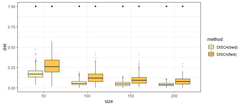
According to Table 1 and 2 of this counterexample, approximately 92% estimates from the backward elimination version of DISCA and 95% estimates from the forward selection version of DISCA have correct dimensions. From Fig. 1, when the sample size is greater than or equal to $100$, the average distance from the target subspace is less than or equal to $0.125$.

dim($\widehat{\mathcal{S}}_{x}$)	0	1	2	3
N=50	0	923	45	32
N=100	0	917	45	38
N=150	0	914	53	33
N=200	0	915	47	38

Table 1:          Frequencies of $\text{dim}(\mathcal{S}_{X})$.
(Forward-selection version of DISCA)

dim($\widehat{\mathcal{S}}_{x}$)	0	1	2	3
N=50	0	946	52	2
N=100	0	957	43	0
N=150	0	946	54	0
N=200	0	947	53	0

Table 2:          Frequencies of $\text{dim}(\mathcal{S}_{Y})$.
(Backward-elimination version of DISCA)

4.2 Comparison with Existing Methods

The following examples compare the performance of DISCA with existing simultaneous dimension reduction methods – CCA and DCS. In the simulation, the dimension of the target subspace is assumed to be known. Under this condition, the results are judged by the distance $dist(\cdot,\cdot)$ between the estimated subspaces $\widehat{\mathcal{S}}_{X}$, $\widehat{\mathcal{S}}_{Y}$ and the target subspaces $\mathcal{S}_{X}$ and $\mathcal{S}_{Y}$, which is the measure defined in Theorem 3.5.

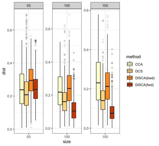
The counterexample in Section 4.1 is modified to compose Example 4.1, the Gaussian distribution example. In this case, the coordinates of $X$ are correlated, and the mutual relationship includes linear and polynomial nonlinear relationships. We add a new independent dimension to $Y$ to apply the DCS method. The comparison between the DISCA and DCS methods is shown in Fig. 2. Example 4.2 is a discrete distribution case with a symmetric, second-order polynomial relationship, with the comparison results summarized in Fig. 3. Example 4.3 is a heavy-tailed distribution case with a non-symmetric, nonpolynomial, and nonlinear mutual relationship, with the comparison results summarized in Fig. 4. We will consider three cases with varying sample sizes $N$, including $50$, $100$, and $150$. The In Example 4.2 and 4.3, the Condition 2.5 is not satisfied, and the target subspaces are set as central subspaces defined at the beginning of this section.

Example 4.1.

(Normal distribution example) Suppose $X\in\mathbb{R}^{3}$ and $Y\in\mathbb{R}^{3}$. We have

$$X=(X_{1},X_{2},X_{3})^{T},Y=(Y_{1},Y_{2},Y_{3})^{T}.$$

$X$ follows the multivariate normal distribution with zero mean and covariance matrix

$$\Sigma=\left(\begin{array}[]{ccc}1&0.5&0.5\\ 0.5&1&0.5\\ 0.5&0.5&1\end{array}\right).$$

$Y_{1}$ and $Y_{2}$ satisfies $Y_{1}=X_{1}+X_{2}+X_{3}+0.01\epsilon_{1},Y_{2}=(X_{1}+X_{2}+X_{3})^{2}+0.01\epsilon_{2},Y_{3}\sim N(0,1),$ where $\epsilon_{1},\epsilon_{2}$ are i.i.d. from the standard normal distribution.

The anticipated results would be

$$\mathcal{S}_{X}=span\left\{\left(\frac{1}{\sqrt{3}},\frac{1}{\sqrt{3}},\frac{1}{\sqrt{3}}\right)^{T}\right\};\quad\mathcal{S}_{Y}=span\left\{(1,0,0)^{T},(0,1,0)^{T}\right\}.$$

The boxplots of calculation results are in Fig. 2.

(a) $\log(dist(\widehat{\mathcal{S}}_{X},\mathcal{S}_{X})+1)$ by DISCA and DCS

(b) $\log(dist(\widehat{\mathcal{S}}_{Y},\mathcal{S}_{Y})+1)$ by DISCA and DCS

Figure 2: $\log(dist(\widehat{\mathcal{S}}_{X},\mathcal{S}_{X})+1)$ and $\log(dist(\widehat{\mathcal{S}}_{Y},\mathcal{S}_{Y})+1)$ of DISCA (back-elimination and forward-selection versions) and DCS in Example 1. The x-axis represents sample sizes $N=50,100,150$.

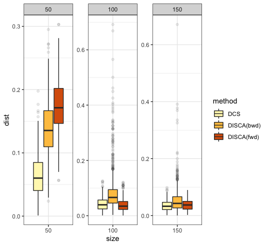
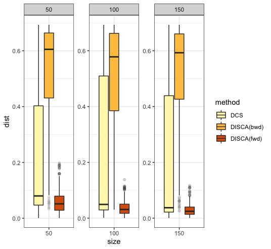
For estimates $\widehat{\mathcal{S}}_{X}$ of $\mathcal{S}_{X}$ in Example 4.1, the DCS method is better than two versions of the DISCA algorithm with sample size $N=50$. However, when the sample size is greater than $50$, the forward-selection version of DISCA is comparable with DCS. For estimates $\widehat{\mathcal{S}}_{Y}$ of $\mathcal{S}_{Y}$, outputs from the forward-selection version of DISCA are significantly better than that from DCS.

Example 4.2.

(Discrete distribution example) Suppose $X\in\mathbb{R}^{3}$ and $Y\in\mathbb{R}^{2}$. We have

$$X=(X_{1},X_{2},X_{3})^{T},Y=(Y_{1},Y_{2})^{T}.$$

$X_{i}\stackrel{{\scriptstyle\mbox{i.i.d.}}}{{\sim}}B(10,0.5),i=1,2,3;Y_{1}=\left(X_{1}+X_{2}+X_{3}\right)^{2}+0.01\epsilon,Y_{2}\sim B(10,0.35)$, where $\epsilon\sim N(0,1)$.

The anticipated results would be

$$\mathcal{S}_{X}=span\left\{\left(\frac{1}{\sqrt{3}},\frac{1}{\sqrt{3}},\frac{1}{\sqrt{3}}\right)^{T}\right\};\quad\mathcal{S}_{Y}=span\left\{(1,0)^{T}\right\}.$$

The boxplots of calculation results are in Fig. 3.

(a) $\log(dist(\widehat{\mathcal{S}}_{X},\mathcal{S}_{X})+1)$ by DISCA, DCS and CCA

(b) $\log(dist(\widehat{\mathcal{S}}_{Y},\mathcal{S}_{Y})+1)$ by DISCA, DCS and CCA

Figure 3: $\log(dist(\widehat{\mathcal{S}}_{X},\mathcal{S}_{X})+1)$ and $\log(dist(\widehat{\mathcal{S}}_{Y},\mathcal{S}_{Y})+1)$ of DISCA (back-elimination and forward-selection versions), DCS and CCA in Example 2. The x-axis represents sample sizes $N=50,100,150$.

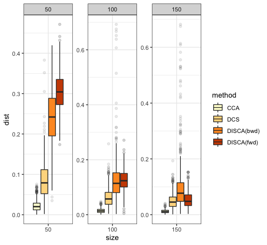
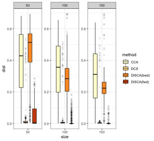
In this discrete example, the CCA method produces the smallest distance $dist(\widehat{\mathcal{S}}_{X},\mathcal{S}_{X})$. However, it is significantly weaker than DCS and DISCA in estimating $\mathcal{S}_{Y}$. When the sample size is $50$ or $100$, the DCS method outperforms the two versions of DISCA in estimating $\mathcal{S}_{X}$. It is comparable with the forward-selection version of DISCA in estimating $\mathcal{S}_{Y}$. When the sample size equals $150$, DCS is comparable with the forward-selection version of DISCA in estimating $\mathcal{S}_{X}$.

Example 4.3.

(Heavy-tailed distribution example) Suppose $X\in\mathbb{R}^{3}$ and $Y\in\mathbb{R}^{2}$. We have

$$X=(X_{1},X_{2},X_{3})^{T},Y=(Y_{1},Y_{2})^{T}.$$

$X_{i}\stackrel{{\scriptstyle\mbox{i.i.d.}}}{{\sim}}t(2),i=1,2,3;Y_{j}=\mbox{tanh}\left(X_{1}+X_{2}+X_{3}\right)+0.01\epsilon_{j},j=1,2$, where $\epsilon_{1},\epsilon_{2}\stackrel{{\scriptstyle i.i.d.}}{{\sim}}N(0,1)$.

The anticipated results would be

$$\mathcal{S}_{X}=span\left\{\left(\frac{1}{\sqrt{3}},\frac{1}{\sqrt{3}},\frac{1}{\sqrt{3}}\right)^{T}\right\};\quad\mathcal{S}_{Y}=span\left\{\left(\frac{1}{\sqrt{2}},\frac{1}{\sqrt{2}}\right)^{T}\right\}.$$

The boxplots of calculation results are in Fig. 4.

(a) $\log(dist(\widehat{\mathcal{S}}_{X},\mathcal{S}_{X})+1)$ by DISCA, DCS and CCA

(b) $\log(dist(\widehat{\mathcal{S}}_{Y},\mathcal{S}_{Y})+1)$ by DISCA, DCS and CCA

Figure 4: $\log(dist(\widehat{\mathcal{S}}_{X},\mathcal{S}_{X})+1)$ and $\log(dist(\widehat{\mathcal{S}}_{Y},\mathcal{S}_{Y})+1)$ of DISCA (back-elimination and forward-selection versions), DCS and CCA in Example 3. The x-axis represents sample sizes $N=50,100,150$.

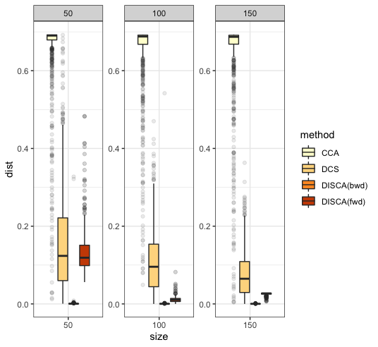
In this heavy-tailed distribution example, the estimated subspace $\widehat{\mathcal{S}}_{X}$ from CCA or the backward-elimination version of DISCA does not converge to the target subspace. The forward-selection version of DISCA produces estimates that converge to the target subspaces, outperforming DCS and CCA. For the estimation of $\mathcal{S}_{Y}$, the distances $dist(\widehat{\mathcal{S}}_{Y},\mathcal{S}_{Y})$ collected from two versions of DISCA are nearly zero, better than the other two methods.

From the above results, we can see that the CCA method is poor in the estimation process of $\mathcal{S}_{Y}$, revealing its incapability in detecting nonlinear relationship detection. The DCS method performs well in the discrete distribution example and can explore quadratic relationships. However, DCS’s performance is not good enough when the linear relationship is mixed with the second-order relationship or the random variable follows the heavy-tailed distribution. The backward-elimination version of DISCA cannot detect the second-order symmetric nonlinear relationship or perform satisfactorily in the heavy-tailed distribution case. However, when the nonlinear relationship is asymmetric, and the variable follows a non-heavy-tailed distribution, its performance is comparable or better. Finally, the estimates made by the forward-selection version of DISCA converge to the target subspaces in every case. When the sample size is small, it is sometimes weaker than DCS or the backward-elimination version of DISCA; as the sample size grows, its performance will be comparable or better.

Notice that the anticipated subspace differs from the target space defined in Definition 2.6 due to the violation of Condition 2.5. Despite this, the outputs from DISCA are still better than or comparable with those produced by CCA or DCS in the three simulation examples. The simulation results demonstrate that the DISCA algorithm, particularly the forward-selection version of DISCA, is more effective in situations involving nonlinear relationships or heavy-tailed distributions.

4.3 Higher Order Interactions

In some cases, the marginal dependency structure defined in Definition 2.4 and 2.6 is insufficient to describe mutual relationships. Compared with examples in Section 4.2, we construct an example with higher-order dependency where the independence sets $\mathcal{I}_{X}$ and $\mathcal{I}_{Y}$ do not compose linear subspaces. Moreover, the mutual relationship in this example forms a $V$-structure. The estimations from the forward-selection and backward-elimination versions of DISCA are compared to show their different properties in this case.

Suppose $X_{1},X_{2}\stackrel{{\scriptstyle i.i.d.}}{{\sim}}X$, $P(X=0)=P(X=1)=0.5$. $Y=I_{X_{1}+X_{2}\neq 1}$.

In this example, only a few estimated subspaces possess correct dimensions; therefore, rather than focusing on the distance between the output and the anticipated target result, we tabulate the estimated dimensions from the DISCA to display the results as in Table 3 and 4. For each sample size, we perform $200$ replicates.

Sample Size $N$	$dim(\widehat{\mathcal{S}}_{X})=0$	$dim(\widehat{\mathcal{S}}_{X})=1$	$dim(\widehat{\mathcal{S}}_{X})=2$
50	159	15	26
100	156	18	26
150	165	10	25
200	158	11	31

Table 3: $dim(\widehat{\mathcal{S}}_{X})$ – Backward-Elimination version of DISCA.

Sample Size $N$	$dim(\widehat{\mathcal{S}}_{X})=0$	$dim(\widehat{\mathcal{S}}_{X})=1$	$dim(\widehat{\mathcal{S}}_{X})=2$
50	3	0	197
100	1	0	199
150	2	1	197
200	2	1	197

Table 4: $dim(\widehat{\mathcal{S}}_{X})$ – Forward-Selection version of DISCA

From the collected observations in the table, we can observe that the backward-elimination version of DISCA tends to output a subspace with zero dimension. When the sample size increases from 50 to 200, the output $\widehat{\mathcal{S}}_{X}$ does not converge to a zero vector space. This could happen since the set of independent directions does not only contain $(1,0)$ and $(0,1)$.

For the forward-selection version DISCA, we could observe that the output would be the total space $\mathbb{R}^{2}$, implying that two dependent orthogonal directions can also be found.

So, suppose the DISCA algorithm is chosen as a preprocessing step to reduce the input dimension of data analysis. In that case, a forward-selection version of DISCA will likely include all necessary directions. On the contrary, the backward-elimination DISCA is more likely to guarantee that all directions in $\widehat{\mathcal{S}}_{X}$ and $\widehat{\mathcal{S}}_{Y}$ are dependent directions. Consequently, the output dimension of backward-elimination DISCA tends to be smaller than the anticipated result.

5 Conclusion

This paper focuses on the dimension reduction topic, which is beneficial for both computational efficiency and the accuracy of data analysis. The existing dimension reduction methods have imposed dimension and distribution assumptions on input variables, which leads to incapability in some circumstances. To loosen the assumptions of variable distributions in other dimension reduction techniques, including SDR-based methods, we first propose our target subspaces as $\mathcal{S}_{X}$ and $\mathcal{S}_{Y}$ which are different from central subspaces $\mathcal{S}_{X\mid Y}$ and $\mathcal{S}_{Y\mid X}$. With the reconstructed target subspaces, we provide an example where existing methods cannot tackle while the DISCA algorithm can output the correct result. Taking reformulated empirical distance covariance to estimate $\mathcal{S}_{X}$ and $\mathcal{S}_{Y}$, the DISCA algorithm calculates the dimension of subspace in sequential computing steps, rather than the bootstrap method in Iaci et al. [2016]. Furthermore, we provide theoretical non-asymptotic error bounds of the DISCA algorithm based on concentration inequalities of $U$-statistics to complement the implicit sample size requirement in the classical asymptotic convergence result and provide an explicit convergence rate. Both the Type i@ error and Type ii@ error are bounded by the non-asymptotic results, constraining the behavior of the DISCA algorithm in the worst case.

It is worth mentioning that for higher-order interactions, our method cannot produce accurate dimension reduction results. Extensions to the detection of $V$-structure dependency etc., are related to future research topics.

SUPPLEMENTARY MATERIAL

DISCA:

The DISCA zip file contains the appendices as well as the following items:

R-package for DISCA:

R-package DISCA contains code to perform the DISCA method described in the paper.

LA pollution-mortality data set:

A real dataset used to illustrate the DISCA method. (.txt file)

References

- Andrew et al. [2013] Galen Andrew, Raman Arora, Jeff Bilmes, and Karen Livescu. Deep canonical correlation analysis. In International Conference on Machine Learning, pages 1247–1255, 2013.
- Bach and Jordan [2002] Francis R Bach and Michael I Jordan. Kernel independent component analysis. Journal of machine learning research, 3(Jul):1–48, 2002.
- Chang et al. [2013] Billy Chang, Uwe Kruger, Rafal Kustra, and Junping Zhang. Canonical correlation analysis based on Hilbert-Schmidt independence criterion and centered kernel target alignment. In International Conference on Machine Learning, pages 316–324, 2013.
- Chen et al. [2019] Xianyan Chen, Qingcong Yuan, and Xiangrong Yin. Sufficient dimension reduction via distance covariance with multivariate responses. Journal of Nonparametric Statistics, 31(2):268–288, 2019.
- Cook [1998] R Dennis Cook. Principal hessian directions revisited. Journal of the American Statistical Association, 93(441):84–94, 1998.
- Cook and Ni [2005] R Dennis Cook and Liqiang Ni. Sufficient dimension reduction via inverse regression: A minimum discrepancy approach. Journal of the American Statistical Association, 100(470):410–428, 2005.
- Cook and Weisberg [1991] R Dennis Cook and Sanford Weisberg. Comment. Journal of the American Statistical Association, 86(414):328–332, 1991.
- Cook et al. [2023] R Dennis Cook, Liliana Forzani, and Lan Liu. Partial least squares for simultaneous reduction of response and predictor vectors in regression. Journal of Multivariate Analysis, 196:105163, 2023.
- Golub and Van Loan [2012] Gene H Golub and Charles F Van Loan. Matrix computations, volume 3. JHU Press, 2012.
- Huo and Székely [2016] Xiaoming Huo and Gábor J Székely. Fast computing for distance covariance. Technometrics, 58(4):435–447, 2016.
- Iaci et al. [2016] Ross Iaci, Xiangrong Yin, and Lixing Zhu. The dual central subspaces in dimension reduction. Journal of Multivariate Analysis, 145:178–189, 2016.
- Lai and Fyfe [1999] Pei Ling Lai and Colin Fyfe. A neural implementation of canonical correlation analysis. Neural Networks, 12(10):1391–1397, 1999.
- Lai and Fyfe [2000] Pei Ling Lai and Colin Fyfe. Kernel and nonlinear canonical correlation analysis. International Journal of Neural Systems, 10(05):365–377, 2000.
- Li [1991] Ker-Chau Li. Sliced inverse regression for dimension reduction. Journal of the American Statistical Association, 86(414):316–327, 1991.
- Li [1992] Ker-Chau Li. On principal hessian directions for data visualization and dimension reduction: Another application of stein’s lemma. Journal of the American Statistical Association, 87(420):1025–1039, 1992.
- Maurer and Pontil [2019] Andreas Maurer and Massimiliano Pontil. Uniform concentration and symmetrization for weak interactions. In Conference on Learning Theory, pages 2372–2387. PMLR, 2019.
- Sheng and Yin [2013] Wenhui Sheng and Xiangrong Yin. Direction estimation in single-index models via distance covariance. Journal of Multivariate Analysis, 122:148–161, 2013.
- Sheng and Yin [2016] Wenhui Sheng and Xiangrong Yin. Sufficient dimension reduction via distance covariance. Journal of Computational and Graphical Statistics, 25(1):91–104, 2016.
- Székely and Rizzo [2014] Gábor J Székely and Maria L Rizzo. Partial distance correlation with methods for dissimilarities. The Annals of Statistics, 42(6):2382–2412, 2014.
- Székely et al. [2007] Gábor J Székely, Maria L Rizzo, Nail K Bakirov, et al. Measuring and testing dependence by correlation of distances. The annals of statistics, 35(6):2769–2794, 2007.
- Székely et al. [2009] Gábor J Székely, Maria L Rizzo, et al. Brownian distance covariance. The Annals of Applied Statistics, 3(4):1236–1265, 2009.
- Wang and Xia [2008] Hansheng Wang and Yingcun Xia. Sliced regression for dimension reduction. Journal of the American Statistical Association, 103(482):811–821, 2008.
- Xia et al. [2002] Yingcun Xia, Howell Tong, Wai Keung Li, and Li-Xing Zhu. An adaptive estimation of dimension reduction space. Journal of the Royal Statistical Society: Series B (Statistical Methodology), 64(3):363–410, 2002.
- Yin [2004] Xiangrong Yin. Canonical correlation analysis based on information theory. Journal of multivariate analysis, 91(2):161–176, 2004.
- Yin et al. [2008] Xiangrong Yin, Bing Li, and R Dennis Cook. Successive direction extraction for estimating the central subspace in a multiple-index regression. Journal of Multivariate Analysis, 99(8):1733–1757, 2008.
- Zhu and Zeng [2006] Yu Zhu and Peng Zeng. Fourier methods for estimating the central subspace and the central mean subspace in regression. Journal of the American Statistical Association, 101(476):1638–1651, 2006.