Evident black hole-bulge coevolution in the distant universe
Abstract
Observations in the local universe show a tight correlation between the masses of supermassive black holes (SMBHs; ) and host-galaxy bulges (), suggesting a strong connection between SMBH and bulge growth. However, direct evidence for such a connection in the distant universe remains elusive. We have studied sample-averaged SMBH accretion rate () for bulge-dominated galaxies at . While previous observations found is strongly related to host-galaxy stellar mass () for the overall galaxy population, our analyses show that, for the bulge-dominated population, is mainly related to SFR rather than . This -SFR relation is highly significant, e.g. (Pearson statistic) at . Such a -SFR connection does not exist among our comparison sample of galaxies that are not bulge-dominated, for which appears to be the main determinant of SMBH accretion. This difference between the bulge-dominated and comparison samples indicates that SMBHs only coevolve with bulges rather than the entire galaxies, explaining the tightness of the local - correlation. Our best-fit -SFR relation for the bulge-dominated sample is (solar units). The best-fit ratio () for bulge-dominated galaxies is similar to the observed values in the local universe. Our results reveal that SMBH and bulge growth are in lockstep, and thus non-causal scenarios of merger averaging are unlikely the origin of the - correlation. This lockstep growth also predicts that the - relation should not have strong redshift dependence.
keywords:
galaxies: evolution – galaxies: active – galaxies: nuclei – quasars: supermassive black holes – X-rays: galaxies1 Introduction
One of the essential challenges of extragalactic astronomy is to understand the connection between supermassive black holes (SMBHs) and their host galaxies. It is well established that the masses of SMBHs () are tightly correlated with the stellar masses of host-galaxy classical bulges () in the local universe (the Magorrian relation; e.g. Magorrian et al. 1998; Ferrarese & Merritt 2000; Gebhardt et al. 2000; Häring & Rix 2004; Kormendy & Ho 2013). The intrinsic scatter of the - correlation is only dex (Kormendy & Ho, 2013). This tight correlation is surprising considering that is only a tiny fraction (a few thousandths) of . Therefore, some fundamental connections between the growth of SMBHs and host-galaxy bulges likely exist over cosmic history. These physical connections are often termed as “SMBH-bulge coevolution”.
Tremendous observational efforts have been made to identify these mysterious connections. It has been found that the cosmic evolution of SMBH accretion rate (BHAR) density and star formation rate (SFR) density are broadly similar, both peaking at (e.g. Aird et al., 2010, 2015; Mullaney et al., 2012; Madau & Dickinson, 2014; Ueda et al., 2014). However, from observations of active galactic nuclei (AGNs), the SFR is a relatively flat function of the observed BHAR at a given redshift (e.g. Harrison et al., 2012; Rosario et al., 2013; Azadi et al., 2015; Stanley et al., 2015; Lanzuisi et al., 2017; Stanley et al., 2017; Dai et al., 2018). This apparent lack of a strong SFR-BHAR connection might be caused by AGN variability. While star formation activity is stable on time scales longer than Myr, SMBH accretion could vary strongly on much shorter time scales ( yr; e.g. Martini 2004; Kelly et al. 2010; Novak et al. 2011; Sartori et al. 2018). An intrinsic connection between SFR and long-term average BHAR might be hidden by this strong AGN variability.
To obtain long-term average BHAR, the ideal way is to observe a galaxy for at least millions of years, which is presently infeasible. Practically, it has been proposed to adopt sample-averaged BHAR () as a proxy of long-term average BHAR (e.g. Chen et al., 2013; Hickox et al., 2014). Indeed, a positive -SFR connection has been observed (e.g. Chen et al., 2013; Hickox et al., 2014; Lanzuisi et al., 2017; Yang et al., 2017). However, Yang et al. (2017) show, via partial correlation analyses (PCOR), that is actually more strongly related to host-galaxy total stellar mass () than SFR (also see Fornasini et al. 2018 for a similar conclusion). Their results suggest that the apparent -SFR relation is only a secondary effect resulting from a primary - relation and the star-formation main sequence. Yang et al. (2018b) further show that once is carefully controlled, SMBH accretion is largely independent of the cosmic environment of the host galaxies, consistent with previous AGN clustering studies (e.g. Georgakakis et al. 2014; Leauthaud et al. 2015; Mendez et al. 2016; Powell et al. 2018). Motivated by the important role of in connecting SMBHs and host galaxies, Yang et al. (2018a) quantitatively derived the - relation at different redshifts up to . Aided by the stellar-mass history from Behroozi et al. (2013), Yang et al. (2018a) predicted the typical - relation in the local universe. At the massive end ( ) of their - relation, their ratio is , similar to observed values (e.g. Häring & Rix 2004; Kormendy & Ho 2013). This agreement is expected, as the bulge becomes dominant and for massive galaxies.
Despite the - relation being generally supported by observations, it cannot straightforwardly explain the tightness of the - correlation. The key to the origin of the tight - correlation might be related to the morphology of host galaxies, since is only correlated with the masses of classical bulges rather than other galactic components such as pseudo-bulges or disks (e.g. Kormendy & Ho 2013 and references therein). Therefore, SMBH growth might be related to star formation activity of the bulge only. To investigate this potential SMBH-bulge coevolution, one should ideally study the relation between and bulge SFR in the distant universe. However, with current facilities, it is infeasible to separate the bulge SFR from total SFR when disks are present. In this work, we focus on a sample of bulge-dominated galaxies for which bulge SFR total SFR. If SMBHs indeed coevolve with host-galaxy bulges, we expect a strong correlation between and SFR for these bulge-dominated galaxies over cosmic history.
Our bulge-dominated sample is selected from the Cosmic Assembly Near-Infrared Deep Extragalactic Legacy Survey (CANDELS) where deep HST -band observations are available (Grogin et al. 2011; Koekemoer et al. 2011). X-ray emission is a robust tracer of SMBH accretion (e.g. Brandt & Alexander 2015 and references therein). The CANDELS fields also have deep Chandra X-ray observations, allowing us to estimate reliable for any given sample of galaxies (e.g. Yang et al. 2017, 2018b).
This paper is structured as follows. In §2, we describe the data used in this work and define our samples. In §3, we perform data analyses and present the results. We discuss our results in §4. We summarize our work and discuss future prospects in §5.
Throughout this paper, we assume a cosmology with km s-1 Mpc-1, , and . We adopt a Chabrier initial mass function (IMF; Chabrier 2003). Quoted uncertainties are at the (68%) confidence level. We express , , and in units of , SFR and in units of yr-1. indicates AGN X-ray luminosity at rest-frame 2–10 keV and is in units of erg s-1.
2 Data and Sample
Our analyses are based on the five CANDELS fields, i.e., GOODS-S, GOODS-N, EGS, UDS, and COSMOS (Grogin et al., 2011; Koekemoer et al., 2011). All these fields have multiwavelength observations from HST, Spitzer, and ground-based telescopes such as Subaru and VLT. These high-quality data sets allow for measurements of galaxy morphology (§2.1), stellar mass (; §2.2), and star-formation rate (SFR; §2.2). FIR observations from Herschel are also available in these fields, enabling robust SFR estimation based on cold-dust emission (§2.2). All of the five CANDELS fields have Chandra X-ray observations from which we derive (§2.4). We define our sample in §2.3 and the sample properties are summarized in Tab. 1.
| Field | Area | Gal. # | Spec./Photo. # | Galaxy Ref. | B.-D. (X) | Comp. (X) | X. Dep. | X-ray Ref. |
|---|---|---|---|---|---|---|---|---|
| (1) | (2) | (3) | (4) | (5) | (6) | (7) | (8) | (9) |
| GOODS-S | 170 | 1,504 | 727/777 | Santini et al. (2015) | 398 (100) | 1,106 (241) | 7 Ms | Luo et al. (2017) |
| GOODS-N | 170 | 1,855 | 391/1,464 | Barro et al., in prep. | 483 (71) | 1,372 (168) | 2 Ms | Xue et al. (2016) |
| EGS | 200 | 2,446 | 219/2,227 | Stefanon et al. (2017) | 591 (48) | 1,855 (105) | 800 ks | Nandra et al. (2015) |
| UDS | 200 | 2,128 | 254/1,874 | Santini et al. (2015) | 549 (42) | 1,579 (75) | 600 ks | Kocevski et al. (2018) |
| COSMOS | 220 | 2,369 | 10∗/2,359 | Nayyeri et al. (2017) | 603 (22) | 1,766 (39) | 160 ks | Civano et al. (2016) |
| Total | 960 | 10,302 | 1,601/8,701 | – | 2,624 (283) | 7,678 (628) | – | – |
Note. — (1) CANDELS field name. (2) Field area in arcmin2. (3) Number of galaxies in our -complete sample (§2.3). (4) Number of spec-/photo- sources (§2.2). (5) Reference for CANDELS galaxy catalog. (6) & (7) Sample size of bulge-dominated and comparison galaxies (§2.3). The number in parentheses means the sample size of X-ray detected sources. (8) X-ray depth in terms of exposure time (§2.4). (9) Reference for X-ray catalog.
Although there are more than 500 spec- available in the CANDELS region of COSMOS, the latest version of the CANDELS/COSMOS catalog is mostly based on photo-. Future releases of the CANDELS/COSMOS catalog will adopt spec- when available (H. Nayyeri 2018, private communication).
2.1 Morphology
Rest-frame optical/NIR light is essential for morphological measurements (e.g. Conselice, 2014). The HST band, centered at m, can cover rest-frame optical/NIR wavelengths up to . We adopt the -band morphological measurements in Huertas-Company et al. (2015a) that are based on machine learning for CANDELS galaxies with . The machine-learning technique is chosen to approximate visual morphologies from humans, and is trained with a galaxy sample that has morphological measurements performed by human classifiers (Kartaltepe et al., 2015). This training sample has the same magnitude cut () as reliable visual morphological measurements are difficult at fainter magnitudes. For each galaxy, the Huertas-Company et al. (2015a) catalog provides five fractional numbers, i.e., , , , , and . These fractions represent the probabilities that a hypothetical classifier would have voted for a galaxy having a spheroid, a disk, and some irregularities, being point-like and unclassifiable, respectively. Note that the sum of the fractions might exceed unity, because, for example, a galaxy might have both spheroidal and disky features simultaneously.
A high value indicates that the source might be a spurious detection, e.g. the spikes of a bright star being falsely detected as a source (see, e.g. Fig. 13 of Huertas-Company et al. 2015a). Sources with high value might be stars or broad-line (BL) AGNs. Due to strong light from the AGN central engine, morphology measurements of host galaxies are unreliable for luminous BL AGNs (e.g. §5.3 of Brandt & Alexander 2015). We exclude the of sources that have or greater than any of , , and . Upon visual inspection, the excluded sources are indeed spurious detections or point-like. Morphological measurements are challenging at high redshift and our work probes up to . We discuss some possible redshift-related effects on our results in §3.4.
2.2 Redshift, Stellar Mass, and Star Formation Rate
We obtain redshift measurements from the CANDELS catalogs (see Tab. 1). These measurements are spectroscopic redshifts (spec-) or photometric redshifts (photo-). The photo- measurements are based on dedicated photometry extracted with careful consideration of PSF sizes and source shapes (e.g. Guo et al. 2013; Galametz et al. 2013). Compared to the available spec-, the photo- shows high quality, with and an outlier fraction of 2%.111Here, is defined as , and outliers are defined as sources having . As in §2.1, we discard the 79 spectroscopic BL AGNs reported in the literature (Barger et al. 2003; Silverman et al. 2010; Cooper et al. 2012; Newman et al. 2013; Marchesi et al. 2016; Suh et al., in prep.).
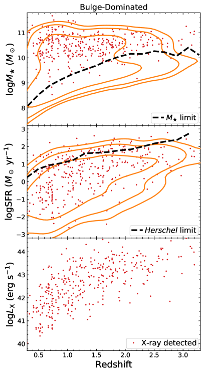
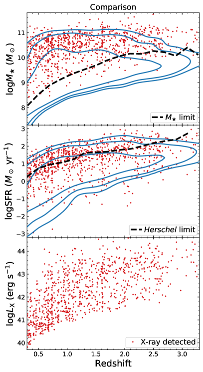
The CANDELS catalogs also provide stellar mass () and star formation rate (SFR) measurements from independent teams. Following Yang et al. (2017), we adopt the median and SFR values from the five available teams (2aτ, 6aτ, 11, 13aτ, and 14a).222For GOODS-N, only three teams are available (2aτ, 6aτ, and 14a) for now. Fig. 1 (top) shows as a function of redshift for galaxies that have morphological measurements (§2.1). We limit our analyses to a -complete (corresponding to ) sample (§2.3). The limiting () for is also displayed in Fig. 1. The -redshift curve is derived based on an empirical method (e.g. Ilbert et al. 2013). We first divide our sources into narrow redshift bins with width of . For each redshift bin, we calculate for individual galaxies in the bin. We then adopt as the 90th percentile of the distribution for the redshift bin.
The CANDELS and SFR are based on SED fitting of rest-frame UV-to-NIR photometry using galaxy templates. As demonstrated by previous works (e.g. Luo et al., 2010; Yang et al., 2017; Kocevski et al., 2018), the rest-frame UV-to-NIR light is often predominantly contributed by galaxy component rather than the AGN component for X-ray AGNs in the CANDELS fields. Also, we have removed BL AGNs that might have strong AGN components in their UV-to-NIR SED. Therefore, the AGN SED contribution should not qualitatively affect our results (see §3.4 for other evidence).
The SED-based SFR estimation, which is physically based on obscuration-corrected UV light, is reliable for low-to-moderate levels () of star-formation activity. However, it tends to underestimate SFR in the high-SFR regime, possibly due to strong dust obscuration (e.g. Wuyts et al., 2011; Whitaker et al., 2017; Yang et al., 2017). To alleviate this issue, we adopt SFR from FIR photometry of Herschel when available (Lutz et al. 2011; Oliver et al. 2012; Magnelli et al. 2013). The photometry has been extracted using Spitzer/MIPS 24 m priors and source-blending issues have been carefully addressed. The FIR-based SFR is more robust than the SED-based SFR, especially in the high-SFR regime (e.g. Chen et al., 2013; Yang et al., 2017). Due to limited sensitivity, Herschel can only detect sources with the highest SFR at a given redshift. There are five Herschel bands available for the CANDELS fields, i.e., 100 m, 160 m, 250 m, 350 m, and 500 m. We only utilize robust detections with . We discard the 100 m band at redshifts above , because the observed 100 m corresponds to rest-frame m which might be contaminated by hot-dust emission powered by AGN activity. We adopt the reddest available Herschel band to estimate SFR, since longer wavelengths are “freer” from possible AGN emission. We calculate SFR from FIR flux following the procedure in Chen et al. (2013) and Yang et al. (2017). We first derive galaxy total IR luminosity () from FIR flux based on the star-forming galaxy templates of Kirkpatrick et al. (2012). We adopt the and templates for and sources, respectively. We then obtain SFR as
| (1) |
Fig. 1 (middle) shows SFR (based on SED or FIR) as a function of redshift for all galaxies.
The comparison sample has a higher fraction of FIR-based SFR measurements than the bulge-dominated sample (32% vs. 9%), because the former generally has stronger star-formation activity than the latter. To investigate whether this difference in SFR measurements could bias our results, we have tested cutting our () sample at yr-1 ( yr-1), below which the SFR measurements are mostly SED-based (see Fig. 1). Under these cuts, our results do not change qualitatively.333We cannot perform a similar test for high-SFR galaxies with Herschel detections, because the sample size of Herschel-detected sources is too small. We have also tested our results using SED-based SFR only for the entire galaxy sample and our conclusions still hold. It is well known that SFR measurements from SEDs and the FIR do not always agree (e.g. Buat et al., 2010; Rodighiero et al., 2014), and Yang et al. (2017) found that the statistical scatter between these two methods is dex. This level of scatter is unlikely to be seriously problematic to our statistical analyses (§3.2), since our SFR bin sizes are typically dex. To verify this point, we perturb our SFR measurements by 0–0.5 dex randomly and our results below in §3 do not change qualitatively after the perturbation. Yang et al. (2017) found the systematic offset between SED-based and FIR-based SFRs is typically small for the general galaxy population ( dex), and this level of systematic should not change our main conclusions considering our relatively large SFR bin sizes. However, Symeonidis et al. (2016) considered that, for strong AGNs, FIR-based SFR might be systematically overestimated due to the contamination of AGN-heated dust. To assess this potential issue, we test our results by using SED-based SFR only for strong AGNs (), and our results below do not change qualitatively. Therefore, our main conclusions should be robust against uncertainties of SFR measurements.
2.3 The Bulge-Dominated and Comparison Samples
Our analyses are based on a bulge-dominated sample and a comparison sample. In this Section, we detail the selections of these two samples. We first select all galaxies for which morphology measurements are available (§2.1). As in §2.1 and §2.2, we exclude BL AGNs, stars, and false detections. We then divide these galaxies into two redshift bins, i.e., and for our analyses. The relatively broad redshift bins are necessary to guarantee sufficiently large samples for our statistical analyses (§3). We have also tested on narrower redshift bins and found our qualitative results do not change, although the statistical scatter becomes larger due to reduced sample sizes. Therefore, the two wide redshift bins ( and ) should not bias our results, and we adopt them throughout this paper.
We select -complete samples for the two redshift bins. The limiting at and are and , respectively (see Fig. 1). Therefore, we limit our analyses to and galaxies for the low and high redshift bins, respectively. These thresholds are below the characteristic of the stellar-mass function (SMF), i.e., at (e.g. Tomczak et al., 2014; Davidzon et al., 2017). The stellar-mass density above these cuts is and of the total for the low and high redshift bins, respectively (calculated with the SMF in Behroozi et al. 2013). After applying the cuts, our sample does not include dwarf galaxies (). Aside from technical constraints, the exclusion of dwarf galaxies is also motivated by our major science goal, i.e. investigating the origin of the - relation. Since the - relation is mostly established for (e.g. Kormendy & Ho, 2013), we should also focus on relatively massive galaxies rather than dwarf galaxies.
The basic properties of the -complete sample are summarized in Tab. 1. In the -complete sample, we classify a source as bulge-dominated if it satisfies , , and . These empirical criteria are suggested by several previous studies (e.g. Huertas-Company et al. 2015b, 2016; Kartaltepe et al. 2015). As indicated by these criteria, the term “bulge-dominated” refers to galaxies that only display a significant spheroidal component, without obvious disky and/or irregular components. We note that different authors may adopt different terminology for the bulge-dominated galaxies (e.g. “spheroid-like”; e.g. Conselice 2014). If a galaxy does not meet these criteria, we include it in our comparison sample, i.e., galaxies that are not bulge-dominated. The bulge-dominated and comparison samples have 2,600 and 7,700 galaxies, respectively (see Tab. 1). Our analyses in §3 are based on these two samples.
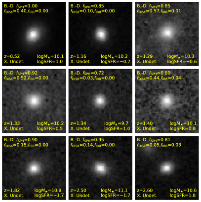
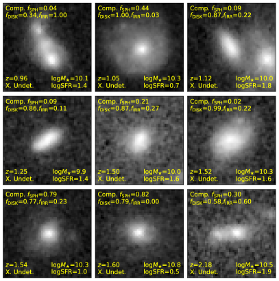
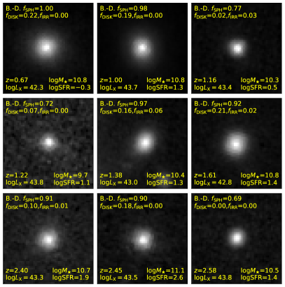
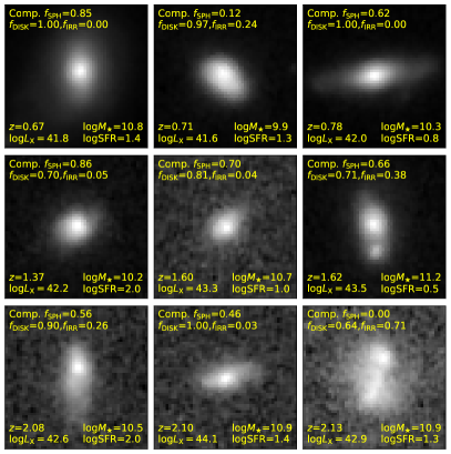
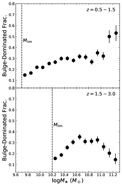
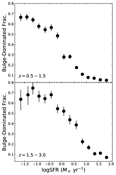
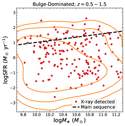
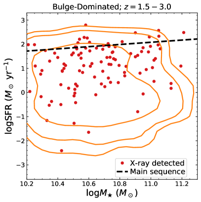
In Fig. 2, we show some random -band cutouts for the bulge-dominated and comparison samples, respectively. The fractions of bulge-dominated galaxies are both for the low and high redshift bins. Fig. 3 shows the fraction of bulge-dominated galaxies as a function of and SFR, respectively. At the high- end (), the bulge-dominated fraction in the low-redshift bin is much higher than that in the high-redshift bin ( vs. ). This is probably due to the fact that galaxy mergers/interactions for massive galaxies are increasingly prevalent toward high redshift, and thus galaxy irregularities are much stronger toward the early universe (e.g. Conselice, 2014; Marsan et al., 2018). The bulge-dominated fraction drops significantly toward high SFR, indicating that bulge-dominated galaxies tend to have low SFR. Similar trends have also been found in previous studies (e.g. Huertas-Company et al. 2015b, 2016). The underlying physical reason might be “morphological quenching”, such that bulges can effectively suppress star formation (e.g. Martig et al., 2009).
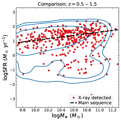
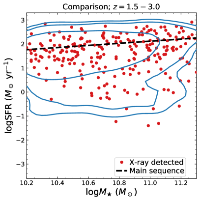
Fig. 4 displays the source distributions on the SFR- plane for the bulge-dominated and comparison samples, respectively. The bulge-dominated sample tends to lie below the star-formation main sequence, while the majority of the comparison sample appears to be on the main sequence. However, we note that our morphological classification is essentially different from a star-forming vs. quiescent classification. For example, the quiescent population in our sample is made up of bulge-dominated galaxies and comparison galaxies. While the main population of the comparison sample lies on the main sequence, there is a non-negligible fraction () of comparison galaxies lying significantly ( dex) below the main sequence. We have visually checked the HST cutouts of these low-SFR sources, and found they appear to have significant disk/irregular components. Therefore, the existence of such a low-SFR population among our comparison sample is likely intrinsic, and does not appear to be caused by morphological misclassification.
2.4 Black Hole Accretion Rate
All five CANDELS fields have deep X-ray observations from Chandra. Tab. 1 lists the X-ray depth and number of X-ray detected sources for each CANDELS field. We calculate contributed by both X-ray detected and undetected sources, and thus the resulting should cover essentially all SMBH accretion. This procedure allows us to seamlessly analyze all sources in different CANDELS fields which have different X-ray depths. We have also repeated our analyses but without sources in COSMOS, which has X-ray depth much shallower than other fields (see Tab. 1), and our results do not change qualitatively. For each X-ray detected source, we calculate from the X-ray flux from the corresponding X-ray catalog assuming a photon index of (e.g. Yang et al. 2016; Liu et al. 2017). Following Yang et al. (2018b), we choose, in order of priority, hard-band (observed-frame keV), full-band (observed-frame keV), or soft-band (observed-frame keV) flux to minimize X-ray obscuration effects. Indeed, Yang et al. (2018b) estimated that, under this scheme of band choice, the X-ray flux decrease due to obscuration is typically small () for bright sources in CDF-S, for which there are enough photons to assess obscuration. We increase the X-ray fluxes of our X-ray sources by 20% to account for the average systematic effect from obscuration.
For X-ray undetected sources, we employ a stacking technique to include their X-ray emission. We perform this process on full-band X-ray images.444For the EGS field, we use the X-ray image from Goulding et al. (2012), since Nandra et al. (2015) did not produce the X-ray image for the entire EGS field. We generally follow the steps in Vito et al. (2016), and we briefly summarize this procedure below. First, we mask X-ray detected sources in the X-ray images. We choose masking radii () of , , and for sources with net counts , , and , respectively. Here, means the radius for a 90% encircled-energy fraction (EEF), and it is a function of off-axis angle (see Appendix A of Vito et al. 2016). After source masking, we derive the net count rate for X-ray undetected sources. To enhance signal-to-noise, we adopt an aperture radius , , , and for sources with off-axis angle , , , and , respectively. We discard sources whose off-axis angle is and/or whose apertures overlap with masked regions. The counts in the apertures include contributions from both sources and background, and we need to subtract the background counts. We estimate the background counts in an annulus with inner and outer radii of and , respectively. Due to the limited aperture size, the net counts encircled in the aperture only represent a fraction of the total net counts. We perform an aperture correction for each source, depending on the aperture size adopted. For example, if for a source, we divide the aperture net counts by 80% to recover the total net counts. We then obtain the count rate by dividing the total net counts by the exposure time at the position of the source. For sources in each field, we derive fluxes by multiplying the count rates by a constant factor, which is the median flux/count-rate ratio of X-ray detected sources in the field. Finally, for a group of X-ray undetected sources, we can obtain their average X-ray luminosity () from the average X-ray flux and redshift, assuming . Our derived SMBH accretion power is mostly contributed by the X-ray detected sources, and the stacking procedure typically accounts for less than 20% of the accretion power.
For X-ray detected objects, we have for individual sources; for X-ray undetected sources, we have for any group of sources. We can then calculate average AGN bolometric luminosity for any sample of sources as
| (2) |
Here, and are the numbers of X-ray detected and undetected sources in the sample. is the expected luminosity from X-ray binaries (XRBs) and is the average XRB luminosity for the stacked sources. To obtain and , we adopt model 269 of Fragos et al. (2013) which describes XRB X-ray luminosity as a linear function of and SFR. Model 269 is a theoretical model favored by the observations of galaxies at (Lehmer et al., 2016). The expected X-ray emission from XRBs only accounts for of the total X-ray power, and thus the uncertainties related to the XRB modelling should not affect our analyses significantly. and are the -dependent bolometric corrections at and , respectively. We adopt the bolometric-correction model from Hopkins et al. (2007).555As pointed out in Footnote 4 of Merloni & Heinz (2013), the in Hopkins et al. (2007) appears to be overestimated due to the double counting of IR reprocessed emission. Following Merloni & Heinz (2013), we multiply the in Hopkins et al. (2007) by a factor of 0.7 to address this issue. Assuming a constant radiative efficiency of , we can convert to as
| (3) |
where is the speed of light. The adopted is motivated by observations (see, e.g. §3.4 of Brandt & Alexander 2015). We obtain the uncertainties with a bootstrapping technique (e.g. §2.3 of Yang et al. 2017).
As explained in §1, the quantity is designed to approximate long-term average SMBH accretion rate, and has been widely adopted in the studies of AGN-galaxy relations (e.g. Chen et al. 2013; Hickox et al. 2014; Yang et al. 2017, 2018a, 2018b; Fornasini et al. 2018). Some works proposed to recover the full distribution of BHAR as a function of galaxy properties (e.g. Volonteri et al. 2015; Georgakakis et al. 2017; Aird et al. 2018b, a), and quantities such as and duty cycle can then be derived. However, detailed modelling of the BHAR distribution at given , SFR, and morphological type is beyond the scope of this work, and we leave it to future studies.
3 Analyses and Results
In this Section, we study as a function of SFR and (§3.1). We address the question of whether is mainly related to SFR or in §3.2. All these analyses are performed for the bulge-dominated and comparison samples, respectively. In Appendix A, we perform the same analyses for all galaxies. In §3.3, we quantify the -SFR relation for the bulge-dominated sample.
3.1 BHAR as a Function of SFR and
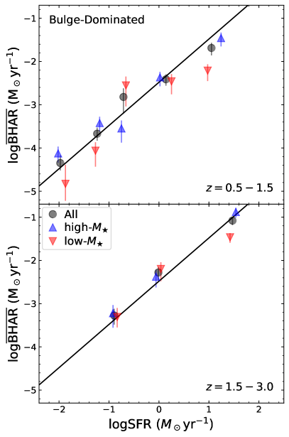
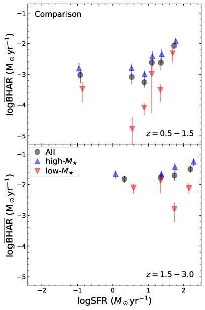
We plot the as a function of SFR for our bulge-dominated and comparison samples, respectively, in Fig. 5 (black points). In each panel, the bins are chosen to include approximately the same number of sources, and this approach is to reach similar signal-to-noise (S/N) ratios for the bins. Adjusting the bins does not change our conclusions qualitatively, although the statistical scatter of measurements increases.
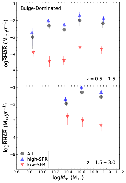
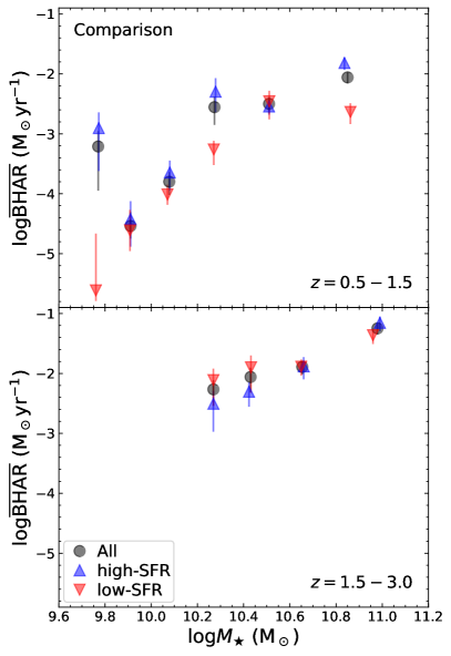
For the bulge-dominated sample, rises strongly from low to high SFR by a factor of () and (). In contrast, for the comparison sample, only increases by a factor of () and () from low to high SFR. We show vs. in Fig. 6 (black points). For the bulge-dominated sample, there is no strong correlation between and . For the comparison sample, appears to rise toward high in general. We note that, due to our limited sample size, statistical fluctuations can be strong sometimes. For example, for the black point at in Fig. 6 (right), the is mostly contributed by a single source. These fluctuations inevitably cause some scatter in Figs. 5 and 6.
3.2 Is Mainly Related to SFR or ?
In this Section, we address the question of whether is mainly related to SFR or for the bulge-dominated and comparison samples, respectively. The analysis methods here are similar to those in Yang et al. (2017). We compare our results with Yang et al. (2017) in Appendix A.
In Fig. 5, we divide each SFR bin into two bins with above and below the median of the SFR bin, respectively. In general, the high- and low- bins have similar for the bulge-dominated sample. However, the high- bins have significantly higher than the corresponding low- bins for the comparison sample. Similarly, in Fig. 6, we also divide each bin into high-SFR and low-SFR bins. The high-SFR bins have much higher than the corresponding low-SFR bins for the bulge-dominated sample. In contrast, the high-SFR and low-SFR bins have similar for the comparison sample.
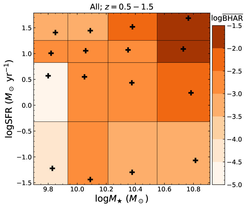
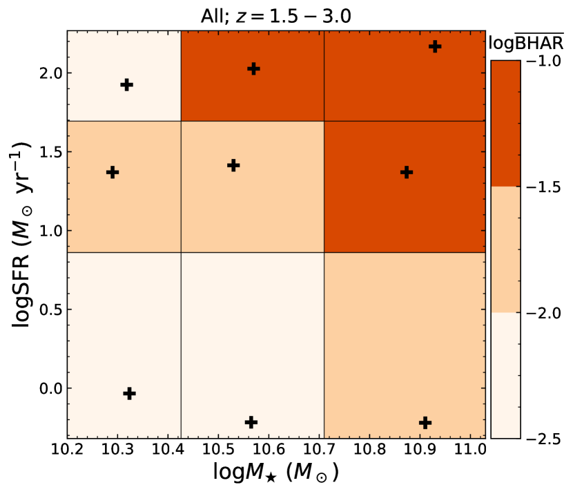
The results above qualitatively indicate that might primarily depend on SFR rather than for the bulge-dominated sample and that the situation is the opposite for the comparison sample. To further test this point, we perform partial-correlation (PCOR) analyses with pcor.r in the r statistical package (Kim, 2015). We first bin sources based on both SFR and and calculate for each bin, and Fig. 7 shows the results. Following Fig. 5, the bins for the -axis (-axis) include similar numbers of sources. Adjusting the bins does not affect our results qualitatively. We input the median , median , and in each bin to pcor.r and calculate the significance levels for the - and -SFR relations, respectively. The PCOR tests are performed with the Pearson and Spearman statistics, respectively, and the results are summarized in Tab. 2. These results show that, for the bulge-dominated sample, the -SFR correlation is significant () while the - correlation is not (). For the comparison sample, the - correlation is significant while the -SFR correlation is not. These conclusions are also supported by Figs. 5 and 6. We note that the lack of a significant -SFR relation for the comparison sample is unlikely to be caused by X-ray obscuration effects, because the effects of obscuration on our measurements are generally small (see §2.4).
Fig. 5 (left) is the key plot in this paper. It displays the strong -SFR connection and qualitatively demonstrates that the -SFR relation cannot be significantly split by . We have also tested dividing each SFR bin by other galaxy properties (instead of ) such as (§2.1) and rest-frame color, and none of these parameters can significantly split the -SFR relation. Therefore, the strong -SFR correlation is likely fundamental.
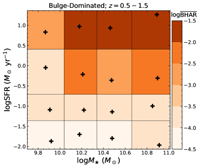
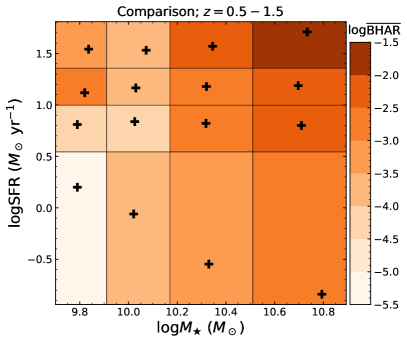
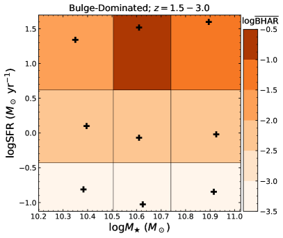
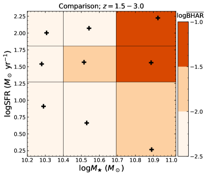
| Bulge-Dominated; | ||
|---|---|---|
| Relation | Pearson | Spearman |
| - | () | () |
| - | () | () |
| Bulge-Dominated; | ||
| Relation | Pearson | Spearman |
| - | () | () |
| - | () | () |
| Comparison; | ||
| Relation | Pearson | Spearman |
| - | () | () |
| - | () | () |
| Comparison; | ||
| Relation | Pearson | Spearman |
| - | () | () |
| - | () | () |
3.3 Quantification of the -SFR Relation
In §3.2, we find that is mainly correlated with SFR rather than for the bulge-dominated sample. To quantify this -SFR relation, we fit the data points in Fig. 5 (left; black points) with a log-linear model. For convenience, we list the sample properties of each data point in Tab. 3. We adopt a standard least- fitting method implemented by a python package scipy.optimize.curve_fit. We first fit the data points in the two redshift bins independently, and the results are
| (4) |
Considering the best-fit parameters are similar for the two redshift bins, we fit all the data points in both redshift bins simultaneously. The best-fit model is
| (5) |
where the errors are calculated under a 68% confidence level. The reduced of the fit is 0.8 (), showing that the fit quality is acceptable. Considering that the slope of the best-fit model is close to unity, we also fit the data with slope fixed to unity. This procedure results in
| (6) |
The fit quality is also acceptable, with reduced of 1.2 (). This best-fit model is displayed in Fig. 5 (left). The best-fit /SFR ratio in this model is .
Our does not include the accretion from BL AGNs (§2). Here, we consider this missed accretion power statistically. We first construct a non-BL AGN sample with and redshift matched with the spectroscopic BL AGN sample (§2.2): for each BL AGN, we randomly select a “nearby” non-BL AGN in the - plane (within and ). We find that of these non-BL AGNs reside in bulge-dominated galaxies. Assuming, following the unified model, that a similar fraction of BL AGNs have bulge-dominated hosts, we find that the missed accretion power (contributed by BL AGNs) is of the observed accretion power for bulge-dominated galaxies. Therefore, after including the accretion power of BL AGNs, the /SFR ratio might be slightly higher ( dex) than the best-fit value. We note that errors resulting from radiative-efficiency and IMF uncertainties likely exist, and thus the best-fit value of /SFR inevitably suffers from systematic uncertainty up to a factor of a few. However, the systematic uncertainties should not affect our main qualitative conclusion, i.e. primarily depends on SFR among bulge-dominated galaxies.
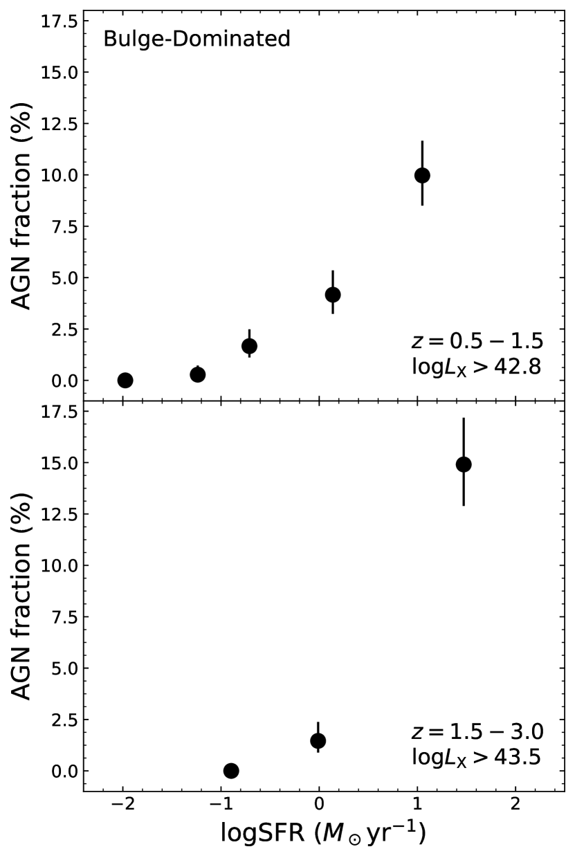
Considering the importance of SMBH-galaxy growth among bulge-dominated galaxies, we also plot AGN fraction as a function of SFR in Fig. 8. Here, we count an X-ray source as an “AGN” if it has () or (). These thresholds are the limits at and , respectively, for a keV flux limit of erg cm-2 s-1. This flux limit is the detection limit of the COSMOS survey (Civano et al., 2016), which is the shallowest CANDELS X-ray survey (Tab. 1). is mainly driven by duty cycle and average accretion rate of AGNs. From Fig. 8,666We cannot derive reliable average AGN X-ray luminosities and thereby accretion rates due to the small AGN sample sizes in most bins (see Tab. 3). AGN fraction increases toward high SFR for both redshift bins. This result indicates that the positive -SFR relation is, at least partially, due to the rise of AGN duty cycle toward high SFR. Detailed quantitative analyses of AGN duty cycle and average accretion rate require the full distribution of BHAR (see §2.4), for which we leave to future studies.
| Bulge-Dominated; | |||||
|---|---|---|---|---|---|
| Gal. # | X. # | AGN # | |||
| (1) | (2) | (3) | (4) | (5) | (6) |
| 10.24 | 360 | 14 | 0 | ||
| 10.44 | 360 | 20 | 1 | ||
| 10.48 | 360 | 29 | 6 | ||
| 10.25 | 360 | 46 | 15 | ||
| 10.19 | 361 | 69 | 36 | ||
| Bulge-Dominated; | |||||
| Gal. # | X. # | AGN # | |||
| (1) | (2) | (3) | (4) | (5) | (6) |
| 10.62 | 274 | 7 | 0 | ||
| 10.64 | 274 | 21 | 4 | ||
| 10.59 | 275 | 77 | 41 | ||
Note. — (1) & (2) Median and . (3) and its uncertainties. (4) Number of galaxies. (5) Number of X-ray sources. (6) Number of AGNs as defined in Fig. 8.
3.4 Reliability Checks
Our and SFR measurements are mostly based on SED fitting of rest-frame UV-to-NIR photometry, and we have removed BL AGNs from our sample to avoid strong AGN SED components that might affect our results (§2.2 and §3.3). Also, from Fig. 2, the X-ray detected sources do not appear to have strong central point-like emission, indicating that the presence of AGNs should not significantly affect the , SFR, and morphology measurements. On the other hand, if potential AGN SED contamination significantly biased our analyses, we would expect to reach a similar conclusion for bulge-dominated and comparison samples, which is not the case (§3.2). Therefore, we consider that our conclusions are not biased by AGN SED contamination. In §2.2, we have also discussed the SFR uncertainties of SED-based and FIR-based measurements, and found that our main conclusions are unlikely to be affected by those uncertainties.
Our bulge-dominated galaxies at are selected utilizing machine-learning morphological measurements based on HST -band imaging (§2.1 and §2.3). Morphological measurements at high redshift are challenging due to effects such as redshifting of photons and image degradation (e.g. Conselice 2014 and references therein). Detailed assessment of these redshift effects on our results requires careful simulations of HST imaging and repetition of the machine-learning measurements on the simulated data. These procedures are beyond the scope of this work. Here, we qualitatively discuss the robustness of our results against such redshift effects.
Due to the redshifting of photons, the same observed-frame wavelength covers different rest-frame wavelengths at different redshifts. The correction for this redshifting effect is named the “morphological -correction”. From multiwavelength observations of local galaxies, Taylor-Mager et al. (2007) found that the morphological -correction is weak in the optical/NIR wavelength range ( m, where m corresponds to the Balmer break and m is the longest wavelength available in their work), especially for elliptical/S0 galaxies. For our work, the observed-frame band (used for morphological measurements; §2.1) does not reach out to rest-frame UV photons below the Balmer break at , and it corresponds to the rest-frame NIR (m) and optical (m) light at and , respectively. Also, considering that we only utilize the morphological information for a basic selection of bulge-dominated galaxies rather than, e.g. a quantitative measurement of galaxy size, we conclude that the morphological -correction should not affect our results qualitatively. Another point of support for this conclusion is that, although the band is sampling different wavelengths for and , we have obtained qualitatively the same results for the two redshift bins (§3.2).
At low redshift, the band samples rest-frame red optical/NIR photons. Since galactic-disk components are generally bluer than bulge components, one might worry that -band imaging could miss disk components. This issue mainly happens for low- faint disky galaxies. Considering that our main focus is relatively massive galaxies (§2.3) and that CANDELS -band data are deep, this issue might not be problematic for our study. However, we still check this issue in the following ways. First, we visually check HST -band cutouts of random galaxies in our bulge-dominated samples at . We do not find significant disk components for these sources. Indeed, the average -band Sérsic index of our low-redshift bulge-dominated sample is (using the measurements of Scarlata et al. 2007), which is typical for bulge-dominated galaxies (e.g. Buitrago et al., 2013; Conselice, 2014). On the other hand, we visually check the low-redshift disky (; §2.3) galaxies in our sample. We find their disk components do not appear to be significantly weaker in band than in band, and we attribute this result to the deep exposure and relatively low extinction of band. Therefore, we consider that the band-based morphological classification is robust at low redshift.
The imaging quality generally becomes worse toward higher redshift. Some fine galactic structures (e.g. spiral arms and clumps) might be smoothed out, and thus some disky and irregular galaxies might be classified as the smooth bulge-dominated type (e.g. Mortlock et al. 2013). Therefore, our bulge-dominated sample might be “contaminated”. However, this issue is, at least to some extent, mitigated by the mag cut () applied to our sample (§2.1). This cut guarantees a minimum signal-to-noise ratio (S/N ) of the imaging, with the penalty of a smaller sample size. Also, if our bulge-dominated sample were strongly contaminated, we would observe a similar -SFR- relation for both the bulge-dominated and comparison samples. However, the dependences on SFR and are qualitatively different for these two samples (§3.2). We thus consider that image degradation should not be a significant issue for our conclusions.
4 Discussion
4.1 Physical Implications
We emphasize that the -SFR correlation only exists for our bulge-dominated sample, while appears to be primarily correlated with for the comparison sample. This difference indicates that SMBHs only coevolve with bulges rather than entire galaxies, consistent with the observations of local systems (e.g. Kormendy & Ho, 2013; Davis et al., 2018). Such SMBH-bulge coevolution might be driven by the amount of cold gas available in the bulge, since both SMBH and bulge growth require cold gas. From the SMBH-bulge coevolution scenario, we expect that is also fundamentally correlated with bulge SFR even when a galactic disk is present.
Earlier studies speculated an intrinsic -SFR relation for the overall galaxy population (see §1). However, the scenario of SMBH vs. entire galaxy coevolution leads to being strongly related to rather than in the local universe, contradicting observations (e.g. Kormendy & Ho, 2013). To reconcile this contradiction, an ad hoc galaxy evolution model was invoked where all stellar mass formed in the distant universe () is transformed to bulge mass at (Jahnke et al., 2009; Mullaney et al., 2012). In contrast, the -bulge SFR correlation, as revealed by our work, can naturally result in the - relation observed in the local universe, without invoking any unphysical galaxy evolution models. Our findings highlight the critical role of morphological measurements when observationally studying the connections between distant SMBHs and their host galaxies, as the -SFR correlation only exists among bulge-dominated galaxies. Without deep HST observations of CANDELS, our discovery would not be possible (see Appendix A).
Some papers attribute the local - relation entirely to a non-causal statistical origin (e.g. Peng 2007; Jahnke & Macciò 2011). If galaxy/SMBH mergers happen frequently enough, the scatter of the - relation could be averaged out. Our results show that there is indeed an intrinsic -SFR connection at high redshift that can lead to the - correlation among nearby galaxies (§4.2). Therefore, the non-causal scenarios of merger averaging are not necessary to explain the - relation. Also, recent observations of Yang et al. (2018a) show that frequent mergers will lead to a ratio much smaller than the observed values in the local universe.
Kocevski et al. (2017) found that, for compact galaxies, the star-forming population has elevated AGN fraction compared to the quiescent population with matched at . However, for extended galaxies, the star-forming and quiescent populations have similar AGN fractions. Since our bulge-dominated population is morphologically more compact than other galaxy populations in general (see Fig. 2; e.g. Huertas-Company et al. 2015a), our results in Fig. 6 are broadly consistent with the findings of Kocevski et al. (2017). While we consider our results as evidence of SMBH-bulge coevolution, Kocevski et al. (2017) argued that a contraction process might trigger both compact starburst activity and SMBH accretion. In our scenario, bulge SFR is fundamentally correlated with ; in their scenario, compactness is a critical galaxy property linked with SMBH growth. To address the question of which scenario is more physical, one needs to break the degeneracy that bulge-dominated systems are generally compact. We will perform these analyses in a future paper (Ni et al. in prep.).
4.2 Implications for the - Relation
From the best-fit results in §3.3, we have . This value is similar to the typical observed values in the local universe (; Kormendy & Ho 2013). Also, similar to the observed - relation in the local universe, our -SFR relation for bulge-dominated galaxies has slope close to unity. These similarities indicate that the observed - relation originates from SMBH-bulge coevolution as revealed by our work, and the - relation is not heavily biased by the possibility that observations tend to select massive SMBHs for measurements (e.g. Shankar et al., 2016).
The strong -SFR relation among bulge-dominated galaxies indicates that SMBH and bulge growth are in lockstep. A natural consequence from this lockstep growth is that the - relation should not have strong redshift dependence. Some observations suggest that the ratio appears to be higher toward higher redshifts (e.g. Shields et al., 2006; Ho, 2007), contradicting the scenario of lockstep growth. However, this apparent redshift dependence of might result from observational biases (e.g. Lauer et al., 2007), because measurements in the distant universe are generally limited to luminous quasars. These luminous quasars are likely the most massive SMBHs accreting at high Eddington ratios, and thus the observed should be systematically higher than the typical among the entire galaxy population.
4.3 Galaxies that are Not Bulge-Dominated
For our bulge-dominated sample, is fundamentally related to SFR. In contrast, for our comparison sample consisting of galaxies that are not bulge-dominated (§2.3), is not strongly coupled with SFR (§3.2), likely due to the fact that their total SFR is mostly contributed by non-bulge components. Actually, most () of the comparison galaxies are irregular/disk-dominated galaxies with no significant bulge components (; §2.3). The rest () of the population in the comparison sample is bulge-disk systems. For these systems, according to the SMBH-bulge coevolution scenario, should be intrinsically correlated with bulge SFR (§4.1).
For our comparison sample, is strongly related to (§3.2). The implications of this - relation are discussed in detail by Yang et al. (2018a),777Although Yang et al. (2018a) focused on the - relation for the entire galaxy population, their conclusions should largely hold for our comparison galaxies which are numerically the main population (; §2.3 and Appendix A). and we only summarized their main points below. Yang et al. (2018a) found that / rises toward high , i.e. massive galaxies are more effective in feeding their SMBHs (see their §4.2). This result inevitably leads to a higher ratio for more massive galaxies in the local universe, i.e. the typical local - relation should be non-linear (see their §4.3 and §4.4). On the other hand, Yang et al. (2018a) also considered that the local - relation might not be tight due to different stellar-mass histories of local galaxies with similar (see their §3.4.1). This is because is higher toward high redshift, at a given (see their Fig. 9). Therefore, for two galaxies with similar in the local universe, the one that forms at higher redshift should have a more massive SMBH.
5 Summary and Future Work
We have studied the dependence on SFR and for a bulge-dominated sample and a comparison sample of galaxies, respectively, based on multiwavelength observations of the CANDELS fields. Our main analysis procedures and conclusions are summarized below:
-
1.
We have compiled redshift, , and SFR for galaxies brighter than from the CANDELS catalogs (§2.2). The CANDELS and SFR measurements are based on SED fitting. For sources detected by Herschel, we estimate their SFR from FIR photometry. We have applied cuts of () and () to our sample to ensure completeness (§2.3). Based on machine-learning morphological measurements (§2.1), we have selected a sample of bulge-dominated galaxies and included the other galaxies in a comparison sample (§2.3). The bulge-dominated galaxies consist of of the entire galaxy population.
-
2.
We have measured sample-averaged BHAR for different samples of galaxies based on the deep X-ray observations from Chandra (§2.4). We first measure the for each X-ray detected source as well as average X-ray luminosity for undetected sources via a stacking process. From these measurements, we calculate average AGN bolometric luminosity adopting an -dependent bolometric correction. Finally, we estimate from assuming a constant radiation efficiency.
-
3.
For the bulge-dominated sample, we have shown, with both qualitative and quantitative (PCOR) analyses, that primarily depends on SFR rather than (§3.1 and §3.2). For the comparison sample, the situation is the opposite. The tight -SFR connection for bulge-dominated galaxies indicates that SMBHs only coevolve with bulges rather than entire host galaxies (S§4.1). The non-causal scenarios of merger averaging are unlikely the origin of the - relation in the local universe.
-
4.
Our best-fit -SFR relation for the bulge-dominated sample is where the slope is fixed to unity (§3.3). Our best-fit /SFR ratio is similar to the observed ratio in the local universe (§4.2). This agreement indicates that our observed -SFR relation is indeed responsible for the well-known tight - correlation among local galaxies. On the other hand, our findings support that the observed local - relation is not heavily biased. The strong -SFR relation among bulge-dominated galaxies indicate lockstep growth of SMBHs and bulges, predicting that the - relation should not have strong redshift dependence.
This paper probes the redshift range of . Future studies can extend our work down to using the 2 deg2 COSMOS field, or even to the local universe (e.g. Goulding et al., 2017) based on wide surveys, e.g. XMM-XXL (Pierre et al., 2016), Stripe 82X (LaMassa et al., 2016), XMM-SERVS (Chen et al., 2018), and the Chandra Source Catalog (Evans et al., 2010). Compared to distant systems in deep fields, local sources have the advantages of larger sample sizes and more accurate morphological measurements, and these advantages could reduce the uncertainties of the -SFR relation significantly. In the near future, we will also investigate whether bulge SFR or galaxy compactness is more tightly linked to SMBH growth (Ni et al. in prep.; §4.1). Future work could furthermore derive the full BHAR distribution as a function of SFR and for bulge-dominated and comparison galaxies, respectively, and detailed sample properties such as duty cycle and average accretion rate of AGNs can be further obtained and analyzed (§2.4 and Fig. 8). However, such studies will require a large galaxy sample with reliable morphological measurements, and thus deep HST (or future JWST and WFIRST) imaging over much larger fields than CANDELS is needed.
Since our results indicate that SMBHs grow in lockstep with host-galaxy bulges, we also expect a strong connection between and bulge SFR for systems that have both bulge and disk components (§4.1 and §4.3). Future ALMA observations could study the -bulge SFR connection among these systems. ALMA can cover FIR wavelengths down to observed-frame m, corresponding to the typical SED-peak wavelength (m, rest-frame) of cold-dust emission of galaxies at . Therefore, IR luminosities and thereby FIR-based SFR can be reliably estimated for these systems with ALMA. Since ALMA can reach HST-like resolutions, it should be able to separate reliably bulge SFR from total SFR. The strong -SFR connection among bulge-dominated galaxies might be physically driven by the amount of cold gas available (see §4.1). To test this idea, one could compare the gas masses of high-SFR vs. low-SFR bulge-dominated galaxies with observations by ALMA. ALMA could measure gas masses by observing the CO lines. ALMA could also observe the Rayleigh–Jeans tail of cold dust emission (m, rest-frame), which is a reliable tracer of dust masses (e.g. Scoville et al., 2017). Gas masses can then be estimated from dust masses with the assumption of a typical dust-to-gas ratio, although uncertainties inevitably exist in this conversion (e.g. Simpson et al., 2015).
Appendix A Results for All Galaxies
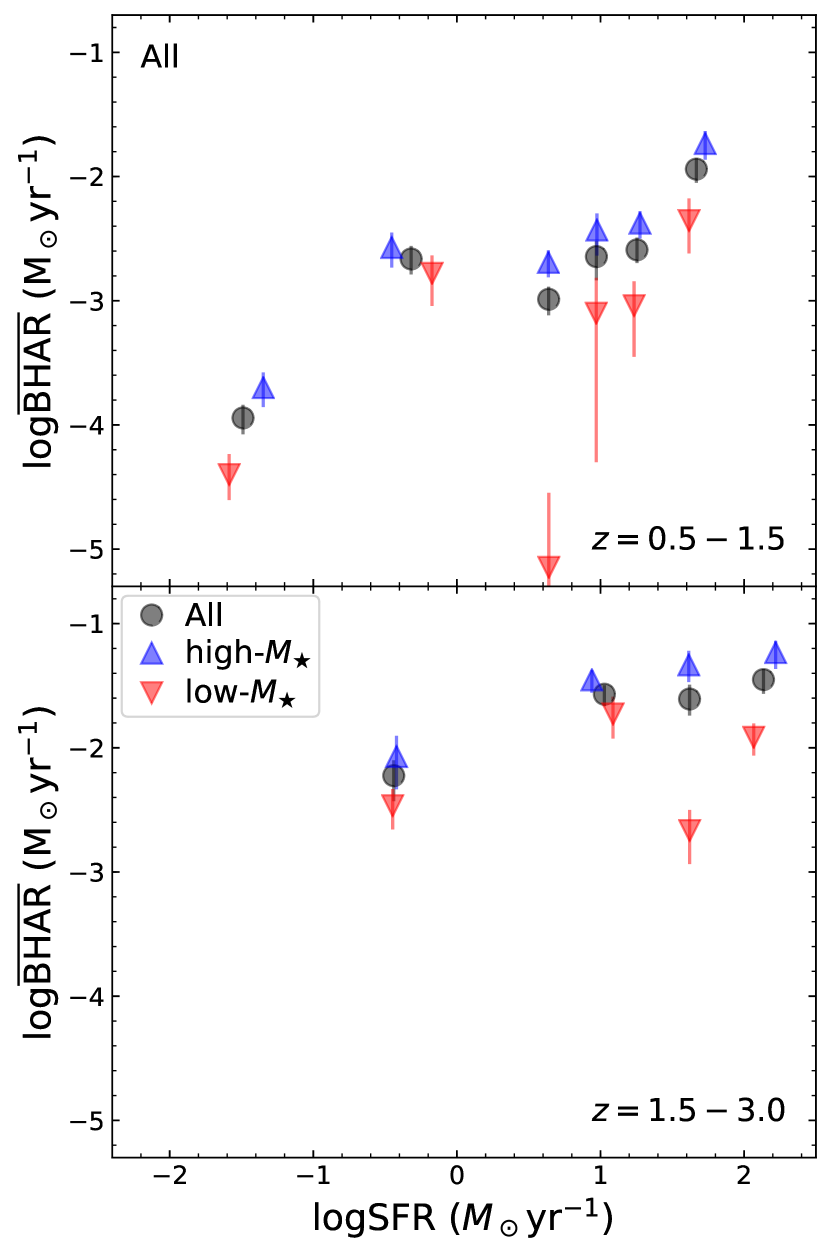
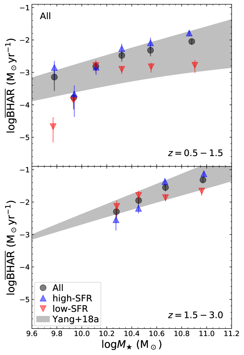
In this appendix, we perform analyses like those in §3 for all galaxies with , including both the bulge-dominated and comparison samples grouped together. The results are presented in Figs. 9, 10, and 11, and Tab. 4. In Fig. 10, we also compare the - relation with that derived in Yang et al. (2018a). The - relation in this work agrees with the results of Yang et al. (2018a).
From Tab. 4, is more strongly related to than SFR. This is expected, because the comparison sample is the numerically dominant galaxy population (see §2.3) and is mainly related to for the comparison sample, especially at . This conclusion is also qualitatively consistent with Yang et al. (2017), although their statistical significances of the - relation are higher than those in Tab. 4. We attribute this difference to the fact that the dynamic range of probed in Yang et al. (2017) is much wider than that in this work ( vs. ), since here we require to ensure high-quality morphological information for all galaxies. The narrower dynamic range also results in smaller sample sizes, leading to the relatively large statistical scatter in Figs. 9 and 10 (compared to Figs. 4 and 5 in Yang et al. 2017).
| All; | ||
|---|---|---|
| Relation | Pearson | Spearman |
| - | () | () |
| - | () | () |
| All; | ||
| Relation | Pearson | Spearman |
| - | () | () |
| - | () | () |
Acknowledgements
We thank the referee for helpful feedback that improved this work. We thank Robin Ciardullo, Mara Salvato, Ian Smail, Yongquan Xue, and Wenfei Yu for helpful discussions. GY, WNB, and QN acknowledge support from Chandra X-ray Center grant AR8-19016X, NASA grant NNX17AF07G, NASA ADP grant 80NSSC18K0878, and the V.M. Willaman Endowment. The Chandra Guaranteed Time D.M.A. acknowledges the Science and Technology Facilities Council through grant ST/L00075X/1. FV acknowledge financial support from CONICYT and CASSACA through the Fourth call for tenders of the CAS-CONICYT Fund. Observations (GTO) for the GOODS-N were selected by the ACIS Instrument Principal Investigator, Gordon P. Garmire, currently of the Huntingdon Institute for X-ray Astronomy, LLC, which is under contract to the Smithsonian Astrophysical Observatory via Contract SV2-82024. This project uses Astropy (a Python package; see Astropy Collaboration et al. 2018).
References
- Aird et al. (2010) Aird J., et al., 2010, MNRAS, 401, 2531
- Aird et al. (2015) Aird J., Coil A. L., Georgakakis A., Nandra K., Barro G., Pérez-González P. G., 2015, MNRAS, 451, 1892
- Aird et al. (2018a) Aird J., Coil A. L., Georgakakis A., 2018a, arXiv e-prints,
- Aird et al. (2018b) Aird J., Coil A. L., Georgakakis A., 2018b, MNRAS, 474, 1225
- Astropy Collaboration et al. (2018) Astropy Collaboration et al., 2018, preprint, (arXiv:1801.02634)
- Azadi et al. (2015) Azadi M., et al., 2015, ApJ, 806, 187
- Barger et al. (2003) Barger A. J., et al., 2003, AJ, 126, 632
- Behroozi et al. (2013) Behroozi P. S., Wechsler R. H., Conroy C., 2013, ApJ, 770, 57
- Brandt & Alexander (2015) Brandt W. N., Alexander D. M., 2015, A&ARv, 23, 1
- Buat et al. (2010) Buat V., et al., 2010, MNRAS, 409, L1
- Buitrago et al. (2013) Buitrago F., Trujillo I., Conselice C. J., Häußler B., 2013, MNRAS, 428, 1460
- Chabrier (2003) Chabrier G., 2003, ApJ, 586, L133
- Chen et al. (2013) Chen C.-T. J., et al., 2013, ApJ, 773, 3
- Chen et al. (2018) Chen C.-T. J., et al., 2018, MNRAS, 478, 2132
- Civano et al. (2016) Civano F., et al., 2016, ApJ, 819, 62
- Conselice (2014) Conselice C. J., 2014, ARA&A, 52, 291
- Cooper et al. (2012) Cooper M. C., et al., 2012, MNRAS, 425, 2116
- Dai et al. (2018) Dai Y. S., Wilkes B. J., Bergeron J., Kuraszkiewicz J., Omont A., Atanas A., Teplitz H. I., 2018, MNRAS, 478, 4238
- Davidzon et al. (2017) Davidzon I., et al., 2017, A&A, 605, A70
- Davis et al. (2018) Davis B. L., Graham A. W., Cameron E., 2018, preprint, (arXiv:1810.04888)
- Evans et al. (2010) Evans I. N., et al., 2010, ApJS, 189, 37
- Ferrarese & Merritt (2000) Ferrarese L., Merritt D., 2000, ApJ, 539, L9
- Fornasini et al. (2018) Fornasini F. M., Civano F., Fabbiano G., Elvis M., Marchesi S., Miyaji T., Zezas A., 2018, ApJ, 865, 43
- Fragos et al. (2013) Fragos T., et al., 2013, ApJ, 764, 41
- Galametz et al. (2013) Galametz A., et al., 2013, ApJS, 206, 10
- Gebhardt et al. (2000) Gebhardt K., et al., 2000, ApJ, 539, L13
- Georgakakis et al. (2014) Georgakakis A., et al., 2014, MNRAS, 443, 3327
- Georgakakis et al. (2017) Georgakakis A., Aird J., Schulze A., Dwelly T., Salvato M., Nandra K., Merloni A., Schneider D. P., 2017, MNRAS, 471, 1976
- Goulding et al. (2012) Goulding A. D., et al., 2012, ApJS, 202, 6
- Goulding et al. (2017) Goulding A. D., et al., 2017, ApJ, 843, 135
- Grogin et al. (2011) Grogin N. A., et al., 2011, ApJS, 197, 35
- Guo et al. (2013) Guo Y., et al., 2013, ApJS, 207, 24
- Häring & Rix (2004) Häring N., Rix H.-W., 2004, ApJ, 604, L89
- Harrison et al. (2012) Harrison C. M., et al., 2012, ApJ, 760, L15
- Hickox et al. (2014) Hickox R. C., Mullaney J. R., Alexander D. M., Chen C.-T. J., Civano F. M., Goulding A. D., Hainline K. N., 2014, ApJ, 782, 9
- Ho (2007) Ho L. C., 2007, ApJ, 669, 821
- Hopkins et al. (2007) Hopkins P. F., Richards G. T., Hernquist L., 2007, ApJ, 654, 731
- Huertas-Company et al. (2015a) Huertas-Company M., et al., 2015a, ApJS, 221, 8
- Huertas-Company et al. (2015b) Huertas-Company M., et al., 2015b, ApJ, 809, 95
- Huertas-Company et al. (2016) Huertas-Company M., et al., 2016, MNRAS, 462, 4495
- Ilbert et al. (2013) Ilbert O., et al., 2013, A&A, 556, A55
- Jahnke & Macciò (2011) Jahnke K., Macciò A. V., 2011, ApJ, 734, 92
- Jahnke et al. (2009) Jahnke K., et al., 2009, ApJ, 706, L215
- Kartaltepe et al. (2015) Kartaltepe J. S., et al., 2015, ApJS, 221, 11
- Kelly et al. (2010) Kelly B. C., Vestergaard M., Fan X., Hopkins P., Hernquist L., Siemiginowska A., 2010, ApJ, 719, 1315
- Kim (2015) Kim S., 2015, Communications for statistical applications and methods, 22, 665
- Kirkpatrick et al. (2012) Kirkpatrick A., et al., 2012, ApJ, 759, 139
- Kocevski et al. (2017) Kocevski D. D., et al., 2017, ApJ, 846, 112
- Kocevski et al. (2018) Kocevski D. D., et al., 2018, ApJS, 236, 48
- Koekemoer et al. (2011) Koekemoer A. M., et al., 2011, ApJS, 197, 36
- Kormendy & Ho (2013) Kormendy J., Ho L. C., 2013, ARA&A, 51, 511
- LaMassa et al. (2016) LaMassa S. M., et al., 2016, ApJ, 817, 172
- Lanzuisi et al. (2017) Lanzuisi G., et al., 2017, A&A, 602, A123
- Lauer et al. (2007) Lauer T. R., Tremaine S., Richstone D., Faber S. M., 2007, ApJ, 670, 249
- Leauthaud et al. (2015) Leauthaud A., et al., 2015, MNRAS, 446, 1874
- Lehmer et al. (2016) Lehmer B. D., et al., 2016, ApJ, 825, 7
- Liu et al. (2017) Liu T., et al., 2017, ApJS, 232, 8
- Luo et al. (2010) Luo B., et al., 2010, ApJS, 187, 560
- Luo et al. (2017) Luo B., et al., 2017, ApJS, 228, 2
- Lutz et al. (2011) Lutz D., et al., 2011, A&A, 532, A90
- Madau & Dickinson (2014) Madau P., Dickinson M., 2014, ARA&A, 52, 415
- Magnelli et al. (2013) Magnelli B., et al., 2013, A&A, 553, A132
- Magorrian et al. (1998) Magorrian J., et al., 1998, AJ, 115, 2285
- Marchesi et al. (2016) Marchesi S., et al., 2016, ApJ, 817, 34
- Marsan et al. (2018) Marsan Z. C., et al., 2018, preprint, (arXiv:1808.03284)
- Martig et al. (2009) Martig M., Bournaud F., Teyssier R., Dekel A., 2009, ApJ, 707, 250
- Martini (2004) Martini P., 2004, Coevolution of Black Holes and Galaxies, p. 169
- Mendez et al. (2016) Mendez A. J., et al., 2016, ApJ, 821, 55
- Merloni & Heinz (2013) Merloni A., Heinz S., 2013, Evolution of Active Galactic Nuclei. p. 503, doi:10.1007/978-94-007-5609-0_11
- Mortlock et al. (2013) Mortlock A., et al., 2013, MNRAS, 433, 1185
- Mullaney et al. (2012) Mullaney J. R., et al., 2012, ApJ, 753, L30
- Nandra et al. (2015) Nandra K., et al., 2015, ApJS, 220, 10
- Nayyeri et al. (2017) Nayyeri H., et al., 2017, ApJS, 228, 7
- Newman et al. (2013) Newman J. A., et al., 2013, ApJS, 208, 5
- Novak et al. (2011) Novak G. S., Ostriker J. P., Ciotti L., 2011, ApJ, 737, 26
- Oliver et al. (2012) Oliver S. J., et al., 2012, MNRAS, 424, 1614
- Peng (2007) Peng C. Y., 2007, ApJ, 671, 1098
- Pierre et al. (2016) Pierre M., et al., 2016, A&A, 592, A1
- Powell et al. (2018) Powell M. C., et al., 2018, ApJ, 858, 110
- Rodighiero et al. (2014) Rodighiero G., et al., 2014, MNRAS, 443, 19
- Rosario et al. (2013) Rosario D. J., et al., 2013, ApJ, 763, 59
- Santini et al. (2015) Santini P., et al., 2015, ApJ, 801, 97
- Sartori et al. (2018) Sartori L. F., Schawinski K., Trakhtenbrot B., Caplar N., Treister E., Koss M. J., Urry C. M., Zhang C. E., 2018, MNRAS, 476, L34
- Scarlata et al. (2007) Scarlata C., et al., 2007, ApJS, 172, 406
- Scoville et al. (2017) Scoville N., et al., 2017, ApJ, 837, 150
- Shankar et al. (2016) Shankar F., et al., 2016, MNRAS, 460, 3119
- Shields et al. (2006) Shields G. A., Salviander S., Bonning E. W., 2006, New Astron. Rev., 50, 809
- Silverman et al. (2010) Silverman J. D., et al., 2010, ApJS, 191, 124
- Simpson et al. (2015) Simpson J. M., et al., 2015, ApJ, 799, 81
- Stanley et al. (2015) Stanley F., Harrison C. M., Alexander D. M., Swinbank A. M., Aird J. A., Del Moro A., Hickox R. C., Mullaney J. R., 2015, MNRAS, 453, 591
- Stanley et al. (2017) Stanley F., et al., 2017, MNRAS, 472, 2221
- Stefanon et al. (2017) Stefanon M., et al., 2017, ApJS, 229, 32
- Symeonidis et al. (2016) Symeonidis M., Giblin B. M., Page M. J., Pearson C., Bendo G., Seymour N., Oliver S. J., 2016, MNRAS, 459, 257
- Taylor-Mager et al. (2007) Taylor-Mager V. A., Conselice C. J., Windhorst R. A., Jansen R. A., 2007, ApJ, 659, 162
- Tomczak et al. (2014) Tomczak A. R., et al., 2014, ApJ, 783, 85
- Ueda et al. (2014) Ueda Y., Akiyama M., Hasinger G., Miyaji T., Watson M. G., 2014, ApJ, 786, 104
- Vito et al. (2016) Vito F., et al., 2016, MNRAS, 463, 348
- Volonteri et al. (2015) Volonteri M., Capelo P. R., Netzer H., Bellovary J., Dotti M., Governato F., 2015, MNRAS, 452, L6
- Whitaker et al. (2012) Whitaker K. E., van Dokkum P. G., Brammer G., Franx M., 2012, ApJ, 754, L29
- Whitaker et al. (2017) Whitaker K. E., Pope A., Cybulski R., Casey C. M., Popping G., Yun M. S., 2017, ApJ, 850, 208
- Wuyts et al. (2011) Wuyts S., et al., 2011, ApJ, 738, 106
- Xue et al. (2016) Xue Y. Q., Luo B., Brandt W. N., Alexander D. M., Bauer F. E., Lehmer B. D., Yang G., 2016, ApJS, 224, 15
- Yang et al. (2016) Yang G., et al., 2016, ApJ, 831, 145
- Yang et al. (2017) Yang G., et al., 2017, ApJ, 842, 72
- Yang et al. (2018a) Yang G., et al., 2018a, MNRAS, 475, 1887
- Yang et al. (2018b) Yang G., Brandt W. N., Darvish B., Chen C.-T. J., Vito F., Alexander D. M., Bauer F. E., Trump J. R., 2018b, MNRAS, 480, 1022