Quantifying high-order interdependencies
via multivariate extensions of the mutual information

Abstract

This article introduces a model-agnostic approach to study statistical synergy, a form of emergence in which patterns at large scales are not traceable from lower scales. Our framework leverages various multivariate extensions of Shannon’s mutual information, and introduces the O-information as a metric capable of characterising synergy- and redundancy-dominated systems. We develop key analytical properties of the O-information, and study how it relates to other metrics of high-order interactions from the statistical mechanics and neuroscience literature. Finally, as a proof of concept, we use the proposed framework to explore the relevance of statistical synergy in Baroque music scores.

I Introduction

A unique opportunity in the era of “big data” is to make use of the abundant data to deepen our understanding of the high-order interdependencies that are at the core of complex systems. Plentiful data is nowadays available about e.g. the orchestrated activity of multiple brain areas, the relationship between various econometric indices, or the interactions between different genes. What allows these systems to be more than the sum of their parts is not in the nature of the parts, but in the structure of their interdependencies crutchfield1994calculi . However, quantifying the “synergy” within a given set of interdependencies is challenging, especially in scenarios where the number of parts is far below the thermodynamic limit.

The relevance of synergistic relationships related to high-order interactions has been thoughtfully demonstrated in the theoretical neuroscience literature. For example, studies on neural coding have shown that neurons can carry redundant, complementary or synergistic information – the latter corresponding to neurons that are uninformative individually but informative when considered together schneidman2003synergy ; latham2005synergy . Also, studies on retina cells suggest that high-order Hamiltonians are necessary for representing neurons firing in response to natural images, while pairwise interactions suffice for neurons responding to less structured stimuli ganmor2011sparse . Lastly, neuroimaging analyses have pointed out the compatibility of local differentiation and global integration of different brain areas, and suggested this to be a key capability for enabling high cognitive functions tononi1998complexity ; balduzzi2008integrated . Various metrics have been proposed to distinguish these high-order features in data, including the redundancy-synergy index gat1999synergy ; chechik2002group ; varadan2006computational , connected information schneidman2003network , neural complexity tononi1994measure , and integrated information barrett2011practical ; mediano2018measuring . While being capable of capturing features of biological relevance, most of these metrics have ad hoc definitions motivated by specific research agendas, and have few theoretical guarantees .

A promising approach for addressing high-order interdependencies is partial information decomposition (PID), which distinguishes different “types” of information that multiple predictors convey about a target variable williams2010nonnegative ; griffith2014quantifying ; wibral2017partial . In this framework, statistical synergies are structures (or relationships) that exist in the whole but cannot be seen in the parts, being this rooted in the elementary fact that variables can be pairwise independent while being globally correlated. Unfortunately, the adoption of PID has been hindered by the lack of agreement on how to compute the components of the decomposition, despite numerous recent efforts barrett2015exploration ; ince2017measuring ; james2018unique ; finn2018pointwise . Moreover, the practical value of PID is greatly limited by the super-exponential growth of terms for large systems, although some applications do exist tax2017partial ; wibral2017quantifying .

The crux of multivariate interdependencies is that information-theoretic descriptions of such phenomena are not straighforward, as extensions of Shannon’s classical results to general multivariate settings have proven elusive el2011network . The most well-established multivariate extensions of Shannon’s mutual information are the total correlation watanabe1960information and the dual total correlation han1975linear , which provide suitable metrics of overall correlation strength. Their values, however, differ in ways that are hard to understand, even gaining the adjective of “enigmatic” among scholars james2011anatomy ; vijayaraghavan2017anatomy . Other popular extension of the mutual information is the interaction information mcgill1954multivariate , which is a signed measure obtained by applying the inclusion-exclusion principle to the Shannon entropy ting1962 ; yeung1991 . Although this metric provides insighful results when applied to three variables, its is not easily interpretable when applied to larger groups williams2010nonnegative .

This paper proposes to study multivariate interdependency via two dual persectives: as shared randomness and as collective constraints . This setup leads to the O-information, which – following Occam’s razor – points out which of these perspectives provides a more parsimonious description of the system. The O-information is found to coincide with the interaction information for the case of three variables, while providing a more meaningful extension for larger system sizes.

We show how the O-information captures the dominant characteristic of multivariate interdependency, distinguishing redundancy-dominated scenarios where three or more variables have copies of the same information, and synergy-dominated systems characterised by high-order patterns that cannot be traced from low-order marginals. In contrast with existing quantities that require a division between predictors and target variables, the O-information is – to the best of our knowledge – the first symmetric quantity that can give account of intrinsic statistical synergy in systems of more than three parts. Moreover, the computational complexity of the O-information scales gracefully with system size, making it suitable for practical data analysis.

In the sequel, Section II introduces the notions of shared randomness and collective constraints, and Sections III and IV present the O-information and its fundamental properties. Section V compares the O-information with other metrics of high-order effects, and Section VI presents a case study on music scores. Finally, Section VII summarises our main conclusions.

II Fundamentals

This section introduces two fundamental perspectives from which one can develop an information-theoretic description of a system, and explains how they enable novel perspectives to study interdependency.

II.1 Entropy and negentropy

For every outside there is an inside and for every inside there is an outside. And although they are different, they always go together.

Alan Watts, Myth of myself

Following the Bayesian interpretation of information theory, we define the information contained in a system as the amount of data that an observer would gain after determining its configuration – i.e. after measuring it jaynes2003probability . If each possible configuration is to be represented by a distinct sequence of bits, source coding theory (cover2012elements, , Ch. 5) shows that an optimal (i.e. shortest) labelling depends on prior information available before the measurement. Information, hence, refers to how the state of knowledge of the observer changes after the system is measured, quantifying the amount of bits that are revealed through this process .

Let us consider an observer measuring a system composed by $n$ discrete variables, $\bm{X}^{n}=(X_{1},\dots,X_{n})$. If the observer only knows that each variable $X_{j}$ can take values over a finite alphabet $\mathcal{X}_{j}$ of cardinality $|\mathcal{X}_{j}|$, the amount of information needed to specify the state of $X_{j}$ is $\log|\mathcal{X}_{j}|$ (logarithms are calculated using base $2$ unless specified otherwise). In contrast, if the observer knows that the system’s behaviour follows a probability distribution $p_{\bm{X}^{n}}$, then the average amount of information in the system reduces to the entropy $H(\bm{X}^{n})\coloneqq-\sum_{\bm{x}^{n}}p_{\bm{X}^{n}}(\bm{x}^{n})\log p_{\bm{X}^{n}}(\bm{x}^{n})$ jaynes2003probability . The difference

$$\mathcal{N}(\bm{X}^{n})\coloneqq\sum_{j=1}^{n}\log|\mathcal{X}_{j}|-H(\bm{X}^{n})$$ (1)

is known as negentropy brillouin1953negentropy , and corresponds to the information about the system that is disclosed by its statistics, before any measurement takes place.

Probability distributions are, from this perspective, a compendium of soft and hard constraints that reduce the effective phase space that the system can explore – hard constraints completely forbid some configurations, while soft constraints make them improbable. Consequently, a given distribution divides the phase space in an admisible region quantified by the entropy, and an inadmissible region quantified by the negentropy . Each part describes the system’s structure from a different point of view: the entropy refers to what the system can do, while the negentropy refers to what it can’t.

II.2 The two faces of interdependency

II.2.1 Collective constraints

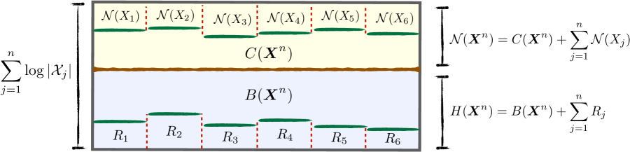
Figure 1: Following Eq. (4), the total information that can be stored in the system $\bm{X}^{n}$ ($\sum_{j=1}^{n}\log|\mathcal{X}_{j}|$) is divided by a given state of knowledge (i.e. a probability distribution) into what is determined by the constraints ($\mathcal{N}(\bm{X}^{n})$) and what is not instantiated until an actual measurement takes place ($H(\bm{X}^{n})$). Moreover, both terms can be further decomposed into their individual and collective components, yielding different perspectives on interdependency seen as either collective constraints ($C(\bm{X}^{n})$) or shared randomness ($B(\bm{X}^{n})$).

In the same way as $\mathcal{N}(\bm{X}^{n})$ quantifies the strength of the overall constraints that rule the system, the constraints that affect individual variables are captured by the marginal negentropies $\mathcal{N}(X_{j})\coloneqq\log|\mathcal{X}_{j}|-H(X_{j})$. Intuitively, the constraints that affect the whole system are richer than individual constraints, as the latter do not take into account collective effects. Their difference,

$$\begin{split}C(\bm{X}^{n})\coloneqq&\;\mathcal{N}(\bm{X}^{n})-\sum_{j=1}^{n}\mathcal{N}(X_{j})\\ =&\sum_{j=1}^{n}H(X_{j})-H(\bm{X}^{n})~{},\end{split}$$ (2)

quantifies the strength of the “collective constraints.” This quantity is known as total correlation watanabe1960information (or multi-information studeny1998multiinformation ). By re-writing this relationship as $\mathcal{N}(\bm{X}^{n})=\sum_{j}\mathcal{N}(X_{j})+C(\bm{X}^{n})$ one finds that the constraints prescribed by the distribution are of two types: constraints confined to individual variables, and collective constraints that restrict groups of two or more variables.

Example 1.

Consider $X_{1}$ and $X_{2}$ to be binary random variables with $p_{X_{1},X_{2}}(0,1)=p_{X_{1},X_{2}}(1,0)=1/2$. This distribution divides the total information (two bits) into $H(X_{1},X_{2})=1$ and $\mathcal{N}(X_{1},X_{2})=1$ . Moreover, $\mathcal{N}(X_{1})=\mathcal{N}(X_{2})=0$ and therefore $C(X_{1},X_{2})=\mathcal{N}(X_{1},X_{2})=1$, confirming that the constraints act on both $X_{1}$ and $X_{2}$.

As a contrast, consider $Y_{1}$ and $Y_{2}$ binary random variables with distribution $p_{Y_{1},Y_{2}}(0,0)=p_{Y_{1},Y_{2}}(1,0)=1/2$. In this case $\mathcal{N}(Y_{1})=0$ while $\mathcal{N}(Y_{2})=\mathcal{N}(Y_{1},Y_{2})=1$, showing that the only constraint in this system acts solely over $Y_{2}$. Accordingly, for this case $C(Y_{1},Y_{2})=0$.

II.2.2 Shared randomness

As we did for $\mathcal{N}(\bm{X}^{n})$, let us decompose $H(\bm{X}^{n})$ in individual and collective components. To do this, we introduce the quantity $R_{j}=H(X_{j}|\bm{X}_{-j}^{n})$ as a metric of how independent $X_{j}$ is from the rest of the system $\bm{X}^{n}_{-j}=(X_{1},\dots,X_{j-1},X_{j+1},\dots,X_{n})$. According to distributed source coding theory (el2011network, , Ch. 10.5), $R_{j}$ corresponds to the data contained in $X_{j}$ that cannot be extracted from measurements of other variables . The quantity $\sum_{j=1}^{n}R_{j}$ is known as the residual entropy abdallah2012measure (originally introduced under the name of erasure entropy verdu2006erasure ; verdu2008information ), and quantifies the total information that can only be accessed by measuring a specific variable, i.e. the amount of “non-shared randomness.” Accordingly, the difference

$$B(\bm{X}^{n})\coloneqq H(\bm{X}^{n})-\sum_{j=1}^{n}R_{j}$$ (3)

quantifies the amount of information that is shared by two or more variables – equivalently, information that can be accessed by measuring more than one variable. Although this quantity was introduced under the name of dual total correlation han1975linear (also known as excess entropy olbrich2008should or binding information abdallah2012measure ; vijayaraghavan2017anatomy ), we prefer the name binding entropy as it emphasises the fact that it is actually a part of the entropy. As the entropy corresponds to the randomness within the system, the binding entropy quantifies the “shared randomness” that exists among the variables.

Example 2.

Let us consider $X_{1},X_{2}$ and $Y_{1},Y_{2}$ from Example 1. For the former system one finds that $R_{1}=R_{2}=0$ and hence $B(X_{1},X_{2})=H(X_{1},X_{2})=1$, which means that the randomness within the system can be retrieved from measuring either $X_{1}$ or $X_{2}$. In contrast, when considering $Y_{1},Y_{2}$ one finds that $R_{2}=0$ and $R_{1}=H(Y_{1},Y_{2})=1$, and hence $B(Y_{1},Y_{2})=0$. This implies that the randomness of the system can be retrieved by measuring only $Y_{1}$.

Wrapping up, one can re-write Eq. (1) using Eqs. (2) and (3) and express the total information encoded in the system described by $\bm{X}^{n}$ in terms of constraints and randomness:

$$\begin{split}\sum_{j=1}^{n}&\log|\mathcal{X}_{j}|=\;\mathcal{N}(\bm{X}^{n})+H(\bm{X}^{n})\\ =&\underbrace{\left[C(\bm{X}^{n})+\sum_{j=1}^{n}\mathcal{N}(X_{j})\right]}_{\mathclap{\begin{subarray}{c}\mathrm{Collective~{}and~{}individual}\\[1.50694pt] \mathrm{constraints}\end{subarray}}}+\underbrace{\left[B(\bm{X}^{n})+\sum_{j=1}^{n}R_{j}\right]}_{\mathclap{\begin{subarray}{c}\mathrm{Shared~{}and~{}private}\\[1.50694pt] \mathrm{randomness}\end{subarray}}}.\end{split}$$ (4)

This decomposition is illustrated in Figure 1.

III Introducing the O-information

III.1 Definition and basic properties

The total correlation and the binding entropy provide complementary metrics of interdependence strength. Following Occam’s Razor, one might ask which of these perspectives allows for a shorter (i.e. more parsimonious) description. This is answered by the following definition:

Definition 1.

The O-information (shorthand for “information about Organisational structure”) of the system described by the random vector $\bm{X}^{n}$ is defined as

$$\Omega(\bm{X}^{n})\!\coloneqq \;C(\bm{X}^{n})-B(\bm{X}^{n})$$ (5)

$$= (n-2)H(\bm{X}^{n})+\sum_{j=1}^{n}\big{[}H(X_{j})-H(\bm{X}_{-j}^{n})\big{]}.$$

Intuitively, $\Omega(\bm{X}^{n})>0$ states that the interdependencies can be more efficiently explained as shared randomness, while $\Omega(\bm{X}^{n})<0$ implies that viewing them as collective constraints can be more convenient. Note that $\Omega(\bm{X}^{n})$ was first introduced as “enigmatic information” in Ref. james2011anatomy , although now that its properties have been revealed we choose to give it a more appropriate name.

To develop some insight about the O-information, let us compare it with the interaction information , which is a signed metric defined by

$$I(X_{1};X_{2};\dots;X_{n})\coloneqq-\sum_{\bm{\gamma}\subseteq\{1,\dots,n\}}(-1)^{|\bm{\gamma}|}H(\bm{X}^{\bm{\gamma}})~{},$$ (6)

where the sum is performed over all subsets $\bm{\gamma}\subseteq\{1,\dots,n\}$, with $|\bm{\gamma}|$ being the cardinality of $\bm{\gamma}$ and $\bm{X}^{\bm{\gamma}}$ the vector of all variables with indices in $\bm{\gamma}$. For $n=2$, Eq. (6) reduces to the well-known mutual information,

$$I(X_{1};X_{2})=H(X_{1})+H(X_{2})-H(X_{1},X_{2})~{}.$$

For $n=3$, Eq. (6) gives

$$I(X_{1};X_{2};X_{3})\! =I(X_{i};X_{j})-I(X_{i};X_{j}|X_{k})$$ (7)

$$=I(X_{i};X_{j})+I(X_{i};X_{k})-I(X_{i};X_{j},X_{k})$$

for $\{i,j,k\}=\{1,2,3\}$, which is known to measure the difference between synergy and redundancy williams2010nonnegative . Specifically, redundancy dominates when $I(X_{1};X_{2};X_{3})\geq 0$; e.g. if $X_{1}$ is a Bernoulli random variable with $p=1/2$ and $X_{1}=X_{2}=X_{3}$, then $I(X_{1};X_{2};X_{3})=1$. In contrast, synergy dominates when $I(X_{1};X_{2};X_{3})\leq 0$, corresponding to statistical structures that are present in the full distribution but not in the pairwise marginals. For example, if $Y_{1}$ and $Y_{2}$ are independent Bernoulli variables with $p=1/2$ and $Y_{3}=Y_{1}+Y_{2}\pmod{2}$ (i.e. an xor logic gate) then $I(Y_{1};Y_{2};Y_{3})=-1$, since these variables are pairwise independent while globally correlated rosas2016understanding . Unfortunately, for $n\geq 4$ the co-information no longer reflects the balance between redundancy and synergy (williams2010nonnegative, , Section V).

To contrast with the interaction information, the next Lemma presents some basic properties of $\Omega$ (the proofs are left for the reader).

Lemma 1.

The O-information satisfies the following properties:

• $\Omega$ does not depend on the order of $X_{1},\dots,X_{n}$.

• $\Omega(X_{1},X_{2})=0$ for any $p_{X_{1}X_{2}}$.

• $\Omega(X_{1},X_{2},X_{3})=I(X_{1};X_{2};X_{3})$ for any $p_{\bm{X}^{3}}$.

Property (A) shows that $\Omega$ reflects an intrinsic property of the system, without the need of dividing the variables in groups with differentiated roles (e.g. targets vs predictors, or input vs output). Property (B) confirms that $\Omega$ captures only interactions that go beyond pairwise relationships. Finally, Property (C) shows that when $n=3$ the O-information is equal to $I(X_{1};X_{2};X_{3})$. Interestingly, a direct calculation shows that if $n>3$ then in general $\Omega(\bm{X}^{n})\neq I(X_{1};X_{2};\dots;X_{n})$.

At this stage, one might wonder if the O-information could provide a metric for quantifying the balance of redundancy and synergy, as the interaction information does for $n=3$. Intutively, one could expect redundant systems to have small $B(\bm{X}^{n})$ due to the multiple copies of the same information that exist in the system, while having large values of $C(\bm{X}^{n})$ because of the constraints that are needed to ensure that the variables remain correlated. On the other hand, synergistic systems are expected to have small values of $C(\bm{X}^{n})$ due to the few high-order constraints that rule the system, while having larger values of $B(\bm{X}^{n})$ due to the weak low-order structure. These insights are captured in the following definition, which is supported by multiple findings presented in the following sections.

Definition 2.

If $\Omega(\bm{X}^{n})>0$ we say that the system is redudancy-dominated, while if $\Omega(\bm{X}^{n})<0$ we say it is synergy-dominated.

In previous work we used another metric to assess synergy- and redundancy-dominated systems rosas2018selforg . Appendix A provides an analytical and numerical account of the consistency between these two metrics.

III.2 Information decompositions

III.2.1 The lattice of partitions

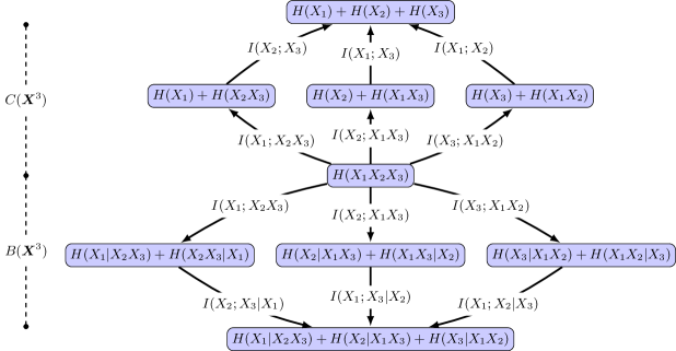
Figure 2: Double diamond diagram with the possible sequences of binary partitions of three variables. Every path from the source node ($H(\bm{X}^{3}$) to the two sink nodes ($H(X_{1})+H(X_{2})+H(X_{3})$ and $H(X_{1}|X_{2}X_{3})+H(X_{2}|X_{1}X_{3})+H(X_{3}|X_{1}X_{2})$) corresponds to a decomposition of either $C(\bm{X}^{3})$ or $B(\bm{X}^{3})$.

A partition $\pi=(\bm{\alpha}_{1}|\bm{\alpha}_{2}|\dots|\bm{\alpha}_{m})$ of the indices $\{1,\dots,n\}$ is a collection of cells $\bm{\alpha}_{j}=\{\alpha_{j}^{1},\dots,\alpha_{j}^{{l(j)}}\}$ that are disjoint and satisfy $\bigcup_{j=1}^{m}\bm{\alpha}_{j}=\{1,\dots,n\}$. The collection of all possible partitions of $\{1,\dots,n\}$, denoted by $\mathcal{P}_{n}$, has a lattice structure  enabled by the partial order introduced by the natural refinement relationship, in which $\pi_{2}\succeq\pi_{1}$ if $\pi_{2}$ is finer  than $\pi_{1}$ (or, equivalently, if $\pi_{1}$ is coarser than $\pi_{2}$). A partition $\pi_{2}$ is said to cover $\pi_{1}$ if $\pi_{2}\succeq\pi_{1}$ and it is not possible to find another partition $\pi_{3}$ such that $\pi_{2}\succeq\pi_{3}\succeq\pi_{1}$ . For this partial order relationship, $\pi_{\text{source}}=(12\dots n)$ is the unique infimum of $\mathcal{P}_{n}$, and $\pi_{\text{sink}}=(1|2|\dots|n)$ is the unique supremum of $\mathcal{P}_{n}$.

A directed acyclic graph (DAG) $\mathcal{G}_{n}$ can be built, where the nodes are the partitions in $\mathcal{P}_{n}$, and a directed edge exists from $\pi_{1}$ to $\pi_{2}$ if and only if $\pi_{2}$ covers $\pi_{1}$ . A path p in $\mathcal{G}_{n}$ joining two partitions $\pi_{\text{a}}$ and $\pi_{\text{b}}$ is a sequence of nodes $\texttt{p}=(\pi_{1},\dots,\pi_{L})$, where $\pi_{1}=\pi_{\text{a}}$, $\pi_{L}=\pi_{\text{b}}$, and $\pi_{i+1}$ covers $\pi_{i}$ for all $i\in\{1,\dots,L-1\}$. The collection of all paths from $\pi_{\text{a}}$ to $\pi_{\text{b}}$ is denoted by $\texttt{P}(\pi_{\text{a}},\pi_{\text{b}})$ . If the edge joining $\pi_{1}$ and $\pi_{2}$ has a weight $v(\pi_{1},\pi_{2})$ associated, then the corresponding path weight of $\texttt{p}=(\pi_{1},\dots,\pi_{L})$ is merely the summation of all edge weights along p:

$$W(\texttt{p};v):=\sum_{k=1}^{L-1}v(\pi_{k},\pi_{k+1})~{}.$$ (8)

III.2.2 Lattice decompositions of $C(\bm{X}^{n})$ and $B(\bm{X}^{n})$

Let us build some useful weight functions over $\mathcal{G}_{n}$. We first assign to each node $\pi=(\bm{\alpha}_{1}|\dots|\bm{\alpha}_{L})\in\mathcal{P}_{n}$ the value

$$H(\pi)\coloneqq H\big{(}\prod_{j=1}^{L}p_{\bm{X}^{\bm{\alpha}_{j}}}\big{)}=\sum_{j=1}^{L}H\big{(}\bm{X}^{\bm{\alpha}_{j}}\big{)}\enspace,$$

with $\bm{X}^{\bm{\alpha}_{j}}=(X_{\alpha_{j}^{1}},\dots,X_{\alpha_{j}^{l(j)}})$, which corresponds to the entropy of the probability distribution $\prod_{j=1}^{L}p_{\bm{X}^{\bm{\alpha}_{j}}}$ that includes interdependencies within cells, but not across cells. To each edge of $\mathcal{G}_{n}$ we assign a weight

$$v_{\text{h}}(\pi_{1},\pi_{2})\coloneqq H(\pi_{2})-H(\pi_{1})\enspace.$$ (9)

Since $H(\pi_{\text{a}})\geq H(\pi_{\text{b}})$ if $\pi_{\text{a}}\succeq\pi_{\text{b}}$, one can represent $\mathcal{G}_{n}$ under $v_{\text{h}}$ by placing nodes with more cells in higher layers (see the upper half of Figure 2).

Alternatively, let us now consider the residual entropy of $\pi=(\bm{\alpha}_{1}|\dots|\bm{\alpha}_{m})\in\mathcal{P}_{n}$, which is given by $R(\pi)\coloneqq\sum_{k=1}^{m}R_{\bm{\alpha}_{k}}$, with

$$R_{\bm{\alpha}_{k}}\coloneqq H(\bm{X}^{\bm{\alpha}_{k}}|\bm{X}^{\bm{\alpha}_{1}},\dots,\bm{X}^{\bm{\alpha}_{k-1}},\bm{X}^{\bm{\alpha}_{k+1}},\dots,\bm{X}^{\bm{\alpha}_{m}}).$$

The above generalises the notion of residual entropy per individual variable given in Section II.2.2 . With this, we introduce weights to each edge of $\mathcal{G}_{n}$ based on residuals, given by

$$v_{\text{r}}(\pi_{1},\pi_{2})\coloneqq R(\pi_{1})-R(\pi_{2})\enspace.$$ (10)

As residual entropy decreases when the partition is refined (see Appendix B), in this case one can illustrate the corresponding DAG by placing nodes with more cells in lower positions (see lower half of Figure 2).

Conveniently, for every edge $v_{h}$ and $v_{r}$ correspond to a mutual information or a conditional mutual information term, respectively. This is illustrated in the edges of Figure 2 and formalised in the Appendix.

The next result shows that the weights $v_{\text{h}}$ and $v_{\text{r}}$ provide decompositions for $C(\bm{X}^{n})$ and $B(\bm{X}^{n})$, respectively.

Lemma 2.

Every path $\mathtt{p}\in\texttt{P}(\pi_{\text{source}},\pi_{\text{sink}})$ provides the following decompositions:

$$W(\mathtt{p};v_{\text{h}}) =C(\bm{X}^{n})$$

$$W(\mathtt{p};v_{\text{r}}) =B(\bm{X}^{n})~{}.$$

Proof.

See Appendix C. ∎

Example 3.

For the case of $n=3$, there are three paths joining source and sink:

$$\texttt{p}_{1}= \{\texttt{(123), (1|23), (1|2|3)}\},$$

$$\texttt{p}_{2}= \{\texttt{(123), (2|13), (1|2|3)}\},$$

$$\texttt{p}_{3}= \{\texttt{(123), (3|12), (1|2|3)}\}.$$

Lemma 2 shows that $C(\bm{X}^{3})=W(\texttt{p}_{i};v_{\text{h}})$ and $B(\bm{X}^{3})=W(\texttt{p}_{i};v_{\text{r}})$ for $i\in\{1,2,3\}$, which provides the following decompositions:

$$C(\bm{X}^{3}) =I(X_{i};X_{j},X_{k})+I(X_{j};X_{k})~{},$$

$$B(\bm{X}^{3}) =I(X_{i};X_{j},X_{k})+I(X_{j};X_{k}|X_{i})~{}.$$

III.2.3 Lattice decomposition of $\Omega(\bm{X}^{n})$

Let us now leverage the decompositions presented in the previous subsection to develop decompositions for the O-information. For this, let us first introduce a new assignment of weights for the edges of $\mathcal{G}_{n}$, given by

$$v_{\text{s}}(\pi_{1},\pi_{2}):=v_{\text{h}}(\pi_{1},\pi_{2})-v_{\text{r}}(\pi_{1},\pi_{2})\enspace.$$ (11)

In contrast with Eqs. (9) and (10), these weights can attain negative values. The following key result shows that the weights $v_{s}$ provide a decomposition of $\Omega(\bm{X}^{n})$.

Proposition 1.

Every path $\mathtt{p}\in\texttt{P}(\pi_{\text{source}},\pi_{\text{sink}})$ provides the following decomposition:

$$W(\mathtt{p};v_{\text{s}})=\Omega(\bm{X}^{n})~{}.$$ (12)

Moreover, Eq. (12) is a sum of interaction information terms of the form in Eq. (7).

Proof.

See Appendix D. ∎

This finding extends property (C) of Lemma 1 by showing that the O-information can always be expressed as a sum of interaction information terms of three sets of variables (see Corollary 1 below for an explicit example of this). As a consequence, the O-information inherits the capabilities of the triple interaction information for reflecting the balance between synergies and redundancies, and is applicable to systems of any size.

An inconventient feature of partition lattices is that they grow super-exponentially with system size , and hence heuristic methods for exploring them are necessary. A particularly interesting sub-family of $\texttt{P}(\pi_{\text{source}},\pi_{\text{sink}})$ are the “assembly paths,” which have the form (up to re-labelling)

$$\texttt{p}_{\text{a}}=\{(12\dots n),(12\dots(n-1)|n),\dots,(1|2|\dots|n)\}.$$ (13)

These paths can be thought of as the process of first separating $X_{n}$ from the rest of the system, then $X_{n-1}$, and so on. Conversely, by considering them backwards, one can think of these paths as first connecting $X_{1}$ and $X_{2}$, then connecting $X_{3}$ to $\bm{X}^{2}$, and so on – i.e. as assembling the system by sequentially placing its pieces together. The following corollary of Proposition 1 presents useful decompositions of $C(\bm{X}^{n})$, $B(\bm{X}^{n})$, and $\Omega(\bm{X}^{n})$ in terms of assembly paths.

Corollary 1.

For an assembly path as given in Eq. (13), the corresponding decompositions of the total correlation, binding entropy and O-information are

$$C(\bm{X}^{n}) =\sum_{i=2}^{n}I(X_{i};\bm{X}^{i-1})\enspace,$$ (14)

$$B(\bm{X}^{n}) =I(X_{n};\bm{X}^{n-1})+\sum_{j=2}^{n-1}I(X_{j};\bm{X}^{j-1}|\bm{X}_{j+1}^{n}),$$ (15)

$$\Omega(\bm{X}^{n}) =\sum_{k=2}^{n-1}I(X_{k};\bm{X}^{k-1};\bm{X}_{k+1}^{n})\enspace,$$ (16)

with $\bm{X}^{n}_{k}=(X_{k},X_{k+1},\dots,X_{n})$ and $\bm{X}^{k}=(X_{1},\dots,X_{k})$.

As a concluding remark, let us note that the decompositions presented by Corollary 1 are valid for any relabeling of the indices (i.e. any ordering of the system’s variables). This property is a direct consequence of the lattice construction developed in this subsection, which plays an important role in the following sections.

IV Understanding the O-information

By definition, $\Omega>0$ implies that the interdependencies are better described as shared randomness, while $\Omega<0$ implies that they are better explained as collective constraints. In this section we explore this further, examining what the magnitude of $\Omega$ tells us about the system.

Through this section we use the shorthand notation $|\mathcal{X}|\coloneqq\max_{j=1,\dots,n}|\mathcal{X}_{j}|$ for the cardinality of the largest alphabet in $\bm{X}^{n}$.

IV.1 Characterising extreme values of $\Omega$

Let us explore the range of values that the O-information can attain. As a first step, Lemma 3 provides bounds for $C(\bm{X}^{n})$, $B(\bm{X}^{n})$, and $\Omega(\bm{X}^{n})$.

Lemma 3.

The following bounds hold:

• $(n-1)\log|\mathcal{X}|\geq C(\bm{X}^{n})\geq 0$,

• $(n-1)\log|\mathcal{X}|\geq B(\bm{X}^{n})\geq 0$,

• $n\log|\mathcal{X}|\geq C(\bm{X}^{n})+B(\bm{X}^{n})\geq 0$,

• $(n-2)\log|\mathcal{X}|\geq\Omega(\bm{X}^{n})\geq(2-n)\log|\mathcal{X}|$.

Moreover, these bounds are tight.

Proof.

See Appendix G. ∎

Let us introduce some nomenclature. A random binary vector $\bm{X}^{n}$ is said to be a “$n$-bit copy” if $X_{1}$ is a Bernoulli random variable with parameter $p=1/2$ (i.e. a fair coin) and $X_{1}=X_{2}=\dots=X_{n}$. Also, a random binary vector $\bm{X}^{n}$ is said to be a “$n$-bit xor” if $\bm{X}^{n-1}$ are i.i.d. fair coins and $X_{n}=\sum_{j=1}^{n-1}X_{j}\pmod{2}$. Our next result shows that these two distributions attain the upper and lower bounds of the O-information.

Proposition 2.

Let $\bm{X}^{n}$ be a binary vector with $n\geq 3$. Then,

1. $\Omega(\bm{X}^{n})=n-2$, if and only if $\bm{X}^{n}$ is a $n$-bit copy.

2. $\Omega(\bm{X}^{n})=2-n$, if and only if $\bm{X}^{n}$ is a $n$-bit xor.

Proof.

See Appendix F. ∎

Corollary 2.

The same proof can be used to confirm that for variables with $|\mathcal{X}_{1}|=\dots=|\mathcal{X}_{n}|=m$, the maximum $\Omega(\bm{X}^{n})=(n-2)\log m$ is attained by variables which are a copy of each other, while the minimum $\Omega(\bm{X}^{n})=(2-n)\log m$ corresponds to when $\bm{X}^{n-1}$ are independent and uniformly distributed and $X_{n}=\sum_{j=1}^{n-1}X_{j}\pmod{m}$.

Proposition 2 points out an important difference betwen the O-information and the interaction information: if $\bm{X}^{n}$ is an $n$-bit xor then $\Omega(\bm{X}^{n})=2-n$ is consistently negative and decreasing with $n$, while $I(X_{1};\dots;X_{n})=(-1)^{n+1}$ oddly oscillates between $-1$ and $+1$. This result also points out the convenience of merging $C(\bm{X}^{n})$ and $B(\bm{X}^{n})$ into $\Omega(\bm{X}^{n})$, as only the latter has the $n$-bit copy and the $n$-bit xor as unique extremes.

Finally, note that $\Omega$ is continuous over small changes in $p_{\bm{X}^{n}}$, as it can be expressed as a linear combination of Shannon entropies (see Definition 1). Therefore, Proposition 2 guarantees that distributions that are similar to a $n$-bit copy have a positive O-information, while distributions close to a $n$-bit xor have negative O-information.

IV.2 Statistical structures across scales

In this section we study how the O-information is related to statistical structures of subsets of $\bm{X}^{n}$ – i.e. structures at different scales of the system. For simplicity, we assume in this subsection that $|\mathcal{X}|$ is finite.

In the next proposition we present some fundamental restrictions between the total correlation of subsystems and the value of $\Omega(\bm{X}^{n})$.

Proposition 3.

If $\Omega(\bm{X}^{n})\geq 0$, then for all $m\in[n-1]$

$$\min_{|\bm{\gamma}|=m}C(\bm{X}^{\bm{\gamma}})\geq\Omega(\bm{X}^{n})-(n-m-1)\log|\mathcal{X}|~{}.$$ (17)

If $\Omega(\bm{X}^{n})\leq 0$, then for all $m\in[n-1]$

$$\max_{|\bm{\gamma}|=m}C(\bm{X}^{\bm{\gamma}})\leq\Omega(\bm{X}^{n})+(n-2)\log|\mathcal{X}|~{}.$$ (18)

Both bounds are tight if $|\Omega|\geq(n-m+1)\log|\mathcal{X}|$.

Proof.

See Appendix G. ∎

Corollary 3.

The following bounds hold for all $\bm{\gamma}\in\{1,\dots,n\}$ with $|\bm{\gamma}|=m$:

$$\min \left\{m-1,\frac{\Omega(\bm{X}^{n})}{\log|\mathcal{X}|}+(n-2)\right\}\geq\frac{C(\bm{X}^{\bm{\gamma}})}{\log|\mathcal{X}|}$$

$$\geq\max\left\{0,\frac{\Omega(\bm{X}^{n})}{\log|\mathcal{X}|}-(n-m-1)\right\}.$$

Corollary 3 shows that positive values of $\Omega$ constrain subgroups to be correlated: if $\Omega(\bm{X}^{n})\geq(n-m-1)\log|\mathcal{X}|$ then all groups of $m$ or more variables must have some statistical dependency. Negative values of $\Omega$, on the other hand, impose limits on the allowed correlation strength: if $\Omega(\bm{X}^{n})\leq-(n-m-1)\log|\mathcal{X}|$ then the correlation of all groups of $m$ or more variables is upper-bounded. As an example, for $|\mathcal{X}|=2$ and $m=2$ the bounds given in Corollary 3 are

$$\max \left\{1,\Omega(\bm{X}^{n})+n-2\right\}\geq I(X_{i};X_{j})$$

$$\geq\min\left\{0,\Omega(\bm{X}^{n})-(n-3)\right\}~{},$$

for all $i,j\in\{1,\dots,n\}$, which shows that the bounds related to $\Omega$ are only active when $n-3\leq|\Omega|\leq n-2$.

In conclusion, the sign of $\Omega$ determines whether the constraint is a lower or upper bound, and $|\Omega|$ determines which scales of the system are affected, with smaller groups being harder to constrain – i.e. requiring higher absolute values of $\Omega$. The relationship between the system’s scales and the values of $\Omega$ is illustrated in Figure 3.

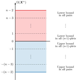
Figure 3: Values of the O-information impose limits on the strength of interactions – as measured by $C(\bm{X}^{\bm{\gamma}})$ – at different scales. Positive (negative) values of $\Omega$ put lower (upper) bounds on subsets of $\bm{X}^{n}$, and higher absolute values of $\Omega$ put bounds on subsystems of smaller sizes.

The next result corresponds to the converse of Corollary 3, and shows how interactions at different scales limit the achievable values of $\Omega$.

Corollary 4.

For a given $\bm{\gamma}\subset\{1,\dots,n\}$ with $|\bm{\gamma}|=m$, the following bounds on $\Omega$ hold:

$$n-m-1+\frac{C(\bm{X}^{\bm{\gamma}})}{\log|\mathcal{X}|}\geq\frac{\Omega(\bm{X}^{n})}{\log|\mathcal{X}|}\geq-(n-2)+\frac{C(\bm{X}^{\bm{\gamma}})}{\log|\mathcal{X}|}.$$

By comparing it with Lemma 3, this result shows that a large $C(\bm{X}^{\bm{\gamma}})$ does not allow $\Omega$ to reach its lower bound. On the other hand, small values of $C(\bm{X}^{\bm{\gamma}})$ decrease the upper bound, forbidding high values of $\Omega$. Additionally, note that fixing the value of only one subset of $m$ variables reduces the range of values of $\Omega$ from $2(n-2)$ to $2(n-2)-(m-1)$. The following example illustates these findings.

Example 4.

Let us consider a system $\bm{X}^{n}$ of binary variables, two of which are related by the marginal distribution

$$p_{X_{1}X_{2}}(x_{1},x_{2})=\frac{(1-\eta)^{1-|x_{1}-x_{2}|}\eta^{|x_{1}-x_{2}|}}{2}~{}.$$

That is, $X_{1}$ and $X_{2}$ are fair coins linked by a binary symmetric channel with crossover probability $\eta$ (cover2012elements, , Sec. 7). Hence, $C(\bm{X}^{2})=I(X_{1};X_{2})=1-H(\eta)$, with $H(\eta)=-\eta\log\eta-(1-\eta)\log(1-\eta)$ being the binary entropy function. By considering $m=2$, Corollary 4 states that

$$n-2-H(\eta)\geq\Omega(\bm{X}^{n})\geq-\big{(}n-3+H(\eta)\big{)}~{},$$

which is illustrated in Figure 4. Moreover, using Eq. (16) one can verify that the upper bound (solid red line) is attained when $X_{2}=X_{3}=\dots=X_{n}$, while the lower bound (solid blue line) is attained when $X_{3},\dots,X_{n-1}$ are independent fair coins and $X_{n}=\sum_{j=1}^{n-1}X_{j}\pmod{2}$ .

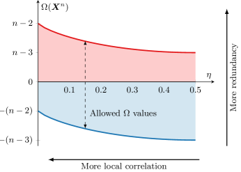
Figure 4: Bounds of the O-information when two variables are connected via a binary symmetric channel with crossover probability $\eta$.

IV.3 $\Omega$ as a superposition of tendencies

This subsection explores sufficient conditions that make a system have a small O-information. As a preliminary step, the next result shows that $\Omega$ is additive for systems with independent subsystems.

Lemma 4.

If $p_{\bm{X}^{n}}(\bm{x}^{n})=\prod_{k=1}^{m}p_{\bm{X}^{\bm{\alpha}_{k}}}(\bm{x}^{\bm{\alpha}_{k}})$ for some partition $\pi=(\bm{\alpha}_{1}|\dots|\bm{\alpha}_{m})$, then

$$\Omega(\bm{X}^{n})=\sum_{k=1}^{m}\Omega(\bm{X}^{\bm{\alpha}_{k}})~{}.$$

Proof.

Let us consider the case $\pi=(\bm{\alpha}_{1},\bm{\alpha}_{2})$, as the general case is then guaranteed by induction. Using Eqs. (14) and (15) it is direct to check that, due to the independence, $C(\bm{X}^{n})=C(\bm{X}^{\bm{\alpha}_{1}})+C(\bm{X}^{\bm{\alpha}_{2}})$ and $B(\bm{X}^{n})=B(\bm{X}^{\bm{\alpha}_{1}})+B(\bm{X}^{\bm{\alpha}_{2}})$. Then, the desired result follows from the fact that $\Omega(\bm{X}^{n})=C(\bm{X}^{n})-B(\bm{X}^{n})$. ∎

Corollary 5.

$\Omega(\bm{X}^{n})=0$ for all systems whose joint distribution can be factorised as

$$p_{\bm{X}^{n}}(\bm{x}^{n})=\prod_{k=1}^{n/2}p_{X_{2k-1}X_{2k}}(x_{2k-1},x_{2k})~{}.$$ (19)

Proof.

Using Eq. (19) and Lemma 4 we find that

$$\Omega(\bm{X}^{n})=\sum_{k=1}^{n/2}\Omega(X_{2k-1},X_{2k})=0\enspace,$$

where the last equality is a consequence of the O-information being zero for sets of two variables, as shown in Proposition 1. ∎

Corollary 5 states that having disjoint pairwise interactions is a sufficient condition for $\Omega=0$ to hold. However, this condition is not necessary: from Lemma 4 we can see that a system composed by redundant ($\Omega>0$) and synergistic ($\Omega<0$) subsystems can attain zero net O-information due to “destructive interference.”

As a consequence, the O-information can be understood as the result of a superposition of behaviours of subsystems. Therefore, $\Omega=0$ can take place in two qualitatively different scenarios: systems in which redundancies and synergies are balanced, or systems with only disjoint pairwise effects. Some of these cases can be resolved by considering the information diagram of $C(\bm{X}^{n})$ and $B(\bm{X}^{n})$ (c.f. Figure 2), or by studying the O-information of parts of the system. However, it is important to remark that redudancy and synergy can coexist either in disjoint subsystems or within the same variables. An insightful example of the latter case can be found in Ref. (james2017multivariate, , Section 2).

As a final remark, note that systems where pairwise interdependencies are overlapping (e.g. pairwise maximum entropy models cofre2018 ) cannot be factorised as required by Corollary 5, and hence can have either positive or negative O-information .

V Relationship with other notions of high-order effects

V.1 High-order interactions in statistical mechanics

A popular approach to address high-order interactions in the statistical physics literature is via Hamiltonians that include interaction terms with three or more variables schneidman2003network . For example, systems of $n$ spins (i.e. $\mathcal{X}_{i}=\{-1,1\}$ for $i=1,\dots,n$) that exhibit $k$-th order interactions are usually represented by probability distributions of the form

$$p_{\bm{X}^{n}}(\bm{x}^{n})=\frac{e^{-\beta\mathcal{H}_{k}(\bm{x}^{n})}}{Z}~{},$$ (20)

where $\beta$ is the inverse temperature, $Z$ is a normalization constant, and $\mathcal{H}(\bm{x}^{n})$ is a Hamiltonian given by

$$\mathcal{H}_{k}(\bm{x}^{n})= -\sum_{i=1}^{n}J_{i}x_{i}-\sum_{i=1}^{n-1}\sum_{j=i+1}^{n}J_{i,j}x_{i}x_{j}$$

$$\dots-\sum_{|\bm{\gamma}|=k}J_{\bm{\gamma}}\prod_{i\in\bm{\gamma}}x_{i}~{},$$

with the last sum runing over all subsets $\bm{\gamma}\subseteq\{1,\dots,n\}$ of size $|\bm{\gamma}|=k$. According to Eq. (20), configurations with lower $\mathcal{H}_{k}(\bm{x}^{n})$ are more likely to be visited. Note that $J_{i}$ quantify external influences acting over individual spins, while $J_{\bm{\gamma}}$ for $|\bm{\gamma}|\geq 2$ represent the strength of the interactions; in particular, if $J_{i,k}>0$ then the pair $X_{i},X_{k}$ tend to be aligned, while if $J_{i,k}<0$ they tend to be anti-aligned. As a matter of fact, $\bm{X}^{n}$ are independent if and only if $J_{\bm{\gamma}}=0$ for all $\bm{\gamma}$ with $|\bm{\gamma}|\geq 2$. Models with $k$-th order interactions have been studied via the maximum entropy principle schneidman2003network , information geometry amari2001information and PID olbrich2015information .

Considering the results presented in previous sections, one could expect that systems with high-order interactions (i.e. large $k$) should attain lower values of $\Omega$ than systems with low-order interactions (i.e. small $k$). To confirm this hypothesis, we studied ensembles of systems with $k$-th order interactions, and analised how the value of $\Omega$ is influenced by $k$. For this, we considered random Hamiltonians with $J_{\bm{\gamma}}$ drawn i.i.d. from a standard normal distribution and $\beta=0.1$.

In agreement with intuition, results show that $\Omega$ is usually very close to zero for $k=2$, and becomes negative as $k$ grows (Figure 5). These results suggest that the notion of synergy measured by $\Omega$ is consistent with the traditional ideas of high-order interactions from statistical physics.

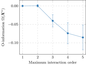
Figure 5: Mean value and confidence intervals of ensembles of systems of $n=5$ spins with randomly generated Hamiltonians. By including high-order interaction terms, net synergy increases and $\Omega$ decreases.

V.2 Complexity and integration

In their seminal 1994 article, Tononi, Edelman, and Sporns devised a measure of complexity (henceforth called TSE complexity) to describe the interplay between local segregation and global integration tononi1994measure ; tononi1998complexity . The TSE complexity is defined as

$$\text{TSE}(\bm{X}^{n})\coloneqq\sum_{k=1}^{n}\left[\frac{k}{n}C(\bm{X}^{n})-C_{n}(k)\right]~{},$$ (21)

where $C_{n}(k)={n\choose k}^{-1}\sum_{|\bm{\gamma}|=k}C(\bm{X}^{\bm{\gamma}})$ is the average total correlation of the subsets $\bm{\gamma}\subseteq\{1,\dots,n\}$ of size $|\bm{\gamma}|=k$. By measuring the convexity of $C_{n}(k)$, the TSE complexity attempts to distinguish scenarios that exhibit “relative statistical independence of small subsets of the system […] and significant deviations from independence of large subsets” (tononi1994measure, , Abstract), in the same spirit as our motivation behind $\Omega$ above.

To study the relationship between the TSE complexity and the O-information, it is useful to consider an alternative expression of the former:

$$\text{TSE}(\bm{X}^{n})=\sum_{k=1}^{\lfloor n/2\rfloor}{n\choose k}^{-1}\sum_{|\bm{\gamma}|=k}I(\bm{X}^{\bm{\gamma}};\bm{X}_{-\bm{\gamma}}^{n})~{},$$ (22)

where $X_{-\bm{\gamma}}^{n}$ represents all the variables that are not in $\bm{\gamma}$, and $\lfloor\cdot\rfloor$ is the floor function. By noting the similarities between Eq. (22) and the sum of $B$ and $C$,

$$C(\bm{X}^{n})+B(\bm{X}^{n})=\sum_{i=1}I(X_{i};\bm{X}_{-i}^{n})~{},$$ (23)

together with the fact that $\text{TSE}(\bm{X}^{3})=\frac{1}{3}\big{[}C(\bm{X}^{3})+B(\bm{X}^{3})\big{]}$, we can hypothesise that, qualitatively,

$$\text{TSE}(\bm{X}^{n})\propto C(\bm{X}^{n})+B(\bm{X}^{n})~{}.$$ (24)

Monte Carlo simulations show that this approximation is justified: when evaluated on distributions $p_{\bm{X}^{n}}$ sampled uniformly at random from the probability simplex, the correlation of Eq. (24) and TSE is consistently above $0.97$ (Figure 6). Moreover, Eq. (24) outperforms other proposed approximations of the TSE complexity .

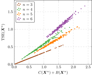
Figure 6: (Color) The sum of the total correlation and the binding entropy is a very accurate approximation of the TSE complexity. Each dot is a probability distribution over $n$ bits sampled uniformly at random from the probability simplex.

Figure 6 and Eq. (24) suggest that the TSE complexity is large when either the shared randomness or the collective constraints are large. As a more direct example, we evaluate TSE in a distribution given by a linear mixture of a 3-bit copy and a 3-bit xor, showing that TSE has exactly the same value in both extremes, and hence that it conflates redundancy with synergy (Figure 7).

Taken together, our results show that the TSE complexity is a good metric of overall integration between parts of the system, but it generally fails to detect synergistic phenomena. Overall, the fact that

$$\begin{split}\Omega&=C-B~{},\\ \text{TSE}&\propto C+B~{},\end{split}$$ (25)

suggests that the TSE complexity and the O-information are complementary, corresponding to an insightful “change of basis” from an elementary constraints vs randomness representation. Effectively, while both $C$ and $B$ provide two measures of roughly the same phenomenon (interdependency strength), $\Omega$ and TSE refer to different aspects: TSE gives an overarching account of the strength of the interdependencies within $\bm{X}^{n}$, and $\Omega$ indicates whether these correlations are predominantly redundant or synergistic.

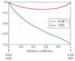
Figure 7: (Color) TSE and $\Omega$ evaluated on a distribution resulting from a linear mixture between a copy (left) and an xor (right), showing that the TSE complexity conflates synergy and redundancy. Figure shows the case $n=3$, but results are qualitatively similar for larger systems

VI Case study: Baroque music scores

To illustrate the proposed framework in a data-driven application, this section presents a study of the multivariate statistics of musical scores from the Baroque period. In the sequel, Section VI.1 describes the procedure to obtain and analyse the data. Results are then presented in Section VI.2. These results are a brief demonstration of the value for the O-information for practical data analysis.

VI.1 Method description

VI.1.1 Data

Our analysis focuses on two sets of repertoire: the well-known chorales for four voices by Johann Sebastian Bach (1685-1750), and the Opus 1 and 3-6 by Arcangelo Corelli (1653-1713). All of these works correspond to the Baroque period (approx. 1600–1750), which is characterised by elaborate counterpoint between melodic lines. Baroque music usually exhibits a balance in the interest and richness of the parts of all the involved instruments, contrasting with the subsequent Classic (1730–1820) and Romantic (1780–1910) periods where higher voices tend to take the lead.

Our analysis is based on the electronic scores publicly available at http://kern.ccarh.org. We focused on scores with four melodic lines: four voices (soprano, alto, tenor and bass) in the case of Bach’s chorales, and four string instruments (1^st violin, 2^nd violin, viola and cello) in the case of Corelli’s pieces. The scores were pre-processed in Python using the Music21 package (http://web.mit.edu/music21), which allowed us to select only the pieces writen in Major mode and to transpose them to C Major. The melodic lines were transformed into time series of 13 possible values (one for each note plus one for the silence), using the smallest rhythmic duration as time unit. This generated $\approx 4\times 10^{4}$ four-note chords for the chorales, and $\approx 8\times 10^{4}$ for Corelli’s pieces. With these data, the joint distribution of the values for the four-note chords was estimated using their empirical frequency .

VI.1.2 Research questions and tools

We focus on the multivariate statistics of the harmonic structures of these pieces. In particular, we ask to what extent the notes played simultaneously by different instruments are redundant or synergistic. Our study focuses exclusively on harmony and chords, leaving melodic properties to future studies.

Let us denote by $\bm{X}^{4}$ the random vector of notes, where $|\mathcal{X}|=13$. We first compute the marginal entropy of each voice, $H(X_{k})$, which is an indicator of harmonic richness. We also compute the O-information of the ensemble $\Omega(\bm{X}^{4})$, which determines the dominant behaviour. Interestingly, for $n=4$ the decomposition in Eq. (16) yields

$$\Omega(\bm{X}^{4})=I(X_{i};X_{j};X_{k},X_{l})+I(X_{k};X_{l};X_{i},X_{j})$$

for $\{i,j,k,l\}=\{1,2,3,4\}$. One can gain a fine-grained view of $\Omega$ by considering these interaction information terms, which can be seen as local contributions to $\Omega$. More formally, we define the local O-information between $X_{i}$ and $X_{j}$ as

$$\omega_{ij}(\bm{X}^{n})\coloneqq I(X_{i};X_{j};\bm{X}^{n}_{-ij})~{},$$ (26)

such that $\Omega$ can be decomposed as a sum of local $\omega$. Interestingly, these local terms could be of the opposite sign to the global $\Omega(\bm{X}^{n})$, indicating local synergy (or redudancy) between two components within a predominantly redundant (or synergistic) system.

Since all the $X_{k}$ take values among alphabets of cardinality $13$, we perform all computations employing logarithms to base $13$, so that $H(X_{k})\leq 1$. We call this unit a mut, for musical bit.

VI.2 Results

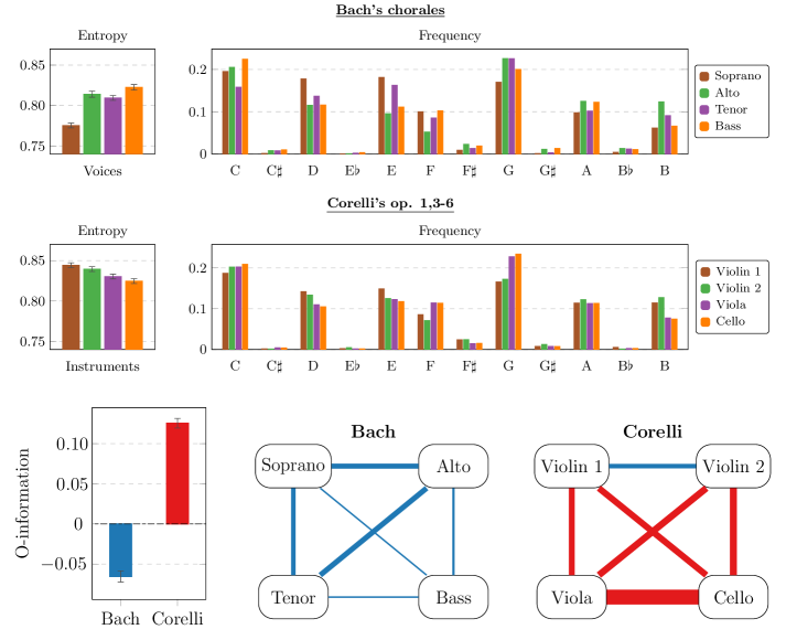
Figure 8: (Color) Above: Entropy of the frequencies of appeareance of each note in the studied pieces of Bach and Corelli, measured in muts (logarithm to base 13); standard errors were estimated via circular block-bootstrap. While the higher voices in Corelli have higher entropy, Bach’s soprano has a lower entropy than all other voices. Below: Global O-information (left), and networks of local O-information (middle, right) with red reflecting redundancy ($w_{ij}>0$) and blue synergy ($w_{ij}<0$). While Bach’s chorales are synergy-dominated, the pieces of Corelli are strongly redundant (mainly due to the viola and cello).

By studying the entropies of each voice, our results confirm that the four voices in these Baroque scores tend to have similar harmonical richness (Figure 8, top left). In fact, their values are similar (although slightly lower) than $\log_{13}7\approx 0.845$ muts, which corresponds to a uniform distibution over the seven notes of a major scale (notes without sharp or flat). Also, our results show that the entropies in the music of Corelli are higher for instruments with higher register (i.e. the violins). In contrast, in Bach’s music the soprano has significantly less entropy than the other voices. This can be explained by the fact that Bach’s pieces were made to be used in public religious services, with the soprano conveying a melodic line that was intended to be sung by the attendees – and hence its structure is simpler to make it easy to sing.

Most strikingly, our analyses of the multivariate structure of the pieces show that Bach’s chorales have negative O-information, suggesting that the harmonic structure of these pieces is dominated by synergistic effects (Figure 8, bottom left). This result is further confirmed by the fact that all the local O-information terms are negative, which means that the pairwise dependence between any pair of voices is comparatively smaller than the global dependencies that exists within the group (see Table 1).

Table 1: Multivariate statistics of Baroque repertoire. For each pair of voices or instruments, we report the mutual information (MI), conditional mutual information (CMI), and local O-information ($\omega_{ij}$). Quantities are measured in musical bits, or muts (logarithm to base 13). Standard errors were estimated via circular block-bootstrap, and in all cases are below the least significant figure shown in the table.

Bach’s chorales
		MI	CMI	$\omega_{ij}$
Soprano	Alto	0.14	0.19	-0.05
Soprano	Tenor	0.12	0.16	-0.04
Soprano	Bass	0.15	0.16	-0.02
Alto	Tenor	0.17	0.22	-0.05
Alto	Bass	0.15	0.17	-0.02
Tenor	Bass	0.15	0.17	-0.02
Corelli’s op. 1,3-6
		MI	CMI	$\omega_{ij}$
Violin 1	Violin 2	0.071	0.115	-0.04-
Violin 1	Viola	0.086	0.028	0.06
Violin 1	Cello	0.095	0.034	0.06
Violin 2	Viola	0.118	0.054	0.07
Violin 2	Cello	0.107	0.039	0.07
Viola	Cello	0.630	0.460	0.17

In contrast, Corelli’s pieces have positive O-information, suggesting that they are dominated by a redundant component. Interestingly, the local O-information has a positive value for all pairs except for violins 1 and 2. The strongest O-information is the one between viola and cello, indicating that the parts of these two instruments are highly redundant.

The redundancy in the pieces of Corelli can be explained by compositional practices for intrumental music in the Baroque period. In fact, the original score of many of the studied pieces was written for only three parts: two solists and a bass line called “basso continuo.” This bass line was suposed to be interpreted in different ways by the bass instruments, which in this case correspond to viola and cello. Therefore, it is fair to say that these instruments are redundant, as both of them are carrying the same bass line. Despite this redundancy, the relationship between the violins is still synergistic, which is appropiately captured by the negative value of their local O-information.

The dominance of synergy in the case of Bach can be argued to serve an artistic purpose – in effect, in the Baroque period the aim was that each voice should introduce unique elements into the piece. This goal could be achieved by superposing unrelated melodies; however, the overall result might not have been aesthetically pleasing due to the lack of global coordination. A synergistic structure serves this purpose well, as it provides global constraints that ensure collective coherence while imposing weak pairwise constraints.

VII Conclusion

We introduced $\Omega(\bm{X}^{n})$ as the difference between strength of the collective constraints and the shared randomness in a multivariate system $\bm{X}^{n}$. We argued that $\Omega$ captures the net balance between statistical synergy and redundancy, since (i) it is a sum of triple interaction informations, (ii) it is maximised (minimised) by an $n$-bit copy (xor), and (iii) it imposes bounds over the intedependency allowed at different scales. According to this framework, synergistic systems are characterised by a large amount of shared randomness regulated by weak collective constraints, which is consistent with recent approaches to study emergence based on constructive logic pascual2018constructive . Moreover, in deriving $\Omega$, we also provided a joint source of explanation for three long-standing extensions of Shannon’s mutual information (total correlation, binding entropy, and interaction information) in terms of shared randomness and collective constraints. The proposed framework is straightforward to generalise to continuous variables and apply to neural data, which will be presented in a separate publication.

The O-information was compared to other notions of high-order effects, most notably the TSE complexity tononi1994measure . We found that TSE does not measure statistical synergy as such, but total correlation strength. Moreover, our analysis suggest that $\Omega$ and TSE are complementary metrics: TSE gives an overarching account of the strength of the interdependencies within $\bm{X}^{n}$, and the O-information reveals whether these correlations are predominantly redundant or synergistic. We take this as a step towards a multi-dimensional framework that allows for a finer and more subtle taxonomy of complex systems.

Finally, we applied our framework to Baroque music scores and found that Bach’s chorales, unlike pieces by some of his contemporaries, are strongly synergistic as measured by $\Omega$. Informally, we can speculate about the artistic role of synergy: synergistic music (like Bach’s) allows each voice to contribute unique material while ensuring an overall harmonious integration of the ensemble. This delicate balance has an intriguing similarity with the coexistence of integration and differentiation in brain activity tononi1998complexity ; balduzzi2008integrated , suggesting unexplored relationships between music structure and neural organisation.

Appendix A Compatibility between $\Omega$ and prior work

In prior work rosas2018selforg , we introduced $\psi(k)$ as

$$\psi(k)\coloneqq\max_{j\in\{1,\dots,n\}}\max_{\begin{subarray}{c}\bm{\gamma}\subseteq\{1,\dots,n\}\\ |\bm{\gamma}|=k,j\notin\bm{\gamma}\end{subarray}}I(X_{j};\bm{X}^{\bm{\gamma}})~{}.$$

The growth profile of this non-decreasing function was taken as an indicator of the leading quality of the interdependency structure of $\bm{X}^{n}$, being convexity associated with statistical synergy, and concavity with redundancy  (rosas2018selforg, , Definition 2).

The relationship between these ideas and the ones developed in this article can be established by noting that convexity in $\psi(k)$ implies that small scales of the system are relatively independent while large scales show correlation, which – due to the results of Section IV.2 – is the key characteristic of synergy-dominated systems. Conversely, concavity in $\psi(k)$ implies that some small groups of variables are highly correlated, which implies a relatively high value of $C(\bm{X}^{n})$ and $\Omega(\bm{X}^{n})$.

To enable a quantitative comparison between $\psi(k)$ and $\Omega$, one can quantify the convexity/concavity of the former by measuring the distance from $\psi(k)$ to a straight line joining $\psi(1)$ and $\psi(n)$ as

$$\Psi(\bm{X}^{n})\coloneqq\sum_{k=1}^{n}\left[\psi(k)-\left(\frac{k}{n}\big{[}\psi(n)-\psi(1)\big{]}+\psi(1)\right)\right]~{}.$$

We computed $\Omega$ and $\Psi$ of binary systems of different sizes generated randomly from a uniform distribution over the corresponding probability simplex. Our results show a good agreement between these two metrics, which confirms the analytic reasoning presented above.

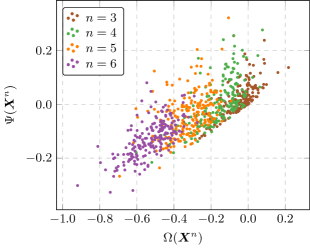
Figure 9: The O-information and $\Psi$ – introduced in our previous work rosas2018selforg – have good agreement.

In summary, $\Omega$ can be regarded as a formalisation of the intuitive notions introduced in rosas2018selforg . Moreover, $\Omega$ possesses more theoretical properties than $\Psi$ and requires the calculation of a smaller number of terms.

Appendix B $R(\pi)$ decreases for finer partitions

Lemma 5.

Let us consider two partitions $\pi_{\text{a}}=(\bm{\alpha}_{1}|\dots|\bm{\alpha}_{K})$ and $\pi_{\text{b}}=(\bm{\beta}_{1}|\dots|\bm{\beta}_{J})$ such that $\pi_{\text{b}}\succeq\pi_{\text{a}}$. Then, $R(\pi_{\text{b}})\leq R(\pi_{\text{a}})$.

Proof.

Let us assume that $\pi_{\text{a}}=(\bm{\alpha}_{1}|\dots|\bm{\alpha}_{K}\}$, $\pi_{\text{b}}=(\bm{\beta}_{1}|\dots|\bm{\beta}_{J})$ such that $\pi_{\text{b}}\succeq\pi_{\text{a}}$, and consider a path $\texttt{p}=(\pi_{1},\dots,\pi_{L})$ in $\texttt{P}(\pi_{\text{a}},\pi_{\text{b}})$ so that $\pi_{1}=\pi_{\text{a}}$ and $\pi_{L}=\pi_{\text{b}}$. To prove the Lemma suffices to show that $R(\pi_{j+1})\leq R(\pi_{j})$ for $j=1,\dots,L-1$. As $\pi_{1},\dots,\pi_{n}$ are related by covering relationships, one just needs to prove the inequality for two partitions such that one covers the other.

Consider $\pi_{1},\pi_{2}\in\mathcal{P}_{n}$ such that $\pi_{2}$ covers $\pi_{1}$. As both partitions differ only in one elementary refinement, let us without loss of generality assume that the refinement is done on the last cell of $\pi_{1}$; i.e. $\pi_{1}=(\bm{\alpha}_{1}|\dots|\bm{\alpha}_{m})$ and $\pi_{2}=(\bm{\alpha}_{1}|\dots|\bm{\alpha}_{m-1}|\tilde{\bm{\alpha}}_{m}|\tilde{\bm{\alpha}}_{m+1})$ so that $\tilde{\bm{\alpha}}_{m}\cup\tilde{\bm{\alpha}}_{m+1}=\bm{\alpha}_{m}$ and $\tilde{\bm{\alpha}}_{m}\cap\tilde{\bm{\alpha}}_{m+1}=\varnothing$. Then

$$R(\pi_{1})-R(\pi_{2}) =R_{\bm{\alpha}_{m}}-(R_{\tilde{\bm{\alpha}}_{m}}+R_{\tilde{\bm{\alpha}}_{m+1}})$$

$$=I(\bm{X}^{\tilde{\bm{\alpha}}_{m}};\bm{X}^{\tilde{\bm{\alpha}}_{m+1}}|\bm{X}^{\bm{\alpha}_{1}}\dots\bm{X}^{\bm{\alpha}_{m-1}})$$

$$\geq 0\enspace,$$

proving the desired result. ∎

Appendix C Proof of Lemma 2

Proof.

Consider a path $\mathtt{p}\in\texttt{P}(\pi_{\text{source}},\pi_{\text{sink}})$, so that $\texttt{p}=(\pi_{1},\dots,\pi_{L})$ with $\pi_{1}=\pi_{\text{source}}$ and $\pi_{L}=\pi_{\text{sink}}$. Then, by using Eqs. (8) and (9), a direct calculation shows that

$$W(\texttt{p};v_{h}) =\sum_{j=1}^{L-1}\big{[}H(\pi_{j+1})-H(\pi_{j})\big{]}$$

$$=H(\pi_{\text{sink}})-H(\pi_{\text{source}})$$

$$=\sum_{i=1}^{n}H(X_{i})-H(\bm{X}^{n})~{}.$$

Similarly, using Eqs. (8) and (10) gives

$$W(\texttt{p};v_{\text{r}})= \sum_{j=1}^{L-1}\left[R(\pi_{j})-R(\pi_{j+1})\right]$$

$$= R(\pi_{\text{source}})-R(\pi_{\text{sink}})$$

$$= H(\bm{X}^{n})-\sum_{i=1}^{n}H(X_{i}|\bm{X}^{n}_{-i})~{}.$$

Both results make use of the fact that $W(\texttt{p};v_{\text{h}})$ and $W(\texttt{p};v_{\text{r}})$ are telescopic sums and all but the first and last terms cancel out. ∎

Appendix D Proof of Proposition 1

Proof.

Let us consider a path $\mathtt{p}\in\texttt{P}(\pi_{\text{source}},\pi_{\text{sink}})$. Then,

$$W(\mathtt{p};v_{\text{s}}) =\sum_{j=1}^{L}v_{\text{s}}(\pi_{j},\pi_{j+1})$$ (27)

$$=\sum_{j=1}^{L}v_{\text{h}}(\pi_{j},\pi_{j+1})-\sum_{k=1}^{L}v_{\text{r}}(\pi_{k},\pi_{k+1})$$

$$=C(\bm{X}^{n})-B(\bm{X}^{n})=\Omega(\bm{X}^{n}),$$

which proves the first part of the theorem.

Thanks to Eq. (27), one can prove the second part of the Theorem by showing that if $\pi_{\text{a}},\pi_{\text{b}}\in\mathcal{P}_{n}$ such that $\pi_{\text{b}}\succeq\pi_{\text{a}}$, then $v_{\text{s}}(\pi_{1},\pi_{2})$ is equal to an interaction information. To show this, first note that if $\pi_{\text{b}}\succeq\pi_{\text{a}}$ then both partitions differ only in one elementary refinement. Without no loss of generality, we assume that the refinement is done on the last cell, such that $\pi_{\text{a}}=(\bm{\alpha}_{1}|\dots|\bm{\alpha}_{m})$ and $\pi_{\text{b}}=(\bm{\alpha}_{1}|\dots|\bm{\alpha}_{m-1}|\tilde{\bm{\alpha}}_{m}|\tilde{\bm{\alpha}}_{m+1})$ such that $\tilde{\bm{\alpha}}_{m}\cap\tilde{\bm{\alpha}}_{m+1}=\varnothing$ and $\tilde{\bm{\alpha}}_{m}\cup\tilde{\bm{\alpha}}_{m+1}=\bm{\alpha}_{m}$. Then,

$$v_{\text{s}}(\pi_{\text{a}},\pi_{\text{b}}) =v_{\text{h}}(\pi_{\text{a}},\pi_{\text{b}})-v_{\text{r}}(\pi_{\text{a}},\pi_{\text{b}})$$

$$=\big{[}H(\pi_{\text{b}})-H(\pi_{\text{a}})\big{]}-\big{[}R(\pi_{\text{a}})-R(\pi_{\text{b}})\big{]}$$

$$=I(\bm{X}^{\tilde{\bm{\alpha}}_{m}};\bm{X}^{\tilde{\bm{\alpha}}_{m+1}})$$

$$\quad-I(\bm{X}^{\tilde{\bm{\alpha}}_{m}};\bm{X}^{\tilde{\bm{\alpha}}_{m+1}}|\bm{X}^{\bm{\alpha}_{1}}\dots\bm{X}^{\bm{\alpha}_{m-1}})$$

$$=I(\bm{X}^{\tilde{\bm{\alpha}}_{m}};\bm{X}^{\tilde{\bm{\alpha}}_{m+1}};\bm{X}^{\bm{\alpha}_{1}}\dots\bm{X}^{\bm{\alpha}_{m-1}})\enspace,$$

which proves the desired result. ∎

Appendix E Proof of Lemma 3

Proof.

Let us first note that

$$\log|\mathcal{X}| \geq I(X_{i};X_{j}|X_{k})\geq 0\enspace,$$ (28)

$$\log|\mathcal{X}| \geq I(X_{i};X_{j};X_{k})\geq-\log|\mathcal{X}|\enspace,$$ (29)

for all $i,j,k\in\{1,\dots,n\}$. Above, Eq. (29) follows from noting that $I(X_{i};X_{j};X_{k})=I(X_{i};X_{j})-I(X_{i};X_{j}|X_{k})$, and applying the bounds in Eq. (28). The proposition is proved by applying these inequalities on Eqs. (14), (15), (16), and (23). Finally, the tightness of the bounds is a direct consequence of the tightness of Eqs. (28) and (29). ∎

Appendix F Proof of Proposition 2

Proof.

Let us first prove the first statement. By considering $\bm{X}^{n}$ to be a $n$-bit copy, a direct calculation using Eqs. (14) and (15) shows that $C(\bm{X}^{n})=n-1$ and $B(\bm{X}^{n})=1$, and therefore the upper bound is attained. To prove the converse, let us start by assuming that $\Omega(\bm{X}^{n})=n-2$. By applying (29) to each term in (16), is clear that $I(X_{j};\bm{X}^{j-1};\bm{X}_{j+1}^{n})=1$ holds for all $j\in\{1,\dots,n\}$. In particular $I(X_{2};X_{1};\bm{X}_{3}^{n})=1$ holds, which due to Eq. (16) implies that $I(X_{2};X_{1}|\bm{X}_{3}^{n})=0$ and hence $I(X_{2};X_{1})=1$, which in turns implies that $X_{1}$ and $X_{2}$ are Bernoulli distributed with parameter $p=1/2$, and also that $X_{1}=X_{2}$. By relabelling the variables and following the same rationale one can prove that every pair of variables are equal to each other, which proves that $\bm{X}^{n}$ is a $n$-bit copy.

Let us prove the second statement. By considering now $\bm{X}^{n}$ to be a $n$-bit xor, using Eqs. (14) and (15) it is direct to check that $C(\bm{X}^{n})=1$ and $B(\bm{X}^{n})=n-1$, and hence the lower bound is attained. To prove the converse, let us assume that $\bm{X}^{n}$ is such that $\Omega(\bm{X}^{n})=2-n$. By considering the bounds given by Eq. (29) in Eq. (16), this implies that $I(X_{j};\bm{X}^{j-1};\bm{X}_{j+1}^{n})=-1$ for all $j\in\{2,\dots,n-1\}$, and in particular $I(\bm{X}^{n-2};X_{n-1};X_{n})=-1$. Due to Eq. (29), this implies in turn that $I(\bm{X}^{n-2};X_{n-1})=0$, and via relabeling one can prove that $\bm{X}^{n-1}$ are jointly independent. Moreover, $I(\bm{X}^{n-2};X_{n-1};X_{n})=-1$ also implies that $I(X_{n-1};X_{n}|\bm{X}^{n-2})=1$, which implies that

$$I(\bm{X}^{n-1};X_{n})=I(X_{n-1};X_{n}|\bm{X}^{n-2})+I(\bm{X}^{n-2};X_{n})=1.$$

This equality implies that $X_{n}$ is Bernoulli distributed with $p=1/2$, and that $X_{n}$ is a deterministic function of $\bm{X}^{n-1}$. Moreover, the fact that $I(X_{1};X_{n}|\bm{X}_{2}^{n-1})=1$ implies that for given $\bm{X}_{2}^{n-1}$ then $X_{n}$ is a function of $X_{1}$, while via relabelling one finds that $I(X_{1};X_{n})=0$. Since the only functions with these properties are functions isomorphic to an $n$-variate xor, this proves the desired result. ∎

Appendix G Proof of Proposition 3

The following proof uses Lemma 6, which is stated and proved afterwards in this Appendix.

Proof.

To prove Eq. (17), first note that

$$\Omega(\bm{X}^{n})=C(\bm{X}^{n-1})-B(\bm{X}^{n-1}|X_{n})\leq C(\bm{X}^{n-1})~{}.$$

Then, the inequality follows form a direct application of Lemma 6. As $C(\bm{X}^{m})\geq 0$, the equality becomes non-trivial when

$$\Omega(\bm{X}^{n})-(n-m-1)\log|\mathcal{X}|\geq 0\enspace.$$

To prove Eq. (18), note that by using Eqs. (14), (15), and (16) one can find that

$$\Omega(\bm{X}^{n})= C(\bm{X}^{m})-B(\bm{X}^{m}|\bm{X}_{m+1}^{n})$$

$$+\sum_{j=m+1}^{n-1}I(X_{j};\bm{X}^{j-1};\bm{X}_{j+1}^{n})$$

$$\geq C(\bm{X}^{m})-(n-2)\log|\mathcal{X}|.$$

Above, the inequality is due to $I(X_{j};\bm{X}^{j-1};\bm{X}_{j+1}^{n})\leq\log|\mathcal{X}|$ and $B(\bm{X}^{m}|\bm{X}_{m+1}^{n})\leq(m-1)\log|\mathcal{X}|$. As the above relationship does not depend on the labelling of the $X$’s, this proves Eq. (18). As $C(\bm{X}^{m})\leq(m-1)\log|\mathcal{X}|$, the equality becomes non-trivial when

$$\Omega(\bm{X}^{n})+(n-2)\log|\mathcal{X}|\leq(m-1)\log|\mathcal{X}|\enspace.$$

∎

Lemma 6.

If $|\mathcal{X}|=\min_{i=1,\dots,n}|\mathcal{X}_{i}|$, then

$$\min_{|\bm{\gamma}|=m}C(\bm{X}^{\gamma})\geq C(\bm{X}^{n})-(n-m)\log|\mathcal{X}|~{}.$$

Proof.

A direct calculation using Eq. (14) shows that

$$C(\bm{X}^{n}) =C(\bm{X}^{m})+\sum_{j=m+1}^{n}I(X_{j};\bm{X}^{j-1})$$

$$\leq C(\bm{X}^{m})+(n-m)\log|\mathcal{X}|.$$

As the labelling of the indices can be modified without changing this result, this suffices to prove the desired result. ∎

References

- (1) J. P. Crutchfield, “The calculi of emergence,” Physica D, vol. 75, no. 1-3, pp. 11–54, 1994.
- (2) E. Schneidman, W. Bialek, and M. J. Berry, “Synergy, redundancy, and independence in population codes,” Journal of Neuroscience, vol. 23, no. 37, pp. 11 539–11 553, 2003.
- (3) P. E. Latham and S. Nirenberg, “Synergy, redundancy, and independence in population codes, revisited,” Journal of Neuroscience, vol. 25, no. 21, pp. 5195–5206, 2005.
- (4) E. Ganmor, R. Segev, and E. Schneidman, “Sparse low-order interaction network underlies a highly correlated and learnable neural population code,” Proceedings of the National Academy of Sciences, vol. 108, no. 23, pp. 9679–9684, 2011.
- (5) G. Tononi, G. M. Edelman, and O. Sporns, “Complexity and coherency: integrating information in the brain,” Trends in Cognitive Sciences, vol. 2, no. 12, pp. 474 – 484, 1998.
- (6) D. Balduzzi and G. Tononi, “Integrated information in discrete dynamical systems: motivation and theoretical framework,” PLoS Computational Biology, vol. 4, no. 6, p. e1000091, 2008.
- (7) I. Gat and N. Tishby, “Synergy and redundancy among brain cells of behaving monkeys,” in Advances in Neural Information Processing Systems, 1999, pp. 111–117.
- (8) G. Chechik, A. Globerson, M. J. Anderson, E. D. Young, I. Nelken, and N. Tishby, “Group redundancy measures reveal redundancy reduction in the auditory pathway,” in Advances in Neural Information Processing Systems, 2002, pp. 173–180.
- (9) V. Varadan, D. M. Miller III, and D. Anastassiou, “Computational inference of the molecular logic for synaptic connectivity in C. elegans,” Bioinformatics, vol. 22, no. 14, pp. e497–e506, 2006.
- (10) E. Schneidman, S. Still, M. J. Berry, and W. Bialek, “Network information and connected correlations,” Physical Review Letters, vol. 91, no. 23, p. 238701, 2003.
- (11) G. Tononi, O. Sporns, and G. Edelman, “A measure for brain complexity: relating functional segregation and integration in the nervous system,” Proceedings of the National Academy of Sciences, vol. 91, no. 11, pp. 5033–5037, 1994.
- (12) A. B. Barrett and A. K. Seth, “Practical measures of integrated information for time-series data,” PLoS Computational Biology, vol. 7, no. 1, p. e1001052, 2011.
- (13) P. A. M. Mediano, A. K. Seth, and A. B. Barrett, “Measuring integrated information: Comparison of candidate measures in theory and simulation,” Entropy, vol. 21, no. 1, 2018.
- (14) An exception is the connected information, which can be elegantly derived from principles of information geometry amari2001information ; however, there are no known methods to compute this metric from data.
- (15) P. L. Williams and R. D. Beer, “Nonnegative decomposition of multivariate information,” arXiv preprint arXiv:1004.2515, 2010.
- (16) V. Griffith and C. Koch, “Quantifying synergistic mutual information,” in Guided Self-Organization: Inception. Springer, 2014, pp. 159–190.
- (17) M. Wibral, V. Priesemann, J. W. Kay, J. T. Lizier, and W. A. Phillips, “Partial information decomposition as a unified approach to the specification of neural goal functions,” Brain and Cognition, vol. 112, pp. 25–38, 2017.
- (18) A. B. Barrett, “Exploration of synergistic and redundant information sharing in static and dynamical gaussian systems,” Physical Review E, vol. 91, p. 052802, May 2015.
- (19) R. A. Ince, “Measuring multivariate redundant information with pointwise common change in surprisal,” Entropy, vol. 19, no. 7, p. 318, 2017.
- (20) R. James, J. Emenheiser, and J. Crutchfield, “Unique information via dependency constraints,” Journal of Physics A: Mathematical and Theoretical, 2018.
- (21) C. Finn and J. T. Lizier, “Pointwise partial information decomposition using the specificity and ambiguity lattices,” Entropy, vol. 20, no. 4, p. 297, 2018.
- (22) T. M. Tax, P. A. M. Mediano, and M. Shanahan, “The partial information decomposition of generative neural network models,” Entropy, vol. 19, no. 9, 2017.
- (23) M. Wibral, C. Finn, P. Wollstadt, J. T. Lizier, and V. Priesemann, “Quantifying information modification in developing neural networks via partial information decomposition,” Entropy, vol. 19, no. 9, 2017.
- (24) A. El Gamal and Y.-H. Kim, Network Information Theory. Cambridge university press, 2011.
- (25) S. Watanabe, “Information theoretical analysis of multivariate correlation,” IBM Journal of Research and Development, vol. 4, no. 1, pp. 66–82, 1960.
- (26) T. S. Han, “Linear dependence structure of the entropy space,” Information and Control, vol. 29, no. 4, pp. 337–368, 1975.
- (27) R. G. James, C. J. Ellison, and J. P. Crutchfield, “Anatomy of a bit: Information in a time series observation,” Chaos: An Interdisciplinary Journal of Nonlinear Science, vol. 21, no. 3, p. 037109, 2011.
- (28) V. S. Vijayaraghavan, R. G. James, and J. P. Crutchfield, “Anatomy of a spin: the information-theoretic structure of classical spin systems,” Entropy, vol. 19, no. 5, p. 214, 2017.
- (29) W. J. McGill, “Multivariate information transmission,” Psychometrika, vol. 19, no. 2, pp. 97–116, 1954.
- (30) H. K. Ting, “On the amount of information,” Theory of Probability and its Applications, pp. 439–447, 1962.
- (31) R. W. Yeung, “A new outlook on shannon’s information measures,” Information Theory, IEEE Transactions on, vol. 37, no. 3, pp. 466–474, 1991.
- (32) This disctinction might not have been stressed in the past because most studies focus on bivariate interactions between two sets of variables, for which these two effects are equivalent and equal to the mutual information. However, for interactions involving three or more variables these perspectives differ.
- (33) E. T. Jaynes, Probability Theory: The Logic of Science. Cambridge university press, 2003.
- (34) T. M. Cover and J. A. Thomas, Elements of Information Theory. John Wiley & Sons, 2012.
- (35) For a quantum-mechanical treatment of this notion, see (breuer2002theory, , Ch. 2).
- (36) L. Brillouin, “The negentropy principle of information,” Journal of Applied Physics, vol. 24, no. 9, pp. 1152–1163, 1953.
- (37) This observation can be made rigorous via the Shannon-McMillan-Breiman theorem (cover2012elements, , Sec. 3).
- (38) M. Studenỳ and J. Vejnarová, “The multiinformation function as a tool for measuring stochastic dependence,” in Learning in Graphical Models. Springer, 1998, pp. 261–297.
- (39) In fact, a direct calculation shows that the variables are independent if and only if .
- (40) S. A. Abdallah and M. D. Plumbley, “A measure of statistical complexity based on predictive information with application to finite spin systems,” Physics Letters A, vol. 376, no. 4, pp. 275–281, 2012.
- (41) S. Verdú and T. Weissman, “Erasure entropy,” in Information Theory, IEEE International Symposium on. IEEE, 2006, pp. 98–102.
- (42) ——, “The information lost in erasures,” Information Theory, IEEE Transactions on, vol. 54, no. 11, pp. 5030–5058, 2008.
- (43) E. Olbrich, N. Bertschinger, N. Ay, and J. Jost, “How should complexity scale with system size?” The European Physical Journal B, vol. 63, no. 3, pp. 407–415, 2008.
- (44) The interaction information is closely related to the I-measures yeung1991 , the co-information Bell2003 , and the multi-scale complexity bar2004multiscale .
- (45) F. Rosas, V. Ntranos, C. J. Ellison, S. Pollin, and M. Verhelst, “Understanding interdependency through complex information sharing,” Entropy, vol. 18, no. 2, p. 38, 2016.
- (46) F. Rosas, P. A. Mediano, M. Ugarte, and H. J. Jensen, “An information-theoretic approach to self-organisation: Emergence of complex interdependencies in coupled dynamical systems,” Entropy, vol. 20, no. 10, 2018.
- (47) A lattice is a partially ordered set with a unique infimum and supremum. For more details on this construction, see stanley2012 .
- (48) If with and , is finer than if for each exists such that .
- (49) It is direct to see that covers if and only if it is an “elementary refinement”, i.e. can be obtained from by dividing one cell of in two. Hence, if covers then , where is the number of (non-empty) cells of .
- (50) Put simply, there is an edge from to if results from taking and splitting one of its cells in two.
- (51) It is direct to check that if and only if . Moreover, all have the same length, given by , where is the number of edges in the path.
- (52) In effect, represents the portion of the entropy of the -th cell that is not shared with other cells.
-
(53)
The number of the nodes of grows with the Bell numbers, known for their super-exponential growth rate comtet2012advanced . To find the number of paths in , note that if
one starts from the sink and moves towards the source, every step corresponds
to merging two cells into one. Therefore, as selecting two out of cells
gives choices, the total number
of paths is given by
which grows faster than the Bell numbers. - (54) Interestingly, despite the correlation between and , an -bit xor still enables the most synergistic configuration attainable.
- (55) R. G. James and J. P. Crutchfield, “Multivariate dependence beyond shannon information,” Entropy, vol. 19, no. 10, p. 531, 2017.
- (56) R. Cofré, C. Maldonado, and F. Rosas, “Large deviations properties of maximum entropy markov chains from spike trains,” Entropy, vol. 20, no. 8, 2018.
- (57) For a detailed discussion of this issue for the case of three variables see (rosas2016understanding, , Sec. 5).
- (58) S.-I. Amari, “Information geometry on hierarchy of probability distributions,” Information Theory, IEEE Transactions on, vol. 47, no. 5, pp. 1701–1711, 2001.
- (59) E. Olbrich, N. Bertschinger, and J. Rauh, “Information decomposition and synergy,” Entropy, vol. 17, no. 5, pp. 3501–3517, 2015.
- (60) In (tononi1998complexity, , Fig. 2) the binding entropy (under the name “interaction complexity”) is proposed as a metric “related but not identical to neural complexity.” Numerical evaluations show that the combination of total correlation and binding entropy, as proposed in (24), is a more accurate approximation for the TSE complexity (results not shown).
- (61) Regularisation methods (such as Laplace smoothing) were found to have strong effects the results. We decided not to use such methods, as some chords (e.g. C-C-D-D) are just not going to take place in the Baroque repertoire.
- (62) A. Pascual-Garcia, “A constructive approach to the epistemological problem of emergence in complex systems,” PLoS ONE, vol. 13, no. 10, p. e0206489, 2018.
- (63) H.-P. Breuer and F. Petruccione, The Theory of Open Quantum Systems. Oxford University Press, 2002.
- (64) A. J. Bell, “The co-information lattice,” in Proceedings of the Fifth International Workshop on Independent Component Analysis and Blind Signal Separation, 2003.
- (65) Y. Bar-Yam, “Multiscale complexity/entropy,” Advances in Complex Systems, vol. 7, no. 01, pp. 47–63, 2004.
- (66) R. P. Stanley, Enumerative Combinatorics, ser. Cambridge Studies in Advanced Mathematics. Cambridge University Press;, 2012, vol. Vol. 1.
- (67) L. Comtet, Advanced Combinatorics: The Art of Finite and Infinite Expansions. Springer Science & Business Media, 2012.