english
A numerical scheme for the quantile hedging problem
Abstract
We consider the numerical approximation of the quantile hedging price in a non-linear market. In a Markovian framework, we propose a numerical method based on a Piecewise Constant Policy Timestepping (PCPT) scheme coupled with a monotone finite difference approximation. We prove the convergence of our algorithm combining BSDE arguments with the Barles & Jakobsen and Barles & Souganidis approaches for non-linear equations. In a numerical section, we illustrate the efficiency of our scheme by considering a financial example in a market with imperfections.
Key words: Quantile hedging, BSDEs, monotone approximation schemes
1 Introduction
In this work, we study the numerical approximation of the quantile hedging price of a European contingent claim in a market with possibly some imperfections. The quantile hedging problem is a specific case of a broader class of approximate hedging problems. It consists in finding the minimal initial endowment of a portfolio that will allow the hedging a European claim with a given probability of success, the case corresponding to the classical problem of (super)replication. This approach has been made popular by the work of Föllmer and Leukert [19] who provided a closed form solution in a special setting.
The first PDE characterisation was introduced by [8] in a possibly incomplete market setting with portfolio constraints. Various extensions have been considered since this work: to jump dynamics [25]; to the Bermudan case [6] and American case [16]; to a non-Markovian setting [7, 15]; and to a finite number of quantile constraints [9].
Except for [6, 9], all the aforementioned works are of a theoretical nature. The lack of established numerical methods for these problems is a clear motivation for our study. We now present in more detail the quantile hedging problem and the new numerical method we introduce and study in this paper.
On a complete probability space , we consider a -dimensional Brownian motion and denote by its natural filtration. We suppose that all the randomness comes from the Brownian motion and assume that .
Let , , where is the set of matrices with real entries, be Lipschitz continuous functions, with Lipschitz constant .
For and , which denotes the set of predictable square-integrable processes, we consider the solution to the following stochastic differential equations:
In the financial applications we are considering, will typically represent the log-price of risky assets, the control process is the amount invested in the risky assets, and the function is non-linear to allow to take into account some market imperfections in the model. A typical financial example, which will be investigated in the numerical section, is the following:
Example 1.1.
The underlying diffusion is a one-dimensional Brownian motion with constant drift and volatility . There is a constant borrowing rate and a lending rate with . In this situation, the function is given by:
The quantile hedging problem corresponds to the following stochastic control problem: for find
| (1.1) |
The main objective of this paper is to design a numerical procedure to approximate the function by discretizing an associated non-linear PDE first derived in [8]. A key point in the derivation of this PDE is to observe that the above problem can be reformulated as a classical stochastic target problem by introducing a new control process representing the conditional probability of success. To this end, for , we denote
and by the set of such that . The problem (1.1) can be rewritten as
(see Proposition 3.1 in [8] for details). In our framework, the above singular stochastic control problem admits a representation in terms of a non-linear expectation, generated by a Backward Stochastic Differential Equation (BSDE),
| (1.2) |
where is the solution to
The article [7] justifies the previous representation and proves a dynamic programming principle for the control problem in a general setting. In the Markovian setting, this would lead naturally to the following PDE for in :
| (1.3) |
where for , and , , denoting , we define
| (1.4) |
with
| (1.5) | ||||
| (1.6) |
The PDE formulation in (1.3) is not entirely correct as the supremum part may degenerate and it would require using semi-limit relaxation to be mathematically rigourous. We refer to [8], where it has been obtain in a more general context. We shall use an alternative PDE formulation to this “natural” one (1.3), which we give at the start of Section 2.
Moreover, the value function continuously satisfies the following boundary conditions in the -variable:
| (1.7) |
where is the super-replication price of the contingent claim with payoff .
It is also known that has a discontinuity as . By definition, the terminal condition is
but the values which are continuously attained are obtained by convexification [8], namely
| (1.8) |
and we shall work with this terminal condition at from now on.
To design the numerical scheme to approximate , we use the following strategy:
-
1.
Bound and discretise the set where the controls take their values.
-
2.
Consider an associated Piecewise Constant Policy Timestepping (PCPT) scheme for the control processes .
-
3.
Use a monotone finite difference scheme to approximate in time and space the PCPT solution resulting from 1. & 2.
The approximation of controlled diffusion processes by ones where policies are piecewise constant in time was first analysed by [23]; in [24], this procedure is used in conjunction with Markov chain approximations to diffusion processes to construct fully discrete approximation schemes to the associated Bellman equations and to derive their convergence order. An improvement to the order of convergence from [23] was shown recently in [22] using a refinement of Krylov’s original, probabilistic techniques.
Using purely viscosity solution arguments for PDEs, error bounds for such approximations are derived in [3], which are weaker than those in [23] for the control approximation scheme, but improve the bounds in [24] for the fully discrete scheme. In [27], using a switching system approximation introduced in [3], convergence is proven for a generalised scheme where linear PDEs are solved piecewise in time on different meshes, and the control optimisation is carried out at the end of time intervals using possibly non-monotone, higher order interpolations. An extension of the analysis in [27] to jump-processes and non-linear expectations is given in [17].
Our first contribution is to prove that the approximations built in step 1. and 2. above are convergent for the quantile hedging problem, which has substantial new difficulties compared to the settings considered in the aforementioned works. For this we rely heavily on the comparison theorem for the formulation in (2.1) and we take advantage of the monotonicity property of the approximating sequences. The main new difficulties come from the non-linear form of the PDE including unbounded controls, and in particular the boundaries in the -variable. To deal with the latter especially, we rely on some fine estimates for BSDEs to prove the consistency of the scheme including the strong boundary conditions (see Lemma 2.2 and Lemma 2.3).
Our second contribution is to design the monotone scheme in step 3. and to prove its convergence. The main difficulties come here from the non-linearity of the new term from the driver of the BSDE in the gradient combined with the degeneracy of the diffusion operator given in (1.6), and again the boundedness for the domain in . In particular, a careful analysis of the consistency of the boundary condition is needed (see Proposition 3.4).
To the best of our knowledge, this is the first numerical method for the quantile hedging problem in this non-linear market specification. In the linear market setting, using a dual approach, [6] combines the solution of a linear PDE with Fenchel-Legendre transforms to tackle the problem of Bermudan quantile hedging. Their approach cannot be directly adapted here due to the presence of the non-linearity. The dual approach in the non-linear setting would impose some convexity assumption on the parameter and would require to solve fully non-linear PDEs. Note that here is only required to be Lipschitz continuous in . We believe that an interesting alternative to our method would be to extend the work of [5] to the non-linear market setting we consider here.
The rest of the paper is organised as follows. In Section 2, we derive the control approximation and PCPT scheme associated with items & above and prove their convergence. In Section 3, we present a monotone finite difference approximation which is shown to convergs to the semi-discrete PCPT scheme. In Section 4, we present numerical results for a specific application and analyse the observed convergence. Finally, the appendix contains some of the longer, more technical proofs and collects useful background results used in the paper.
Notations
is the diagonal matrix of size , whose diagonal is given by .
Let us denote by the sphere in of radius and by the set of vectors such that their first component . For a vector , we denote . By extension, we denote, for ,
We denote by , namely the space of functions that are essentially bounded in time and continuous with respect to their space variable. The convergence in considered here is the local uniform convergence.
2 Convergence of a discrete-time scheme
In this section, we design a Piecewise Constant Policy Timestepping (PCPT) scheme which is convergent to the value function defined in 1.2.
Following [5], it has been shown in [10], that the function is equivalently a viscosity solution of the following PDE (see Theorems 3.1 and 3.2 in [10]):
| (2.1) |
in , where is a continuous operator
| (2.2) |
where for , and , and , we define
| (2.3) |
This representation and its properties are key in the proof of convergence. Loosely speaking, it is obtained by “compactifying” the set to the unit sphere . A comparison theorem is shown in Theorem 3.2 in [10].
As partially stated in the introduction, we will work under the following assumption:
-
(i)
The functions , are -Lipschitz continuous and is bounded and -Lipschitz continuous.
-
(ii)
The function is measurable and for all , is -Lipschitz continuous. For all , the function is decreasing. Moreover,
(2.4)
Under the above Lipschitz continuity assumption, the mapping
extends continuously to by setting, for all ,
see Remark 3.1 in [10].
Remark 2.1.
(i) In (ii), the monotonicity assumption is not a restriction, as in a Lipschitz framework, the classical transformation for large enough allows to reach this setting; see Remark 3.3 in [10] for details.
(ii) The condition (2.4) is a reasonable financial modelling assumption: It says that starting out in the market with zero initial wealth and making no investments will lead to a zero value of the wealth process.
(iii) Since is decreasing and is bounded, it is easy to see that , where is the super-replication price.
2.1 Discrete set of control
In order to introduce a discrete-time scheme which approximates the solution of (2.1)–(1.8), we start by discretizing the set of controls .
Let be an increasing sequence of closed subsets of such that
| (2.5) |
For , let be the unique continuous viscosity solution of the following PDE:
| (2.6) |
satisfying the boundary conditions (1.7)-(1.8), see Corollary 6.1. Above, the operator is naturally given by
| (2.7) |
Proposition 2.1.
The functions converge to in .
Proof.
1. For , we observe that is a super-solution of
(2.6)
as . Using the comparison result of Proposition 6.1, we
obtain that . Similarly, using the comparison principle ([10], Theorem 3.2), we obtain that
, for all .
For all , let:
| (2.8) | ||||
| (2.9) |
From the above discussion, recalling that and are continuous, we have
which shows that and satisfy the boundary conditions (1.7)-(1.8).
In order to prove the theorem, it is enough to show that is a viscosity subsolution of (2.1) and is a viscosity supersolution (which follows similarly and is therefore omitted). The comparison principle ([10], Theorem 3.2) then implies that , and it follows from [12], Remark 6.4 that the convergence as is uniform on every compact set. Using Theorem 6.2 in [1], we obtain that is a subsolution to
where
In the next step, we prove that
, which concludes the proof of the proposition.
2. Let us denote by the closest neighbour projection on the closed set . From (2.5), we have that , for all .
We also have that
for some as is compact. Let us now introduce and by continuity of , we have
We also observe that
This proves the convergence , for all . As is continuous, we conclude by using Dini’s Theorem that the convergence is uniform on compact subsets, leading to .
2.2 The PCPT scheme
From now on, we fix and the associated discrete set of control. For , and , denoting , we define
Following the proof of Corollary 6.1 in the appendix, we easily observe that is also the unique viscosity solution to
| (2.10) |
with the same boundary conditions (1.7)–(1.8). The above PDE is written in a more classical way and we will mainly consider this form in the sequel. Let us observe in particular that is a discrete subset of , such that (2.10) appears as a natural discretisation of (1.3) and will be simpler to study.
To approximate , we consider an adaptation of the PCPT scheme in [24, 3], and especially [17], to our setting, as described below.
For , we consider grids of the time interval :
and denote .
For , and a continuous , we denote by the unique solution of
| (2.11) | ||||
| (2.12) | ||||
| (2.13) | ||||
The function for is solution to
| (2.14) |
with terminal condition .
The solution to the PCPT scheme associated with the grid is then the function such that
| (2.15) |
where for a grid , and a function ,
| (2.18) |
with
| (2.19) |
We will drop the subscript for brevity whenever we consider a fixed mesh.
Let us observe that the function can be alternatively described by the following backward algorithm:
-
1.
Initialisation: set , .
-
2.
Backward step: For , compute and set
(2.20)
Remark 2.2.
In our setting, we can easily identify the boundary values (of the scheme):
-
(i)
At , the terminal condition is (recall that ), and this propagates through the backward iteration, so that for all .
-
(ii)
At , the terminal condition is and the boundary condition is thus given by for all , where is the super-replication price.
The main result of this section is the following.
Theorem 2.1.
The function converges to in as .
Proof. 1. We first check the consistency with the boundary condition. Let and be the (continuous) solution of
| (2.21) |
with boundary condition on .
By backward induction on , one gets that
| (2.22) |
Indeed, we have . Now if the inequality is true at time , , we have, using the comparison result for (2.21), recalling Proposition 6.1, that
and thus a fortiori , for .
We also obtain that
| (2.23) |
by backward induction. Indeed, we have . Assume that the inequality is true at time , . We observe that is a supersolution of (2.6), namely the PDE satisfied by . By the comparison result, this implies that , for . Taking the infimum over yields then (2.23).
Since
| (2.24) |
where
we obtain that and satisfy the boundary conditions (1.7)–(1.8).
2. We prove below that the scheme is monotone, stable and consistent, see Proposition 2.2, Proposition 2.3 and Proposition 2.4 respectively. Combining this with step 1. and Theorem 2.1 in [4] then ensures the convergence in of to as .
Remark 2.3.
We prove the following properties by a combination of viscosity solution arguments and, mostly, BSDE arguments, where they appear more natural. It should be possible to derive these results purely using PDE arguments using similar main steps as in [3] .
Proposition 2.2 (Monotonicity).
Let for , , . We have:
| (2.25) |
Proof. Let . By definition of , recalling (2.20), it is sufficient to prove that, for any , we have:
| (2.26) |
with defined in (2.19) . But this follows directly from the comparison result given in Proposition 6.1.
We now study the stability of the scheme. We first show that the solution of the scheme is increasing in its third variable. This is not only an interesting property in its own right which the piecewise constant policy solution inherits from the solution to the original problem (1.1), but it also allows us to obtain easily a uniform bound for , namely the boundary condition at .
Lemma 2.1.
The scheme (2.18) has the property, for all and :
| (2.27) |
Proof.
We are going
to prove the assertion by induction on .
For and every , we have
, which is an increasing function of .
Let . Assume now that is an increasing function for all
and . We show that is
also increasing for and .
Let . By the definition of in (2.20),
it is sufficient to show that for each , we
have, for ,
From Lemma 6.1(i) in the appendix, these two quantities admit a probabilistic representation with two different random terminal times
| (2.28) | ||||
| (2.29) |
However, using Lemma 6.1(ii), we can write probabilistic representations with BSDEs with terminal time : we have that , where is the first component of the solution of the following BSDE:
| (2.30) |
where is the process defined by:
| (2.31) |
and a similar representation holds for
.
It remains to show that
| (2.32) |
If this is true, the classical comparison theorem for BSDEs (see e.g. Theorem 2.2 in [18]),
concludes the proof.
First, we observe that .
On , (2.32) holds straightforwardly
by the induction hypothesis.
On , if then and
(2.32) holds
by induction hypothesis, as ;
if then a fortiori
and , which concludes the proof.
Proposition 2.3 (Stability).
The solution to scheme (2.18) is bounded.
Proof. For any and any , we have .
To prove the consistency of the scheme, we will need the two following lemmata.
Lemma 2.2.
For , , and , the following holds
Proof. We denote and . Using Lemma 6.1, we have that, for ,
where and are solutions to, respectively,
Denoting and , one observes then that is the solution to
Let , and , for . We then get
Classical energy estimates for BSDEs [18, 11] lead to
| (2.33) |
Next, we compute
Combining the previous inequality with (2.33), we obtain
Using the Lipschitz property of , we get from the definition of ,
which eventually leads to
| (2.34) |
and concludes the proof.
Lemma 2.3.
Let and . For ,
where .
Proof. We first observe that , where is solution to
with, for ,
By a direct application of Ito’s formula, we observe that
where , .
For ease of exposition, we also introduce an “intermediary” process as the solution to
Now, we compute
Using the smoothness of , the Lipschitz property of and the following control
| (2.35) |
we obtain
| (2.36) |
We also have
Applying classical energy estimates for BSDEs, we obtain
| (2.37) |
where for the last inequality we used the smoothness of and the linear growth of and .
We also observe that
where , for . Once again, from classical energy estimates [18, 11], we obtain
Using the Cauchy-Schwarz inequality and the Lipschitz property of ,
This last inequality, combined with (2.37), leads to
The proof is concluded by combining the above inequality with (2.36).
Finally, we can prove the following consistency property.
Proposition 2.4 (Consistency).
Let . For ,
| (2.38) |
as .
Proof. We first observe that by Lemma 2.2, it is sufficient to prove
We have that
The proof is then concluded by applying Lemma 2.3.
To conclude this section, let us observe that we obtain the following result, combining Proposition 2.1 and Theorem 2.1 .
Corollary 2.1.
In the setting of this section, assuming (H), the following holds
Remark 2.4.
An important question, from numerical perspective, is to understand how to fix the parameters and in relation to each other. The theoretical difficulty here is to obtain a precise rate of convergence for the approximations given in Proposition 2.1 and Theorem 2.1, along the lines of the continuous dependence estimates with respect to control discretisation in [21, 17], and estimates of the approximation by piecewise constant controls as in [23, 22]. To answer this question in our general setting is a challenging task, extending also to error estimates for the full discretisation in the next section, which is left for further research.
3 Application to the Black-Scholes model: a fully discrete monotone scheme
The goal of this section is to introduce a fully implementable scheme and to prove its convergence. The scheme is obtained by adding a finite difference approximation to the PCPT procedure described in Section 2.2. Then in Section 4, we present numerical tests that demonstrate the practical feasibility of our numerical method. From now on, we will assume that the log-price process is a one-dimensional Brownian motion with drift, for :
| (3.1) |
with and .
This restriction to Black-Scholes is not essential, as the main difficulty and nonlinearities are already present in this case
and the analysis technique can be extended straightforwardly to more general monotone schemes in the setting of more complex SDEs for .
We take advantage of the specific dynamics to design a simple to implement numerical scheme, which also simplifies the notation.
We shall moreover work under the following hypothesis.
Assumption 3.1.
The coefficient is non-negative.
Remark 3.1.
This assumption is introduced without loss of generality in order to alleviate the notation in the scheme definition. We detail in Remark 3.2(ii) how to modify the schemefor non-positive drift . The convergence properties are the same.
We now fix , the associated discrete set of controls (see Section 2.1). We denote assuming that and recall that is the solution to (2.10). We consider the grid on and approximate by a PCPT scheme, extending Section 2.2.
The main point here is that we introduce a finite difference approximation for the solution , to (2.11)–(2.13). This approximation, denoted by for a parameter , will be specified in Section 3.1 below. For and , each approximation is defined on a spatial grid
| (3.2) |
where is a uniform grid of , with points and mesh size . A typical element of is denoted , and an element of is , for all and . For , and a bounded function, we have that .
In order to define our approximation of , it is not enough to replace in the minimisation (2.18), or similarly (2.20), by , as the approximations are not defined on the same grid for the -variable. (The flexibility of different grids will be important later on.) We thus have to consider a supplementary step which consists in a linear interpolation in the -variable. Namely any mapping is extended into by linear interpolation in the second variable: if and with ,
and obviously .
The solution to the numerical scheme associated with is then satisfying
| (3.3) |
where, for any and any bounded function :
| (3.6) |
where .
Alternatively, the approximation is defined by the following backward induction:
-
1.
Initialisation: set , .
-
2.
Backward step: For , compute and set, for ,
(3.7)
Before stating the main convergence result of this section, see Theorem 3.1 below, we give the precise definition of using finite difference operators.
3.1 Finite difference scheme definition and convergence result
Let . We set .
For , we will describe the grid and the finite difference scheme used to define
.
First, we observe that for the model specification of this section, (2.10)
can be rewritten as
| (3.8) |
with:
| (3.9) | ||||
| (3.10) | ||||
| (3.11) |
Exploiting the degeneracy of the operators and in the direction , we construct so that the solution to (3.8) is approximated by the solution of an implicit finite difference scheme with only one-directional derivatives.
To take into account the boundaries , we set
| (3.12) |
and
| (3.13) |
where . We have . We finally set:
| (3.14) |
We now define the finite difference scheme. To use the degeneracy of the operators and in the direction , we define the following finite difference operators, for and :
Let a parameter to be fixed later. We define, for .
| (3.15) | ||||
| (3.16) |
Now, is defined as the unique solution to (see Proposition 3.1 below for the well-posedness of this definition)
| (3.17) | ||||
| (3.18) |
where, for , and any bounded function :
| (3.19) |
with, for ,
| (3.20) |
and where (resp. ) is the solution to
| (3.21) | ||||
| (3.22) |
with (resp. ) and, for :
| (3.23) |
Remark 3.2.
(i) Here, as stated before, we have assumed . If the opposite is true, one has to consider (resp. ) instead of (resp. ), in the definition of (resp. ), to obtain a monotone scheme.
(ii) For the nonlinearity , we used the Lax-Friedrichs scheme [13, 17], adding the term term in the definition of to
enforce monotonicity.
We now assume that the following conditions on the parameters are satisfied:
| (3.24) | ||||
| (3.25) | ||||
| (3.26) |
for a constant . Under these conditions, we prove that is uniquely defined, and that it can be obtained by Picard iteration.
Remark 3.3.
Since , we have , which ensures that from (3.20), for all .
Proof.
First, (resp. ) is uniquely defined by (3.21) (resp. (3.22)), see Proposition 6.2.
We consider the following map:
where is defined by, for and :
| (3.27) | ||||
| (3.28) |
Notice that is a solution to (3.17)-(3.18) if and only if is a fixed point of . It is now enough to show that maps into and is contracting.
If , by boundedness of and , it is clear that is bounded.
If , we
have, for all and :
| (3.29) |
Since by assumption (3.24), one has , thus:
| (3.30) |
Since by assumption (3.25) and the function is increasing on with limit when , this proves that is a contracting mapping. For this scheme, we have the following strong uniqueness result:
Proposition 3.2.
Let two bounded functions satisfying on .
-
1.
(Monotonicity) For all , , , we have:
(3.31) -
2.
(Comparison theorem) Let satisfy, for all and :
(3.32) (3.33) (3.34) Then .
-
3.
We have for all and .
Proof. Let as stated in the proposition.
-
1.
We have, for and :
-
2.
We assume here that . For , let (if , we have to consider )). We want to prove that for all . Assume to the contrary that there exists such that . Then there exists such that
(3.35) First, we have and . Thus .
Moreover, using (3.32), re-arranging the terms, using the fact that is non-increasing with respect to its third variable and Lipschitz-continuous, by (3.35),(3.36) For , we observe that
(3.37) Indeed, if then
since . Otherwise, if
Inserting (3.37) into (3.36), we get
(3.38) Thus,
(3.39) which is a contradiction to since .
-
3.
Let for . Since and , we get by Proposition 6.2 that and for all .
By monotonicity, we get, for all and ,Moreover,
So that,
and the proof is concluded applying the previous point.
We last give a refinement of the comparison theorem, which will be useful in the sequel.
Proposition 3.3.
Let be a bounded function, and let . Assume that, for all and , we have
Then:
| (3.40) |
where
| (3.41) |
Moreover,
| (3.42) |
Remark 3.4.
(i) To prove the consistency of the scheme, we define in Lemma 3.2 smooth functions so that satisfy or , but we cannot use the comparison theorem as the values at the boundary cannot be controlled. The previous proposition will be used in Lemma 3.3 to show that the difference between and the linear interpolant of a solution of is small.
(ii) The coefficient that appears in the first equation of the previous proposition shows that the dependance on the boundary values decays exponentially with the distance to the boundary. This was to be expected and was already observed in similar situations, see for example Lemma 3.2 in [3] for Hamilton-Jacobi-Bellman equations.
We now can state the main result of this section.
Theorem 3.1.
3.2 Proof of Theorem 3.1
We first show that the numerical scheme is consistent with the boundary conditions. For any discretisation parameters , we define as the solution to the following system:
| (3.43) | ||||
| (3.44) |
where for and . We set . We recall from Proposition 6.3 that and are bounded, uniformly in , and, by [4], that converges to uniformly on compact sets as and .
Proposition 3.4.
There exists constants such that, for all discretisation parameters with small enough, we have, for :
Proof. We only prove, by backward induction, the lower bounds, while the proof of the upper bounds is similar. We need to introduce first some notation. For , and , we set and . For , we define:
| (3.45) |
with
| (3.46) |
and
, .
The proof now procedes in two steps.
1.
First, we have on .
Suppose that, for , on , we have
We want to prove on
Since is convex in , on . By definition, we have , we are thus going to prove
| (3.47) |
for all and all .
For ,
by induction hypothesis, , so if we are able to get
| (3.48) | ||||
| (3.49) | ||||
| (3.50) |
where , we obtain that (3.47) holds true by the comparison result in Proposition 3.2, which concludes the proof. We now proceed with the proof of (3.48), (3.49) and (3.50).
2.a Now, observe that , for . We have, since and is non-increasing in its third variable,
2.b We have that , for . Since
and by definition of :
2.c We now prove (3.50). Let , . We have, by definition (3.19) of :
where we have used (3.43) and .
By adding , using the Lipschitz continuity of and
we get, by definition (3.16) of ,
Since and and are bounded uniformly in (see Proposition 6.3 in the appendix), there exists a constant such that
When , the terms of the last three lines all vanish except the first one, and . Thus we get:
Hence, chosing large enough gives the result.
We now deal with the case . By Taylor expansions of around , we get:
with . By definition of , we get, for to be fixed later on and :
To conclude, one can choose large enough so that , and then consider small enough so that for .
Proposition 3.5 (Monotonicity).
Proof. The result is clear for . If , it is sufficient to show that:
for all , recalling (3.6). This is a consequence of the comparison result in Proposition 3.2 and the monotonicity of the linear interpolator. We now prove the stability of the scheme. Here, in contrast to Lemma 2.1, we are not able to prove that the solution of the scheme is increasing in . However, due to the boundedness of the terminal condition, we obtain uniform bounds for .
Proposition 3.6 (Stability).
For all and , there exists a unique solution to (3.6), which satisfies:
| (3.52) |
Proof.
We prove the proposition by backward induction.
First, since is a solution to (3.6), on , and we have for all .
Let and assume that is uniquely determined for , and that . Since is a solution to (3.6), we have
and for each , is uniquely determined by Proposition 3.1, so is uniquely determined. Next, we show that, for all and :
Then it is easy to conclude that on , by properties of the linear interpolation and the minimisation.
First, it is straightforward that defined by for all and satisfies .
The comparison theorem gives , since .
To obtain the upper bound, we notice that defined by for all and satisfies
Hence the comparison result in Proposition 3.2 yields . We now prove the consistency. The proof requires several lemmata. First, we show that the perturbation induced by the change of controls vanishes as .
Lemma 3.1.
For all , and have the same sign, and:
| (3.53) |
Moreover, there exists such that for all and , .
Proof. By definition of ,
thus
Also, we observe
which concludes the proof of (3.53).
By (3.12), we have:
where and is independant of .
Now, by (3.13), we get:
Last, we give explicit supersolutions and subsolutions satisfying appropriate conditions. Let , and be fixed. For , we set
where is the convolution operator and, for , with is a mollifier, i.e. a smooth function supported on satisfying . We set
Remark 3.5.
Since is L-Lipschitz continuous with respect to its three last variables, we have .
The lengthy proof of the following lemma by insertion is given in the appendix.
Lemma 3.2.
Lemma 3.3.
Proof.
We prove the first identity, the second one is similar.
Set and .
By definition of and by (3.56), one can apply
Proposition 3.3. For all and
:
| (3.59) |
with and is defined in (3.41). By Lemma 3.1, there exists a constant such that . In addition, using (3.42), we get:
as .
Now, let and . By definition of
, one has:
| (3.60) |
where with , and . Thus:
| (3.61) | |||
The two last terms are controlled using (3.59), and, by properties of linear interpolation of the function with (recall the previous Lemma) the first term is of order since (3.26) is in force and .
Lemma 3.4.
For such that a bounded function, the following holds for all :
where is the Lipschitz constant of .
Proof. Let . Since satisfies (3.17), we have, for and ,
Since is non-increasing in its third variable and Lipschitz continuous, we get:
The same computation with or and instead of gives
and the comparison theorem given in Proposition 6.2 gives for and .
The comparison result from Proposition 3.2 gives the first inequality of the lemma. The second one is proved similarly.
Proposition 3.7 (Consistency).
Proof.
Let as in the statement of the Proposition.
Without loss of generality, we can consider such that, for all :
Since is smooth and , we have
Thanks to Lemma 3.4, it suffices to prove:
as and .
Let such that and .
Using , adding
and using Lemma 3.1, it is enough to show that, for all ,
| (3.62) | ||||
The proof is concluded using the equality and the two following inequalities, obtained by Lemma 3.3, and by definition (3.55)-(3.56) of :
and
4 Numerical studies
We now present a numerical application of the previous algorithm.
4.1 Model
We keep the notation of the previous section: the process is a Brownian motion with drift. In this numerical example, the drift of the process is given by the following functions:
where, for , denotes the negative part of . The function corresponds to pricing in a linear complete Black & Scholes market. It is well-known that there are explicit formulae for the quantile hedging price for a vanilla put or call, see [19].
In both cases, we compute the quantile hedging price of a put option with strike and maturity ,
i.e. .
The parameters of are and
(this corresponds to a parameter in the dynamics of the associated geometric Brownian motion, where ).
In the rest of this section, we present some numerical experiments.
First, using the non-linear driver , we observe the convergence of towards for a fixed discrete control set, and we estimate the rate of convergence with respect to . Second, we show that the conditions (3.24) to (3.26) are not only theoretically important, but also numerically.
Last, we use the fact that the analytical solution to the quantile hedging problem with driver is known (see [19]) to assess the convergence (order) of the scheme more precisely. We observe that a judicious choice of control discretisation, time and space discretisation leads to convergence of to . However, the unboundedness of the optimal control as leads to expensive computations.
The scheme obtained in the previous section deals with an infinite domain in the variable. In practice, one needs to consider a bounded interval and to add some boundary conditions. Here, we choose and , and the approximate Dirichlet boundary values for are the limits as or , where is the analytical solution obtained in [19] for the linear driver . Since the non-linearity in is small for realistic parameters (we choose in our tests), it is expected that the prices are close (see also [20]). Furthermore, we will consider values obtained for points with far from to the boundary. In this situation, the influence of our choice of boundary condition should be small, as noticed for example in Proposition 3.3. This was studied more systematically, for example, in [2].
4.2 Convergence towards with the non-linear driver
In this section, we consider the non-linear driver defined above, where there is no known analytical expression for the quantile heding price. We now fix a discrete control set, and we compute the value function for various discretisation parameters satisfying (3.24) to (3.26). We consider the following control set with controls:
| (4.1) | ||||
and .
For a fixed , we set with , and , so that (3.24) to (3.26) are satisfied.
We get the graphs shown in Figure 1 for the function , where .
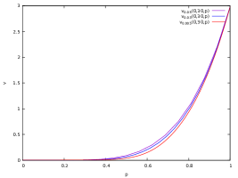
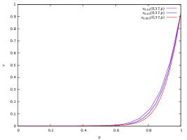
We observe, while not proved, that the numerical approximation always gives an upper bound for , which is itself greater than the quantile hedging price . This is a practically useful feature of this numerical method.
The scheme preserves a key feature of the exact solution, namely that the quantile hedging price is exactly for below a certain threshold, depending on . This is a consequence of the diffusion stencil respecting the degeneracy of the diffusion operator in (3.10), which acts only in direction , and by the specific construction of the meshes.
In Table 1, we show some discretisation parameters obtained by this construction with selected values of . Here, is the number of points for the -variable, the number of controls, and the total number of points for the variable (i.e., for all meshes combined). Moreover, (resp. ) is the greatest (resp. smallest) control obtained, using the modification of the control set (4.1) as described in Section 3.1. Also recall that different meshes are applied in each step of the PCPT algorithm for different , hence we also report (resp. ), the number of points for the variable for the control (resp. ). With our choice of parameters, we have , so the number of time steps is always .
| time (in seconds) | |||||||||
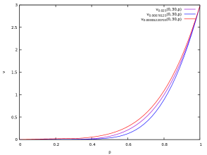
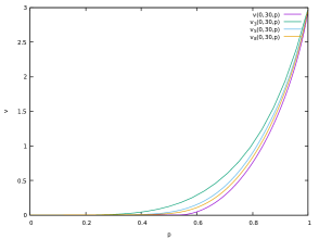
4.3 CFL conditions
Using the same discrete control set as above, we now fix and compute for chosen as above. The conditions (3.24) to (3.26) are then not satisfied anymore.
First, while is coarse, we observe that the computational time to get from is larger. In fact, since the conditions are not satisfied anymore, the results of Proposition 3.1 are not valid anymore. While convergence to a fixed point is still observed, many more Picard iterations are needed. For example, for and , we observe that Picard iterations are needed, while in the example where (3.24) to (3.26) were satisfied, iterations sufficed to obtain convergence (with a tolerance parameter of ).
The second observation is that, while we observe convergence to some limit (at least with our choice of : it might start to diverge for smaller , as seen for the case fixed and varying below), it is not the limit observed in the previous subsection. We show in Figure 3 the difference between the solution obtained with , and . When the conditions are not met, we are dealing with a non-monotone scheme, and convergence to the unique viscosity solution of the PDE, which equals the value function of the stochastic target problem, is not guaranteed.
Conversely, when is fixed and we vary , the situation is different. There is no issue with the Picard iterations, as the conditions needed for Proposition 3.1 are still satisfied. The issue here is that the consistency hypothesis is not satisfied, and convergence is not observed: when is too close to , the value gets bigger, as seen in Figure 3. Here, is fixed to and goes from to .

4.4 Convergence to the analytical solution with linear driver
We now consider the linear driver . In that case, the quantile hedging price can be found explicitly (see [19]). For each , the optimal control can also be computed explicitly:
where is the cumulative distribution function of the standard normal distribution.
In particular, if the uniform grid is fixed, one obtains that the optimal controls are contained in the interval .
On the other hand, if is fixed, one sees from (3.13) that the greatest control one can reach (with a non-trivial grid for the variable) is .
We set our parameters as follows: we first choose , we pick such that , and we set . It is easy to see that is proportional to .
We now pick the controls in to obtain as follows:
let so that . If are constructed, we set and . If , then we set and we are done.
In Figure 5, we observe convergence towards the quantile hedging price.
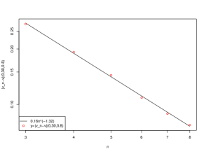
Moreover, Figure 5 demonstrates that the pointwise error, here for ,
has a convergence rate of about with respect to in the construction described previously.
Last, in Table 2, we report the values of and obtained for different choices of .
for .
5 Conclusions
We have introduced semi-discrete and discrete schemes for the quantile hedging problem, proven their convergence, and illustrated their behaviour in a numerical test.
The scheme, based on piecewise constant policy time-stepping, has the attractive feature that semi-linear PDEs for individual controls can be solved independently on adapted meshes. In the example of the Black-Scholes dynamics this had the effect that in spite of the degeneracy of the diffusion operator it was possible to construct on each mesh a local scheme, i.e. one where only neighbouring points are involved in the discretisation. This does not contradict known results on the necessity of non-local stencils for monotone consistent schemes in this degenerate situation (see e.g. [26]), because of the superposition of different highly anisotropic meshes to arrive at a scheme which is consistent overall.
6 Appendix
6.1 Proofs
Proof. [Proposition 3.3] For ease of notation, we set,
By the comparison theorem, it is enough to show that defined by
| (6.1) |
satisfies , and , for all and .
The boundary conditions are easily checked: if and
, we have, since :
For , , we prove . By definition (3.19), inserting , since and since is non-increasing with respect to its third variable and Lipschitz continuous with respect to its fourth variable, we have:
| (6.2) | |||
| (6.3) |
We have , thus:
| (6.4) | |||
It is thus enough to have
| (6.5) |
and one can easily check that this is the case with our choice of .
It remains to prove (3.42). Since for all , we have, by (3.26):
Proof. [Lemma 3.2]
We show the result for , the proof is similar for .
For and , let
| (6.6) |
It is enough to show that, for all and ,
Then, since is non-increasing in its third variable, it is then easy to show that satisfies (3.55).
Let and . We have, by definition
(3.19):
so it is enough to show
We split the sum into three terms:
First, we have
Secondly, by (3.15)-(3.16), we have,
The first term goes to since as and is bounded. The last three terms go to by Taylor expansion and Lemma 3.1, since is smooth.
Finally, by (3.15)-(3.16), using the linearity of the discrete differential operators and (6.6), and since is Lipschitz-continuous, we have,
We can show that each term goes to as . By example:
The first two terms go to with since and are bounded, by smoothness of and by Lemma 3.1.
We can control the derivatives of with respect to : for any , we have
| (6.7) |
for a constant .
By the triangle inequality and Taylor expansion, we get:
where , and this quantity goes to by our choice of .
Last, the smoothness of is straightforward by (3.54) and the control on its second derivative with respect to is obtained by (6.7).
6.2 Representation and comparison results
For , and , , denoting , we define, recalling (1.4)-(1.5)-(1.6),
where with a finite number of elements.
Proposition 6.1.
Let and (resp. ) be a lower semi-continuous super-solution (resp. upper semi-continuous sub-solution) with polynomial growth, of
| (6.8) |
with on , then on .
Corollary 6.1.
Proof. This is a direct application of the comparison principles. The equivalence between (6.8) and (6.9), comes from the fact that and have the same sign.
Lemma 6.1.
(i) Let and be the unique solution to
| (6.10) |
satisfying on , where . Then it admits the following probabilistic representation:
| (6.11) |
where is the first component of the solution to the following BSDE with random terminal time
| (6.12) |
with and
(ii) Assume moreover, that and , , with the notation of (2.14). Then the solution to
| (6.13) |
where , satisfies
Proof.
(i) The probabilistic representation is proved in [14]. Note that uniqueness to the PDE comes from the previous lemma in the special case where is reduced to one element.
(ii) Let , and , so that . For , let the solution to
By (2.14), we have for .
We introduce the following auxiliary processes, for ,
First, by construction, we have on . To prove the proposition it is thus sufficient to show that on . To this effect, we show that is solution of (6.13).
We have, for all ,
By our hypotheses and by the definition of , since on and on , we have
Thus, since , we deduce
Now, since on and on , and , we get
A similar analysis for the other terms shows that is a solution to (6.13) and concludes the proof.
6.3 Finite differences operator
We recall here the main results about the finite difference approximation defined by the operator , see (3.23).
Proposition 6.2 (Comparison theorem).
Proof. The proof is similar to the proof of Proposition 3.2 and is ommited.
Proposition 6.3.
Proof.
We only show the first point, the second one is obtained by applying the arguments of [4], after proving monotonicity, stability and consistency following the steps of Subsection 3.2.
Since is bounded, it is easy to show that is also bounded independently of , and the proof is similar to the proof of Proposition 3.6.
Since is Lipschitz-continuous, we get that is bounded. Using the Lipschitz-continuity of , one deduces easily that is a solution of
Again, comparison theorems can be proved, and it is now enough to show that there exists which are bounded uniformly in such that
We deal with only, we obtain similar results for .
One can easily show that , where , satisfies the requirements. Furthermore, one gets , thus one gets that is lower bounded by .
Acknowledgements
This work was partially funded in the scope of the research project “Advanced techniques for non- linear pricing and risk management of derivatives” under the aegis of the Europlace Institute of Finance, with the support of AXA Research Fund.
References
- [1] Yves Achdou, Guy Barles, Hitoshi Ishii, and Grigorii Lazarevich Litvinov. Hamilton-Jacobi equations: approximations, numerical analysis and applications, volume 10. Springer, 2013.
- [2] Guy Barles, Ch Daher, and Marc Romano. Convergence of numerical schemes for parabolic equations arising in finance theory. Mathematical Models and Methods in Applied Sciences, 5(1):125–143, 1995.
- [3] Guy Barles and Espen Jakobsen. Error bounds for monotone approximation schemes for parabolic Hamilton-Jacobi-Bellman equations. Mathematics of Computation, 76(260):1861–1893, 2007.
- [4] Guy Barles and Panagiotis E Souganidis. Convergence of approximation schemes for fully nonlinear second order equations. Asymptotic Analysis, 4(3):271–283, 1991.
- [5] Olivier Bokanowski, Benjamin Bruder, Stefania Maroso, and Hasnaa Zidani. Numerical approximation for a superreplication problem under gamma constraints. SIAM Journal on Numerical Analysis, 47(3):2289–2320, 2009.
- [6] Bruno Bouchard, Géraldine Bouveret, and Jean-François Chassagneux. A backward dual representation for the quantile hedging of Bermudan options. SIAM Journal on Financial Mathematics, 7(1):215–235, 2016.
- [7] Bruno Bouchard, Romuald Elie, and Antony Réveillac. BSDEs with weak terminal condition. The Annals of Probability, 43(2):572–604, 2015.
- [8] Bruno Bouchard, Romuald Elie, and Nizar Touzi. Stochastic target problems with controlled loss. SIAM Journal on Control and Optimization, 48(5):3123–3150, 2009.
- [9] Bruno Bouchard and Thanh Nam Vu. A stochastic target approach for P&L matching problems. Mathematics of Operations Research, 37(3):526–558, 2012.
- [10] Géraldine Bouveret and Jean-François Chassagneux. A comparison principle for PDEs arising in approximate hedging problems: application to Bermudan options. Applied Mathematics & Optimization, pages 1–23, 2017.
- [11] Jean-François Chassagneux and Adrien Richou. Obliquely reflected backward stochastic differential equations. 2018. ¡hal-01761991¿.
- [12] Michael G. Crandall, Hitoshi Ishii, and Pierre-Louis Lions. User’s guide to viscosity solutions of second order partial differential equations. Bulletin of the American Mathematical Society, 27(1):1–67, 1992.
- [13] Michael G. Crandall and Pierre-Louis Lions. Two approximations of solutions of Hamilton-Jacobi equations. Mathematics of Computation, 43:1, 1984.
- [14] Richard W.R. Darling and Etienne Pardoux. Backwards SDE with random terminal time and applications to semilinear elliptic PDE. The Annals of Probability, 25(3):1135–1159, 1997.
- [15] Roxana Dumitrescu. BSDEs with nonlinear weak terminal condition. arXiv preprint arXiv:1602.00321, 2016.
- [16] Roxana Dumitrescu, Romuald Elie, Wissal Sabbagh, and Chao Zhou. BSDEs with weak reflections and partial hedging of American options. arXiv preprint arXiv:1708.05957, 2017.
- [17] Roxana Dumitrescu, Christoph Reisinger, and Yufei Zhang. Approximation schemes for mixed optimal stopping and control problems with nonlinear expectations and jumps. arXiv preprint arXiv:1803.03794, 2018.
- [18] Nicole El Karoui, Shige Peng, and Marie-Claire Quenez. Backward stochastic differential equations in finance. Mathematical finance, 7(1):1–71, 1997.
- [19] Hans Föllmer and Peter Leukert. Quantile hedging. Finance and Stochastics, 3(3):251–273, 1999.
- [20] Emmanuel Gobet and Stefano Pagliarani. Analytical approximations of BSDEs with nonsmooth driver. SIAM Journal on Financial Mathematics, 6(1):919–958, 2015.
- [21] Espen R. Jakobsen and Kenneth H. Karlsen. Continuous dependence estimates for viscosity solutions of integro-PDEs. Journal of Differential Equations, 212(2):278–318, 2005.
- [22] Espen R. Jakobsen, Athena Picarelli, and Christoph Reisinger. Improved order 1/4 convergence for piecewise constant policy approximation of stochastic control problems. arXiv preprint arXiv:1901.01193, 2019.
- [23] Nikolaj V. Krylov. Approximating value functions for controlled degenerate diffusion processes by using piece-wise constant policies. Electronic Journal of Probability, 4(2):1–19, 1999.
- [24] Nikolaj V. Krylov. On the rate of convergence of finite-difference approximations for Bellmans equations with variable coefficients. Probability Theory and Related Fields, 117(1):1–16, 2000.
- [25] Ludovic Moreau. Stochastic target problems with controlled loss in jump diffusion models. SIAM Journal on Control and Optimization, 49(6):2577–2607, 2011.
- [26] Christoph Reisinger. The non-locality of Markov chain approximations to two-dimensional diffusions. Mathematics and Computers in Simulation, 143:176–185, 2018.
- [27] Christoph Reisinger and Peter A. Forsyth. Piecewise constant policy approximations to Hamilton-Jacobi-Bellman equations. Applied Numerical Mathematics, 103:27–47, 2016.
- [28] Xavier Warin. Some non-monotone schemes for time dependent Hamilton–Jacobi–Bellman equations in stochastic control. Journal of Scientific Computing, 66(3):1122–1147, 2016.