Enlightening force chains: a review of photoelasticimetry in granular matter

Abstract

A photoelastic material will reveal its internal stresses when observed through polarizing filters. This eye-catching property has enlightened our understanding of granular materials for over half a century, whether in the service of art, education, or scientific research. In this review article in honor of Robert Behringer, we highlight both his pioneering use of the method in physics research, and its reach into the public sphere through museum exhibits and outreach programs. We aim to provide clear protocols for artists, exhibit-designers, educators, and scientists to use in their own endeavors. It is our hope that this will build awareness about the ubiquitous presence of granular matter in our lives, enlighten its puzzling behavior, and promote conversations about its importance in environmental and industrial contexts. To aid in this endeavor, this paper also serves as a front door to a detailed wiki containing open, community-curated guidance on putting these methods into practice Zadeh et al. (2019).

1 Introduction

Most of the transparent objects we encounter are photoelastic: their degree of birefringence depends on the local stress at each point in the material Frocht (1969); Cloud (1995). This property can be used to visualize, and even quantitatively measure, what is usually invisible to our naked eye: the stress field. When such materials are subjected to an external load, and placed between crossed polarizing filters, each different region of the material rotates the light polarization according to the amount of local stress Daniels et al. (2017). This creates a visual pattern of alternating colored fringes (see Fig. 1) within the material which, on top of their aesthetic and pedagogical aspects, permits us to quantify the stress field within the material.

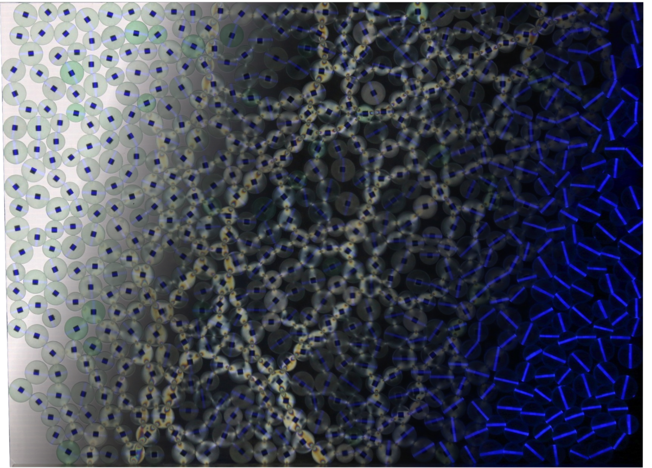
Figure 1: Composite view of a granular photoelastic system. On the left side, the grains are imaged with white backlighting. In the middle, the particles are viewed between crossed polarizers, revealing the force chains through photoelasticity. On the right side, the system is imaged from above with a UV light, revealing inked bars used to track particle rotation. Within each particle, an embedded cubic magnet is visible as a dark square Cox et al. (2016).

Photoelastimetry has its roots in engineering practice, where it was widely used to design parts before the rise of computational finite element methods Cloud (1995). It also provided the first glimpse of the internal forces within granular materials, at first qualitatively Wakabayashi (1950); Dantu (1957); A and Josselin (1972); Liu et al. (1995) and later quantitatively Howell et al. (1999); Majmudar and Behringer (2005). Today, it remains the most well-developed method for quantifying stresses Amon et al. (2017), and methods for particle making Cox et al. (2016); Barés et al. (2017a) and image post-processing Daniels et al. (2017); Kollmer (2018); Lantsoght and Docquier (2018) are under active development.

After two decades of quantitative efforts, the scientific successes of the photoelastimetry method are numerous. In Robert Behringer’s group alone, it was responsible for identifying the erratic stress fluctuations in sheared granular matter Howell et al. (1999); Barés et al. (2017b); Zadeh et al. (2018), Green’s function response Geng et al. (2001), particle-scale anisotropy of the contact force networks Majmudar and Behringer (2005); Zhang et al. (2010), shear jamming Majmudar et al. (2007); Bi et al. (2011); Ren et al. (2013); Zheng et al. (2014); Wang et al. (2018), the dynamics of granular matter under impact Clark et al. (2012); Lim et al. (2017); Zheng et al. (2018), the Reynolds pressure, the Reynolds coefficient Ren et al. (2013), and more.

Far beyond the bounds of his laboratory at Duke University, the method has been used to examine particle shape dependence Zuriguel and Mullin (2008), identify interparticle contacts Lherminier et al. (2014), observe sound propagation Shukla (1991); Owens and Daniels (2011); Huillard et al. (2011), test the validity of statistical ensembles Puckett and Daniels (2013); Bililign et al. (2019), examine sensitivity to initial conditions Kollmer and Daniels (2018), identify dilatancy softening Coulais et al. (2014), measure force chain order parameters Iikawa et al. (2016), and observe the effects of fluid flow Mahabadi and Jang (2017). In interdisciplinary efforts, photoelastimetry permits scientists to evaluate the grain-scale stresses caused by growing plant roots Wendell et al. (2012); Kolb et al. (2012); Barés et al. (2017a), and examine situations relevant to faulting and earthquakes Daniels and Hayman (2008); Hayman et al. (2011); Geller et al. (2015); Lherminier et al. (2019)

The structure of the paper is as follows. First, we briefly review the physics of photoelasticity in §2; this section can be skipped for those only interested in qualitative uses of the method. In §3, we present various ways of fabricating photoelastic particles by cutting, casting or printing, followed by imaging-techniques in §4; these two section can stand alone for the creation of a demonstration apparatus. Finally, we present quantitative methods in §5. In all cases, additional information and technical specifications are provided on a wiki to which many of the paper authors have contributed Zadeh et al. (2019).

2 Photoelasticimetry theory

Photoelasticity arises from the birefringent properties of most transparent materials, in which the speed of light (via the index of refraction) depends on the polarization of the incident light wave. In some cases, such as glass and polymeric materials, birefringence arises only when the material is subject to anisotropic stress, with the refractive indexes depending on the eigenvalues of the local stress tensor. As such, photoelasticity can provide measurements of the internal stress in the material.

Measurements are best taken using circularly (rather than linearly) polarized light, in order to provide isotropic measurements. Circularly polarized light is created using a linear polarizer followed by a quarter-wave ($\pi/2$) phase shift between the two orthogonal components, as shown in Fig. 2. On the other side of the birefringent material, a circular polarizer with opposite polarity (the “analyzer”) blocks any light that doesn’t match its polarization. If the material is unstressed, there is no transmitted light and a dark image results. However, anyplace in the material where there is anisotropic stress, the wave components which are polarized along the two principle axes of the local stress tensor will travel with different speeds. This speed difference results in a relative phase shift for these two components of the wave, converting circularly polarized light to elliptically polarized light. As a consequence, a portion of the wave is not completely blocked by analyzing polarizer, and is therefore recorded as a bright region of the image.

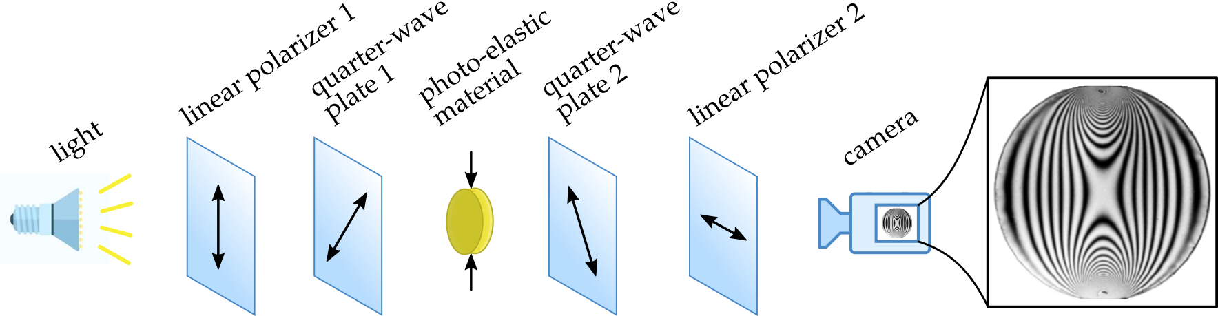
Figure 2: Schematic image of the photoelastic technique for a darkfield transmission polariscope: the combination of linear polarizer $1$ and quarter-wave plate $1$ (with a $\pi/4$ difference of principle directions), converts unpolarized light into circularly polarized light. This light passes through a uniaxially loaded photoelastic particle. A second combination of plate $2$ and linear polarizer $2$ (producing the opposite chirality) blocks any un-rotated light. At locations where there are anisotropic stresses in the photoelastic material, there will be different phase shifts for different components of the light wave; this phase shift changes the polarization of the light wave, causing these locations to appear bright in a camera image (or by eye). A sample image obtained with monochromatic light is given on the right hand side of the figure; each fringe is produced by an integer number of rotations of the polarization of light through a phase of $\pi$, as given by Eq. 3.

This property allows photoelasticity to be used to quantitatively measure local stress, via an inverse method. We begin by assuming that the relation between the local stress and the refractive index is linear. We consider the difference in transmission between the two principle axes:

$$n_{1}-n_{2}=C(\sigma_{1}-\sigma_{2}),$$ (1)

where $\sigma_{1},\sigma_{2}$ are the two eigenvalues of the local stress tensor, and $n_{1},n_{2}$ are the two refractive indices in the corresponding directions. The material constant $C$ is known as the stress-optical coefficient. The relative phase shift of wave components in the eigendirections of the local stress tensor is determined from

$$\alpha=\frac{2\pi Cd}{\lambda}(\sigma_{1}-\sigma_{2}),$$ (2)

with $\lambda$ the wavelength of the incident light and $d$ the distance traveled inside the material (its thickness). For this phase shift, the intensity of the wave that emerges from the analyzer is given by

$$I=I_{0}\sin^{2}\frac{\alpha}{2}=\sin^{2}\left[\frac{\pi Cd}{\lambda}(\sigma_{1}-\sigma_{2})\right].$$ (3)

More details about these relationships and how to calibrate the material parameters for quantitative measurements can be found in Trushant S Majmudar (2006); Daniels et al. (2017) and §5.

Note that while Eq. 3 relates internal stress and image intensity for a single wavelength of light, the effect is also preset for a superposition of wavelengths (e.g. white light), as shown in Fig. 1. The difficulty is that inverting Eq. 3, to infer local stress from light intensity, requires the use of a single wavelength in order to be tractable. Even so, the non-uniqueness of the solution due to the $\sin^{2}$ term makes the inversion problem challenging. §5 of this paper provides techniques for performing this task.

3 Fabricating photoelastic particles

While many transparent materials have photoelastic properties, only some of them have a large enough value of the stress-optical coefficient $C$ (see Eq. 1) to produce a measurable effect under reasonable loads. Furthermore, it is necessary to pay special attention during the fabrication of a material in order not to create an object containing significant residual stresses. Therefore, the creation of a photoelastic granular material requires considering all of the following: (1) the load you will to apply; (2) whether the shape of the particles matters; (3) how precisely you expect to make quantitative measurements, if at all; (4) what imaging method you will use; and (5) budget available. In this section, we explain several ways to meet these goals, ranging from simply cutting particles from pre-existing sheets up to casting bespoke particles.

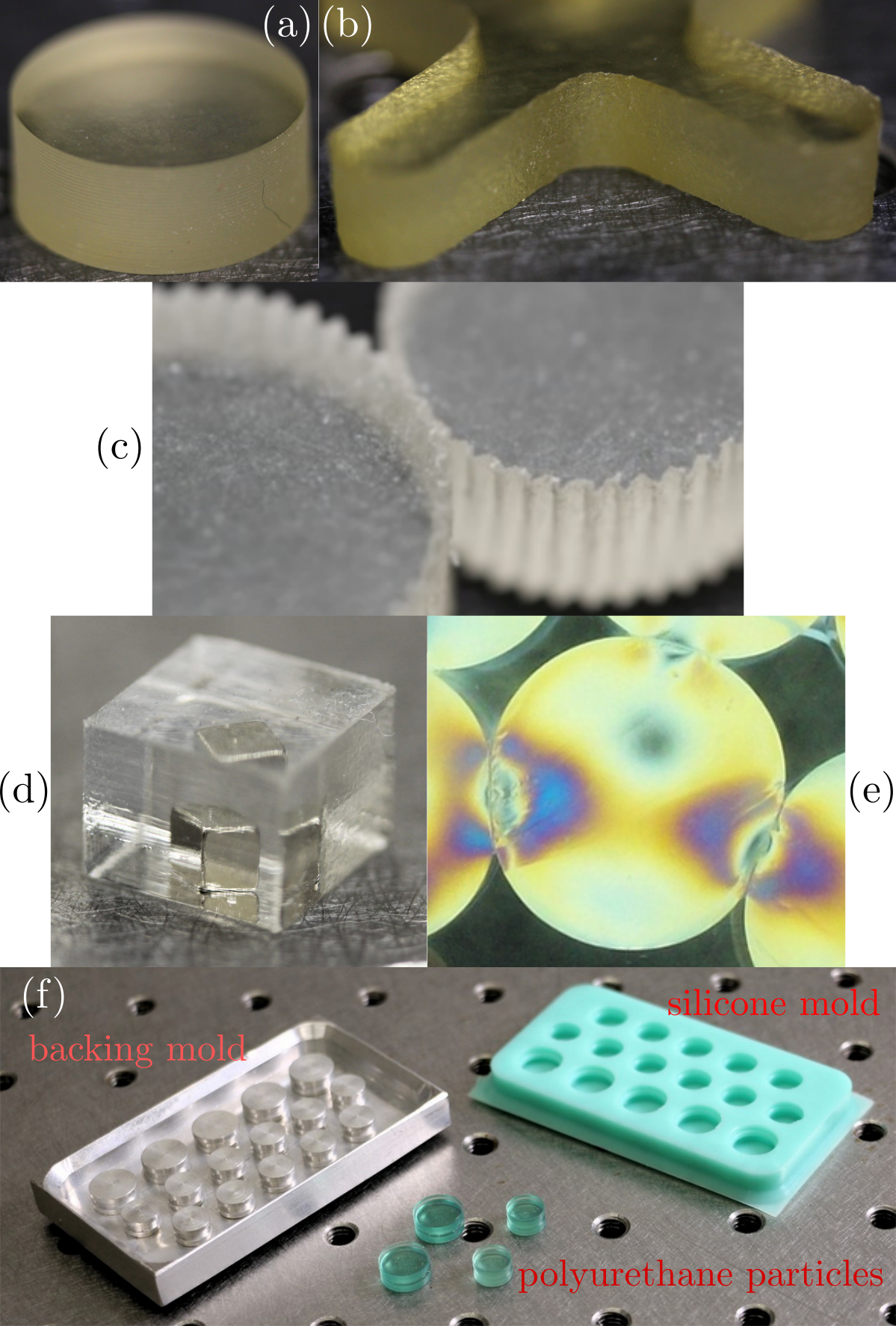
Figure 3: (a) Disc cut out of a photoelastic sheet pre using a rotating cookie cutter. (b) Cross-shaped particle cut out of a photoelastic sheet pre using a computer-controlled milling machine. (c) Geared particles cut out of a photoelastic sheet pre using a computer-controlled waterjet. (d) Cast polyurethane cle particle containing a magnetic inclusion. (e) Molded gelatin discs observed through crossed polarizers. (f) Backing mold, mold and urethane cast photoelastic particles. All the particles are approximately 1 cm in size.

Before choosing the material for the particles, it is important to consider that the photoelastic signal is a periodic function of the stress (see Eq. 3). The larger the deformation, the higher the stress, and the larger the number of fringes will be observed (see example in Fig. 2). Therefore, increased material stiffness is required for experiments with larger load, so that the fringes do not become denser than the resolution of the imaging system. Conversely, if the material is too stiff (or the loading too weak, or the thickness too small), then insufficient photoelastic signal will be observed. It is therefore advisable to perform some preliminary trials before committing to a large batch of particles.

3.1 Cutting sheets

Historically, it was simplest to make photoelastic particles by simply cutting shapes out of a pre-existing sheet of photoelastic material. This could be a flat sheet of Plexiglas^™ or a rubber, which is then cut with a bandsaw (the original Behringer particles), milling machine, spinning cookie cutter, or waterjet. The choice of material needs to match the experimenter’s dual requirements of deformability and sensitivity ($C$ in Eq. 1), to be compatible with the intended applied load. Most commonly, it is convenient to simply purchase sheets of transparent Vishay PhotoStress^™ vis or polyurethane pre , but for high loads Plexiglas^™ or polycarbonate are also suitable choices. The stiffer materials can be machined using any appropriate tool, with residual stresses annealed out by heating them to just below their glass transition temperature. In all cases, a diversity of thickness, stiffness, and color are available. Sheets of thickness $1/4$” and hardness $60$A are quite broadly-applicable, such that some particles of this type remain in use after two decades of use Howell et al. (1999); Barés et al. (2017b).

If circular-shaped particles (discs) are desired, a custom-built “cookie cutter” tool can make numerous, identical particles from a single sheet with little waste Daniels et al. (2017). Both the rotation and downward cutting speeds have to be properly chosen as a function of the material not to induce residual stresses when cutting. An example of particle obtained with this method in given in Fig. 3a, with slight horizontal marks made by the cutter. For more complicated shapes (see Fig. 3b), a computer-controlled milling machine outfitted with a narrow-diameter mill can trace arbitrary outlines, again with care taken to minimize residual stresses. In this case, there is also some roughness at the outer surface. Finally, it is possible to create arbitrary shapes with waterjet cutting, first used by Wendell et al. (2012) and further developed by Wang (2018). Depending on the skill of the operator, the resulting particles can have straight and smooth edges with few residual stresses, but can also sometimes leave a narrow channel at the start/end point of the cut. The narrow cutting width of the waterjet ($\sim 0.1$ mm) has the benefit of permitting very complex edges, as shown in Fig. 3c.

3.2 Casting particles

A second method to make photoelastic particles is to mold them directly, from such materials as polyurethane, gelatin, or nearly any other castable polymer or water gel. This allows an even larger diversity of complex, 3D shapes Barés et al. (2017a) so long as a mold can itself be fabricated. Using this method, it becomes possible to tune the stiffness (via the controlled addition of crosslinking molecules) or to add inclusions Cox et al. (2016) as shown in Fig. 3d.

The first step of the casting method requires creating a backing mold: a positive relief of the desired particle shape. The backing mold can be machined or 3D printed of nearly any material stiff enough to maintain a shape. As shown in Fig. 3f, this backing mold is then used to cast the final (reusable) silicone mold that makes the actual particles. A commercial silicone mold formulation such as MoldStar^™ provides easy-to-use formulations mol ; we have found that 15 Slow fits most needs.

Urethane is one popular choice of particle material Barés et al. (2017a). The commercial product ClearFlex^™ cle is available in different stiffnesses ($50$A fits most needs), and it can be custom-tuned by varying the crosslinker ratio. For the benefit of particle-tracking (see §5.1), it can be helpful to dye the clear urethane (see Fig. 5). The product SoStrong^™ so_ provides suitable dyes. Casting urethane requires some care to avoid the production of bubbles, compensate for material shrinkage, and develop fast enough work-flows; a number of helpful tricks from the community are shared at the online wiki Zadeh et al. (2019).

Another popular choice is to use biological gels which are cheap and easy to use, but non-permanent. As shown in Fig. 3e, gelatin has excellent photoelastic properties Kilcast et al. (1984); Lim et al. (2017); Workamp et al. (2017), as does agar or konjac Tomlinson and Taylor (2015) (with the later being less transparent). The stiffness of these materials is easy to tune by varying the ratio of gelling agent, and it is possible to achieve arbitrarily low elastic moduli. However, because biological gels are composed of water and a food source, they are vulnerable to drying, swelling, and bacteria; so they are not stable over long times. Some groups have had success by crosslinking the gel Damink et al. (1995); Workamp et al. (2016) when making particles Workamp et al. (2016). In this case, glutaraldehyde is directly added to the liquid gelatin preparation before molding or it can be diffused into the gelatin particles once they have gelled Workamp et al. (2016) to increase the particle stiffness and stabilize the material.

3.3 3D printing particles

Finally, when the particle shape is sufficiently complex that a backing mold cannot be made, it is possible to simply 3D print individual photoelastic particles. This choice is not as straightforward as it might seem, since most of the available printing materials are non-transparent, porous, and contain residual stresses. However, optical fabrication processes (stereolytography) now allow for the production of semi-transparent photoelastic particles. Two available options are Durus White^™ used by Lherminier et al. (2016), and VeroClear^™ ver used by Wang et al. (2017). The VeroClear has better clarity and optical response, but both are quite stiff and are therefore only appropriate for experiments with large loading stresses.

4 Imaging methods

In designing a photoelastic experiment, it is also necessary to consider the imaging method. The most appropriate choice will depend on considering the magnitude of the photoelastic response (§2) for the applied load, as well as desired degree of precision and the speed with which the images need to be collected to capture the dynamics. In this section, we elucidate several different methods that allow for adapted to a variety of constraints.

4.1 Transmission vs. reflection imaging

In §4 and Fig. 2, we considered a geometry in which the light is transmitted directly through the particles from a polarized light source, and then through a second filter (analyzer) before reaching the camera. In cases where the experiment will be optically-accessible from both sides of the particles, this is the easiest polariscope to construct, and has seen the most usage over the past several decades Liu et al. (1995); Majmudar and Behringer (2005); Daniels et al. (2017). Care must be taken when constructing the optical pathway of filters, that the polarizers be perfectly crossed and aligned exactly as shown in Fig. 2. This can be done either by purchasing two pairs of linear polarizers and quarter-wave plates pol and doing the alignment by hand, or by purchasing a pair of left and right circular polarizers which are pre-aligned sandwhiches containing both components. In that case, care must be taken to orient the quarter-wave plate side of the polarizer towards the granular material so that light passes through the filters in the correct sequence. If the circular polarizers are pre-mounted inside a camera filter, their default configuration will be backwards from what is required for the polariscope shown in Fig. 2.

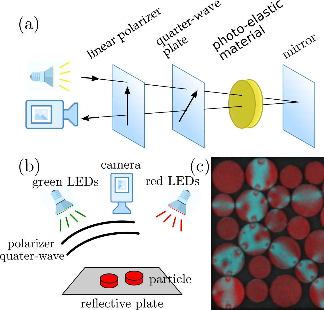
Figure 4: Schematic of the reflective photoelastic technique Daniels et al. (2017). (a) As for the transmission method (Fig. 2), the combination of linear polarizer and quarter-wave plate converts unpolarized light into circularly polarized light. In this case, however, the reflector on the back side of the particle both creates the round-trip, and also reverses the polarization of the light. Therefore, there is only one polarizer that also serves as the analyzer. (b) Sample reflective photoelastic set-up, illuminated with both a green polarized light and red unpolarized light. (c) Sample image from Kollmer and Daniels (2018), recorded with a reflective polariscope of the type shown in (b). To render this red-green image accessible to more readers, the green channel has been copied into the blue channel.

In some cases, the granular material may not be optically-accessible from both sides, for instance due to the loading mechanism or because the particles are resting on an opaque surface Puckett and Daniels (2013); Zhao et al. (2017). It can therefore be desirable to create an optical setup in which the the apparatus is lit and imaged from the same side: this is a reflective polariscope. As in transmission polariscope, both the polarizer and the analyzer are circular, but now a single polarizer serves in both roles (see Fig. 4). Two successful options for reflecting the polarized light back through the granular sample are to rest the particles on a mirrored surface, or to coat all particles with a mirror-effect paint. Details about how to construct such an apparatus are provided in Daniels et al. (2017).

4.2 Multi-wavelength imaging

As described by Eq. 3, quantitative stress measurements require monochromatic light measurements. In order to minimize the overlapping of photoelastic fringes at high stresses (as can seen in Fig. 2), it is important to work with monochromatic light. Furthermore, polarizers and quarter-wave plates are optimized for a given wavelength, usually green light. Therefore, a quantitative apparatus should be designed so that green light is used for photoelastic measurements, and other wavelengths are used for monitoring quantities such as particle positions and orientations.

One method, suitable for quasi-static dynamics, is to perform sequential imaging after each loading step Ren et al. (2013); Barés et al. (2017b); Zhao et al. (2017). For example, the camera takes an image (1) between crossed polarizers, to observe the photoelastic response; (2) without at least one of the polarizers, to detect particle positions; and (3) additionally illuminated by UV light, to monitor an additional characteristic such as particle orientation. An example of this type of imaging is shown in Fig. 1 and Fig. 6d, in which a bar drawn in UV-sensitive ink is visible.

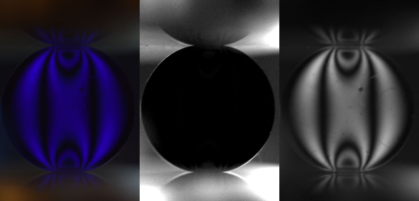
Figure 5: A photoelastic particle dyed dark blue acts as wavelength filter. (Left) A color image of the particle illuminated by white light in a transmission polariscope can be split such that (middle) the green channel provides a brightfield image of a black disk, suitable for location detection, and (right) the blue channel provides a darkfield image of the photoelastic response.

Another option is to measure these same fields simultaneously, by choosing to illuminate different properties using different wavelengths of light. Conveniently, color cameras already perform color-separation into red, green, and blue (RGB) channels. For example, the particle positions can be illuminated in unpolarized red light, while the photoelastic measurements are recorded by polarized green light, and a subset of tagged particles identified by UV-ink tags that emit blue light Puckett and Daniels (2013); Kollmer and Daniels (2018). Such a setup is shown schematically in Fig. 4b, with a sample image in Fig. 4c.

A third approach is to use dyed particles, which can then be illuminated with white light. In this case, the particles effectively act as a bandpass filter, and the passed wavelength can be used to make photoelastic measurements while blocked wavelengths provide position data. A particle dyed dark blue is shown to demonstrate this effect in Fig. 5. These techniques allow a single image to provide both position detection and stress measurements at the same instant in time, making it possible to monitor the dynamics of a system.

5 Analyzing images

We have seen numerous examples of photoelastic images taken from a variety of geometries and lighting conditions; next, we examine several key methods of extracting quantitative information from such images. The level of precision available to the user – whether particle position, orientation, or force – depends on the focus and resolution of the images, the photoelastic sensitivity of the particles (parameter $C$ in Eq. 1), and the magnitude of the applied load. In what follows, we will focus on the use of cylindrical (disk) particles.

5.1 Tracking particle positions and orientations

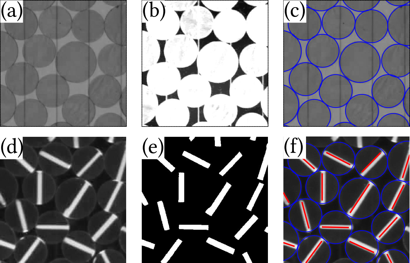
Figure 6: (a-c) Examples of locating particle-centers and measuring their diameters: (a) one channel of a originally-white light image, (b) enhanced contrast image with background noise removed, and (c) tracked particles shown as blue circles, found using the circular Hough transform method. (d-f) Examples of tracking particle orientations: (d) blue channel of a original UV light image, (e) enhanced contrast image with background noise removed, and (f) tracked orientations marked by red lines.

For particle detection, the first step is to produce a high-contrast (even binary) image to distinguish the pixels occupied by particles from those that are not. This is best done on whichever color-channel (red, green, or blue) has the highest contrast between the particles and their background. It can be helpful to increase the contrast by filtering single high/low outlier pixel values (see Fig. 6a), and also to apply a low-pass Fourier filter (see Fig. 6). These steps work for particles of any shape.

Starting from a filtered image improves particle-finding methods, of which we will consider the two most convenient: convolutions Shattuck (2015) and Hough transforms. If the particles are not circular, then the convolution method is preferred over the Hough transform; it can also achieve higher precision but is more computationally-intensive. Image convolutions are performed between a pre-set image (“kernel”) of a single ideal particle (approximately $3/4$ the diameter of the smallest particle works well), and the original or binarized image. After performing the convolutions, binarizing the resulting image using a threshold of $99.5\%$ of the peak convolution value will result in a field of well-isolated peaks corresponding to the particle centers, with the area of each peak indicating that particle’s diameter. For circular (non-binarized) images, it is possible to use a circular Hough transform to locate the particle centers and sizes Peng et al. (2007); Puckett and Daniels (2013). This transform works best on an image that has been prepared, via edge-detection, to isolate the circumference of particle. The algorithm uses a computationally-efficient voting process to identify the centers of such circles of a specified radius. A sample result of particle-detection via the Hough transform in shown in Fig. 6c.

From the the list of particle centers present in each image of a series, it is possible to track Lagrangian trajectories of those particles through space and time. Two efficient, accurate, and open-source algorithms are those of Crocker and Grier (1996) and Blair and Dufresne . The main idea for both is that, given the positions for all detected particles at a given step, the aim is to select the closest possible new positions from the list of all detected particles in the next step. To this end, the algorithm considers all possible pairings of (old-new) positions, and selects the pairing that would result in the minimal total squared displacement. If a particle is missed over a small interval, the two halves of the trajectory later be re-attached. In cases where the image resolution was insufficient to reliably detect particle positions, it is still possible to use particle image velocimetry (PIV) to measure Eulerian flow fields for a series of images Willert and Gharib (1991).

Finally, it is possible to tag the particles with a contrasting stripe, in order to measure particle-rotation during dynamics. One common method, shown in Fig. 6d-f, is to mark the top of each particle with a UV ink bar. This ink is not visible under white light, and therefore doesn’t interfere with ordinary particle-tracking as described in the first part of this section. However, once illuminated by UV light alone, the ink bars become visible with high enough contrast to be recorded by a camera. The contrast is sufficient to binarize the image, and the position of each particle center can be used to conduct a least squares of the bar pixels in order to determine its orientation (see Fig. 6f).

5.2 Scalar measurements of force

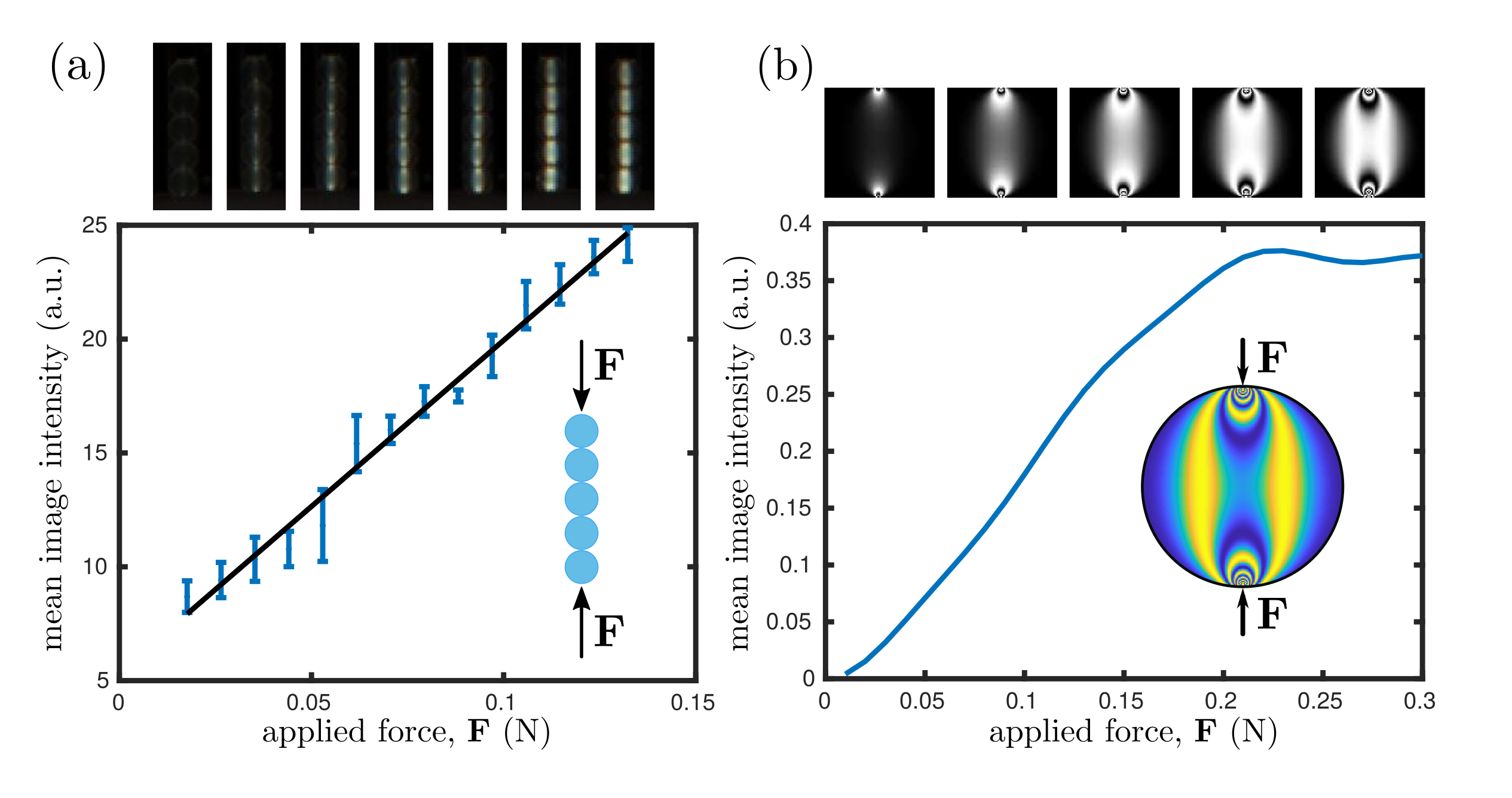
Figure 7: Calibration curve for mean image intensity on (a) experiments and (b) numerical simulations of diametrically-loaded disks, as a function of applied force. Numerical simulultions are based on the stress field inside a single disk Landau and Lifshitz (1986), and the photoelastic response (Eq. 3) is computed over a domain of $20\times 20$ pixels, with $Cd=70$ m²/N. Images corresponding to the different forces are shown on top of the diagram. The error bars are standard deviation on mean.

For many experiments, it is desirable to make quick, low-resolution measurements of the forces on each particle, rather than solving the full inverse problem to obtain vector contact forces as will be described in §5.3. Scalar measurements can be the best choice for a variety of reasons: poor image resolution, dim lighting, fast dynamics, or a very large number of images. It is the easiest analysis when beginning a new project, as a tool for preliminary investigations, and remains popular because if its computational efficiency.

The simplest form of scalar analysis is to use the mean light intensity within particles. For small forces, the mean image intensity increases linearly with the applied force, as shown in Fig. 7a for a sample experiment under a known imposed load. By analyzing a small system such as a linear chain, it is possible to perform a calibration which provides a quantitative measure of the force on particle. As shown in Fig. 7b for a numerical version of this calibration, there is a threshold force above which the mean light intensity plateaus and this method is no longer quantitative. This threshold corresponds approximately to the development of the first additional set of fringes. For applied forces within the linear regime, this method is valid.

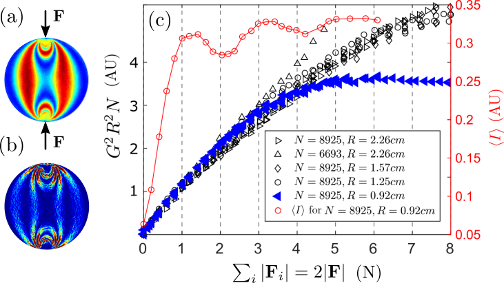
Figure 8: (a) Light intensity $I(i,j)$ of a diametrically loaded disk with force $\vec{F}$ between crossed polarizers. (b) The calculated $|\nabla I|^{2}$ distribution from (a). (a) and (b) are colored by the magnitude of $I$ and $|\nabla I|^{2}$ respectively. (c) Dependence of $G^{2}$ and averaged light intensity $\braket{I}$ on the contact forces for diametrically loaded disks with different $R$ (disk radius) and $N$ (number of pixels per meter) while keeping other experimental parameters the same. $\braket{}$ means averaging over pixels inside the disk. The black and blue data shows collapse of $G^{2}$ after proper rescaling using $R$ and $N$. The saturation forces for intensity and $G^{2}$ for an example run are about $1$ N and $4$ N respectively, showing that $G^{2}$ measures much larger range of forces. Data from Zhao et al. (2019).

Once this threshold is crossed, the variation in intensity due to the fringes becomes a significant factor, allowing for an additional quantitative technique which accounts for the presence of the fringes. For images at high enough resolution to observe fringes, the force on the particle can be measured using the gradient of the image intensity field $I(i,j)$, known commonly as the $G^{2}$ technique. It is defined as follows:

$$\begin{array}[]{l}G^{2}\equiv\braket{}{\nabla I_{i,j}}{{}^{2}}=\frac{1}{4}\langle[(I_{i-1,j}-I_{i+1,j})^{2}/4\\ +(I_{i-1,j-1}-I_{i+1,j+1})^{2}/8+(I_{i,j-1}-I_{i,j+1})^{2}/4\\ +(I_{i+1,j-1}-I_{i-1,j+1})^{2}/8]\rangle\end{array}$$ (4)

where $i$ and $j$ refers to the row and column number of pixels and $\braket{\cdot}$ means averaging over pixels in the region of interest Majmudar (2006). Figs. 8 shows the distribution of light intensity $I$ (a) and its squared gradient $|\nabla I|^{2}$ (b) for a photoelastic disk under normal compression.

This method has been used to measure both the average pressure for the whole image Howell et al. (1999); Geng et al. (2001); Farhadi and Behringer (2014); Zheng et al. (2014); Farhadi et al. (2015); Cox et al. (2016); Daniels et al. (2017); Zheng et al. (2018), and at the particle scale Clark et al. (2012); Coulais et al. (2014); Iikawa et al. (2015); Barés et al. (2017b); Wang et al. (2018). For bulk measurements, we observe that $G^{2}$ is a monotonic function of pressure, with some nonlinearity in the relationship Howell et al. (1999). For particle-scale measurements on disks, if applied forces are small enough such that photoelastic fringes can be clearly resolved, $G^{2}$ is proportional to the sum the individual vector contact forces $\sum_{i}|\vec{F}_{i}|$, where ${\vec{F}}_{i}$ are the contact forces on the disk Zhao et al. (2019) (see Fig. 8a). Thus, where tangential forces are not large, $G^{2}$ approximately measures the particle scale pressure.

Importantly, $G^{2}$ will differ based on the material choice, the lighting condition and the image resolution. At particle scale, for an individual disk, the coefficient of proportionality $k=G^{2}/\sum_{i}|\vec{F_{i}}|$ is shown to be proportional to $I_{0}^{2}Cd/\lambda R^{2}N$ Zhao et al. (2019), with $\lambda$ the light wavelength, $C$ the stress-optical coefficient, $d$ the disk height, $R$ its radius, $N$ the camera resolution defined as number of pixels per meter and $I_{0}$ the background light intensity. As an example, Fig. 8c plots the collapse of the linear part of $G^{2}$ rescaled using $N$ and $R$ as functions of $\sum_{i}|\bf{F_{i}}|$ for diametrically loaded disks (see Fig. 8a) with other parameters kept the same. The dependence of $G^{2}$ on $R$ is important for analyzing poly-disperse systems. Fig. 8c also compares the dependence of $G^{2}$ and intensity $I$ on the contact forces for a given test, showing that the range of force that $G^{2}$ can measure is $4$ to $5$ times larger than that of $I$. Note that the linear dependence of $G^{2}$ value for individual disk on contact forces will differ for other particle shapes Zhao et al. (2019).

5.3 Vector measurements of force

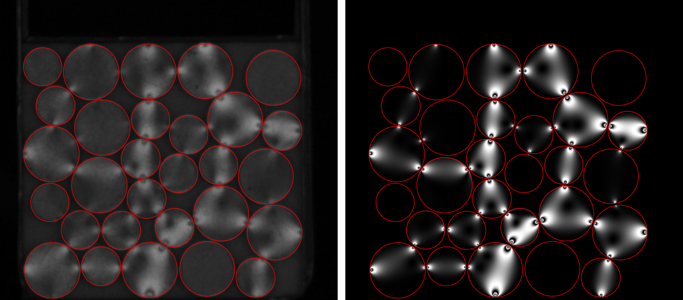
Figure 9: Experimental photoelastic response (left side) and numerically generated counterpart (right side) after the optimization of all ${\vec{F}}_{i}$ contact forces. Data from Kollmer (2018).

The detailed pattern of light and dark fringes in $I(i,j)$ is set by the local stress values through Eq. 3. Therefore, it is possible to use a known stress field (computed from the set of vector contact forces ${\vec{F}}_{i}$) to predict a light intensity field. Examples of such calculations are shown in Fig. 7b. In order to determine the values for each ${\vec{F}}_{i}$ from the fringe pattern requires performing the inverse of this process, as illustrated in Fig. 9. Because Eq. 3 cannot be directly inverted due to the $\sin^{2}$ non-monotonic function, the numerical estimation of the set of ${\vec{F}}_{i}$ must be done via an optimization process. This is achieved in a sequential process:

1. Detect the particle positions (see §5.1)

2. Estimate the total and individual contact force magnitudes on each particle (see §5.2)

3. Optimize ${\vec{F}}_{i}$ on each particle according to a set of constraints

Note that the second step contains two parts. It is usually possible to use the $G^{2}$ method to estimate the total force, but this may not be possible for the individual contacts, depending on the image resolution. If the quality of the photoelastic image is good enough, each contact force can be similarly estimated from calculating $G^{2}$ in the vicinity of each contact Daniels et al. (2017); Kollmer (2018). This method allows for the removal of contacts that do not transmit loads, and for the inverse problem to be performed on individual particles. However, the contact-scale step is not always possible for lower-resolution images, for example in the case of stirred granular media Lantsoght (2019). Instead, the optimization step (below) must also include a process for testing multiple different contact-configurations in which the total force magnitude is taken to be equally-distributed in the initiation of the optimizer Lantsoght and Docquier (2018).

The third step proceeds to optimize the vector contact forces ${\vec{F}}_{i}$, starting from the estimated values in steps 1 and 2, in order to achieve a photoelastic response as close as possible to the image intensity $I(i,j)$. The input (initial guess) and output (optimized) parameters are therefore the set of all contact force magnitudes and orientations. For cylindrical, linearly-elastic particles subjected to multiple contact forces, the stress-field can be approximated by an analytical expression Timoshenko and Goodier (1970); Daniels et al. (2017).

Combining this stress field with Eq. 3 creates a reconstructed image of each particle which can be evaluated against the measured image. The chosen optimization algorithm works by evaluating the agreement between these two images – the measured $I(i,j)$ and the numerically-generated $I_{n}(i,j)$ – and modifying the values of ${\vec{F}}_{i}$ to bring them into closer agreement. The similarity between $I,I_{n}$ can be computed with such quantities as the mean squared error which is quick to calculate, or the structural similarity index Wang et al. (2004) which better-accounts for the the image structure. One commonly-used optimization protocol is Levenberg-Marquardt optimization Daniels et al. (2017).

No matter the choice of similarity index or optimization protocol, it is beneficial to have the initial guesses for forces to be of highest quality possible in order to have the optimizer convergence to a valid result. When the initial guesses are too far from the correct values, the optimizer may land in a local minimum and not escape. Ideally, a single run of optimization is sufficient to determine ${\vec{F}}_{i}$ for all particles, but in practice it can be beneficial to run the process multiple times. When the optimizer is having difficulty converging, for instance due to poor-quality initial guesses for the contact forces, it is possible to propagate already-identified values of ${\vec{F}}_{i}$ to their reciprocal force on the adjacent particle. This improves the initial guesses for the next particle, and this process can be repeated multiple times, sequentially propagating information through the packing. At the end of the optimization process, all contact forces (magnitude and orientation) have been determined for each of the particles in the system. At this stage, it is still possible to iteratively make additional improvements, for instance by checking for consistency with Newton’s Third Law, or the equilibrium condition on each particle Daniels et al. (2017).

6 Outlook

We close with a summary of the newest developments in photoelastimetry: taking these techniques and applying them to faster dynamics, non-circular particles, and three-dimensional systems.

Photoelastic measurements in fully three-dimensional systems is challenging, since a curved particle simultaneously acts as a lens. Nonetheless, it is possible to obtain semi-quantitative information about the stress state of the system using birefringent spheres Liu et al. (1995); Yu et al. (2014). A promising route for 3D studies is therefore to use terahertz photoelasticity, where the wavelength of light is hundreds of microns. Although early measurements confirmed the translucence of photoelastic materials at terahertz frequencies Mahon et al. (2006); Heimbeck et al. (2011), the first attempts at measuring strain birefringence failed because the microscopic displacements of atoms were too small compared to the wavelength of the radiation. However, it is possible to develop metamaterials whose meta-“atoms” exhibit greater displacements. An example of such a material is shown in Fig. 10ab. The basic principle, recently demonstrated Everitt et al. (2019), is that an applied stress reversibly distorts the shape of the meta-atoms, and this anisotropy is detected when the material is placed between crossed polarizers and illuminated from above by a terahertz generator. To make truly 3D measurements, this system can be combined with terahertz holographic imaging Mahon et al. (2006); Heimbeck et al. (2011).

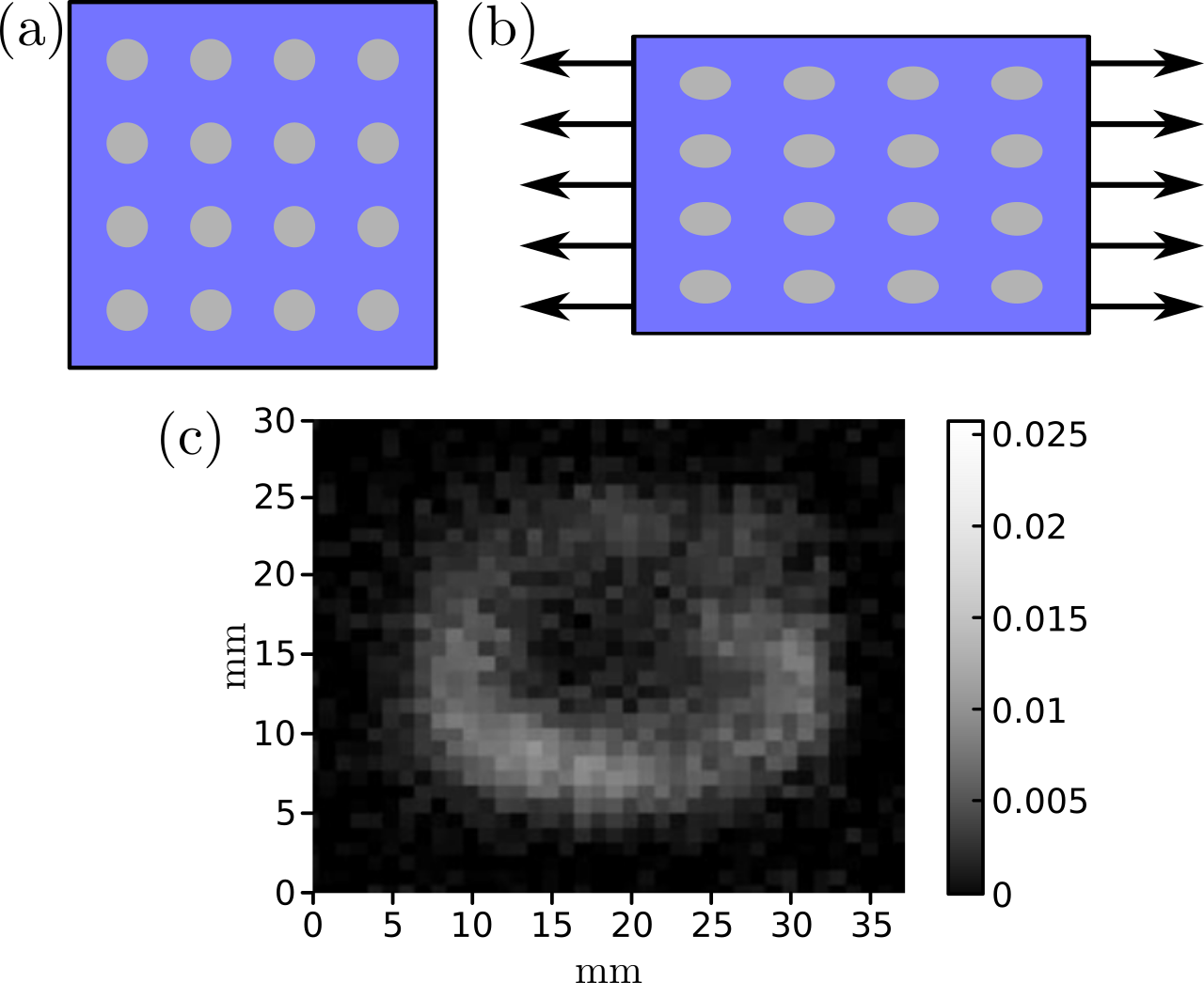
Figure 10: Schematic of a metamaterial exhibiting terahertz frequency strain birefringence using reversible, elastic meta-atoms in unstressed (a) and stretched (b) situations. (c) Spatial map of the photoelastic strain measured for a terahertz metamaterial. The stretched sample was placed between crossed polarizers and raster scanned through a narrow terahertz beam at the resonance frequency that was detected by a single broadband detector. The grayscale represents the unnormalized cross polarimetric signal indicating the regions experiencing the greatest strain.

Another challenge in applying the techniques described in §5 to more realistic situations, is to allow their application to particles that are non-circular or cohesive, such as commonly arise in geophysical and industrial contexts. For circular particles with cohesion (i.e. electrostatic interactions, liquid bridges, chemical bonds), the inverse methods described in §5.3 likely still apply. However, the key technical challenge for non-circular particles is that the inverse problem is only well-specified for the case of circular particles, where the trivial surface geometry (all tangential forces are torques, all normal are central) dramatically simplify the formulation of the inverse solution to Eq. (3). New mathematical solutions are required to created a more general formulation to apply to particles of arbitrary shape.

Another persistent challenge is to move from quasi-static experiments to fully dynamic. Previously, this was accomplished by performing semi-quantitative force analysis, as described by the $G^{2}$ method in §5.2. Recently, advances in high-speed imaging have made it possible to record images with sufficient brightness and resolution to perform photoelastic analysis on continuously-avalanching flows, and thereby obtain vector contact forces via adaptations of the methods in §5.3 Thomas and Vriend (2019). This process is enabled by measuring the particle positions directly from a single movie of photoelastic images, in order to capture as much light as possible. Furthermore, because the particles are accelerating, it is not possible to use particle-scale force-balance as a constraint in determining the vector contact forces.

Finally, computational advances in inverting the photoelastic images would improve the applicability of photoelastimetry to all of the problems presented here. Better algorithms for avoiding unintended-minima and the ability to simultaneously solve for all vector contact forces in the system (a massive set of constraints) would improve the reliability of these methods.

It is our hope that the recent proliferation of publications of photoelastimetric techniques in open formats Zadeh et al. (2019); Lantsoght and Docquier (2018); Kollmer (2018) will spur development in all of these new directions.

References

- Zadeh et al. [2019] A. A. Zadeh, J. Barés, T. Brzinski, K. E. Daniels, J. Dijksman, N. Docqiuer, H. Everitt, J. Kollmer, O. Lantsoght, D. Wang, M. Workamp, Y. Zhao, and H. Zheng. Photoelastic methods wiki. https://git-xen.lmgc.univ-montp2.fr/PhotoElasticity/Main/wikis/home, 2019.
- Frocht [1969] M. M. Frocht. Photoelasticity: the selected scientific papers of MM Frocht, volume 2. Pergamon, 1969.
- Cloud [1995] G. Cloud. Photoelasticity, page 55–56. Cambridge University Press, 1995.
- Daniels et al. [2017] K. E. Daniels, J. E. Kollmer, and J. G. Puckett. Photoelastic force measurements in granular materials. Review of Scientific Instruments, 88(5):051808, 2017.
- Cox et al. [2016] M. Cox, D. Wang, J. Barés, and R. P. Behringer. Self-organized magnetic particles to tune the mechanical behavior of a granular system. Europhysics Letters, 115(6):64003, 2016.
- Wakabayashi [1950] T. Wakabayashi. Photo-elastic method for determination of stress in powdered mass. Journal of the Physical Society of Japan, 5(5):383–385, 1950.
- Dantu [1957] P. Dantu. Proceedings of the 4th international conference on soil mechanics and foundations engineering. 1957.
- A and Josselin [1972] Drescher A and G. De Jong De Josselin. Photoelastic verification of a mechanical model for the flow of a granular material. Journal of the Mechanics and Physics of Solids, 20(5):337–340, 1972.
- Liu et al. [1995] C. H. Liu, S. R. Nagel, D. A. Schecter, S. N. Coppersmith, S. Majumdar, O Narayan, and T. A. Witten. Force fluctuations in bead packs. Science, 269(5223):513–515, 1995.
- Howell et al. [1999] D. Howell, R. P. Behringer, and C. Veje. Stress fluctuations in a 2d granular couette experiment: a continuous transition. Physical Review Letters, 82(26):5241, 1999.
- Majmudar and Behringer [2005] T. S. Majmudar and R. P. Behringer. Contact force measurements and stress-induced anisotropy in granular materials. Nature, 435(7045):1079, 2005.
- Amon et al. [2017] A. Amon, P. Born, K. E. Daniels, J. A. Dijksman, K. Huang, D. Parker, M. Schröter, R. Stannarius, and A. Wierschem. Preface: Focus on imaging methods in granular physics, 2017.
- Barés et al. [2017a] J. Barés, S. Mora, J.-Y. Delenne, and T. Fourcaud. Experimental observations of root growth in a controlled photoelastic granular material. In EPJ Web of Conferences, volume 140, page 14008. EDP Sciences, 2017a.
- Kollmer [2018] J. E. Kollmer. Photoelastic grain solver (pegs). https://github.com/jekollmer/PEGS, 2018.
- Lantsoght and Docquier [2018] O. Lantsoght and N. Docquier. Photoelastic grain solver with pyhton (pegspy). https://git.immc.ucl.ac.be/olantsoght/pegs_py, 2018.
- Barés et al. [2017b] J. Barés, D. Wang, D. Wang, T. Bertrand, C. S. O’Hern, and Robert P R. P. Behringer. Local and global avalanches in a two-dimensional sheared granular medium. Physical Review E, 96(5):052902, 2017b.
- Zadeh et al. [2018] A. Abed Zadeh, J. Barés, J. Socolar, and R. P. Behringer. Seismicity in sheared granular matter. arXiv preprint arXiv:1810.12243, 2018.
- Geng et al. [2001] Junfei Geng, D Howell, E Longhi, RP Behringer, G Reydellet, L Vanel, E Clément, and S Luding. Footprints in sand: the response of a granular material to local perturbations. Physical Review Letters, 87(3):035506, 2001.
- Zhang et al. [2010] J. Zhang, T. S. Majmudar, A. Tordesillas, and R. P. Behringer. Statistical properties of a 2d granular material subjected to cyclic shear. Granular Matter, 12(2):159–172, 2010.
- Majmudar et al. [2007] T. S. Majmudar, M. Sperl, S. Luding, and R. P. Behringer. Jamming transition in granular systems. Physical review letters, 98(5):058001, 2007.
- Bi et al. [2011] Dapeng Bi, Jie Zhang, Bulbul Chakraborty, and R. P. Behringer. Jamming by shear. Nature, 480:355–358, 2011.
- Ren et al. [2013] J. Ren, J. A. Dijksman, and R. P. Behringer. Reynolds pressure and relaxation in a sheared granular system. Physical review letters, 110(1):018302, 2013.
- Zheng et al. [2014] Hu Zheng, Joshua A Dijksman, and Robert P Behringer. Shear jamming in granular experiments without basal friction. EPL (Europhysics Letters), 107(3):34005, 2014.
- Wang et al. [2018] Dong Wang, Jie Ren, Joshua A. Dijksman, Hu Zheng, and Robert P. Behringer. Microscopic origins of shear jamming for 2d frictional grains. Phys. Rev. Lett., 120:208004, 2018.
- Clark et al. [2012] A. H. Clark, L. Kondic, and R. P. Behringer. Particle scale dynamics in granular impact. Physical review letters, 109(23):238302, 2012.
- Lim et al. [2017] M. X. Lim, J. Barés, H. Zheng, and R. P. Behringer. Force and mass dynamics in non-newtonian suspensions. Physical review letters, 119(18):184501, 2017.
- Zheng et al. [2018] Hu Zheng, Dong Wang, David Z. Chen, Meimei Wang, and Robert P. Behringer. Intruder friction effects on granular impact dynamics. Phys. Rev. E, 98:032904, 2018.
- Zuriguel and Mullin [2008] I Zuriguel and T Mullin. The role of particle shape on the stress distribution in a sandpile. Proceedings of the Royal Society A: Mathematical, Physical and Engineering Sciences, 464(2089):99–116, 2008.
- Lherminier et al. [2014] S Lherminier, R Planet, G Simon, L Vanel, and O Ramos. Revealing the Structure of a Granular Medium through Ballistic Sound Propagation. Physical Review Letters, 113(9):098001, 2014.
- Shukla [1991] Arun Shukla. Dynamic photoelastic studies of wave propagation in granular media. Optics and Lasers in Engineering, 14(3):165–184, 1991.
- Owens and Daniels [2011] Eli T. Owens and Karen E. Daniels. Sound propagation and force chains in granular materials. Europhysics Letters, 94(5):54005, 2011.
- Huillard et al. [2011] Guillaume Huillard, Xavier Noblin, and Jean Rajchenbach. Propagation of acoustic waves in a one-dimensional array of noncohesive cylinders. Physical Review E, 84:016602, 2011.
- Puckett and Daniels [2013] J. G. Puckett and K. E. Daniels. Equilibrating temperaturelike variables in jammed granular subsystems. Physical Review Letters, 110(5):058001, 2013.
- Bililign et al. [2019] Ephraim S. Bililign, Jonathan E. Kollmer, and Karen E. Daniels. Protocol Dependence and State Variables in the Force-Moment Ensemble. Physical Review Letters, 122(3), 2019.
- Kollmer and Daniels [2018] J. E. Kollmer and K. E. Daniels. Betweenness centrality as predictor for forces in granular packings. Soft Matter, 2018.
- Coulais et al. [2014] C Coulais, A Seguin, and O Dauchot. Shear Modulus and Dilatancy Softening in Granular Packings above Jamming. Physical Review Letters, 113(19):198001, 2014.
- Iikawa et al. [2016] N Iikawa, M M Bandi, and H Katsuragi. Sensitivity of Granular Force Chain Orientation to Disorder-Induced Metastable Relaxation. Physical Review Letters, 116(12):128001, 2016.
- Mahabadi and Jang [2017] N Mahabadi and J Jang. The impact of fluid flow on force chains in granular media. Applied Physics Letters, 110(4):041907, 2017.
- Wendell et al. [2012] D. M. Wendell, K. Luginbuhl, J. Guerrero, and A. E. Hosoi. Experimental investigation of plant root growth through granular substrates. Experimental Mechanics, 52(7):945–949, 2012.
- Kolb et al. [2012] E Kolb, C Hartmann, and P Genet. Radial force development during root growth measured by photoelasticity. Plant Soil, 360:19–35, 2012.
- Daniels and Hayman [2008] Karen E Daniels and Nicholas W Hayman. Force chains in seismogenic faults visualized with photoelastic granular shear experiments. Journal of Geophysical Research, 113(B11):B11411, 2008.
- Hayman et al. [2011] Nicholas W. Hayman, Lucie Ducloué, Kate L. Foco, and Karen E. Daniels. Granular Controls on Periodicity of Stick-Slip Events: Kinematics and Force-Chains in an Experimental Fault. Pure and Applied Geophysics, 168(12):2239–2257, 2011.
- Geller et al. [2015] Drew A. Geller, Robert E. Ecke, Karin A. Dahmen, and Scott Backhaus. Stick-slip behavior in a continuum-granular experiment. Physical Review E, 92(6):060201, December 2015.
- Lherminier et al. [2019] S. Lherminier, R. Planet, V. Levy dit Vehel, G. Simon, L. Vanel, K. J. Maloy, and O. Ramos. Continuously sheared granular matter reproduces in detail seismicity laws. arXiv:1901.06735, January 2019.
- Trushant S Majmudar [2006] Trushant S Majmudar. Experimental Studies of Two-Dimensional Granular Systems Using Grain-Scale Contact Force Measurements. PhD thesis, Duke University, 2006.
- [46] Precision urethane pads. http://www.precisionurethane.com/polyurethane-pads.html.
- [47] Clear flex™, castable urethane from smooth-on. https://www.smooth-on.com/product-line/clear-flex/.
- [48] Vishay pads. http://www.vishaypg.com/micro-measurements/photo-stress-plus.
- Wang [2018] D. Wang. Response of Granular Materials to Shear: Origins of Shear Jamming, Particle Dynamics, and Effects of Particle Properties. PhD thesis, Duke University, 2018.
- [50] Mold star™, castable silicone from smooth-on. https://www.smooth-on.com/product-line/mold-star/.
- [51] So strong™, dye for urethane from smooth-on. https://www.smooth-on.com/product-line/strong/.
- Kilcast et al. [1984] D. Kilcast, M. M. Boyar, and J. B. Hudson. Gelatin photoelasticity: A new technique for measuring stress distributions in gels during penetration testing. Journal of Food Science, 49(2):654–655, 1984.
- Workamp et al. [2017] M. Workamp, S. Alaie, and J. A. Dijksman. What is fluidity? designing an experimental system to probe stress and velocity fluctuations in flowing suspensions. In EPJ Web of Conferences, volume 140, page 03020. EDP Sciences, 2017.
- Tomlinson and Taylor [2015] R. A Tomlinson and Z. A. Taylor. Photoelastic materials and methods for tissue biomechanics applications. Optical Engineering, 54(8):081208, 2015.
- Damink et al. [1995] L. H. O. Damink, P. J. Dijkstra, M. J. A. Van Luyn, P. B. Van Wachem, P. Nieuwenhuis, and J. Feijen. Glutaraldehyde as a crosslinking agent for collagen-based biomaterials. Journal of materials science: materials in medicine, 6(8):460–472, 1995.
- Workamp et al. [2016] M. Workamp, S. Alaie, and J. A. Dijksman. Coaxial air flow device for the production of millimeter-sized spherical hydrogel particles. Review of Scientific Instruments, 87(12):125113, 2016.
- Lherminier et al. [2016] S. Lherminier, R. Planet, G. Simon, M. Måløy, L. Vanel, and O. Ramos. A granular experiment approach to earthquakes. Revista Cubana de Física, 33(1):55–58, 2016.
- [58] Veroclear™, printable transparent photoelastic material from smooth-on. https://www.stratasys.com/materials/search/veroclear.
- Wang et al. [2017] L. Wang, Y. Ju, H. Xie, G. Ma, L. Mao, and K. He. The mechanical and photoelastic properties of 3d printable stress-visualized materials. Scientific Reports, 7(1):10918, 2017.
- [60] Polarization, a company which sells polarizers and quater-waves plates by the foot. http://www.polarization.com/polarshop/.
- Zhao et al. [2017] Y. Zhao, J. Barés, H. Zheng, and R. P. Behringer. Tuning strain of granular matter by basal assisted couette shear. In EPJ Web of Conferences, volume 140, page 03049. EDP Sciences, 2017.
- Shattuck [2015] M D Shattuck. Experimental Techniques. In Scott V. Franklin and Mark D. Shattuck, editors, Handbook of Granular Materials. CRC Press, 2015.
- Peng et al. [2007] T. Peng, A. Balijepalli, S. K. Gupta, and T. LeBrun. Algorithms for on-line monitoring of micro spheres in an optical tweezers-based assembly cell. J. Comput. Inf. Sci. Eng., 79:330–338, 2007.
- Crocker and Grier [1996] J. C. Crocker and D. G. Grier. Methods of digital video microscopy for colloidal studies. Journal of colloid and interface science, 179(1):298–310, 1996.
- [65] D. Blair and E. Dufresne. Matlab particle tracking code repository. http://site.physics.georgetown.edu/matlab/.
- Willert and Gharib [1991] C. E. Willert and M. Gharib. Digital particle image velocimetry. Experiments in fluids, 10(4):181–193, 1991.
- Landau and Lifshitz [1986] Lev D Landau and EM Lifshitz. Theory of elasticity, vol. 7. Course of Theoretical Physics, 3:109, 1986.
- Zhao et al. [2019] Yiqiu Zhao, Hu Zheng, Dong Wang, Meimei Wang, and Robert P Behringer. Particle scale force sensor based on intensity gradient method in granular photoelastic experiments. New Journal of Physics, in press, 2019. URL https://doi.org/10.1088/1367-2630/ab05e7.
- Majmudar [2006] Trushant Suresh Majmudar. Experimental studies of two-dimensional granular systems using grain-scale contact force measurements (Doctoral Dissertation). Duke University, 2006.
- Farhadi and Behringer [2014] Somayeh Farhadi and Robert P Behringer. Dynamics of sheared ellipses and circular disks: effects of particle shape. Physical review letters, 112(14):148301, 2014.
- Farhadi et al. [2015] Somayeh Farhadi, Alex Z Zhu, and Robert P Behringer. Stress relaxation for granular materials near jamming under cyclic compression. Physical review letters, 115(18):188001, 2015.
- Iikawa et al. [2015] Naoki Iikawa, Mahesh M. Bandi, and Hiroaki Katsuragi. Structural evolution of a granular pack under manual tapping. Journal of the Physical Society of Japan, 84(9):094401, 2015. doi: 10.7566/JPSJ.84.094401. URL https://doi.org/10.7566/JPSJ.84.094401.
- Lantsoght [2019] O. Lantsoght. Couplage entre dynamique multicorps et méthode des éléments discrets : modélisation et expérimentation. phdthesis, Université Catholique de Louvain, 2019.
- Timoshenko and Goodier [1970] S. Timoshenko and J. N. Goodier. Theory of Elasticity. McGraw-Hill, 3rd ed edition, 1970.
- Wang et al. [2004] Z. Wang, A. C. Bovik, H. R. Sheikh, and E. P. Simoncelli. Image quality assessment: from error visibility to structural similarity. IEEE Transactions on Image Processing, 13(4):600–612, 2004.
- Yu et al. [2014] Peidong Yu, Stefan Frank-Richter, Alexander Börngen, and Matthias Sperl. Monitoring three-dimensional packings in microgravity. Granular Matter, 16(2):165–173, April 2014.
- Mahon et al. [2006] R. J. Mahon, J. A. Murphy, and W. Lanigan. Digital holography at millimetre wavelengths. Optics Communications, 260(2):469–473, 2006.
- Heimbeck et al. [2011] M. S. Heimbeck, M. K. Kim, D. A. Gregory, and H. O. Everitt. Terahertz digital holography using angular spectrum and dual wavelength reconstruction methods. Optics Express, 19(10):9192–9200, 2011.
- Everitt et al. [2019] H. O. Everitt, T. Tyler, B. D. Caraway, C. M. Bingham, A. Llopis, M. S. Heimbeck, W. J. Padilla, D. R. Smith, and N. M. Jokerst. Strain sensing with metamaterial composites. Submitted to Advanced Optical Materials, 2019.
- Thomas and Vriend [2019] A. L. Thomas and N. M. Vriend. Photoelastic study of dense granular free-surface flows. preprint, 2019.