Lattice Boltzmann Models for Micro-tomographic Pore-spaces

Abstract

The lattice Boltzmann method (LBM) is a popular numerical framework to investigate single and multiphase flow though porous media. For estimation of absolute permeability based on micro-tomographic images of the porous medium, the single-relaxation time (SRT) collision model is the most widely-used, although the multiple-relaxation-time (MRT) collision model also has recently acquired wider usage, especially for industrial applications. However, the SRT collision model and a sub-optimal choice of the MRT collision parameters can both lead to permeability predictions that depend on the relaxation time, $\tau$. This parametric dependence is nonphysical for Stokes flow in porous media and also leads to much larger number of iterations required for convergence. In this paper, we performed a systematic numerical evaluation of the different sets of relaxation parameters in the D3Q19-MRT model for modeling Stokes flow in 3-D microtomographic pore-spaces using the bounceback scheme. These sets of parameters are evaluated from the point of view of accuracy, convergence rate, and an ability to generate parameter-independent permeability solutions. Instead of tuning all six independent relaxation rates that are available in the MRT model, the sets that were analyzed have relaxation rates that depend on one or two independent parameters, namely $\tau$ and $\Lambda$. We tested elementary porous media at different image resolutions and a random packing of spheres at relatively high resolution. We observe that sets of certain specific relaxation parameters (Sets B, D, or E as listed in Table 2), and $\tau$ in the range $\tau\in[1.0,1.3]$ can result in best overall accuracy, convergence rate, and parameter-independent permeability predictions.

1 Introduction

Flow and transport in reservoir rocks and other porous media are strongly dependent on the properties of the pore-space, such as the geometry, distribution, and connectivity. Laboratory-based core analysis are the main tools for studying and quantifying rock properties for practical and scientific applications. Over the past decade, high-resolution, three-dimensional (3-D), X-ray microtomography imaging and processing capabilities have become widely available [34]. These advances have enabled one to obtain a 3-D reconstructed pore-space domain which serve as an input for the direct numerical simulation of the underlying fluid and transport processes. In this approach, also commonly called Digital Rock Physics (DRP) in the oil and gas industry, transport properties of rocks, such as absolute (intrinsic) permeability, relative permeability, dispersivity, formation factor, etc., are computed on geometries constructed from 3-D microtomographic images [2]. In this study, we focus on the permeability of a porous medium for single phase flow for Newtonian fluids.

For direct numerical simulation of flow in microtomographic pores-spaces, the lattice Boltzmann method (LBM) has emerged as a method of choice [9, 11, 18, 24, 25, 31, 37]. After imaging, a cubic voxel in the 3-D image is segmented such that each voxel is labeled as either a fluid or a solid. The resulting fluid-solid interface, henceforth called the solid boundary, is inherently rough and stair-step patterned, and which represents the surface roughness of the medium at a length scale comparable to the resolution of the image. Since the pore-space is already discretized via the voxels, the segmented binary image lends itself immediately to numerical simulations via the LBM without the additional step of pre-processing, such as surface extraction and volume meshing that is needed in traditional CFD. Pre-processing techniques, especially for tortuous porous geometries, are tedious and therefore difficult to scale and automate. Besides this advantage, there are other well-recognized benefits of the LBM approach, such as the localized nature of the algorithm that enables parallelization and good performance scalability, both essential features for rapid and routine analysis of very large $(>1024^{3})$ images with minimal user interface. One of the main challenges, however, is the is the accuracy of the predictions.

The accuracy of the permeability predictions on pore-spaces obtained from imaging depend strongly on the the sampling rate (minimum voxel size) and the thresholding values used for the segmentation procedure [4]. For a segmented image of a given voxel resolution, within the LBM framework, the overall accuracy of the permeability predictions depends on boundary schemes for the solid boundary, inlet and outlet boundary conditions, simulation parameters, and techniques used to initiate the flow within the porous sample (body-force driven or pressure gradient). Numerical artifacts arising due to each the above factors contribute to a varying degree to the overall inaccuracy.

The numerical technique used to enforce a zero (no-slip) velocity condition on the solid boundary using the so-called bounceback (BB) scheme is one of the largest sources of errors. Bounceback boundaries are particularly simple to implement and have played a major role in making LBM popular. The simplicity lies in that one simply needs a particular voxel to be labeled as a solid (obstacle) and no additional numerical procedure is required. Although robust and mass conserving, a well-known defect of the bounceback scheme is the fact that, when used conjunction with the single-relaxation-time (SRT) collision model, the exact physical location of the solid boundary depends on the relaxation time $\tau$, a LBM parameter that numerically sets the kinematic viscosity, $\nu$ of the fluid via the relation $\nu=(\tau-0.5)\delta t/3$. This spatial error is proportional to $(\tau-\delta t/2{}^{2})$ [6, 12, 14]. As an example, for Poiseuille flow in a straight channel, the theoretical permeability value is $k=H^{2}/12,$ while the error in the permeability obtained numerically with BB-SRT method is equal to $(4\nu^{2}-\delta t/12)$ [14]. Because $\tau$ controls both the kinematic viscosity and solution accuracy, the computed permeability is said to be viscosity-dependent. Physically this means that the effective pore size is a function of viscosity, a clear violation of physical behavior. In addition to the nonphysical nature of the $k-\nu$ dependence, there are several consequences of this parametric dependence of practical import. Firstly, since the non-dimensional solutions of Stokes flow do not depend on viscosity, performing simulations with BB-SRT scheme with different values of $\tau$ will yield different permeability values of the porous media. Secondly, since the LBM is not as efficient for steady flows, a practical method to improve convergence towards the steady state is to use large values of $\tau$ or $(\nu)$. However, for $\tau\gg 1,$ the numerical errors increase quadratically and therefore not advisable especially for porous media flow where since the surface to volume ratio is large. Such parametric dependence of permeability leads to subjectivity or operator bias, much similar to the subjectivity arising due to the thresholding values used in the image segmentation step- a challenge recognized in the DRP community [4, 34].

The first and most obvious method to improve to improve the prediction accuracy and reduce $k-\nu$ dependence, is to increase the voxel resolution. This approach is not always practical due to constraints of the imaging equipment. The second method is to employ more accurate wall-boundary schemes, such as the multi-reflection scheme, spatial-interpolation based schemes, and other second-order accurate interpolation-based techniques for curved boundaries [14, 3, 35]. Although these provide improvement in accuracy, these schemes require that the location of the solid boundary surface be known in reference to the underlying voxel grid/lattice [1, 8, 29, 23]. The location of the boundary surface is quantified by the so-called sub-grid or wall distance, usually denoted as $q_{i}(\boldsymbol{x}),$ which represents the projected distance from the boundary voxel to the solid boundary surface along the lattice links. Wall distances can be evaluated relatively easily for analytic surfaces, such as spheres, cylinders, and sphere packings, but can become tedious for microtomographic images due to the additional pre-processing steps, such as reconstructing a boundary surface using a smoothing (iso-surface extraction) operation based on the marching-cubes algorithm [23, 36, 37]. With the projected imminent increase in imaging capabilities, with image datasets as large as $2000^{3}$ becoming available, the bounceback scheme remains an utilitarian option for microtomographic image based pore-spaces, especially when large numbers of samples have to analyzed rapidly from various regions of the reservoir/wells. It should also be noted that, with the SRT model, the permeability depends on the viscosity even if more accurate boundary schemes are employed [6].

Therefore, given an a priori choice of the bounceback scheme, the third option to improve the accuracy and produce viscosity-independent permeability is to use more complex collision models, such as the multi-relaxation-time (MRT) [5, 20, 22] or two-relaxation-time (TRT) collision models [6, 13, 15]. The essential idea of these collision models is that, unlike the SRT model, the MRT/TRT models provide additional free relaxation parameters - six in the case of MRT and two in case of TRT-that can be tuned to obtain more accurate or stable solutions [22]. When the MRT/TRT collision models are applied with the bounceback condition, they provide a mechanism to correct for the boundary error (and obtain viscosity-independent results) by tuning the relaxation parameters, the choice of which is essentially empirical for non-trivial porous media, such as reservoir rocks. However, it should be noted that the mere application of MRT/TRT model, instead of the SRT model, may not result in viscosity-independent results unless the relaxation parameters are carefully chosen. In fact, a sub-optimal choice of the MRT relaxation parameters does not actually produce to viscosity-independent results as can be seen several recent works [7, 28, 31]. Therefore, from an application-oriented user perspective, the question remains: which set of MRT relaxation parameters would provide the most accurate and viscosity-independent (or parameter-independent) permeability prediction for a certain class of porous media/rocks?

To address this concern, in this paper, we perform a systematic numerical evaluation of the different sets of relaxation parameters within the MRT framework for modeling Stokes flow in microtomographic pore-spaces. These sets of relaxation parameters are evaluated from the point of view of accuracy and an ability to generate viscosity-independent solutions. For this purpose, we study two elementary porous media (channels with circular and triangular cross sections) and a high-resolution, random, dense packing of identical spheres, a first-order approximation for sandstone rock. The rest of the paper is organized as follows. In Sec. 2, we describe the essential details of the LBM collision models, detail the various parameterization choices for the MRT model, and briefly describe the boundary conditions used in this study. In Sec. 3, we discuss the result obtained from the numerical experimentation on various porous geometries and in Sec. 4, we present our conclusions.

2 The Lattice Boltzmann Equation

Compared to the classical approach of directly solving the Navier-Stokes equation to model hydrodynamics, the lattice Boltzmann equation (LBE) is based on kinetic theory and the Boltzmann equation [17, 19, 21]. The LBE solves the discrete Boltzmann equation on a space $\boldsymbol{x}$ that is discretely represented as a lattice $\delta x\mathbb{Z}^{d}$ in d dimensions with a lattice constant $\delta x$, and where the time $t$ is discretized with a constant time step-size $\delta t$, i.e., $t_{n}\in\delta t\mathbb{N}_{0}$ with $\mathbb{N}_{0}={0,1,...}$. The continuous velocity-space of the Boltzmann equation is approximated by a set of discrete velocities $\mathbb{V}\equiv\{\boldsymbol{c}_{i}|i=0,1,\cdots,b\}$ that it is symmetric, $\mathbb{V}=-\mathbb{V}$ and $c_{0}=\boldsymbol{0}$ [22]. In the LBE, the phase-space $(\boldsymbol{x}-\boldsymbol{c})$ and the time discretization are coupled such that for any $\boldsymbol{c}_{i}\in\mathbb{V}$, if $\boldsymbol{x}$ is a node, then $\boldsymbol{x}+\delta t\boldsymbol{c}_{i}$ is also a node of the lattice. Such a lattice is usually denoted as DdQq, where $d$ is number of space dimension and $q=b+1$ represents the total number of discrete velocities in the set. On such a discrete system, the evolution of the distribution functions $f_{i}(\boldsymbol{x})$ is given by:

$$f_{i}(\boldsymbol{x}+\boldsymbol{c}_{i}\delta t,t+\delta t)=f_{i}(\boldsymbol{x},t)+C_{i}\delta t+F_{i}\delta t$$ (1)

where $f_{i},C_{i},$ and $F_{i}$ are q-dimensional (column) vectors. Eqn. 1 consists of three distinct terms: the term on the left-hand side describes the free flight (streaming) of the distributions from one computational (lattice) node to the other according to their discrete velocities $\boldsymbol{c}_{i},$ $C_{i}$ describes the local changes to distributions due to inter-particle collisions, and $F_{i}$ describes the changes (sources) of momentum density due to external body forces. The most widely used lattice structure for isothermal hydrodynamics is the D2Q9 lattice in 2-D and D3Q19 and D3Q15 lattices in 3-D. In this work we use the D3Q19 lattice.

2.1 Collision Models

The most widely used collision model is the so-called Bhatnagar-Gross-Krook (BGK) model, which assumes that all the distributions relax to a local equilibrium value at a single rate characterized by a relaxation time $\tau,$

$$\boldsymbol{C}^{BGK}\equiv-\frac{1}{\tau}\left[\boldsymbol{f}(\boldsymbol{x},t)-\boldsymbol{f}^{(eq)}(\boldsymbol{x},t)\right]$$ (2)

Since only one relaxation time is used, the BGK model is also termed the single-relaxation-time (SRT) model. The local equilibrium is given by the Maxwell-Boltzmann distribution, which is itself a function of the local hydrodynamic variables, $f_{i}^{eq}=f_{i}^{eq}(\rho,\boldsymbol{u})$. The functional form of the equilibrium distributions is obtained by expanding the Maxwell-Boltzmann distribution up to second-order in local flow velocity:

$$f_{i}^{(eq)}(\boldsymbol{x},t)=w_{i}\rho(\boldsymbol{x},t)\bigg{(}1+\frac{(\boldsymbol{c}_{i}\cdot\boldsymbol{u})}{c_{s}^{2}}+\frac{(\boldsymbol{c}_{i}\cdot\boldsymbol{u})^{2}}{2c_{s}^{4}}-\frac{(\boldsymbol{u}\cdot\boldsymbol{u})}{2c_{s}^{2}}\bigg{)}$$ (3)

The relaxation time is related to the fluid’s kinematic viscosity via $\nu=c_{s}^{2}(\tau-0.5)\delta t=c_{s}^{2}(\frac{1}{s_{\nu}}-0.5)\delta t$, where $s_{\nu}=\frac{1}{\tau}$ is the relaxation rate. Note that the terms ’relaxation rate’ and ’relaxation parameters’ (in case of MRT/TRT models) are used interchangeably.

2.1.1 MRT Collision Model

In contrast to the SRT model where all distributions relax at a single rate, in the multiple-relaxation-time (MRT) model, the collision process occurs in the moment space, where each moment of the distribution can relax towards the local equilibrium at its own independent relaxation rate. The MRT collision model is based on the generalized lattice Boltzmann equation (GLBE) method, where while the streaming of the populations occurs in the velocity-space, the collision occurs in the moment-space, which is spanned by the orthogonal eigenvectors basis of the collision operator. The MRT collision operator is expressed as:

$$\boldsymbol{C}^{MRT}\equiv-\mathbf{M}^{-1}S\mathbf{M}[{\rm\boldsymbol{f}}-{\rm\boldsymbol{f}^{eq}}]=-\mathbf{M}^{-1}S[{\rm\boldsymbol{m}}-{\rm\boldsymbol{m}^{eq}}]$$ (4)

where $\mathbf{M}$ is a $q\times q$ matrix that linearly transforms the $q$-dimensional vector of distribution function ${\rm\boldsymbol{f}},$ from the velocity-space to a $q$-dimensional vector ${\rm\boldsymbol{m}},$ in the moment-space:

$${\rm\boldsymbol{m}}=\boldsymbol{{\rm M}}\cdot{\rm\boldsymbol{f}}\quad\boldsymbol{{\rm f}}={\rm\boldsymbol{M}^{-1}}\cdot\boldsymbol{{\rm m}}$$ (5)

and the LBE-MRT equation is:

$$\boldsymbol{{\rm f}}(\boldsymbol{x}+\boldsymbol{c}_{i}\delta t,t+\delta t)={\rm\boldsymbol{f}}(\boldsymbol{x},t)-\mathbf{M}^{-1}S[{\rm\boldsymbol{m}}-{\rm\boldsymbol{m}^{eq}}]\delta t$$ (6)

The rows of the transformation matrix $\mathbf{M},$ for the D3Q19 model consist of 19 orthogonal basis vectors, can be found in [5]. The corresponding nineteen moments $\boldsymbol{m}$ of the distributions are arranged in the following sequence:

$$\mathbf{m}\equiv(\rho,e,\epsilon,j_{x},q_{x},j_{y},q_{y},j_{z},q_{z},3p_{xx},3\pi_{xx},p_{ww},\pi_{ww},p_{xy},p_{yz},p_{xz},m_{x},m_{y},m_{z}).$$

Among the 19 moments, the $0$th-order moment corresponds to mass density $m_{0}=\rho$ and the three 1st-order moments correspond to momentum $m_{3,5,7}=j_{x,y,z}=\rho_{0}u_{x,y,z}.$ The six $2$nd-order moments: $m_{1}=e,\,m_{9}=3p_{xx},\,m_{11}=p_{ww}=p_{yy}-p_{zz}$ and $m_{13,14,15}=p_{xy,yz,xz}$ correspond to part of the kinetic energy, the diagonal, and off-diagonal elements of the viscous stress tensor, respectively. Moments higher than second-order are called as higher-order moments (also ghost moments) and they do not have a clear physical connection to incompressible Navier-Stokes limit of hydrodynamics, but are characterized by their dependence on the gradient of the conserved moments. These higher-order moments are the six 3rd-order moments $m_{4,6,8}=q_{x,y,z},\,m_{16,17,18}=m_{x,y,z}$ and three 4th-order moments $m_{2}=\epsilon,\,m_{10}=3\pi_{xx},\,m_{12}=\pi_{ww}$. We refer to Table 1 that summarizes these relations.

The equilibrium moments are $m_{0}=m_{0}^{eq}=\rho=\sum_{i}f_{i}$ and $m_{3,5,7}=m_{3,5,7}^{eq}=j_{x,y,z}=\sum_{i}\boldsymbol{c}_{i}f_{i}$ since density and momentum are conserved during the collision process. The local equilibrium moments for the non-conserved moments, which are themselves functions of the conserved moments, are given as [5, 29]:

$$m_{1}^{eq} =m_{e}^{eq}=11\rho+\frac{19}{\rho_{0}}(j_{x}^{2}+j_{y}^{2}+j_{z}^{2})$$

$$m_{2}^{eq} =m_{\epsilon}^{eq}=3\rho-\frac{11}{2\rho_{0}}(j_{x}^{2}+j_{y}^{2}+j_{z}^{2})$$

$$m_{4}^{eq}=m_{q_{x}}^{eq} =-\frac{2}{3}j_{x},\quad m_{6}^{eq}=m_{q_{y}}^{eq}=-\frac{2}{3}j_{y},\quad m_{8}^{eq}=m_{q_{z}}^{eq}=-\frac{2}{3}j_{z}$$

$$m_{9}^{eq}=3p_{xx}^{eq}=\frac{1}{\rho_{0}}(j_{x}^{2}-j_{y}^{2}-j_{z}^{2}), m_{11}^{eq}=p_{ww}=\frac{1}{\rho_{0}}(j_{y}^{2}-j_{z}^{2}),$$

$$m_{13}^{eq}=m_{p_{xy}}^{eq}=\frac{1}{\rho_{0}}j_{x}j_{y},\,\, m_{14}^{eq}=m_{p_{yz}}^{eq}=\frac{1}{\rho_{0}}j_{y}j_{z},\,\,m_{15}^{eq}=m_{p_{xz}}^{eq}=\frac{1}{\rho_{0}}j_{x}j_{z},$$ (7)

$$m_{10}^{eq}=m_{\pi_{xx}}^{eq}=-\frac{1}{2}p_{xx}^{eq}, \,\,m_{12}^{eq}=m_{\pi_{ww}}^{eq}=-\frac{1}{2}p_{ww}^{eq},$$

$$m_{16,17,18}^{eq}=m_{x,y,z}^{eq}=0$$

The relaxation rate matrix, $\mathbf{S}$, is a $q\times q$ diagonal matrix which consists of the relaxation rate of each corresponding moment, and which are the eigenvalues of the collision operator $\boldsymbol{\mathbf{M}^{-1}\mathbf{S}\mathbf{M}}$:

$$\mathbf{S} ={\rm diag}(0,s_{e},s_{\epsilon},0,s_{q},0,s_{q},0,s_{q},s_{\nu},s_{\pi},s_{\nu},s_{\pi},s_{\nu},s_{\nu},s_{\nu},s_{m},s_{m},s_{m})$$ (8)

The relaxation rates $\{s_{i}\}$ determine the transport coefficients in the system. The zero relaxation rates correspond to conserved moments $\{\rho,j_{x},j_{y},j_{z}\}$ while the non-zero relaxation rates are:

$$s_{1}=s_{e},\,\,s_{2}=s_{\epsilon},s_{4}=s_{6}=s_{8}=s_{q},$$

$$s_{10}=s_{12}=s_{\pi},\,\,s_{9}=s_{11}=s_{13}=s_{14}=s_{15}=s_{\nu}$$

$$s_{16}=s_{17}=s_{18}=s_{m}$$

The relaxation rate $s_{\nu}=\frac{1}{\tau}$ is related to the kinematic viscosity $\nu$ via $\nu=c_{s}^{2}\big{(}\frac{1}{s_{\nu}}-0.5\big{)}\delta t$ where for athermal hydrodynamics $c_{s}^{2}=c^{2}/3$, where $c\equiv\delta x/\delta t$. The remaining relaxation rates, $s_{e},s_{\epsilon},s_{q},s_{\pi},$ and $s_{m}$ can be set in the range $0<s_{i}<2$ in order to improve the accuracy and stability. Simplifications can be made for the equilibrium moments of the non-conserved quantities depending upon the flow at hand. For example, for Stokes flow, the non-linear terms in velocity can be ignored [29]. Another example is to set equilibrium moments of the higher order moments $m_{2,4,6,8,16,17,18}$ to zero since these do not have physical link to the incompressible Navier-Stokes behavior [1]. In this work, for the sake of generality, we use equilibrium moments as listed in Eqn 7.

The above discussion was valid for flows initiated by pressure gradients, or by shear, i.e. flows in the absence of external body forces. In the following, we describe the methodology to include external body forces, such as pressure gradient or gravity, within a MRT framework. Given an external body force density $\boldsymbol{F}=\rho_{0}\boldsymbol{a}$, where $\boldsymbol{a}$ is the acceleration due to applied force, the effects of this force can be incorporated in LBE by either modifying the equilibrium distribution function or by adding an explicit forcing or a source term, $F_{i}$ [17]. In this study, we employ the method suggested by Guo et al., where LBE-MRT equation with the force term is given as [16, 17]:

$$f_{i}(\boldsymbol{x}+\boldsymbol{c}_{i}\delta t,t+\delta t)=f_{i}(\boldsymbol{x},t)-M^{-1}\bigg{(}S[m_{i}-m_{i}^{eq}]-(I-\frac{1}{2}S)m_{i}^{F}\bigg{)}$$ (9)

where $I$ is the $q\times q$ identity matrix and $\boldsymbol{m}^{F}=m_{i}^{F}=M\cdot F_{i}$ are the moments of the forcing term $F_{i}=\left\{F_{0},F_{1},\cdots F_{b}\right\}^{T}$ which is related to the Cartesian components of body force $\boldsymbol{F}=\{F_{x},F_{y},F_{z}\}$ as:

$$F_{i}=w_{i}\left(\frac{\boldsymbol{c}_{i}-\boldsymbol{u}^{eq}}{c_{s}^{2}}+\frac{\left(\boldsymbol{c}_{i}\cdot\boldsymbol{u}^{eq}\right)\boldsymbol{c}_{i}}{c_{s}^{4}}\right)\cdot\boldsymbol{F}$$ (10)

Note that the velocity that is used to calculate the above forcing term and equilibrium moments in Eqn. 10 is shifted, i.e., $\rho\boldsymbol{u}^{eq}=\sum_{i}f_{i}\boldsymbol{c}_{i}+\frac{\rho_{o}\boldsymbol{a}\delta t}{2}$. The velocity field $u^{eq}$ also satisfies the Navier-Stokes equation up to the second-order in the Chapman-Enskog analysis. In practice, Eqn. 9, is implemented by first computing the post-collisional moments $m_{i}^{*}:$

$$m_{i}^{*}=m_{i}-s_{i}\left(m_{i}-m_{i}^{eq}\right)+\left(I-\frac{s_{i}\delta t}{2}\right)m_{i}^{F}$$ (11)

The post-collisional moments are then transformed back to velocity-space distributions $f_{i}^{*}$ via $f_{i}^{*}=M^{-1}\cdot m_{i}^{*},$ after which the regular streaming step is performed. The source moments, $m_{i}^{F}=M_{i}\cdot F_{i},$ can be pre-computed; in this work, however, we first compute $F_{i}$ per Eqn. 10, and then perform a matrix-vector multiplication $\boldsymbol{M}\cdot F_{i}$ to obtain $m_{i}^{F}$. A simpler way to include force is to approximate $F_{i}=3w_{i}\rho_{0}\frac{\boldsymbol{c}_{i}\cdot\boldsymbol{a}}{c^{2}}$ and add this term to RHS of Eqn. 6 [29].

Even-order non-conserved (symmetric) moments	2nd-order	$e$	$p_{xx}$	$p_{ww}$	$p_{xy}$	$p_{yz}$	$p_{xz}$
		$m_{1}$	$m_{9}$	$m_{11}$	$m_{13}$	$m_{14}$	$m_{15}$
	4th-order	$\epsilon$	$\pi_{xx}$	$\pi_{ww}$
		$m_{2}$	$m_{10}$	$m_{12}$
Odd-order non-conserved (anti-symmetric) moments	3rd-order	$q_{x}$	$q_{y}$	$q_{z}$	$m_{x}$	$m_{x}$	$m_{x}$
		$m_{4}$	$m_{6}$	$m_{8}$	$m_{16}$	$m_{17}$	$m_{18}$

Table 1: Non-conserved moments of the D3Q19 lattice

2.1.2 TRT Collision Model

The two-relaxation-time (TRT) model is a collision model that combines the improved accuracy and stability of the MRT model while preserving the simplicity of the SRT model. It was originally implemented within the MRT framework (by assuming only two independent relaxation parameters instead of six) [29], and later was developed independently. Unlike the MRT model, where the populations are projected on to a space spanned by the polynomial basis vectors, the TRT collision is based on a symmetry argument where the populations are projected on a pair of link basis vectors. For example, for a particular discrete velocity $\boldsymbol{c}_{i}$ there is a anti-symmetric velocity $\boldsymbol{c}_{\bar{i}}=-\boldsymbol{c}_{i}$, which is true for all velocities in a particular velocity set; $\{c_{i},c_{\bar{i}}\}$ constitute a pair of link basis vector. A projection on to link basis vectors leads to a decomposition of distributions into symmetric and the anti-symmetric parts, denoted by a $f_{i}^{+}$and $f_{i}^{-},$ respectively, and which can be defined as [19]:

$$f_{i}^{+} \equiv\frac{f_{i}+f_{\bar{i}}}{2},\qquad f_{i}^{-}\equiv\frac{f_{i}-f_{\bar{i}}}{2}$$ (12)

$$f_{0}^{+}=f_{0},\quad f_{0}^{-}=0$$ (13)

The symmetric and anti-symmetric part of the equilibrium distributions $f_{i}^{eq+}$ and $f_{i}^{eq-}$, respectively, are defined similarly. Given this decomposition, the TRT collision model can be written as:

$$C_{i}^{TRT}=-s^{+}\left(f_{i}^{+}-f_{i}^{eq+}\right)\delta t-s^{-}\left(f_{i}^{-}-f_{i}^{eq-}\right)\delta t$$ (14)

and the TRT-LBE is:

$$f_{i}(\boldsymbol{x}+\boldsymbol{c}_{i}\Delta t,t+\Delta t)=f_{i}(\boldsymbol{x},t)-s^{+}\left(f_{i}^{+}-f_{i}^{eq+}\right)\delta t-s^{-}\left(f_{i}^{-}-f_{i}^{eq-}\right)\delta t.$$ (15)

The symmetric and anti-symmetric distributions each relax with locally prescribed relaxation rates $s^{+}$ and $s^{-}$, respectively. $s^{+}$ is linked to the fluid kinematic viscosity via $\nu=c_{s}^{2}\left(\frac{1}{s^{+}\delta t}-0.5\right)\delta t$, and $s^{-}$ is a free parameter $s^{-}\in(0,2)$. It should be noted that the functional form of the equilibrium distributions ($f_{i}^{eq+},\,f_{i}^{eq-}),$ the lattice weights $w_{i}$, and the lattice constant $c_{s},$ are different from those used in the SRT and MRT collisions. For instance, in MRT-D3Q19, the lattice constant $c_{s}=1/\sqrt{3},$ while in the TRT model, $c_{s}$ is a tunable positive parameter. Refer to the original references for further details [6, 15, 32].

The TRT formulation can be also derived from the MRT collision model. That is, the TRT collision model can be regarded as a particular form of the MRT model when relaxation parameters associated with the even-order non-conserved MRT moments are set to $s^{+}$ and odd-order non-conserved moments are set to $s^{-}$ [15, 14, 22, 18] (see Tables 1 and 2). Finally, when all $\{s_{i}\}=s^{+}=s^{-}=\frac{1}{\tau}$, the SRT collision model is recovered. At second order, the incompressible macroscopic mass and momentum conservation equations are identical for the SRT, TRT, and MRT models, but these models differ for higher-order approximations.

Implementations of TRT Model

Practically, there are different ways in which a ’two-relaxation-time’ model can be implemented in a software code. The standard TRT collision model is the formulation based on the ’link’ basis vectors and which is followed by the original developers of the model, and which was briefly discussed above. A second method of implementing a TRT model is to employ Eqns. 12- 15, but rather than the equilibrium and weights developed for the standard TRT, the usual second-order athermal equilibrium distribution of the SRT collision, i.e., Eqn. 3 is used along with usual weights and lattice constants of the standard D3Q19 lattice [26]. The third method of implementation is based on the full MRT formulation, where the even-order MRT moments relax with $s^{+}$ and odd-order MRT moments relax with $s^{-}$, as identified in Table 2. Such a TRT implementation is equivalent to the standard implementation, but is computationally less efficient. A main advantage, though, is that an existing MRT code base can be used to obtain TRT-like solutions instead of developing a new standard TRT code. This approach can be seen as MRT in form (in terms of code) but TRT in effect. This study adopts the third approach.

2.2 Choice of relaxation parameters

The MRT collision model provides the most degrees of freedom to tune relaxation rates (parameters) depending upon the flow type and configuration. For the D3Q19 MRT model, there are six free relaxation rates, namely $s_{e},s_{\epsilon},s_{q},s_{\pi},s_{m}$ and $s_{\nu}.$ ’Optimal’ values of these depends on particular flow type, boundary conditions, etc., and has to be determined via parametric studies or linear stability analysis - a task impractical for most flows of practical interests and complexity [22]. In the following, we list five sets of MRT relaxation rates that were examined in this work. To further aid clarity, we have also presented them in a tabular form in Table 2.

• Set A: In this case, the relaxation rates related to viscous stresses $s_{\nu},$ are set per the kinematic viscosity, $s_{v}=\frac{1}{\tau}=\frac{2}{6\nu+1},$ and all other non-hydrodynamic or kinetic relaxation parameters are assigned a different value. The kinetic parameters, however, are related to the hydrodynamic ones via the relation $8\frac{(2-s_{\nu})}{(8-s_{\nu})}$. This set of relaxation rates is the same as the ’Case A’ used in [29].

• Set B: The relaxation rates related to bulk, kinetic-energy squared, and viscous stresses are related and set per $s_{e}=s_{\epsilon}=s_{\pi}=s_{\nu}=\frac{2}{6\nu+1},$ and the rest of the kinetic moments relax per $s_{m}=s_{q}=8\frac{(2-s_{\nu})}{(8-s_{\nu})}$. With this choice, the MRT model reduces to a TRT model, since one relaxation rate is chosen for all even-ordered (symmetric) moments and another for all odd-ordered (anti-symmetric) modes, while keeping the specific combinations of the relaxation rates fixed when $\nu$ varies. In this case, Set B, in effect, reduces to a TRT model with $\Lambda=3/16$ [13, 14, 15, 22]. Note that for $\Lambda=3/8,$ we have $s_{m}=s_{q}=4\frac{(2-s_{\nu})}{(4+s_{\nu})}$.

• Set C: The set refers to the relaxation rates introduced the seminal paper [5], and is the most widely used choice across the LBM field [8, 28, 31]. Here, $s_{\nu}$ and $s_{e}$ are independently varied, and all other relaxation rates are set to their ’optimized’ values, or set to $1$. It should be noted that this set is ’optimal’ from a stability perspective (since $s_{e}$ controls the bulk viscosity), and was obtained by a linear stability analysis of a 2-D non-linear shear-flow decay. Hence, this set may not optimal for 3-D Stokes flow through porous media.

• Set D: In this case, similar to Set B, the relaxation rates of even-ordered moments are related and set per $s_{e}=s_{\epsilon}=s_{\pi}=s_{\nu}=\frac{2}{6\nu+1}.$ However, we set the rates for the two third-order moments $s_{q}$ and $s_{m}$ independently: $s_{q}=8\frac{(2-s_{\nu})}{(8-s_{\nu})}$ and $s_{m}=4\frac{(2-s_{\nu})}{(4+s_{\nu})}$. The set is obtained from the parameterization rule (Rule (19) in [18]) by setting two separate values for the third-order (anti-symmetric) moments, i.e., $\Lambda_{q}=\big{(}\frac{1}{s_{q}}-\frac{1}{2}\big{)}=3/16$ and $\Lambda_{m}=\big{(}\frac{1}{s_{m}}-\frac{1}{2}\big{)}=3/8.$ This set effectively reduces the full MRT model to a three-relaxation time (TrRT) with three independent parameters $s_{\nu}$, $s_{q}$ and $s_{m}$, but, crucially, where $s_{m}$ and $s_{q}$ vary with $s_{\nu}$.

• Set E: This set is a generalization of Set B, by which one can obtain TRT-like solutions using a MRT framework. Therefore, only two independent parameters are to be chosen. As mentioned before, all even-order moments relax with $s^{+}=s_{\nu},$ which controls kinematic viscosity. Odd-ordered moments relax with $s^{-}$ but such that a related parameter remains constant. This parameter, called the ’magic’ parameter $\Lambda,$ is defined as:

  $$\Lambda=\text{$\Lambda$}^{+}\Lambda^{-}=\bigg{(}\frac{1}{s^{+}}-\frac{1}{2}\bigg{)}\bigg{(}\frac{1}{s^{-}}-\frac{1}{2}\bigg{)}$$ (16)

  Thus, instead of $s^{+}$and $s^{-}$ being the two independent parameters, in practice, $s^{+}$ and $\Lambda$ are the independent parameters. That is, for a chosen $\Lambda,$ if $s^{+}$ is changed to vary the viscosity, then $s^{-}$ also needs to be changed such that $\Lambda$ is kept constant. A question therefore arises as to how to choose an optimal value of $\Lambda$. In terms of accuracy and stability, certain special values of $\Lambda$ show distinctive proprieties depending upon the flow type and configuration. More specifically, an analysis of LBM behavior for Poiseuille flow previously showed that $\Lambda$ controls the location of the no-slip (zero-velocity) boundary between voxels tagged as fluid and solid. Through such an analysis, several specific optimal values of $\Lambda$ have been obtained for simple geometries that allow exact analytical solutions. For example, using the bounceback scheme and for Poiseuille flow in a horizontal straight channel, a value of $\Lambda=3/16$ results in the solid boundary being located exactly in the middle of the solid and fluid voxel, i.e., $\delta x/2$ beyond the last fluid voxel. It also yields the exact permeability [32]. Similarly, with the bounceback scheme and Poiseuille flow in a diagonal channel, a value of $\Lambda=3/8$ was obtained. However, for Stokes flow through arbitrary porous geometry and using the bounceback rule, no unique values for $\Lambda$ exists [6, 18]. Therefore, in order to understand the variance of solutions with $\Lambda,$ we use the two ’basic’ values of $\Lambda=\{\frac{3}{16},\frac{3}{8}\},$ in addition to $\Lambda=1/64$ which represents a ’small’ value. Also note that $\Lambda=1/4$ is equivalent to the SRT model with $\tau=1,$ and for $\Lambda=3/16$ the relaxation rates corresponds to those in Set B.

Finally, it should be noted that if all six relaxation rates that are afforded in the D3Q19 MRT model need to be independently set, then the relaxation rates have to follow the parameterization rule described as Rule 19 in [18] in order to obtain viscosity-independent results for Stokes flow.

Table 2: Different sets of MRT relaxation rates for the D3Q19 lattice.

Moment	Number	Set A	Set B	Set C	Set D	Set E
$s_{\rho}$	$s_{0}$	$0$	$0$	$0$	$0$	$0$
$s_{e}$	$s_{1}$	$8\frac{(2-s_{\nu})}{(8-s_{\nu)}}$	$s_{\nu}=\frac{1}{\tau}$	$1.19$	$s_{\nu}=\frac{1}{\tau}$	$s_{\nu}=\frac{1}{\tau}$
$s_{\epsilon}$	$s_{2}$	$8\frac{(2-s_{\nu})}{(8-s_{\nu)}}$	$s_{\nu}=\frac{1}{\tau}$	$1.4$	$s_{\nu}=\frac{1}{\tau}$	$s_{\nu}=\frac{1}{\tau}$
$s_{j_{x}}$	$s_{3}$	$0$	$0$	0	$0$	$0$
$s_{q_{x}}$	$s_{4}$	$8\frac{(2-s_{\nu})}{(8-s_{\nu)}}$	$8\frac{(2-s_{\nu})}{(8-s_{\nu)}}$	$1.2$	$8\frac{(2-s_{\nu})}{(8-s_{\nu)}}$	$2\frac{(2-s_{\nu})}{(4\Lambda s_{\nu}-s_{\nu}+2)}$
$s_{j_{y}}$	$s_{5}$	$0$	$0$	$0$	$0$	$0$
$s_{q_{y}}$	$s_{6}$	$8\frac{(2-s_{\nu})}{(8-s_{\nu)}}$	$8\frac{(2-s_{\nu})}{(8-s_{\nu)}}$	$1.2$	$8\frac{(2-s_{\nu})}{(8-s_{\nu)}}$	$2\frac{(2-s_{\nu})}{(4\Lambda s_{\nu}-s_{\nu}+2)}$
$s_{j_{z}}$	$s_{7}$	$0$	$0$	0	$0$	$0$
$s_{q_{z}}$	$s_{8}$	$8\frac{(2-s_{\nu})}{(8-s_{\nu)}}$	$8\frac{(2-s_{\nu})}{(8-s_{\nu)}}$	$1.2$	$8\frac{(2-s_{\nu})}{(8-s_{\nu)}}$	$2\frac{(2-s_{\nu})}{(4\Lambda s_{\nu}-s_{\nu}+2)}$
$s_{\nu}$	$s_{9}$	$s_{\nu}=\frac{1}{\tau}$	$s_{\nu}=\frac{1}{\tau}$	$s_{\nu}=\frac{1}{\tau}$	$s_{\nu}=\frac{1}{\tau}$	$s_{\nu}=\frac{1}{\tau}$
$s_{\pi}$	$s_{10}$	$8\frac{(2-s_{\nu})}{(8-s_{\nu)}}$	$s_{\nu}=\frac{1}{\tau}$	$1.4$	$s_{\nu}=\frac{1}{\tau}$	$s_{\nu}=\frac{1}{\tau}$
$s_{\nu}$	$s_{11}$	$s_{\nu}=\frac{1}{\tau}$	$s_{\nu}=\frac{1}{\tau}$	$s_{\nu}=\frac{1}{\tau}$	$s_{\nu}=\frac{1}{\tau}$	$s_{\nu}=\frac{1}{\tau}$
$s_{\pi}$	$s_{12}$	$8\frac{(2-s_{\nu})}{(8-s_{\nu)}}$	$s_{\nu}=\frac{1}{\tau}$	$1.4$	$s_{\nu}=\frac{1}{\tau}$	$s_{\nu}=\frac{1}{\tau}$
$s_{\nu}$	$s_{13}$	$s_{\nu}=\frac{1}{\tau}$	$s_{\nu}=\frac{1}{\tau}$	$s_{\nu}=\frac{1}{\tau}$	$s_{\nu}=\frac{1}{\tau}$	$s_{\nu}=\frac{1}{\tau}$
$s_{\nu}$	$s_{14}$	$s_{\nu}=\frac{1}{\tau}$	$s_{\nu}=\frac{1}{\tau}$	$s_{\nu}=\frac{1}{\tau}$	$s_{\nu}=\frac{1}{\tau}$	$s_{\nu}=\frac{1}{\tau}$
$s_{\nu}$	$s_{15}$	$s_{\nu}=\frac{1}{\tau}$	$s_{\nu}=\frac{1}{\tau}$	$s_{\nu}=\frac{1}{\tau}$	$s_{\nu}=\frac{1}{\tau}$	$s_{\nu}=\frac{1}{\tau}$
$s_{m}$	$s_{16}$	$8\frac{(2-s_{\nu})}{(8-s_{\nu)}}$	$8\frac{(2-s_{\nu})}{(8-s_{\nu)}}$	$1.98$	$4\frac{(2-s_{\nu})}{(4+s_{\nu)}}$	$2\frac{(2-s_{\nu})}{(4\Lambda s_{\nu}-s_{\nu}+2)}$
$s_{m}$	$s_{17}$	$8\frac{(2-s_{\nu})}{(8-s_{\nu)}}$	$8\frac{(2-s_{\nu})}{(8-s_{\nu)}}$	$1.98$	$4\frac{(2-s_{\nu})}{(4+s_{\nu)}}$	$2\frac{(2-s_{\nu})}{(4\Lambda s_{\nu}-s_{\nu}+2)}$
$s_{m}$	$s_{18}$	$8\frac{(2-s_{\nu})}{(8-s_{\nu)}}$	$8\frac{(2-s_{\nu})}{(8-s_{\nu)}}$	$1.98$	$4\frac{(2-s_{\nu})}{(4+s_{\nu)}}$	$2\frac{(2-s_{\nu})}{(4\Lambda s_{\nu}-s_{\nu}+2)}$

2.3 Inlet/outlet Boundary Conditions

Two types of boundary conditions are required to simulate flow through a porous medium: no-slip boundary condition on the voxels labeled as solid/obstacle/matrix in the 3-D image, and boundary conditions at the inlet/outlet and lateral boundaries. For enforcing the no-slip boundary condition on solid voxels, we apply the so-called full-way bounceback scheme, an implementational variant of the bounceback rule. In the full-way bounceback implementation, the distributions are assumed to travel the complete distance from the bounceback voxel to the solid voxel, where the velocity is reversed in the collision of the next timestep/iteration. The full-way bounceback is simple to implement, and robust for tortuous pore geometries, as compared to half-way bounceback.

The choice of boundary conditions on the inlet and outlet planes and on lateral planes (planes normal to the flow direction) depends on the method used to drive the flow. There are two ways to drive the flow. The most widely used method is to apply a uniform body force, $\boldsymbol{F}=\rho\boldsymbol{a},$ at every node of the domain, which corresponds to the presence of gravity or pressure gradient via $\nabla p=\frac{P_{in}-P_{out}}{L}=\rho\boldsymbol{a}$ [7, 8, 26, 31]. The force is then incorporated in the LBE equation using Eqn. 9. The use of body forcing, however, requires that periodic boundary conditions be imposed on the inlet and outlet planes. Physically, for a computational domain boundary to be periodic, the mass flux exiting a plane perpendicular to the boundary (e.g. outlet) has to re-enter through the opposite (inlet) plane, i.e., the pore/solid topology at the inlet and outlet boundaries have to match exactly. While this condition might be satisfied for some porous media models, such as body-centered cubic (BCC) and face-centered cubic (FCC) sphere packing, it is strictly not valid for actual rocks and stochastic porous media samples. Application of periodic boundary conditions in these case may result in creation and destruction of flow pathways resulting in increased/decreased permeability predictions. To obtain a truly periodic domain, one has to mirror the porous medium in each of the coordinates axes, which leads to an 8X increase in the computational domain size [11].

To address this issue, in this work (in Sec. 3.3), we use the technique of padding the inlet and outlet planes (i.e., planes perpendicular to the direction of applied forcing) with 5 lattice-thick layer of fluid-only cells. This technique is variously referred to as padding/jacketing/buffering [9, 11, 28, 24].. Additionally, on the planes perpendicular to the direction of the flow, we apply the symmetry/mirror boundary condition. In a symmetric boundary condition, the mass flux towards the boundary from one side must be accompanied by a mirrored flow from the other side resulting in zero net mass flux perpendicular to the symmetry boundary. Macroscopically, the symmetry boundary implies at the symmetry plane we have zero normal velocity and zero normal gradients of all variables. LB implementation is straightforward: after the collision step a mirror image of all particle distributions is constructed for each voxel that borders the boundary. The second method to drive the flow is by applying a pressure gradient across the sample by prescribing pressure at the inlet and at the outlet. This technique is used in N-S-based solvers. In LBM, however, due to the ideal gas $(p=\rho c_{s}^{2})$ and incompressible flow assumptions, the pressure gradient is implemented by applying a density difference across the sample. Commonly used techniques to apply a prescribed value of density at inlet or outlet boundaries include non-equilibrium bounceback (Zou-He), non-equilibrium extrapolation, (GZS), and the anti-bounceback scheme. Refer to [17, 19] for a detailed discussion on the above- mentioned schemes.

3 Numerical Tests

In this section, we discuss the application of the collision models and the effects of choosing different sets of relaxation parameters, as described in the previous section. The primary property of interest is the intrinsic (absolute) permeability. Three geometric models of porous media were considered for which theoretical or numerical results are available: (i) a 3-D square block permeated with a channel of uniform circular cross-section (Figs. 1a and 1b); (ii) a 3-D square channel permeated with a channel of uniform triangular cross-section (Fig. 1c); (iii) a 3-D random pack of identical spheres. For the first two cases, the images representing the cross-sections were created using Paint.net, a graphics editor program, and then combined into a single 3-D image stack using ImageJ. The 3-D image stack for the pack of spheres was obtained from supplementary material provided by [31] and which is also available at [10]. The images were analyzed and converted into a .dat file using a MATLAB script which serves as an input to the LBM simulator. In the image-analysis phase, each voxel in the stack is categorized as a fluid voxel if all its 18 neighbors are fluid and then assigned a flag value of 0, a bounceback voxel if it has both solid and fluid neighbors and is assigned a flag value 1, and a solid voxel if all its neighbors are solid voxels and then assigned a flag value of 2. The simulator is developed using Palabos, a open-source, parallel, LBM software [33]. From an LBM implementation perspective, normal streaming and collision is performed at a fluid voxel, no LB operations are performed at a solid voxel, and the local collision rule is modified so as to reverse the directions of the incoming populations at a bounceback voxel.

(a) Channel with low-resolution circular cross-section

(b) Channel with high- resolution circular cross-section

(c) Channel with a triangular cross-section

Figure 1: Model pore geometries. Here BLACK indicate pore space available for the fluid phase and WHITE indicates solid or matrix phase

The main output of the LBM simulator is the local velocity field, $\boldsymbol{u}(\boldsymbol{x}),$ which is the steady-state solution of the Navier-Stokes equations as recovered by the collision models. Based on Darcy’s law, the diagonal component of the permeability tensor $\boldsymbol{K}$ in the $j$th direction is the computed as [32]:

$$k_{j}=K_{jj}=\frac{\nu\langle u_{j}\rangle}{\langle\nabla p-\rho_{0}F_{j}\rangle}$$ (17)

where $\langle u_{j}\rangle$ is the volume average of the $j$th component of velocity field and $\langle\nabla p-\rho_{0}F_{j}\rangle$ is the component of the driving force in the $j$ direction. When an external body force is not present, $\nabla p=\frac{\langle p_{in}\rangle-\langle p_{out}\rangle}{Nx-1}$, where $\langle p_{in}\rangle$and $\langle p_{out}\rangle$ represents the average pressure at the inlet and outlet boundaries, respectively, and $Nx$ is the number of the images in the direction of forcing. When forcing is used, $\nabla p$ is neglected in the calculation for $k_{j}$. For all of the results presented below, a steady-state solution is assumed when the normalized difference between permeability values between time $n$ and $n-1$ is less than $10^{-6}$:

$$\left|\frac{k_{j}^{n}-k_{j}^{n-1}}{k_{j}}\right|<10^{-6}.$$ (18)

3.1 Channel with a Circular Cross-Section

Perhaps the simplest porous media model that can be used for validation purposes is a 3-D channel permeated with a cylindrical bore. Although this geometric model does not have pores and pore throats like a real rock, it nevertheless serves as a useful means to test the effect of relaxation parameters in isolation without the complexity of real porous media. It is also broadly useful to validate the implementation aspects of the simulator, such as boundary conditions, pre-processing methods, etc. Figs. 1 (a) and (b) show the geometry of the model. Combining the analytical solution for laminar Poiseuille flow in a pipe and Darcy’s law, we can obtain the theoretical (reference) permeability for a channel with a cylindrical bore [27]:

$$k_{t}^{c}=\frac{\pi R^{4}}{8A}$$ (19)

where $A$ is the cross-sectional area of channel. In the simulations presented in this sub-section, we prescribe Dirichlet boundary conditions for density (pressure) at the inlet and outlet using the Zou-He boundary scheme. The pressure difference is kept low enough that Stokes flow $(Re\ll 1)$ is maintained and LBM-compressibility errors are negligible.

For preliminary validation of the simulator, we first compute the permeability of a channel as a function of its diameter (porosity). A square channel of size 64x64x64 voxels is permeated with uniform cylinders of varying diameters, $D=\{16,24,36,48\}$ in lattice units. Since this study focuses on pore-spaces obtained from microtomographic images, this test models a hypothetical pore which is being resolved with higher resolution with increasing diameter. Various permeabilities are computed with the SRT model with $\tau=1$, MRT models with the Set B parameters and $s_{\nu}=1,$ and the Set E parameters with $s_{\nu}=1,\,\Lambda=3/8$. Fig. 2 shows the errors in the computed permeability as a function of diameter (porosity), where the errors are calculated based on reference values obtained from Eqn. 19. We can observe that when the pore-space (of the bore) is resolved very coarsely, the errors in computed permeability are around $60\%$, irrespective of the collision models and their relaxation parameters. The errors, however, decrease from 60% to around 3% with increasing diameter. The decreases in errors are clearly due to resolution effects, since a larger diameter resolves a circular solid boundary more finely when represented in terms of voxels. For low-porosity samples in particular, this means that unless the pores are sufficiently resolved, any set of MRT parameters in particular would yield relatively large errors. This indicates that the resolution of the microtomographic images of the pore-space is the dominant factor affecting the accuracy of permeability predictions. This is expected since the stepped nature of cubic voxels, in general, leads to overestimation of surface area. For example, for a sphere approximated using cubic voxels, when the ratio of voxel length over the radius of the sphere tends to zero (increasingly smaller voxel length), the ratio of surface area of a sphere modeled with voxels to that of a perfect sphere will tend to $3/\sqrt{3}\approx 1.73.$ This means that for a sphere approximated with cubic voxels, the surface area is overestimated by around 70%.

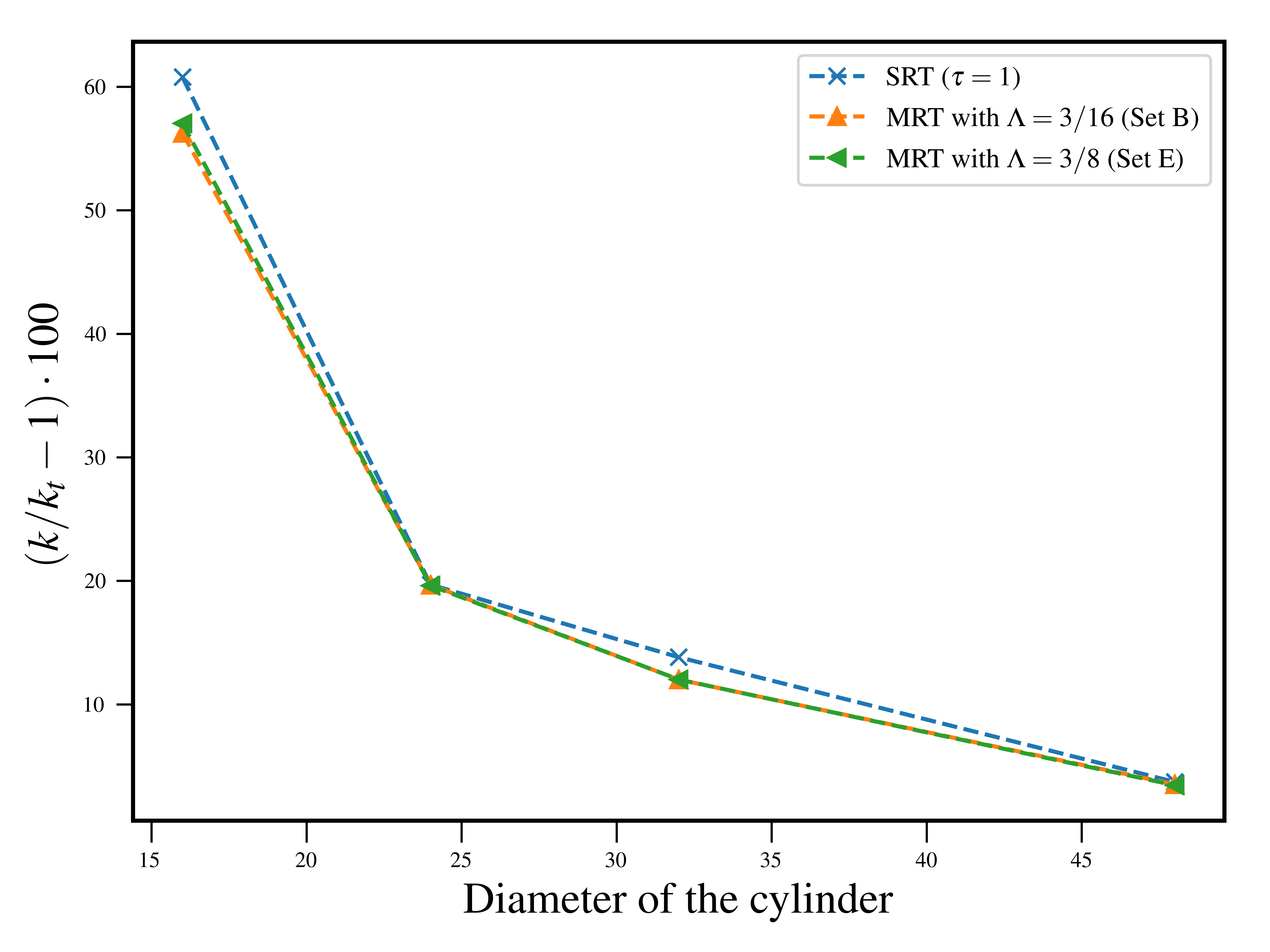
Figure 2: Errors in permeability of a circular channel as a function of the diameter of the channel for different relaxation parameters.

Next, we investigate the dependence of permeability predictions on the choices of relaxation parameters within the MRT collision model. For this purpose, we use three geometries with circular cross-sections: (i) a low-resolution channel where the diameter of the cylinder is 32 lattice units, (ii) a medium-resolution channel where the diameter is 64 lattice units, and (iii) a high-resolution channel where the diameter is 128 lattice units. The channel square cross section for the low, medium and high resolutions is $128\times 128,$ $256\times 256,$ and $512\times 512,$ respectively, such that the porosity of all of the geometries is maintained at $\phi=0.196.$ For each geometry, the viscosity is varied via the relation time, $\tau=\frac{1}{s_{\nu}}$ and the rest of the MRT relaxation parameters are varied as per Tab. 2. Figs. 3, 4, and 4 show the results of the simulations on the low, medium, and high-resolution geometries, respectively, where normalized permeability predictions are plotted against the relaxation time (viscosity).

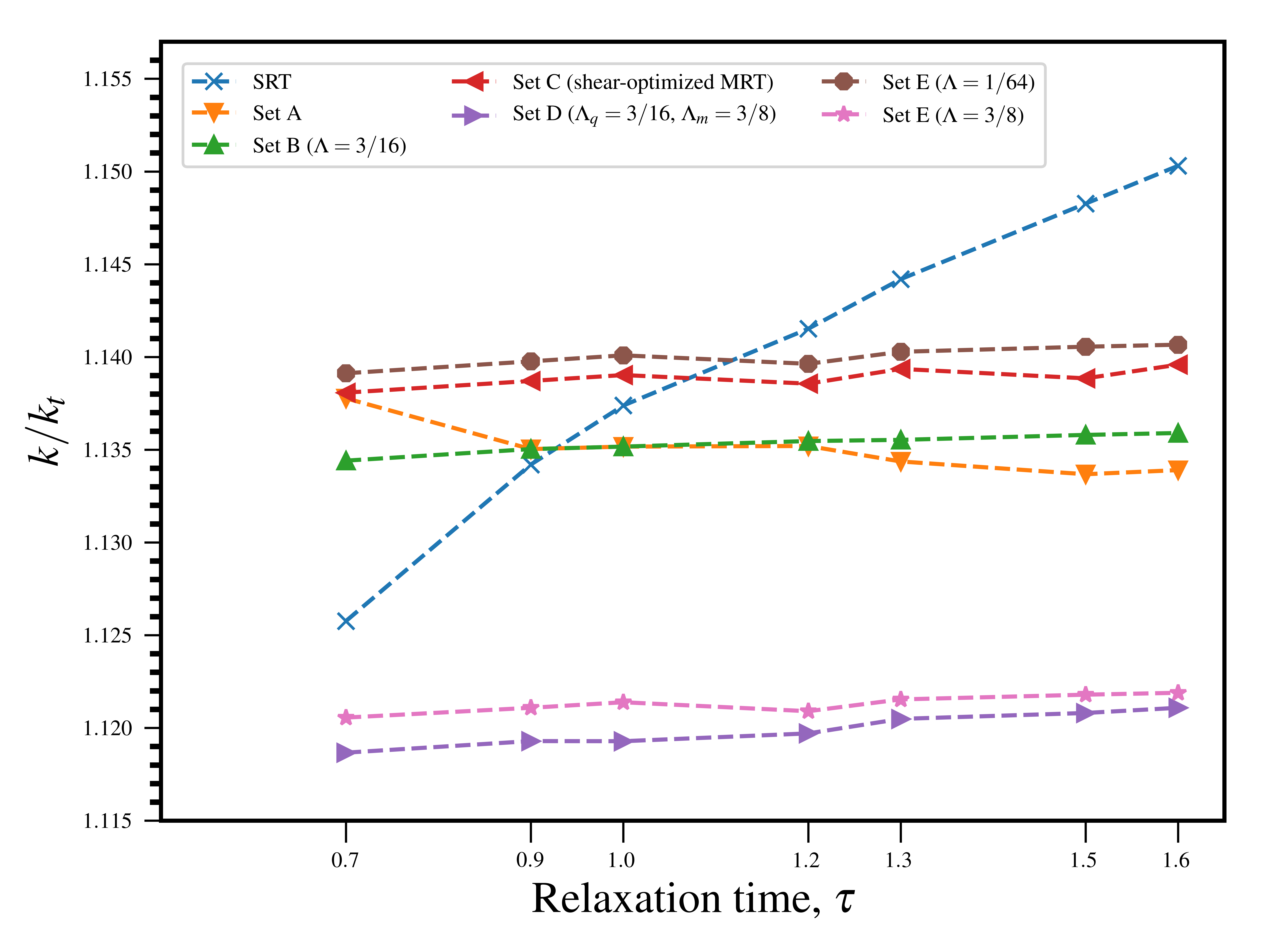
Figure 3: Normalized permeability $k/k_{ref}$ as a function of relaxation time for channel of size $128\times 128\times 128$ permeated by a circular pipe of diameter $D=32$ (low-resolution geometry).

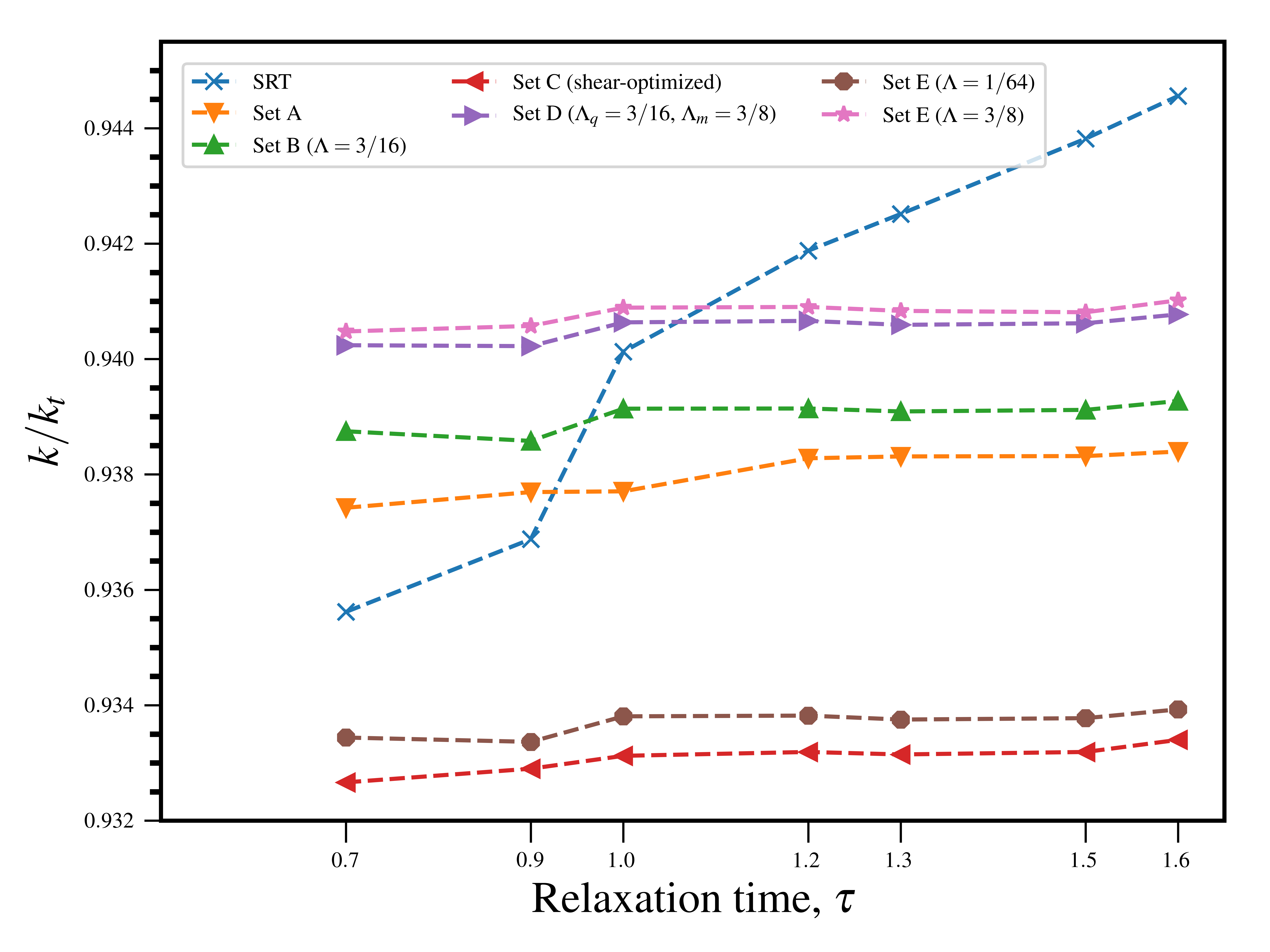
Figure 4: Normalized permeability$k/k_{ref}$ as a function of relaxation time for channel of size $256\times 256\times 256$ permeated by a circular pipe of diameter $D=64$ (medium-resolution geometry).

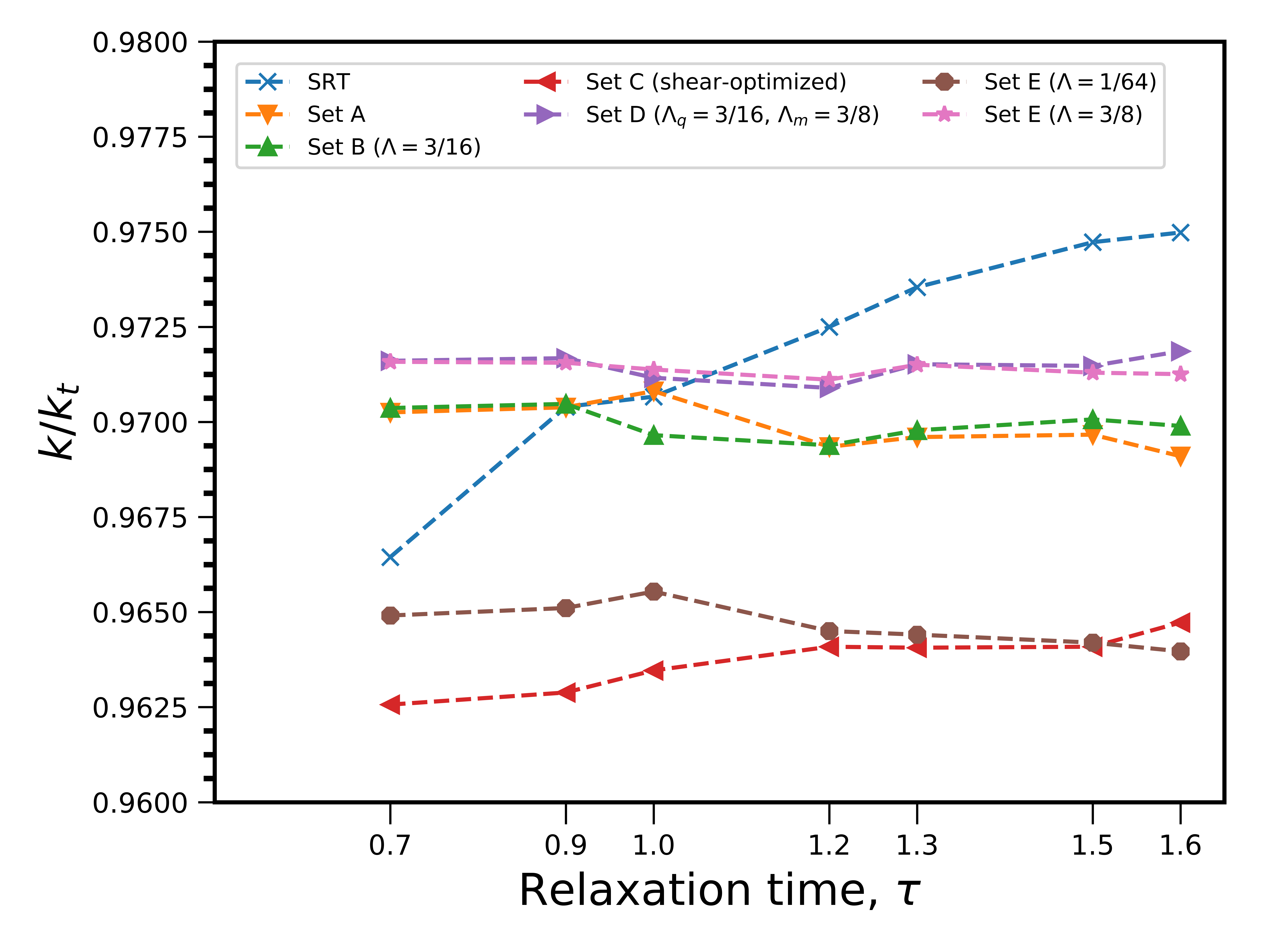
Figure 5: Errors in permeability as a function of relaxation time for channel of size $512\times 512\times 512$ permeated by a circular pipe of diameter $D=128$ (high-resolution geometry).

We first discuss the issue of viscosity independence. In the case of the channel of low-resolution, the errors are relatively high $(>12\%)$ for all sets of MRT parameters, as seen in Fig. 3. However, even such a coarse resolution, we can observe that variance of the normalized permeability over the range of $\tau$ $(\nu)$ as obtained with Sets B, D, and E are much smaller $(<0.2\%)$ compared to Set A and C, where the variance is about $0.5\%$ . This indicates that these parameters sets result in viscosity-independent permeability values. On the other hand, there is a much wider variance in errors for the SRT and Set A parameters. Similar trends can be seen in case of medium-resolution images. Notably, we can observe that the popular set of MRT parameters, i.e. Set C, has a slightly higher variance compared to Sets B, D, and E. For both the low and medium resolution cases, results obtained for SRT, and Sets A and B is consistent with the theoretical analysis which show that these cases do not follow rules of parameterization required to produce $\nu$-independent solutions of Stokes flow, see Rule (19) in [18]. For the high-resolution geometry, for all of the cases (except the SRT), the variance in computed permeability is much smaller compared to low and medium resolutions. For Sets B, D, and E, we observe error variance of less than 0.1% as compared to variance of about 0.3% for Sets A and C. We can also observe that the popular choice of parameters (Set C) shows slightly larger variation in permeability compared to Sets B, D and E, for both high and low resolution cases. Finally, across all resolutions, parameter sets B, D, and E consistently lead to $\nu-$independent results, and in general, dependence of permeability on $\nu$ reduces with increasing resolution of the pore-space.

Next, we consider the issue of accuracy. In low-resolution geometries we can observe that the errors are considerably higher irrespective of collision model and their parameters. Thus, as mentioned before, for under-resolved cases, all collision models (including MRT) can experience large errors irrespective of parameters. In parameter Sets B, D, and E, these errors remain fairly constant with variation of $\tau\,(\nu)$. For Set E, we observe that as $\Lambda$ increases from $1/64$ to $3/8,$ the accuracy increases for all three resolutions; thus $\Lambda=3/8$ leads to the smallest errors for each of three resolutions. Notably, in the case of low-resolution images, small values of $\Lambda$ result in much larger errors even compared to SRT. These trends indicate that, for a general porous medium, permeability obtained with the bounceback rule still depends on $\Lambda$ mainly due to unresolved pores. Moreover, spatial truncation error remain constant irrespective of $\tau$ and hence the permeability remains independent of $\tau\,(\nu)$.

Finally, we have observed that increasing $\tau$ leads to faster convergence for all cases, including for the SRT model. For instance, for the high resolution case with Set D parameters, the number of iterations required to converge decreased consistently from 19200 for $\tau=0.7$ to 7900 for $\tau=1.6.$ Similar trends were observed for all MRT sets of parameters (A-E) and all resolutions.

3.2 Channel with Triangular Cross-Section

The next model of porous media that we investigate is a channel with an opening of a triangular cross-section. Figure 1c show the details of this geometry. The reference permeability, $k_{ref}^{t},$ is computed as [27]:

$$k_{ref}^{t}=\frac{\sqrt{3}l^{4}}{320A}$$ (20)

where $l$ is the length of each side of the triangle and $A$ is cross-sectional area of the channel. The geometry creation and analysis procedure remains the same as described at the beginning of Sec. 3. In the results that follow, we considered a channel of size $256\times 256\times 256$ permeated with a triangle where each side measures 200 lattice units.

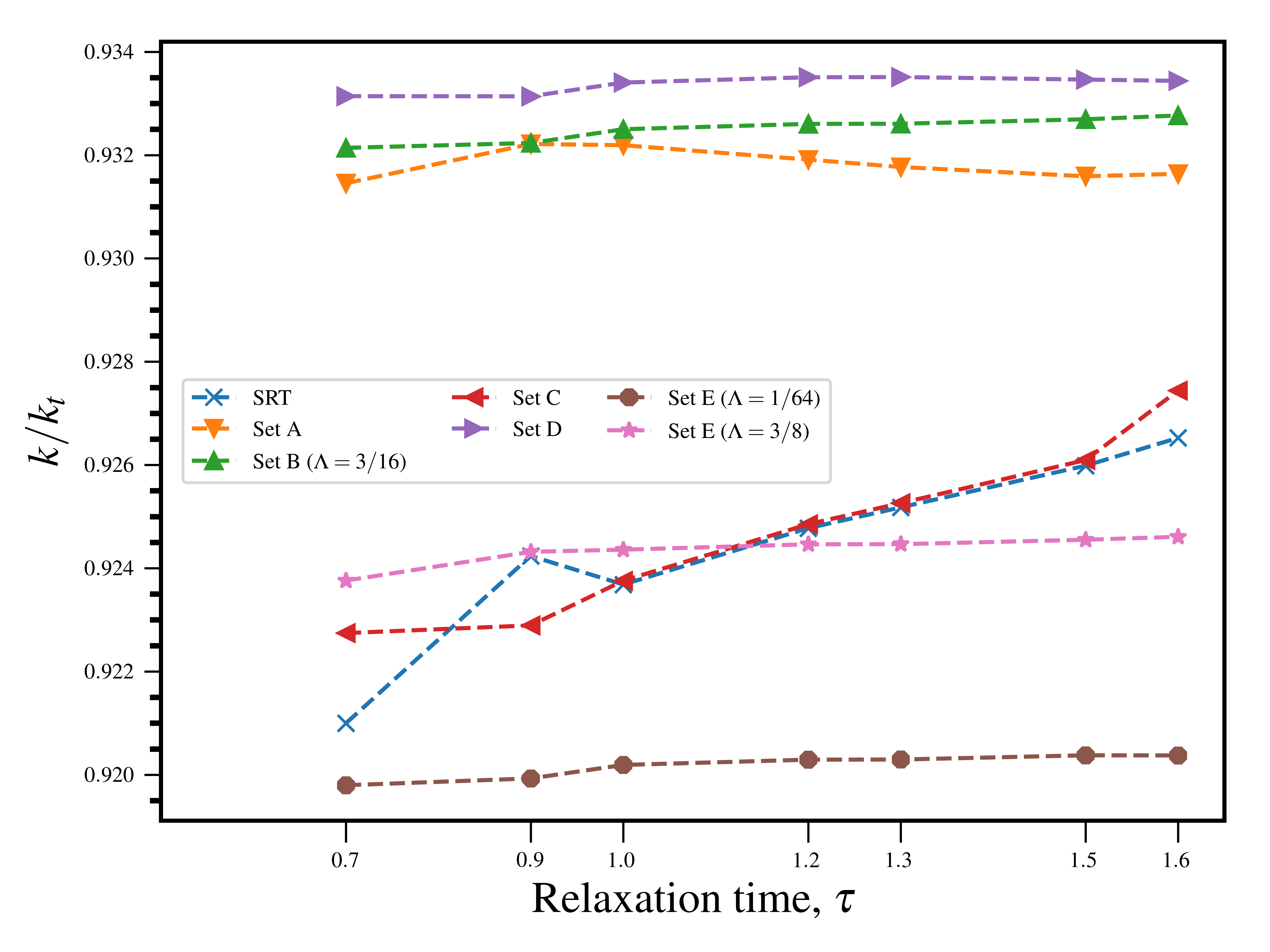
Figure 6: Normalized permeability function of relaxation time for channel of size $256\times 256\times 256$ permeated by a triangular cross-section of side length $l=200$ and $L=256$

In this case of a relatively high-resolution geometry, we can observe from Fig. 6, that parameter Sets D and E result in very low variance (less than 0.1 % in each case) in permeability prediction over the entire range of $\tau$ that were tested. Similar to the case of circular cross-section, we can observe that with Set C parameters, the variance is much stronger than in Sets D and E. Among the three sets of parameters, we find that Set D, where $\Lambda_{q}=3/16$ and $\Lambda_{m}=3/8,$ gives the most accurate overall predictions for the channel with triangular cross-section. We also observe that $k$ varies with $\Lambda,$ which indicates that overall accuracy of permeability predictions still depends on $\Lambda.$ This is, again, due to the finite-resolution of the images where solid boundary and pore-spaces may not be sufficiently resolved.

3.3 Sphere Pack

Random dense packing of identical (monodisperse) spheres serves as a useful geometry for the validation of pore-scale simulations for several reasons. First, experimental measurements can be easily obtained with sintered glass beads, and both empirical correlations and laboratory measurements are widely available. Second, random sphere packs are reasonable first-order approximations to sandstone, and yet are well defined mathematically. Third, a wide range of porosity and resolution can be obtained both in the laboratory and in simulations by uniform growth or shrinking of the spheres of the packing. In this study, we use the random sphere packing used in [31]; the entire image dataset is available online at [30]. The sphere pack dataset consists of 793 .bmp images, each of size 788x791. Fig. 7a shows a cross sectional view (in the direction of applied forcing) of the sphere pack and Fig. 7b shows a 3-D rendering of the geometry. The diameter of the spheres is 0.714 mm, and the voxel resolution is 7$\mu m$, giving a lattice nodes per sphere diameter,$\,d_{sp}\approx 100.$ The porosity of the sample is $\phi=0.34.$ We again point out that, in this work, we do not use curved boundary conditions to represent the surface of the spheres; instead, we use the bounceback boundary condition which the method of choice for pore-spaces obtained from microtomographic images.

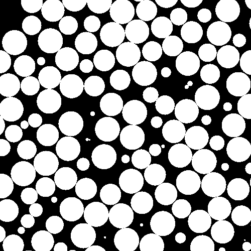
(a) Segmented image of a cross-section. Here BLACK indicate pore space and WHITE indicates solid or matrix space

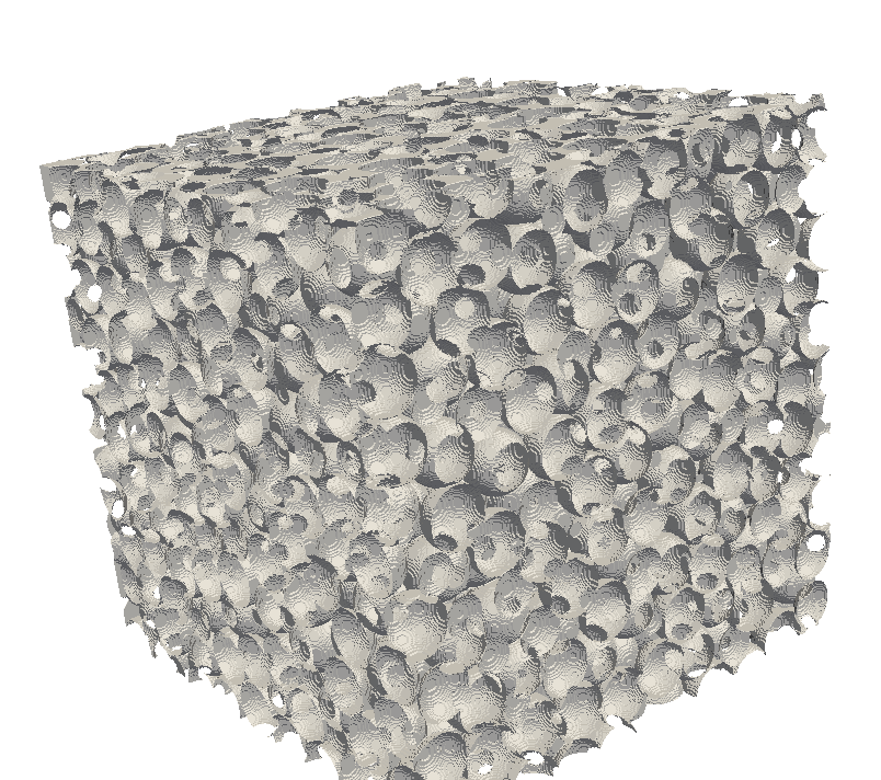
(b) 3-D rendering of the pore-space in random packing of spheres, where the gray voxel represent the pore/fluid space. Voxel resolution is $7\,\mu m$ and porosity of the packing is 0.34.

Figure 7: Random packing of mono-disperse spheres

As before, the images were converted to a .dat file which serves as an input for the LBM simulator. We apply the symmetry boundary condition on domain boundaries that are normal to the flow directions. Along the flow direction, a 5-layer padding is applied each at the inlet and outlet domain, as described in Sec. 2.3. The flow is imposed by applying a uniform body force in the positive $x$-direction: $F_{x}=\rho_{o}g_{x}$ with $\rho_{o}=1$ and $g_{x}=0.0001;$ no pressure gradient is explicitly imposed. From the steady-state solution (Stokes velocity field), the permeability is computed using Eqn. 17. For reference values, we use a value of $k_{ref}^{sp}=280,151mD$ which is the median value of permeability that was obtained using different LBM and non-LBM based fluid solvers on the same sphere pack image datasets as used in this study [31]. The reference sphere pack permeability translates to $k_{ref,lb}^{sp}=5.62$ l.u if expressed in LB units. Permeability in Darcy units can be converted to LB units, and vice-versa, via the relation $k_{D}$ =$k_{lb}\times\Delta x^{2}\times 0.9869,$ where $k_{D}$ is permeability in Darcy and $\Delta x$ is the voxel resolution in $m$.

The simulations are performed at three values of relaxation time, $\tau=\{0.7,1.0,1.5\}.$ Moreover, in addition to previously tested parameter sets, we also performed simulations with Set E parameters with two additional values of $\Lambda$, namely $\Lambda=1/64$ and $\Lambda=1,$ which represent a lower and higher bound on $\Lambda$ values as compared to the ’basic’ values of $\{\frac{1}{8},\frac{3}{16},\frac{1}{4},\frac{3}{8}\}.$

Fig. 8 shows the computed normalized permeability with various sets of parameters as a function of relaxation time (viscosity). As observed previously, the SRT permeability predictions increase with $\tau$ which is a a violation of Stokes flow. Predictions with Set A and shear-optimized parameter set (Set C) vary with viscosity but the variation is relatively small due to the (relatively) high-resolution nature of the voxels. Set B, D, and E, on the other hand, show very small variation in permeability with respect to viscosity which indicates that these parameter sets can generate viscosity-independent Stokes solutions and permeability for complex pore-spaces. We can also observe that Set A and Set B $(\Lambda=3/16)$ result in the most accurate predictions, followed by Set D $(\Lambda_{m}=3/16,\Lambda_{m}=3/8)$, and Set E with $\Lambda=3/8.$ We also observe that very small $(\Lambda=1/64)$ and very large ($\Lambda=1)$ values of $\Lambda$ lead to considerably inaccurate solutions, again, indicating that permeability predictions by MRT collision model (and the bounceback scheme) depend on $\Lambda$. This observation confirms the conclusions in Ref. [18] that $\Lambda\in[1/8,\,3/8]$ provides an optimal range for all resolutions and geometries. Finally, the above results, also indicate that for a given voxel resolution and pore-geometry, the optimal value of$\Lambda,$ in terms of accuracy, may have to be empirically determined within the bounds $\Lambda\in[1/8,\,3/8]$. Regarding convergence rates, similar to previous cases, we observed that increasing $\tau$ leads to faster convergence. For instance with the Set D parameters, the number of iterations required to converge decreased consistently from 6800 for $\tau=0.7$ to 3600 for $\tau=1.5.$ Similar trends were observed for the other sets (A-D) of parameters.

Note that at $\tau=1,$ the SRT predictions are very close to the reference solutions and solutions obtained from Sets B, D, and E. This indicates that the popular option of setting $\tau=1$ with SRT model might be produce reasonably accurate results if the voxel resolution of the micro-tomographic images is sufficiently high. The option of fixing $\tau=1$ for the SRT model, however, limits the option to expedite convergence, since increasing $\tau$ to improve convergence will quickly lead to erroneous predictions.

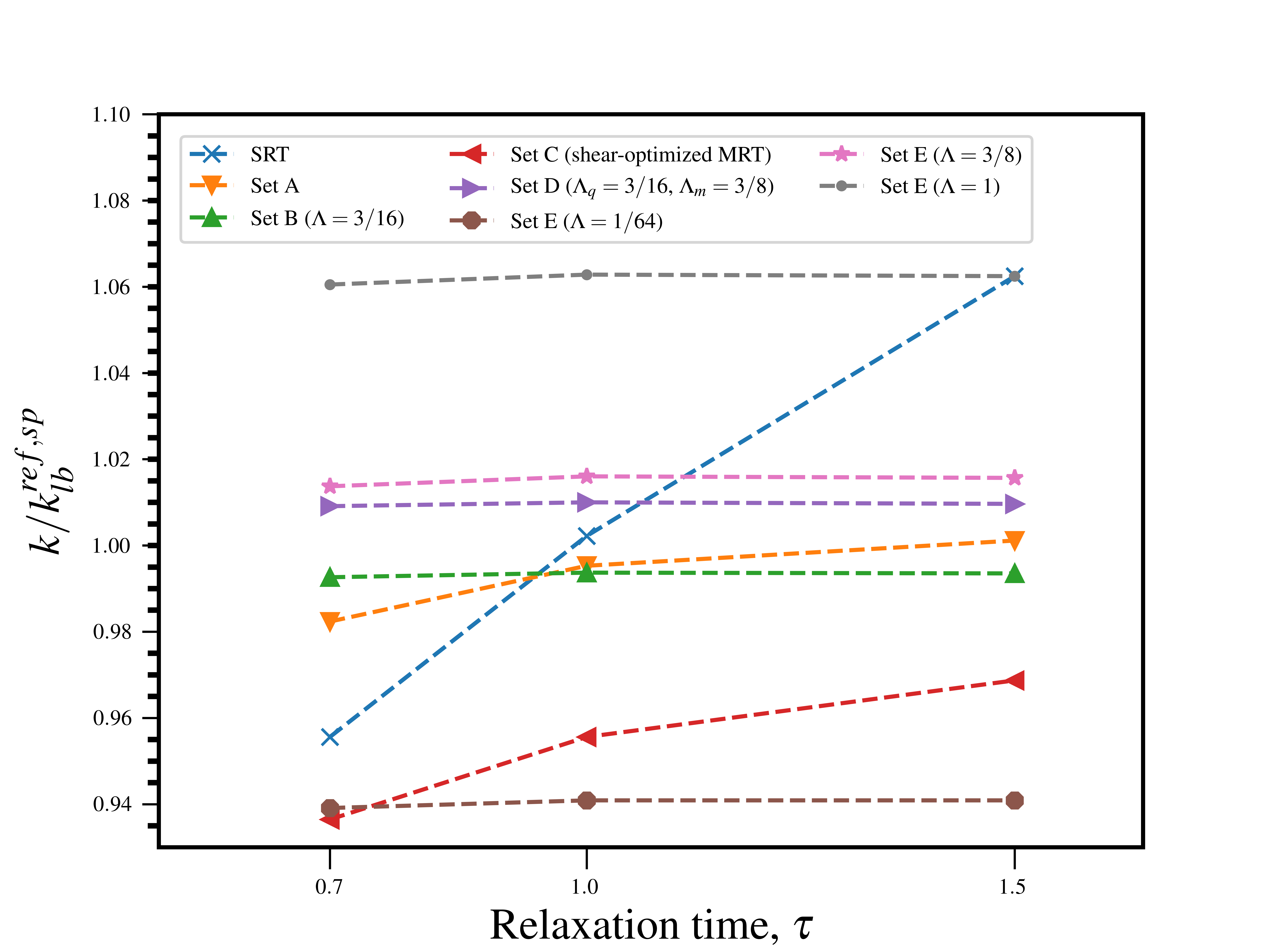
Figure 8: Normalized permeability of random packing of spheres obtained with different sets of relaxation parameters where $k_{ref},lb=5.6426\,l.u$ or $280,151\,mD.$

4 Conclusions

In this paper, we performed a systematic numerical evaluation of the different sets of relaxation parameters in the MRT model for modeling Stokes flow in 3-D microtomographic pore-spaces using the bounceback scheme. These sets of parameters are evaluated from the point of view of accuracy and an ability to generate viscosity-independent permeability solutions. Instead of tuning all six independent relaxation rates that are available in the D3Q19-MRT model, the sets that were analyzed have relaxation rates that depend on one or two independent parameters, namely $\tau$ and $\Lambda$. We tested elementary porous media at different image resolutions and a random packing of spheres at relatively high resolution. We can then conclude with the following remarks:

• For low-resolution micro-tomographic images, all collision models, including the MRT model and irrespective of the relaxation rates, produce solutions with very large numerical errors. Per Poiseuille law, since the overall flow rate is proportional to square of the cross-sectional area, the smallest pores have little impact of the overall flowrate. Therefore, as long as the larger pores are sufficiently resolved during imaging, the MRT model can produce reasonably accurate predictions. For low-permeability media, however, unresolved smallest pores are expected to be important.

• For a square channel permeated with a circular bore, among the various $\Lambda=\{\frac{1}{64},\frac{3}{16},\frac{3}{8}\}$, we observe that $\Lambda=3/8$ results in the most accurate solutions at all resolutions that were tested. Similarly, for a channel with triangular cross-section we find the following $\Lambda=3/16$ gives the most accurate results. On the other hand, for a dense random packing of identical spheres at 7$\mu m$ resolution, we observe that $\Lambda\in[1/8,\,3/8]$. This observation is consistent with the observations in [18]. If the very high resolution images are available, SRT with $\tau=1$ can also provide permeability with approximately the same accuracy as MRT models. However, since it leads viscosity-dependent permeability, the accuracy will vary depending choice of $\tau$.

• For the MRT model, sub-optimal choices of relaxation rates can lead to slower convergence and viscosity-dependent permeability predictions. In fact, it was observed that the popular choice of MRT parameters, as proposed in the seminal paper [5], result in permeability that depends (although weakly) on $\tau\,(\nu),$ a nonphysical artifact for simulating Stokes flow. Among the set of parameters that we tested, Sets B, D, and E consistently produce viscosity-independent (parameter-independent) results for all cases, for all resolutions, and over the entire range of $\tau$. We also observed that a larger $\tau$ leads to a substantial reduction in the number of iterations required for convergence without any adverse effects on accuracy. Therefore, if a MRT implementation/code is to be used for pore-scale Stokes flow, then it is recommended that the relaxation rates $(s_{0}-s_{18})$ should be chosen as per Sets B, D, or E (listed in Table 2) and $\tau$ be chosen in the range $\tau\in[1.2,1.5]$, in order to obtain viscosity-independent results, including permeability. For Set E specifically, choosing $\Lambda\in[1/8,\,3/8]$ and $\tau\in[1.0,1.3]$ can result in overall superior accuracy, convergence rate, and parameter-independent predictions.

Acknowledgments

Financial support from the Energy and Environment Institute (EEi) at Rice University is gratefully acknowledged. This work was supported in part by the Data Analysis and Visualization Cyberinfrastructure funded by the National Science Foundation (NSF) under grant OCI-0959097 and Rice University. We also thank the developers of Palabos for their technical assistance.

References

- [1] Benjamin Ahrenholz, Jonas Tolke, and Manfred Krafczyk. Lattice-boltzmann simulations in reconstructed parametrized porous media. International Journal of Computational Fluid Dynamics, 20(6):369–377, 2006.
- [2] Carl Fredrik Berg, Olivier Lopez, and Håvard Berland. Industrial applications of digital rock technology. Journal of Petroleum Science and Engineering, 157:131–147, 2017.
- [3] Mohamed Bouzidi, Mouaouia Firdaouss, and Pierre Lallemand. Momentum transfer of a boltzmann-lattice fluid with boundaries. Physics of fluids, 13(11):3452–3459, 2001.
- [4] Tom Bultreys, Wesley De Boever, and Veerle Cnudde. Imaging and image-based fluid transport modeling at the pore scale in geological materials: A practical introduction to the current state-of-the-art. Earth-Science Reviews, 155:93–128, 2016.
- [5] Dominique dHumières. Multiple–relaxation–time lattice boltzmann models in three dimensions. Philosophical Transactions of the Royal Society of London A: Mathematical, Physical and Engineering Sciences, 360(1792):437–451, 2002.
- [6] Dominique dHumieres and Irina Ginzburg. Viscosity independent numerical errors for lattice boltzmann models: from recurrence equations to magic collision numbers. Computers & Mathematics with Applications, 58(5):823–840, 2009.
- [7] Amir Eshghinejadfard, László Daróczy, Gábor Janiga, and Dominique Thévenin. Calculation of the permeability in porous media using the lattice boltzmann method. International Journal of Heat and Fluid Flow, 62:93–103, 2016.
- [8] Ehsan Fattahi, Christian Waluga, Barbara Wohlmuth, Ulrich Rüde, Michael Manhart, and Rainer Helmig. Lattice boltzmann methods in porous media simulations: From laminar to turbulent flow. Computers & Fluids, 140:247–259, 2016.
- [9] Bruno Ferréol and Daniel H. Rothman. Lattice-boltzmann simulations of flow through fontainebleau sandstone. Transport in Porous Media, 20(1):3–20, Aug 1995.
- [10] John Finney. Finney packing of spheres. http://www.digitalrocksportal.org/projects/47, 2016.
- [11] JT Fredrich, AA DiGiovanni, and DR Noble. Predicting macroscopic transport properties using microscopic image data. Journal of Geophysical Research: Solid Earth, 111(B3), 2006.
- [12] I Ginzbourg and PM Adler. Boundary flow condition analysis for the three-dimensional lattice boltzmann model. Journal de Physique II, 4(2):191–214, 1994.
- [13] Irina Ginzburg. Variably saturated flow described with the anisotropic lattice boltzmann methods. Computers & fluids, 35(8-9):831–848, 2006.
- [14] Irina Ginzburg and Dominique dHumieres. Multireflection boundary conditions for lattice boltzmann models. Physical Review E, 68(6):066614, 2003.
- [15] Irina Ginzburg, Frederik Verhaeghe, and Dominique dHumieres. Two-relaxation-time lattice boltzmann scheme: About parametrization, velocity, pressure and mixed boundary conditions. Communications in computational physics, 3(2):427–478, 2008.
- [16] Zhaoli Guo, Baochang Shi, TS Zhao, and Chuguang Zheng. Discrete effects on boundary conditions for the lattice boltzmann equation in simulating microscale gas flows. Physical Review E, 76(5):056704, 2007.
- [17] Zhaoli Guo and Chang Shu. Lattice Boltzmann method and its applications in engineering, volume 3. World Scientific, 2013.
- [18] Siarhei Khirevich, Irina Ginzburg, and Ulrich Tallarek. Coarse-and fine-grid numerical behavior of mrt/trt lattice-boltzmann schemes in regular and random sphere packings. Journal of Computational Physics, 281:708–742, 2015.
- [19] Timm Krüger, Halim Kusumaatmaja, Alexandr Kuzmin, Orest Shardt, Goncalo Silva, and Erlend Magnus Viggen. The lattice boltzmann method, 2017.
- [20] Pierre Lallemand and Li-Shi Luo. Theory of the lattice boltzmann method: Dispersion, dissipation, isotropy, galilean invariance, and stability. Physical Review E, 61(6):6546, 2000.
- [21] Li-Shi Luo, Manfred Krafczyk, and Wei Shyy. Lattice boltzmann method for computational fluid dynamics. Encyclopedia of Aerospace Engineering, pages 651–660, 2010.
- [22] Li-Shi Luo, Wei Liao, Xingwang Chen, Yan Peng, Wei Zhang, et al. Numerics of the lattice boltzmann method: Effects of collision models on the lattice boltzmann simulations. Physical Review E, 83(5):056710, 2011.
- [23] RS Maier and RS Bernard. Lattice-boltzmann accuracy in pore-scale flow simulation. Journal of Computational Physics, 229(2):233–255, 2010.
- [24] C Manwart, U Aaltosalmi, A Koponen, R Hilfer, and J Timonen. Lattice-boltzmann and finite-difference simulations for the permeability for three-dimensional porous media. Physical Review E, 66(1):016702, 2002.
- [25] Nicos S Martys and Hudong Chen. Simulation of multicomponent fluids in complex three-dimensional geometries by the lattice boltzmann method. Physical Review E, 53(1):743, 1996.
- [26] Keijo Mattila, Tuomas Puurtinen, Jari Hyväluoma, Rodrigo Surmas, Markko Myllys, Tuomas Turpeinen, Fredrik Robertsen, Jan Westerholm, and Jussi Timonen. A prospect for computing in porous materials research: Very large fluid flow simulations. Journal of Computational Science, 12:62–76, 2016.
- [27] Gary Mavko, Tapan Mukerji, and Jack Dvorkin. The rock physics handbook: Tools for seismic analysis of porous media. Cambridge university press, 2009.
- [28] Ariel Narváez, Thomas Zauner, Frank Raischel, Rudolf Hilfer, and Jens Harting. Quantitative analysis of numerical estimates for the permeability of porous media from lattice-boltzmann simulations. Journal of Statistical Mechanics: Theory and Experiment, 2010(11):P11026, 2010.
- [29] Chongxun Pan, Li-Shi Luo, and Cass T Miller. An evaluation of lattice boltzmann schemes for porous medium flow simulation. Computers & fluids, 35(8-9):898–909, 2006.
- [30] Nishank Saxena. Data for: References and benchmarks for pore-scale flow simulated using micro-ct images of porous media and digital rocks, 2017.
- [31] Nishank Saxena, Ronny Hofmann, Faruk O Alpak, Steffen Berg, Jesse Dietderich, Umang Agarwal, Kunj Tandon, Sander Hunter, Justin Freeman, and Ove Bjorn Wilson. References and benchmarks for pore-scale flow simulated using micro-ct images of porous media and digital rocks. Advances in Water Resources, 109:211–235, 2017.
- [32] L Talon, D Bauer, N Gland, S Youssef, H Auradou, and I Ginzburg. Assessment of the two relaxation time lattice-boltzmann scheme to simulate stokes flow in porous media. Water Resources Research, 48(4), 2012.
- [33] Palabos Team. Palabos:open-source lbm software. http://www.palabos.org/, 2009–2017.
- [34] Dorthe Wildenschild and Adrian P Sheppard. X-ray imaging and analysis techniques for quantifying pore-scale structure and processes in subsurface porous medium systems. Advances in Water Resources, 51:217–246, 2013.
- [35] Lina Xu, Parthib Rao, and Laura Schaefer. A novel scheme for curved moving boundaries in the lattice boltzmann method. International Journal of Modern Physics C, 27(12):1650144, 2016.
- [36] PG Young, TBH Beresford-West, SRL Coward, B Notarberardino, B Walker, and A Abdul-Aziz. An efficient approach to converting three-dimensional image data into highly accurate computational models. Philosophical Transactions of the Royal Society of London A: Mathematical, Physical and Engineering Sciences, 366(1878):3155–3173, 2008.
- [37] Yan Zaretskiy, Sebastian Geiger, Ken Sorbie, and Malte Forster. Efficient flow and transport simulations in reconstructed 3d pore geometries. Advances in Water Resources, 33(12):1508 – 1516, 2010.