Practical sampling schemes for quantum phase estimation

Abstract

In this work we consider practical implementations of Kitaev’s algorithm for quantum phase estimation. We analyze the use of phase shifts that simplify the estimation of successive bits in the estimation of unknown phase $\varphi$. By using increasingly accurate shifts we reduce the number of measurements to the point where only a single measurements in needed for each additional bit. This results in an algorithm that can estimate $\varphi$ to an accuracy of $2^{-(m+2)}$ with probability at least $1-\epsilon$ using $N_{\epsilon}+m$ measurements, where $N_{\epsilon}$ is a constant that depends only on $\epsilon$ and the particular sampling algorithm. We present different sampling algorithms and study the exact number of measurements needed through careful numerical evaluation, and provide theoretical bounds and numerical values for $N_{\epsilon}$.

1 Introduction

Given a unitary operator $U$ and one of its eigenvectors $|{\xi}\rangle$, we would like to obtain an accurate estimate of the corresponding eigenvalue $\lambda$, which, as a result of unitarity, can be written as $\lambda=e^{i2\pi\varphi}$ with $\varphi\in[0,1)$. The quantum phase estimation problem considers finding an estimate of the phase $\varphi$, from which the estimate of $\lambda$ is then easily found. The importance of quantum phase estimation is highlighted by the wide range of applications that rely on it, including Shor’s prime factorization algorithm [13], quantum chemistry [3, 16, 12], and quantum Metropolis sampling [15].

Figure 1: Quantum circuit for phase estimation of $U^{s}$.

The two main approaches to quantum phase estimation are the Fourier-based approach described in [5, 8, 11], and Kitaev’s algorithm [8, 9], which we study in this work. The quantum circuit central to Kitaev’s algorithm is illustrated in Figure 1. Assuming an initial state of $|{0}\rangle|{\xi}\rangle$, the circuit first applies a Hadamard operation on the first qubit, followed by a phase-shift operation

$$Z_{\theta}=\left[\begin{matrix}1&0\\ 0&e^{i2\pi\theta}\end{matrix}\right].$$

The circuit then applies $U^{s}$ on the $|{\xi}\rangle$ qubits, conditioned on the first qubit, where

$$U^{s}|{\xi}\rangle=\lambda^{s}|{\xi}\rangle=e^{i2\pi(s\varphi)}|{\xi}\rangle.$$ (1)

Finally, a second Hadamard operation is applied on the first qubit followed by a not gate and measurement. The circuit performs the following mapping:

$$|{0}\rangle\otimes|{\xi}\rangle\rightarrow\left(\frac{1-e^{i2\pi(s\varphi+\theta)}}{2}|{0}\rangle+\frac{1+e^{i2\pi(s\varphi+\theta)}}{2}|{1}\rangle\right)\otimes|{\xi}\rangle$$

Measuring the first qubit therefore returns 1 with probability

$$P_{\theta}(1\mid\varphi)=\left|\frac{1+e^{i2\pi(\varphi+\theta)}}{2}\right|^{2}=\frac{1+\cos(2\pi(\varphi+\theta))}{2},$$

and 0 otherwise. By appropriately choosing $\theta$ we can obtain information on the sine and cosine of $\varphi$, since

$$\cos(2\pi\varphi)=2P_{0}(1\mid\varphi)-1,\quad\mbox{and}\quad\sin(2\pi\varphi)=2P_{-1/4}(1\mid\varphi)-1.$$ (2)

Repeated measurements of the quantum circuit with $\theta=0$ and $\theta=-1/4$ allow us to approximate $P_{0}$ and $P_{-1/4}$, from which the sine and cosine values and subsequently $\tilde{\varphi}$ can then be determined.

Throughout this work we use the convention that angles $\varphi$, $\theta$, and $\omega$ are expressed in radians divided by $2\pi$, whereas angles $\alpha$ are always expressed in radians. We frequently use

$$p_{x}(\alpha)=\frac{1+\cos(\alpha)}{2},\quad\mathrm{and}\quad p_{y}(\alpha)=\frac{1+\sin(\alpha)}{2},$$

and write $p_{x}$ and $p_{y}$ when the dependency on $\alpha$ is clear.

2 Kitaev’s algorithm

The goal in Kitaev’s algorithm [9] is to obtain the approximation

$$\tilde{\varphi}=.\overline{\beta^{\prime}_{1}\beta^{\prime}_{2}\cdots\beta^{\prime}_{m}\beta^{\prime}_{m+1}\beta^{\prime}_{m+2}}=\sum_{j=1}^{m+2}2^{-j}\beta^{\prime}_{j},$$

for $\varphi=.\overline{\beta_{1}\beta_{2}\beta_{3}\cdots}$, such that $|\varphi-\tilde{\varphi}|\leq 2^{-(m+2)}$ holds with probability at least $1-\epsilon$. The key principle behind the algorithm lies in the fact that using $U^{s}$ in (1) with $s=2^{j-1}$ gives measurements about $s\varphi$, and therefore amounts to shifting the bits in $\varphi$ to the left by $j-1$ positions:

$$\varphi_{j}:=2^{j-1}\varphi\equiv.\overline{\beta_{j}\beta_{j+1}\beta_{j+2}\cdots}\ \mathrm{mod}\ 1.$$

The multiplicative factor of $2\pi$ causes the phase to be invariant to the integer part $\overline{\beta_{1}\cdots\beta_{j-1}}$, which can therefore be omitted. As a result, by choosing $j$ we can work with the bitstring starting from any $\beta_{j}$. Using this, the first step of Kitaev’s algorithm is to choose $j=m$ and estimate $\tilde{\varphi}_{j}=.\overline{\beta^{\prime}_{m}\beta^{\prime}_{m+1}\beta^{\prime}_{m+2}}$ such that $|\varphi_{j}-\tilde{\varphi}_{j}|\leq 1/8$ with probability at least $1-\bar{\epsilon}_{m}$. This is done by taking sufficiently many samples (discussed in detail in Section 4) to estimate $\cos(2\pi\varphi_{j})$ and $\sin(2\pi\varphi_{j})$ such that the approximated angle $\omega_{j}$ deviates from $\varphi_{j}$ by at most $1/16$ with probability at least $1-\bar{\epsilon}_{m}$. The angle $\omega_{j}$ is then quantized (rounded) to the nearest integer multiple of $1/8$ modulo 1 to obtain $\tilde{\varphi}_{j}$. With a maximum quantization error of $1/16$, this amounts to an accuracy of at least $1/8$.

The second stage of the algorithm iteratively adds one new bit $\beta^{\prime}_{j}$ per step, for $j=m-1,\ldots,1$. For each step we first obtain a $1/16$ accurate approximation $\omega_{j}$ of $\varphi_{j}$ with probability at least $1-\bar{\epsilon}_{j}$ using the technique outlined above. Next, we enforce consistency using the bitstring known so far and set

$$\beta^{\prime}_{j}:=\begin{cases}0&\mathrm{if}\ |.\overline{0\beta^{\prime}_{j+1}\beta^{\prime}_{j+2}}-\mbox{$\omega_{j}$}|<1/4,\\ 1&\mathrm{if}\ |.\overline{1\beta^{\prime}_{j+1}\beta^{\prime}_{j+2}}-\mbox{$\omega_{j}$}|<1/4.\end{cases}$$

Using a union bound on the error probabilities, it can be seen that the algorithm succeeds with probability at least $1-\sum_{j=1}^{m}\bar{\epsilon}_{j}$. Choosing $\epsilon_{j}=\epsilon/m$ we can therefore ensure with probability at least $1-\epsilon$ that all approximate angles $\omega_{j}$ are valid, in which case $\tilde{\varphi}$ will be $2^{-(m+2)}$ accurate. A graphical illustration of Kitaev’s algorithm is given in Figure 2.

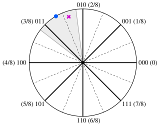
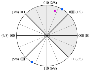
(a)	(b)

Figure 2: (a) Estimation of the angle $\phi_{j}$ indicated by the blue dot is done by obtaining estimates of the sine and cosine values (indicated by the purple cross), from which an approximate angle $\omega_{j}$ and quantization ($\underline{01}$0) can be obtained. Angle $\phi_{j}$ is equal to $2\phi_{j-1}$ modulo 1, and could therefore originate from either of the blue dots in plot (b). Fixing the last two bits to the leading two from the previous estimates gives points closest to $0\underline{01}$, indicated by the shaded region, or closest to $1\underline{01}$. Measuring the purple cross determines $\beta^{\prime}_{j}=0$.

The estimation of the sine or cosine terms in (2) with accuracy $\delta$ requires estimation of the probability terms to accuracy $\delta/2$. Let $s_{1},\ldots,s_{n}$, be i.i.d. samples of a Bernoulli distribution with probability of success $p=1-P_{\theta}(1)$. Denoting $\tilde{p}_{n}=(1/n)\sum_{i=1}^{n}s_{i}$, then it follows from the Chernoff bound that

$$\mathrm{Pr}[|p-\tilde{p}_{n}|\geq\delta/2]\leq 2e^{-\delta^{2}n/2}.$$ (3)

We require that the probability $2e^{-\delta^{2}n/2}$ be bounded by $\bar{\epsilon}$, which is guaranteed for

$$n\geq n(\delta,\epsilon)=\frac{2}{\delta^{2}}\log(2/\bar{\epsilon}).$$ (4)

For the theoretical complexity of Kitaev’s algorithm, note that $m$ angle estimations $\omega_{j}$ are used, each requiring approximate sine and cosine values, therefore yielding a total of $2m$ estimations. By choosing $\bar{\epsilon}=\epsilon/2m$ we obtain an overall sample complexity of $\frac{4m}{\delta^{2}}\log(4m/\epsilon)=\mathcal{O}(m\log(m/\epsilon))$.

3 Improvements using phase shifts

As a practical improvement to steps in the second stage of Kitaev’s algorithm, consider the situation shown in Figure 2(b). The exact value of $\varphi_{j}$ is equal to either $(0+\varphi_{j+1})/2$, or $(1+\varphi_{j+1})/2$, as indicated by the blue dots. Using the first two bits of the binary representation for $\tilde{\varphi}_{j+1}$, in this case 01, we therefore know that $\varphi_{j}$ is at most 1/8 away from either 001 or 101. Using this information, we can first rotate $\varphi_{j}$ by the reference angle, in this case 001, to obtain a new angle that is 1/8 away from either 000 or 100, as illustrated in Figure 3(a). Now, instead of approximating both sine and cosine we only need to determine the sign of the cosine, which requires far fewer measurements. We then set $\beta^{\prime}_{j}$ based on the sign: if it is positive we set $\beta^{\prime}_{j}=0$, otherwise we set $\beta^{\prime}_{j}=1$. We can further improve this scheme by maintaining all known bits and rotate by 0010, instead of by the truncated version 001. Doing so we obtain an angle that is now at most 1/16 away from 0 or 1/2, as shown in Figure 3(b). By using the full binary string $\tilde{\varphi}_{j+1}/2$ at each stage, we get increasingly small deviations from 0 or 1/2, which increases the magnitude of the cosine value and reduces the number of measurements needed to accurately determine the correct sign.

Increasingly accurate rotations

The use of existing measurements to correct or zero out portions of the binary representation in iterative phase estimation was described earlier by [4, 10] along with its connection to phase estimation based on the quantum Fourier transformation. Here we analyze the measurement complexity in detail (see also [6] for a high-level analysis). Given that the bits $\beta^{\prime}_{j}$ are determined in reverse order (that is, from least to most significant), we switch to working with iterations, such that iteration $k\in[1,m]$ determines $\beta^{\prime}_{m+1-k}$. We now consider iterations $k\geq 2$, which comprise the second stage of the algorithm. At each iteration in the second stage we need to determine the sign of the cosine of the shifted angle. In terms of measurements, this amounts to sampling a majority of either zeros or ones. For the number of measurements we have the following result.

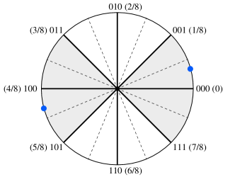
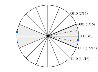
(a)	(b)

Figure 3: Application of a phase shift ensures that the unknown angle (indicated by the blue dot) lies within one of the highlighted wedges centered on the horizontal axis. The more accurate the reference angle, the smaller the wedge, as shown in (a) with maximum deviation $1/8$, and (b) $1/16$.

Theorem 3.1.

Let $\alpha\in(0,\pi/2)$. Then we can correctly distinguish angles from the sets $[-\alpha,\alpha]$ and $[\pi-\alpha,\pi+\alpha]$ with probability at least $1-\epsilon$ by checking whether the majority of $n$ measurements is 1 or 0, whenever

$$n\geq\frac{\log(1/\epsilon)}{\log(1/\sin(\alpha))}.$$ (5)

Proof.

Assume that unknown angle lies in the range $[-\alpha,\alpha]$ and denote by $p=(1+\cos(\alpha))/2$. The probability that at most $k$ out of $n$ measurements are 1, with $k<np$ is bounded by [2]:

$$\mathrm{Pr}(X\leq k)\leq\exp\left(-nD(k/n\|p)\right),$$ (6)

where $D(a\|p)$ denotes the relative entropy

$$D(a\|p)=a\log\left(\frac{a}{p}\right)+(1-a)\log\left(\frac{1-a}{1-p}\right).$$

We want the majority of the measurements to be 1 and an error therefore occurs whenever $k\leq n/2$. Choosing $k=n/2$, which is allowed since $p>1/2$, gives $a=1/2$ and an error $\epsilon^{\prime}$ bounded by

$$\epsilon^{\prime}\leq\exp\left(-\frac{n}{2}\log(1/(4p(1-p)))\right)$$ (7)

To simplify, note that

$$4p(1-p)=4\left(\frac{1+\cos(\alpha)}{2}\right)\left(\frac{1-\cos(\alpha)}{2}\right)=1-\cos^{2}(\alpha)=\sin^{2}(\alpha).$$ (8)

We want to ensure that the right-hand side of (7) is less than or equal to $\epsilon$. Taking logarithms and simplification then gives the desired result. The result for $[\pi-\alpha,\pi+\alpha]$ follows similarly. ∎

At iteration $k$ we apply a phase shift based on the angle from the previous iteration, and Theorem 3.1 therefore applies with $\alpha$ equal to $\alpha_{k}=\pi/2^{k+1}$ (as an example, at iteration $k=2$ we have a maximum deviation of 1/16 or $\pi/8$). When taking a single measurement, the probability of failure is $1-p_{k}$ where $p_{k}=p_{x}(\alpha_{k})$. In the special case where $k$ is such that $1-p_{k}\leq\bar{\epsilon}$, it is therefore follows that only a single sample is needed. It holds that

$$1-p_{k} = (1-\cos(\pi/2^{k+1}))/2$$ (9)

$$= \sin^{2}(\pi/2^{k+2})$$

$$\leq \pi^{2}/2^{2(k+2)},$$

where we use the identity $1-\cos(x)=2\sin^{2}(x/2)$ in the second line and $\sin(x)\leq x$ for $x\geq 0$ in the last. We want to find the value of $k$ such that iterations $k$ through $m$ each require only a single measurement and have a combined error bounded by $\bar{\epsilon}$. Choosing $\bar{\epsilon}=\epsilon/k$, gives the requirement

$$\sum_{j=k}^{m}(1-p_{j})\leq\epsilon/k$$

Bounding the left-hand side as

$$\sum_{j=k}^{m}(1-p_{j})\leq\sum_{j=k}^{m}\pi^{2}/2^{2(j+2)}\leq\pi^{2}\sum_{j=k}^{\infty}(1/4)^{j+2}=\frac{4\pi^{2}}{3}\left(\frac{1}{4}\right)^{k+2}=\frac{\pi^{2}}{12}4^{-k},$$ (10)

we obtain the sufficient condition

$$4^{-k}\leq\frac{12\epsilon}{k\pi^{2}}.$$ (11)

Taking base-two logarithm and rearranging gives

$$2k-\log_{2}(k/12)\geq\log_{2}(\pi^{2}/\epsilon).$$

It can be verified that $\log_{2}(k/12)<k/22$ for $k\geq 0$, and we can therefore choose

$$k\geq k_{\epsilon}:=\left\lceil\frac{22}{43}\log_{2}(\pi^{2}/\epsilon)\right\rceil\!.$$ (12)

The value of $k_{\epsilon}$ does not depend on $m$ and satisfies that for $k_{\epsilon}\geq 2$ for all $\epsilon\in(0,1]$. The bound on the sum of errors for iterations $k\geq k_{\epsilon}$ in (10) can be seen to apply for any $m$. Denote by $N_{\epsilon}$ the total number of measurements taken in the first $k_{\epsilon}-1$ iterations, each with an error not exceeding $\bar{\epsilon}$. When $m<k_{\epsilon}$ it is clear that at most $N_{\epsilon}$ samples are needed. When $m\geq k_{\epsilon}$ we need to take an additional sample for each of the remaining $m-k_{\epsilon}+1$ steps. The overall sampling complexity is therefore bounded by $N_{\epsilon}+m$, where $N_{\epsilon}$ depends only on $\epsilon$ and the sampling methods used for the first $k_{\epsilon}-1$ iterations. The work by Svore et al. [14] proposes a phase estimation algorithm with complexity $\mathcal{O}(m\log^{*}(m))$. Unlike the proposed method, however, their algorihm allows parallelization and the use of clusters, and does not require arbitrarily accurate phase shifts, which can be expensive from a circuit perspective (see the Discussion section for more details).

4 Practical sampling schemes

In this section we consider different sampling schemes and study the number of samples needed to attain a desired accuracy with a given error rate. For the evaluation of the error rate, we consider the measurements as a Binomial random variable by counting the number of successful measurements (which could be either 0 or 1, depending on the context). In order to determine the angle to a certain accuracy using $n$ measurements, the number of successful measurements $X$ typically needs to fall in some set $\mathcal{K}\subseteq[n]$, where $[n]$ denotes the set $\{0,1,\ldots.n\}$. For $p=p_{x}(\alpha)$ this is satisfied with probability

$$\mathrm{Pr}(\mathcal{K}\mid n,\alpha)=\sum_{k\in\mathcal{K}}{n\choose k}p^{k}(1-p)^{n-k}.$$ (13)

We also require two-dimensional settings with probabilities $p_{x}$ and $p_{y}$ and $\mathcal{K}\in[n]\times[n]$, given by

$$\mathrm{Pr}(\mathcal{K}\mid n,\alpha)=\sum_{(k_{x},k_{y})\in\mathcal{K}}{n\choose k_{x}}{n\choose k_{y}}p_{x}^{k_{x}}(1-p_{x})^{n-k_{x}}p_{y}^{k_{y}}(1-p_{y})^{n-k_{y}}.$$ (14)

The error rate is then given by $1-\mathrm{Pr}(\mathcal{K})$, and the goal is to find the minimum $n$ for which the error is below some threshold $\bar{\epsilon}$. In addition to providing bounds, we use the GNU multi-precision arithmetic library to evaluate the probabilities in (13) and (14) numerically, thus allowing us to find the exact minimum number of samples needed to attain the desired error level for each of the methods. The best sampling schemes are then used in Section 5 to obtain numerical values for $N_{\epsilon}$.

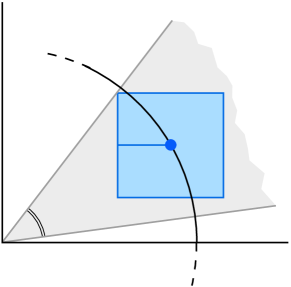
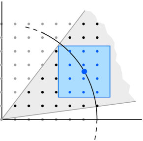
(a)		(b)

Figure 4: Estimation of angle $\phi$ with accuracy $\eta$ (a) is guaranteed when the sine and cosine terms are each estimated with precision $\delta_{\phi}$, where the subscript denotes the dependence on $\phi$; (b) the same estimation based on discrete points during sampling, in this case using 15 samples each for sine and cosine (remaining three orthants omitted).

4.1 Box-based sine and cosine

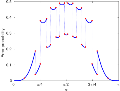
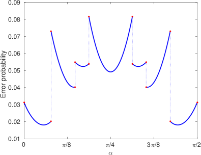
(a)	(b)

Figure 5: Error probability for (a) estimating cosine for different angles for $n=8$ using a bounding box with $\delta=0.3$; (b) error probability for sampling different angles using the wedge-based approach with $n=5$ and $\eta=\pi/4$.

The first sampling method we look at the is box-based scheme discussed in [9, Section 13.5.2] and illustrated in Figure 4(a). The idea is to independently estimate $\cos(2\pi\varphi)$ and $\sin(2\pi\varphi)$ to an accuracy $\eta$, such that the recovered angle differs no more than $\eta$ (in radians) from the actual angle, with probability at least $1-\epsilon$. The following theorem gives the maximum deviation $\delta(\eta)$ allowed in the sine and cosine estimates to reach the desired accuracy in the angle (a proof of the theorem is given in Appendix A):

Theorem 4.1.

For any $0\leq\eta\leq\pi/2$ we can compute an estimate $\tilde{\phi}$ of any $\phi\in[0,2\pi]$ with accuracy $|\tilde{\phi}-\phi|\leq\eta$ from sine and cosine estimates $\tilde{c}$ and $\tilde{s}$ with $|\tilde{c}-\cos(\phi)|\leq\delta$ and $|\tilde{s}-\sin(\phi)|\leq\delta$, whenever

$$\delta\leq\delta(\mbox{$\eta$})=\frac{\sin(\eta)}{\sqrt{2}}.$$ (15)

For uniform estimation over $\phi$ this bound is tight.

Estimating the cosine is equivalent to estimating the probability $p=(1+\cos(2\pi\varphi))/2$ with accuracy $\delta(\eta)/2$. When taking $n$ measurements we can estimate the probability as $k/n$, where $k$ is the number of measurements that are 1. The success set $\mathcal{K}_{n,\delta}(p)$ is therefore defined as

$$\mathcal{K}_{n,\delta}(p):=\{k\in[n]\mid(p-\delta/2)n\leq k\leq(p+\delta/2)n\},$$ (16)

from which we can then evaluate $\mathrm{Pr}(\mathcal{K}_{n,\delta}(p))$. One difficulty here is that the probability $p$ depends on the unknown angle $2\pi\varphi$ and we therefore need to consider the error rate for all possible angles. Figure 5(a) illustrates the error probability $1-\mathrm{Pr}(\mathcal{K}_{n,\delta}(p))$ as a function of angle for $\delta=0.3$, when taking eight measurements. Due to the discrete nature of the samples there are numerous discontinuities, which are best explained using Figure 4(b). Consider the box centered around a point on the circle at a given angle. For the cosine we only need to consider the horizontal component and it may therefore help to think of a projection of the box onto the horizontal axis. Given an angle and corresponding probability $p$, the set $\mathcal{K}_{n,p}$ then consists of all the points on the horizontal axis within the projected box. As the angle increases, the box shifts, thereby gradually adding and removing points from the set $\mathcal{K}$ at critical angles. When looking at the limit as the angle approaches a critical angle, we can take $p$ to be the probability associated with the critical angle. It then follows from (13) that the probability of success increases when a point is added to the set, and decreases when a point is removed, and vice versa for the error rate. Indeed, these discontinuities are clearly seen in the error rate plotted in Figure 5(a). The following theorem, which we prove appendix B, shows that for sufficiently large $n$, the error curve is piecewise convex in $p$:

Theorem 4.2.

Choose $\delta>0$ and let $f_{n}(p)=1-\mathrm{Pr}(X\in\mathcal{K}_{n,\delta}(p))$. Then for $n\geq\max\{1+1/\delta^{2},3\}$, $f_{n}(p)$ is piecewise convex on $[0,1]$ with breakpoints at $[0,1]\cap\{(k/n)\pm\delta/2\}_{k\in[n]}$.

In order to find the maximum error it therefore suffices to evaluate the error function at the critical angles with boundary points removed from $\mathcal{K}_{n,\delta}$. Note that the lower bound on $n$ is a sufficient condition, and Figure 5(a) indicates that the condition on $n$ may be improved or eliminated.

Multi-stage evaluation.

The measurement scheme described in [9] determines $\varphi$ with accuracy $1/16$ and then quantizes to three bits, which adds a maximum deviation of $1/16$, to obtain the desired $1/8$ accurate approximation. Instead of attempting to determine the angle in a single pass, we can also apply the general idea behind Kitaev’s algorithm and use a multi-level approach. For a two-level approach we start with a $1/4$-accurate estimate for $2\varphi$, using $1/8$ accurate angle estimation followed by two-bit quantization $.\overline{\beta^{\prime}_{1}\beta^{\prime}_{2}}$. Based on this, we know that $.\overline{0\beta^{\prime}_{1}\beta^{\prime}_{2}}$ or $.\overline{1\beta^{\prime}_{1}\beta^{\prime}_{2}}$ is a $1/8$ accurate approximation for $\varphi$ and therefore only need to determine the leading bit, which is conveniently done using the phase-shift technique described in Section 3. Even though we quantize the estimation of $2\varphi$ to two bits, we can decide how accurately we want to represent the unquantized estimation, obtained based on the sine and cosine estimates, for use in the phase shift. Using $k\geq 2$ bits gives a maximum deviation of $1/8+1/2^{k+1}$, which, after halving, gives an angle $\pi/8+\pi/2^{k+1}$ for the determination of the sign of the cosine. As shown in Table 1, the smaller the angle the fewer measurements are needed to attain a desired confidence level.

For a three-stage approach we estimate the unquantized angle $4\varphi$ with accuracy $1/4$, and then quantize to a single bit. We then apply two stages of sign determination using a phase shift based on the unquantized angle or a $k$-bit discretization to obtain the final $1/8$ accurate three-bit quantized estimate for $\varphi$.

Angle $/$ $\epsilon$	$10^{-1}$	$10^{-2}$	$10^{-3}$	$10^{-4}$	$10^{-5}$	$10^{-6}$	$10^{-7}$	$10^{-8}$	$10^{-9}$	$10^{-10}$
$7\pi/16$	43	139	247	357	469	583	697	813	927	1043
$6\pi/16$	11	35	61	87	115	143	171	199	227	257
$5\pi/16$	5	15	27	37	49	61	73	85	97	111
$4\pi/16$	3	9	15	21	27	33	39	45	53	59
$3\pi/16$	1	5	9	13	15	19	23	27	31	35
$2\pi/16$	1	3	5	7	9	13	15	17	19	21
$\pi/16$	1	1	3	5	5	7	9	9	11	13
$\pi/32$	1	1	3	3	5	5	7	7	9	9
$\pi/64$	1	1	1	3	3	5	5	5	7	7
$\pi/128$	1	1	1	3	3	3	3	5	5	5
$\pi/256$	1	1	1	1	3	3	3	3	5	5

Table 1: Number of measurement requires to correctly determine the sign of $\cos(\alpha)$ with probability at least $1-\epsilon$, when $\alpha$ deviates from $0$ or $\pi$ by at most the given angle.

Description $/$ $\epsilon$	$10^{-1}$	$10^{-2}$	$10^{-3}$	$10^{-4}$	$10^{-5}$	$10^{-6}$	$10^{-7}$	$10^{-8}$	$10^{-9}$	$10^{-10}$
Single-stage box	112	222	334	452	570	688	806	932	1050	1176
Two-stage box (2-bits)	45	83	121	159	201	241	283	325	365	407
Two-stage box (3-bits)	43	79	115	149	189	225	265	305	343	383
Two-stage box (exact)	43	77	111	145	183	217	255	293	331	369
Three-stage box (2-bits)	52	96	142	190	240	286	336	386	434	484
Three-stage box (3-bits)	38	64	96	126	160	190	224	256	288	320
Three-stage box (exact)	32	54	78	104	130	154	180	208	234	260
Single-stage box, jointly	82	186	296	414	534	652	778	896	1014	1140
Single-stage wedge	40	84	132	188	244	300	358	416	476	534
Two-stage wedge (2-bit)	19	37	57	77	99	119	141	163	185	207
Two-stage wedge (3-bit)	17	33	49	67	87	105	125	145	163	183
Two-stage wedge (exact)	15	29	47	63	81	97	115	133	149	169
Three-stage wedge (2-bit)	30	66	102	138	176	216	254	292	330	368
Three-stage wedge (3-bit)	18	38	58	78	98	122	142	164	184	206
Three-stage wedge (exact)	14	28	42	56	70	88	102	116	132	146
Sign based	15	33	51	69	87	105	123	141	165	183
Sign based (bound)	28	48	68	88	108	128	148	168	188	208
Majority and sign	17	29	41	55	67	79	93	105	119	133
Majority and sign (bound)	22	35	48	62	75	88	102	115	128	141

Table 2: Number of measurements required using different methods to obtain a $1/8$-accurate quantized estimate of $\varphi$ with probability at least $1-\epsilon$.

Numerical evaluation.

We numerically evaluate the different box-based schemes and summarize the number of measurements for different error rates $\epsilon$ in Table 2. For the single-stage measurement scheme we choose $\bar{\epsilon}=\epsilon/2$ to estimate the sine and cosine values. For the two-stage scheme we use $\epsilon/4$ for the sine and cosine estimation and $\epsilon/2$ for the second stage, while for the three-stage scheme we use $\epsilon/6$ for sine and cosine, and $\epsilon/3$ for the last two stages. For each of the instances the condition on $n$ in Theorem 4.2 is satisfied and the numbers reported are therefore optimal for the given setting. Some reduction in the number of measurements in the box-based measurement schemes may however still be obtained by partitioning $\epsilon$ differently over the different stages. The best results are obtained with a three-stage approach, due to the reduction in the number of samples required for the box-based part, as well the limited number of samples needed to accurately determine the sign of the cosine (see Table 1). As a final remark, note that adding more measurements can temporarily increase the error rate due to the discrete nature underlying the error curve. As an example, it can be shown that approximation of the cosine with $\delta=0.1$ succeeds with probability at least $0.7$ for all $n\geq 110$ except $n\in\{113,\ldots,119\}$. Even though these transition regions are not always present, they do show that care needs to be taken when changing the number of samples.

Joint determination of sine and cosine error.

For the box sampling scheme, we determine the number of samples required based on the maximum error probability of the cosine component over all angles. The same number of measurements is then used to independently estimate the sine component. The sine error curve is the same as the cosine error curve, but shifted by $\pi/2$. Based on Figure 5(a) we see that the error probabilities tend to complement, and that joint determination of the error should therefore help reduce the number of measurements. As shown in Table 2 (Single stage box, jointly), this is indeed the case, but the reduction is somewhat modest, and in fact, the reduced number of measurements can be no smaller than that based on the cosine error probability evaluated with $\bar{\epsilon}=\epsilon$ rather than $\epsilon/2$.

4.2 Wedge-based angle

Given $n$ measurements for both $p_{x}=(1+\cos(\alpha))/2$, and $p_{y}=(1+\sin(\alpha))/2$, we can denote by $n_{x}$ and $n_{y}$ the number of 1 measurements. The box-based approach requires that $|{p_{y}-n_{y}/n}|\leq\delta/2$ with high probability, and likewise for $p_{x}$ and $n_{x}/n$. This requirement enables the use of the Chernoff bound to derive a bound on the number of samples, but is otherwise too restrictive. From Figure 4(b) we see that accurate determination of the angle only requires that $(n_{x},n_{y})$ lie within a wedge with angles $\alpha-\eta$ and $\alpha+\eta$ centered at $(n/2,n/2)$. The probability of success then consists of the set of points $\mathcal{K}_{n,\eta}(\alpha)$ within the wedge, which strictly includes the points accepted for the box-based approach. The number of samples required to guarantee a $1-\epsilon$ probability of success will therefore be at least as good or smaller than the box-based approach. (Theoretical results on the error probability in the special case of $\eta=\pi/2$ can be found in [7].)

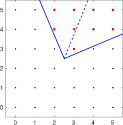
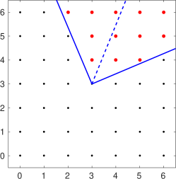
(a) $n=5$	(b) $n=6$

Figure 6: Combinations of sine and cosine measurements that estimate the angle at the center of the wedge with maximum deviation $1/8$.

Numerical evaluation.

Similar to the numerical evaluation of the box approach, in order to find the error rate corresponding to a given number of measurements $n$, we need to minimize $\mathrm{Pr}(\mathcal{K}_{n,\eta}(\alpha))$ over $\alpha$. This can be done by sweeping over the angles $\alpha$, determining $\mathcal{K}_{n,\eta}(\alpha)$ at each point, as illustrated in Figure 6. An example of the resulting error probability for $n=5$ and $\eta=\pi/4$ is shown in Figure 5(b). The break-points in the curve happen at angles where grid points are on the boundary of the wedge (for even $n$, the origin of the wedge $(n/2,n/2)$ is excluded and is therefore not considered to lie on the boundary). The approach therefore is to find all angles $\alpha$ at which the wedge boundary intersects grid points, and evaluate the error probability at those angles, with boundary points at either the bottom or top edges omitted to obtain the limit as $\alpha$ approaches the critical angle from a clockwise or counter-clockwise direction. The error probability in Figure 5(b) appears piecewise convex, but we did not attempt to rigorously establish this. The number of measurements determined using the above algorithm should therefore be interpreted as a lower bound for the method. The resulting number of measurements for the single-stage wedge-based approach, as well as the extension to the two- and three-stage approach described in Section 4.1, are listed in Table 2.

4.3 Triple-sign sampling

When angle $\alpha$ is at most $\pi/4$ from either $0$ or $\pi$, as illustrated in Figure 7(a), the sign-based approach can be used with $p_{x}$ to determine with probability at least $1-\bar{\epsilon}$ whether the point lies on the right or left of the vertical axis. Similarly, when $\alpha$ is $\pi/4$ close to $\pi/2$ or $3\pi/2$, as shown in Figure 7(b), we can tell with the same probability whether the point lies above or below the horizontal axis. When $\alpha$ lies outside of the given range we make no assumption on the results in either case. When applying both schemes we can combine the obtained signs, as shown in Figure 7(c). By construction we know that at least one of the two is correct, up to the desired success rate of $1-\bar{\epsilon}$. For angles between $\pi/4$ and $3\pi/4$, as illustrated in the plot, this means that when the method succeeds we obtain either $01$ or $11$. The maximum error obtained in this case is therefore $\pi/2$. A more convenient quantization can be obtained by applying a phase shift of $\pi/4$ prior to applying the two measurement steps, followed by the inverse phase shift to the result. After changing the labels we obtain the quantization values given in Figure 7(d). To obtain a $1/8$ accurate estimation we can apply an additional Kitaev step with sign-based sampling.

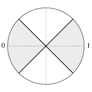
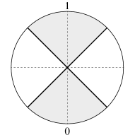
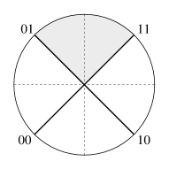
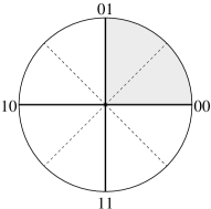
(a)	(b)	(c)	(c)

Figure 7: Estimation of (a) the horizontal and (b) the vertical component of the angle, accurate for angles in the shaded regions; (c) combination of the two sign-based estimates to obtain a $1/4$ accurate quantization; and (d) alternative quantization obtained by applying a $\pi/4$ rotation before the measurements and an inverse rotation and relabeling afterwards.

For the sufficient number of measurements per component, Theorem 3.1 applied with $\alpha=\pi/4$ gives

$$n\geq\frac{\log(1/\epsilon)}{\log(1/\sin(\pi/4))}=\frac{\log(1/\epsilon)}{\log(2/\sqrt{2})}=\frac{\log(1/\epsilon)}{\log(2)-\log(2)/2}=2\log_{2}(1/\epsilon).$$ (17)

The first stage requires $n$ measurements each for the horizontal and vertical component. The second stage requires another $n$ measurements, for a total of $3n$ measurements. For each of the three steps we can choose $\bar{\epsilon}=\epsilon/2$ for a total maximum error of $\epsilon$. Note that the maximum error in the first stage is $\bar{\epsilon}$, since one of the two components is irrelevant (although we do not know which of the two it is). Combined we can take

$$N=3\lceil 2\log_{2}(2/\epsilon)\rceil\leq 9+6\log_{2}(1/\epsilon),$$ (18)

where the inequality is due to the addition of 3 to account for rounding to integers.

4.4 Majority sampling

$.\overline{01}$
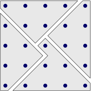
$.\overline{10}$ $.\overline{00}$		$j\!=\!0$ $\ldots$ $n$
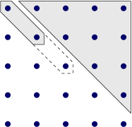
$.\overline{11}$			$i=0$ $\ldots$ $n$
(a)	(b)		(c)

Figure 8: Classification regions for majority-based sampling for (a) odd, and (b) even $n$; and (c) the success set $\mathcal{K}_{n}$ for angles in the range $[0,\pi/2)$.

For majority sampling we take $n$ measurements for the sine and cosine components, and count the number of positive measurements by $n_{y}$ and $n_{x}$, respectively. The quantized approximation of the angle is defined in terms of the majority of the number of 0 or 1 measurements

$$q(n_{x},n_{y})=\begin{cases}.\overline{00}&n_{x}\geq\max\{n_{y},n-n_{y}+1\}\\ .\overline{01}&n_{y}\geq\max\{n_{x}+1,n-n_{x}\}\\ .\overline{10}&n-n_{x}\geq\max\{n_{y}+1,n-n_{y}\}\\ .\overline{11}&\mathrm{otherwise},\end{cases}$$

which gives partitions as illustrated in Figures 8(a) and (b). We want to obtain an estimator that is 1/4 accurate with probability at least $1-\epsilon$. In particular we allow angles $\phi\in[0,1/4)$ to be quantized as either $.\overline{00}$ or $.\overline{01}$, and similarly for interval increments of $1/4$. Denoting by $\mathcal{K}_{ab}$ the set of points that map to $.\overline{ab}$, this gives a success set of $\mathcal{K}_{00}\cup\mathcal{K}_{01}$. For the analysis of the error we work with a reduced set $\mathcal{K}_{n}=\{(i,j)\mid i,j\in[0,n],j\geq n-i+1\}$, illustrated by the top-right triangle in Figure 8(c). Based on this we have the following result (proven in Appendix C):

Theorem 4.3.

Let $\mathcal{K}_{n}=\{(i,j)\mid i,j\in[0,n],j\geq n-i+1\}$, then for all $\alpha\in[0,\pi/2]$

$$1-\mathrm{Pr}(\mathcal{K}_{n}\mid n,\alpha)\leq\frac{2}{2^{n}}.$$

We expect that this result can be improved by a factor of two. Indeed, defining the error probability

$$f_{n}(\alpha)=1-\mathrm{Pr}(\mathcal{K}_{n}\mid n,\alpha)$$ (19)

over angles $\alpha=2\pi\varphi$, it can be seen from Figure 9 that the error curves are convex and attain the maximum at $\alpha=0$. The error probability is the summation of the probabilities for $(i,j)\not\in\mathcal{K}_{n}$. At $\alpha=0$, we have $p_{x}=1$, which implies that all terms including $(1-p_{x})^{n-i}$ are zero, except those with $i=n$. The only such point is $(n,0)$, and we therefore have

$$f_{n}(0)=(1-p_{y})^{n}=(1-\textstyle\frac{1}{2})^{n}=2^{-n}.$$

We can now expand $\mathcal{K}_{n}$ with any of the points in the gray part of the diagonal in Figure 8(c). This lowers the error for $\alpha>0$ but does not affect $f_{n}(0)$. Under the assumption that the maximum of $f_{n}(\alpha)$ is attained at $\alpha=0$, the maximum error for the set $\mathcal{K}_{00}\cup\mathcal{K}_{01}$ is therefore $2^{-n}$. By rotational symmetry the same applies for the remaining quadrants, including the special case of $\mathcal{K}_{11}$ for even $n$. Extending $\mathcal{K}_{n}$ only decreases the error and the result in Theorem 4.3 continues to hold. The error probability for the majority-based approach over all angles is therefore bounded by $2/2^{n}$, which can likely be improved to $1/2^{n}$. The approach requires $n$ samples in both the horizontal and vertical direction therefore amounting to a total of $N=2n$ samples. In order to achieve an accuracy of $1/8$, we combine the majority-based approach with a single stage of sign determination. The resulting number of samples for different values of $\epsilon$ is listed in Table 2. A theoretical bound on the number of samples can be found using (17), giving

$$N=2\lceil\log_{2}(4/\epsilon)\rceil+\lceil 2\log_{2}(2/\epsilon)\rceil\leq 9+4\log_{2}(1/\epsilon).$$

This bound can be lowered by two samples if it can be shown that $\alpha=0$ maximizes $f_{n}(\alpha)$ over $[0,\pi/2]$.

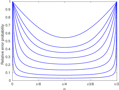
Figure 9: Error probability $f_{n}(\alpha)$ scaled by $2^{n}$, with from top to bottom $n=1,2,3,5,10,25,100,500$.

5 Evaluation of $N_{\epsilon}$

For a given $\epsilon$ we can first determine $k_{\epsilon}$ using (12) and set $\bar{\epsilon}=\epsilon/k_{\epsilon}$. Denote by $N_{k}$ the number of samples in steps $k=1,\ldots,k_{\epsilon}-1$. For the first step we can either use the triple-sign ($s$) or majority ($m$) based approaches giving respectively

$$N_{1}^{s}=9+6\log_{2}(1/\bar{\epsilon}),\quad\mathrm{or}\quad N_{1}^{m}=9+4\log_{2}(1/\bar{\epsilon}).$$ (20)

For the remaining steps we use the sign-based approach with angles $\alpha=\pi/2^{k+1}$. Using Theorem 3.1, and ignoring rounding up to the nearest integer we can take

$$N_{k}=\frac{\log(1/\bar{\epsilon})}{\log(1/\sin(\pi/2^{k+1}))}\leq\frac{\log(1/\bar{\epsilon})}{\log(2^{k-1})}=\frac{\log_{2}(1/\bar{\epsilon})}{k-1},$$

where the inequality follows from $\sin(\pi/2^{k+1})\leq\pi/2^{k+1}\leq 4/2^{k+1}=1/2^{k-1}$. Summing over $N_{k}$ gives

$$\sum_{k=2}^{k_{\epsilon}-1}N_{k} = \log_{2}(1/\bar{\epsilon})\sum_{k=1}^{k_{\epsilon}-2}\frac{1}{k}$$ (21)

$$\leq \log_{2}(1/\bar{\epsilon})\left(1+\int_{1}^{k_{\epsilon}-2}x^{-1}dx\right)$$

$$= \log_{2}(1/\bar{\epsilon})\left(1+\log(k_{\epsilon}-2)\right)$$

To account for rounding up of the intermediate values we add one for each of the remaining $k_{\epsilon}-2$ steps. Combining (20), (21), and the rounding term, and using $\log_{2}(1/\bar{\epsilon})=\log_{2}(1/\epsilon)+\log_{2}(k_{\epsilon})$ gives

$$N_{\epsilon}^{s}\leq 7+k_{\epsilon}+(7+\log(k_{\epsilon}-2))\cdot(\log_{2}(1/\epsilon)+\log_{2}(k_{\epsilon}))$$ (22)

for triple-sign based sampling and

$$N_{\epsilon}^{m}\leq 7+k_{\epsilon}+(5+\log(k_{\epsilon}-2))\cdot(\log_{2}(1/\epsilon)+\log_{2}(k_{\epsilon}))$$ (23)

for majority-based sampling.

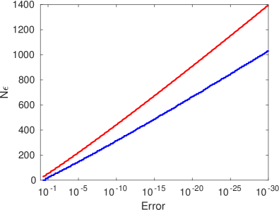
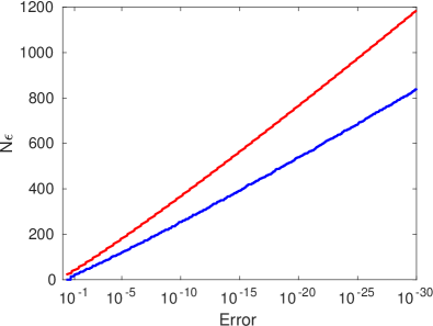
(a)	(b)

Figure 10: Numerical evaluation of $N_{\epsilon}$ along with the theoretical upper bound, using (a) triple-sign sampling, and (b) majority-based sampling.

Numerical evaluation.

For a numerical evaluation of $N_{\epsilon}$ we first determine the critical iteration $k_{\epsilon}$ by finding the smallest integer $k$ that satisfies (11). Based on $k_{\epsilon}$ we set $\bar{\epsilon}=\epsilon/k_{\epsilon}$ and use both the triple-sign and majority-based sampling methods for the first iteration. After that we use sign-based sampling with increasingly accurate phase shifts to obtain the total number of evaluations before reaching iteration $k_{\epsilon}$. The resulting values for $N_{\epsilon}$ are plotted in Figure 10 along with the theoretical bounds given in equations (22) and (23). A summary of $k_{\epsilon}$ for different values of $\epsilon$ as well as $N_{\epsilon}$ values for the two different sampling methods used in the first iteration is given in Table 4. Finally, Table 4 gives the total number of iterations needed to obtain a $2^{-(m+2)}$ accurate phase estimate with probability at least $1-\epsilon$ up to and including iteration $k_{\epsilon}$. For each combination of $\epsilon$ and $m$ that contains a number, we choose $\bar{\epsilon}=\epsilon/m$. The dashed fields are in the regime where a single measurement can be taken per additional bit of the estimated angle, without having to change $\bar{\epsilon}$.

Description $\backslash$ $\epsilon$	$10^{-1}$	$10^{-2}$	$10^{-3}$	$10^{-4}$	$10^{-5}$	$10^{-6}$	$10^{-7}$	$10^{-8}$	$10^{-9}$	$10^{-10}$
$k_{\epsilon}$ using (11)	3	5	7	9	10	12	14	16	17	19
$k_{\epsilon}$ using (12)	4	6	7	9	11	12	14	16	17	19
$N_{\epsilon}^{s}$ (triple-sign)	24	56	84	116	147	177	213	243	280	314
$N_{\epsilon}^{s}$ (triple-sign, bound (22))	44	84	123	163	197	237	277	317	353	394
$N_{\epsilon}^{m}$ (majority)	24	48	72	96	121	147	175	199	226	256
$N_{\epsilon}^{m}$ (majority, bound (23))	34	66	98	130	158	190	223	256	285	319

Table 3: Summary of $k_{\epsilon}$ for different values of $\epsilon$ as well as $N_{\epsilon}$ values for different sampling methods.

Triple-sign sampling
$\epsilon$ $\backslash$ $m$	$1$	$2$	$3$	$4$	$5$	$6$	$7$	$8$	$9$	$10$	$11$	$12$	$13$	$14$	$15$	$16$	$17$	$18$	$19$
$10^{-1}$	15	16	19	–	–	–	–	–	–	–	–	–	–	–	–	–	–	–	–
$10^{-2}$	33	36	41	42	45	–	–	–	–	–	–	–	–	–	–	–	–	–	–
$10^{-3}$	51	58	61	66	69	70	73	–	–	–	–	–	–	–	–	–	–	–	–
$10^{-4}$	69	78	83	86	89	94	97	98	99	–	–	–	–	–	–	–	–	–	–
$10^{-5}$	87	98	105	110	113	116	119	122	127	130	–	–	–	–	–	–	–	–	–
$10^{-6}$	105	118	125	132	137	140	145	150	153	156	159	160	–	–	–	–	–	–	–
$10^{-7}$	123	138	147	154	161	166	169	172	175	178	183	186	189	190	–	–	–	–	–
$10^{-8}$	141	158	169	178	185	190	195	198	203	206	209	212	215	218	219	220	–	–	–
$10^{-9}$	165	184	199	208	215	220	225	230	233	236	239	242	245	248	251	254	257	–	–
$10^{-10}$	183	206	219	228	235	242	247	252	259	264	267	272	275	278	281	284	287	290	291
Majority-based sampling
$\epsilon$ $\backslash$ $m$	$1$	$2$	$3$	$4$	$5$	$6$	$7$	$8$	$9$	$10$	$11$	$12$	$13$	$14$	$15$	$16$	$17$	$18$	$19$
$10^{-1}$	17	20	25	–	–	–	–	–	–	–	–	–	–	–	–	–	–	–	–
$10^{-2}$	29	34	43	44	49	–	–	–	–	–	–	–	–	–	–	–	–	–	–
$10^{-3}$	41	50	57	62	69	70	73	–	–	–	–	–	–	–	–	–	–	–	–
$10^{-4}$	55	68	73	80	83	88	93	96	97	–	–	–	–	–	–	–	–	–	–
$10^{-5}$	67	82	91	98	101	106	109	114	119	122	–	–	–	–	–	–	–	–	–
$10^{-6}$	79	96	107	114	121	124	131	136	141	144	147	148	–	–	–	–	–	–	–
$10^{-7}$	93	112	123	132	139	146	151	154	157	160	167	170	173	176	–	–	–	–	–
$10^{-8}$	105	126	141	150	159	166	171	174	181	184	189	192	195	198	199	200	–	–	–
$10^{-9}$	119	142	159	170	179	184	189	196	201	204	207	210	213	216	219	224	227	–	–
$10^{-10}$	133	160	173	186	193	200	209	214	221	226	229	234	239	244	247	250	253	256	257

Table 4: Number of samples required to obtain an $2^{-(m+2)}$ accurate estimation of $\varphi$ with probability at least $1-\epsilon$ using triple-sign based sampling (top) and majority-based sampling (bottom). Dashed lines indicate the regime where a single extra measurement is needed for each successive $m$.

6 Discussion

In this work we have proposed and analyzed several sampling schemes for use in quantum phase estimation based on Kitaev’s algorithm, and showed that using previous phase estimates to shift the phase can reduce the number of measurements. Based on this we showed in Section 3 that we can obtain a theoretical sampling complexity $N_{\epsilon}+m$ to obtain a $2^{-(m+2)}$ accurate estimation of the phase $\varphi$ with probability at least $\epsilon$. The proposed approach requires increasingly accurate rotations, which may not be feasible in practice due to inherent system noise or circuit complexity (see [17] for the implementation of small rotations). Even with practical limitations on the phase shift accuracy, as studied in more detail in [1], the proposed sampling schemes can still reduce the number of measurements, as shown, for example, in Table 1. From a theoretical point of view, having a limited accuracy re-introduces a $\log(m)$ dependency in the algorithmic complexity, and it will therefore be interesting to analyze the application of the sampling schemes to the phase estimation algorithm proposed in [14]. Another potential minor drawback of our approach is the dependency of each iteration relies on the outcome of the previous one, thereby limiting the potential parallelism to the independent measurements within each iteration.

It remains to show that the maximum of $f_{n}(\alpha)$ in (19) over $[0,\pi/2]$ is attained at $\alpha=0$. This would confirm a sampling complexity of $2\log_{2}(1/\epsilon)$ for the majority-based approach. This was verified for $n=1$ and $n=2$, and Figure 9 strongly suggests this holds for all $n$. Indeed, for $n=1$ we have

$$f_{1}(\alpha)=(1-\sin(\alpha)-\cos(\alpha)-\sin(\alpha)\cos(\alpha))/4,$$

which is convex over the given range due to concavity of the trigonometric terms, and the result therefore follows from the symmetry $f_{n}(\alpha)=f_{n}(\pi/2-\alpha)$. Empirically, the error functions for box-, wedge-, and majority-based sampling all exhibit convexity or piecewise convexity. This may indicate a more general relationship between the error over certain index sets $\mathcal{K}$ and $\alpha$.

Appendix A Proof of Theorem 4.1

Theorem 4.1.

For any $0\leq\eta\leq\pi/2$ we can compute an estimate $\tilde{\phi}$ of any $\phi\in[0,2\pi]$ with accuracy $|\tilde{\phi}-\phi|\leq\eta$ from sine and cosine estimates $\tilde{c}$ and $\tilde{s}$ with $|\tilde{c}-\cos(\phi)|\leq\delta$ and $|\tilde{s}-\sin(\phi)|\leq\delta$, whenever

$$\delta\leq\delta(\phi)=\frac{\sin(\eta)}{\sqrt{2}}.$$ (24)

For uniform estimation over $\phi$ this bound is tight.

Proof.

For $\eta=0$ the result holds trivially with $\delta=0$, and we therefore only need to consider $\eta>0$. We can recover any $\phi$ with accuracy $\eta$ from approximate sine and cosine values $\tilde{c}$ and $\tilde{s}$ if and only if $(\tilde{c},\tilde{s})$ lies within a wedge of angles between $\phi-\eta$ and $\phi+\eta$ (illustrated by the shaded region in Figure 4). For $\delta$, this means that the square with sides $2\delta$ centered on $\phi$ must to lie within the wedge. For $0<\eta\leq\pi/4$ we can assume without loss of generality that $\phi\in[0,\pi/4]$. It can be seen that the intersection of the top-left corner of the box, at $(\cos(\phi)-\delta,\sin(\phi)+\delta)$, with the boundary of the wedge at angle $\phi+\eta$ determines the maximum value of $\delta$. Formalizing, we write $\delta(\phi)$ to indicate the dependence on $\phi$ and denote the wedge boundary as $x=\alpha(\phi)y$, with

$$\alpha(\phi)=\frac{\cos(\phi+\eta)}{\sin(\phi+\eta)}.$$

For $\delta$ to be valid we need $\cos(\phi)-\delta\geq\alpha(\phi)(\sin(\phi)+\delta)$, which can be rewritten as

$$\delta\leq\delta(\phi)=\frac{\cos(\phi)-\alpha(\phi)\sin(\phi)}{1+\alpha(\phi)}$$ (25)

We then need to minimize $\delta(\phi)$ over the given range of $\phi$ to find the largest value of $\delta$ that applies for all $\phi$. Abbreviating $\alpha=\alpha(\phi)$ and gradient $\alpha^{\prime}=\alpha^{\prime}(\phi)$, we have

$$\delta^{\prime}(\phi) = -\frac{\sin(\phi)}{1+\alpha}-\frac{\alpha\cos(\phi)}{1+\alpha}-\frac{\alpha^{\prime}\cos(\phi)}{(1+\alpha)^{2}}-\sin(\phi)\left(\frac{\alpha^{\prime}}{1+\alpha}-\frac{\alpha\alpha^{\prime}}{(1+\alpha)^{2}}\right)$$ (26)

$$= -\sin(\phi)\left(\frac{1}{1+\alpha}+\frac{\alpha^{\prime}}{(1+\alpha)^{2}}\right)-\cos(\phi)\left(\frac{\alpha}{1+\alpha}+\frac{\alpha^{\prime}}{(1+\alpha)^{2}}\right)$$

From

$$\alpha^{\prime}=-\frac{1}{\sin^{2}(\phi-\eta)},\quad\mbox{and}\quad\alpha^{2}=\frac{\cos^{2}(\phi+\eta)}{\sin^{2}(\phi+\eta)}=\frac{1-\sin^{2}(\phi+\eta)}{\sin^{2}(\phi+\eta)}=\frac{1}{\sin^{2}(\phi+\eta)}-1,$$

it follows that $\alpha^{\prime}+\alpha^{2}=-1$, or $\alpha^{\prime}=-1-\alpha^{2}$, which allows us to simplify the sine coefficient as

$$\frac{1}{1+\alpha}+\frac{\alpha^{\prime}}{(1+\alpha)^{2}}=\frac{1+\alpha}{(1+\alpha)^{2}}-\frac{1+\alpha^{2}}{(1+\alpha)^{2}}=\frac{\alpha(1-\alpha)}{(1+\alpha)^{2}},$$ (27)

whereas for the cosine coefficient we find

$$\frac{\alpha}{1+\alpha}+\frac{\alpha^{\prime}}{(1+\alpha)^{2}}=\frac{\alpha+\alpha^{2}+\alpha^{\prime}}{(1+\alpha)^{2}}=\frac{(\alpha-1)}{(1+\alpha)^{2}}.$$ (28)

Substituting (27) and (28) in (26) gives

$$\delta^{\prime}(\phi)=\cos(\phi)\frac{(1-\alpha)}{(1+\alpha)^{2}}-\alpha\sin(\phi)\frac{(1-\alpha)}{(1+\alpha)^{2}}.$$ (29)

Noting that $\eta>0$ and considering the range of $\phi$, we have $0<\sin(\phi+\eta)\leq 1$. This allows us to multiply the first term in (29) by $\sin(\phi+\eta)/\sin(\phi+\eta)$, and expand the enumerator in this term using the sum formula as

$$\sin(\phi+\eta)=\sin(\phi)\cos(\eta)+\cos(\phi)\sin(\eta).$$

Finally, expanding the enumerator $\cos(\phi+\eta)$ in the $\alpha$ term preceding $\sin(\phi)$ as

$$\cos(\phi+\eta)=\cos(\phi)\cos(\eta)-\sin(\phi)\sin(\eta),$$

and simplifying gives

$$\delta^{\prime}(\phi)=\frac{(1-\alpha)}{(1+\alpha)^{2}\sin(\phi+\eta)}\sin(\eta).$$ (30)

All terms in this expression, except $\alpha-1$, are strictly positive. The gradient is therefore zero only when $\alpha=1$, which happens at $\phi^{*}=\pi/4-\eta$. For $\phi<\phi^{*}$ we have $\alpha(\phi)>1$ and therefore $\delta^{\prime}(\phi)<0$, whereas for $\phi>\phi^{*}$ we have $\alpha(\phi)<1$ and $\delta^{\prime}(\phi)>0$, which shows that $\phi^{*}$ gives a minimizer. Evaluating $\delta(\phi^{*})$ in (25) and noting that $\alpha(\phi^{*})=1$ then gives

$$\delta\leq\delta(\phi)=(\cos(\pi/4-\eta)-\sin(\pi/4-\eta))/2.$$

To obtain the desired result, we simplify $\delta(\phi)$ using the sum formulas and $\cos(\pi/4)=\sin(\pi/4)=\sqrt{2}/2$:

$$\delta(\phi) = \frac{1}{2}\left((\cos(\pi/4)\cos(\eta)+\sin(\pi/4)\sin(\eta))-(\sin(\pi/4)\cos(\eta)-\cos(\pi/4)\sin(\eta))\right)$$

$$= \frac{\sqrt{2}}{4}\left((\cos(\eta)+\sin(\eta))-(\cos(\eta)-\sin(\eta))\right)=\frac{1}{\sqrt{2}}\sin(\eta).$$

For $\pi/4\leq\eta\leq\pi/2$ we can assume without loss of generality that $\phi\in[-\pi/4,0]$. In this case the top-left corner of the box can again be seen to limit $\delta$. The argument as given above follows through as is, thus completing the proof. ∎

Appendix B Proof of Theorem 4.2

Theorem 4.2.

Choose $\delta>0$ and let $f_{n}(p)=1-\mathrm{Pr}(X\in\mathcal{K}_{n,\delta}(p))$ with $\mathcal{K}_{n,p}$ as defined in (16). Then for $n\geq\max\{1+1/\delta^{2},3\}$, $f_{n}(p)$ is piecewise convex on $[0,1]$ with breakpoints at $[0,1]\cap\{(k/n)\pm\delta/2\}_{k\in[n]}$.

Proof.

From the definition of $\mathcal{K}_{n,\delta}(p)$, it is clear that $\mathcal{K}_{n,\delta}(p)$ remains constant precisely on the (open) segment between the stated breakpoints. Choose any segment, then for all values of $p$ within this segment, the error is obtained by summing $B(k;n,p)$ over $k\not\in\mathcal{K}_{n,\delta}(p)$, with

$$B(k;n,p)={n\choose k}p^{k}(1-p)^{n-k}.$$

In order to prove convexity of the error over the segment, we show that the each of the terms $B(k;n,p)$ is convex in $p$ over the segment. For conciseness we normalize with respect to the binomial coefficient and work with $B_{k,n}(p):=B(k;n,p)/{n\choose k}$. For $n=2$, observe that the second derivative $B_{1,2}^{\prime\prime}(p)=-2$ is negative, which means that $B_{1,2}(p)$ is concave. We therefore require that $n\geq 3$. For $k=0$ and $k=n$ we find

$$B_{0,n}^{\prime\prime}(p)=n(n-1)(1-p)^{n-2},\quad\mathrm{and}\quad B_{n,n}^{\prime\prime}(p)=n(n-1)p^{n-2}.$$

The second derivatives are nonnegative over the domain $p\in[0,1]$ and the functions are therefore convex. For $0<k<n$ we have

$$B_{k,n}^{\prime}(p) = (k(1-p)-(n-k)(p))(p^{k-1}(1-p)^{n-k-1})$$ (31)

$$= (k-np)\left(p^{k-1}(1-p)^{n-k-1}\right),$$

and the gradient reaches zero when $p=0$, $p=1$, or $p=k/n$. For $k=1$ we find

$$B_{1,n}^{\prime\prime}(p) = \left[-n(1-p)-(1-np)(n-2)\right](1-p)^{n-3}$$

$$= \left[np(n-1)-2(n-1)\right](1-p)^{n-3}$$

For convexity we want $B_{1,n}^{\prime\prime}(p)\geq 0$, and therefore require that the square-bracketed term be nonnegative. Solving for $p$ then gives convexity of $B_{1,n}(p)$ for $p\geq 2/n$. By symmetry, it follows that for $k=n-1$, $B_{{n-1},n}(p)$ is convex for $p\leq 1-2/n$. Finally, for $2\leq k\leq n-2$ it follows from (31) that

$$B^{\prime\prime}_{k,n}(p) = \left(-np(1-p)+(k-np)\left((k-1)(1-p)-(n-k-1)p\right)\right)\cdot\left(p^{k-2}(1-p)^{n-k-2}\right)$$

$$= \left[n(n-1)p^{2}-2k(n-1)p+k(k-1)\right]\cdot\left(p^{k-2}(1-p)^{n-k-2}\right).$$

The term in square brackets is a quadratic in $p$, and solving for the roots gives

$$p_{\pm}=\frac{k}{n}\pm\frac{\sqrt{k(n-1)(n-k)}}{n(n-1)}.$$

The deviation is maximum at $k=n/2$, which gives

$$\frac{\sqrt{k(n-1)(n-k)}}{n(n-1)}\leq\frac{(n/2)\sqrt{n-1}}{n(n-1)}=\frac{1}{2\sqrt{n-1}}.$$

The second derivative $B_{k,n}^{\prime\prime}$ is therefore guaranteed to be nonnegative, and $B_{k,n}$ convex, when $p$ is at least $1/(2\sqrt{n-1})$ away from the maximum at $k/n$. It can be verified that the same sufficient condition applies for $k=0$ and $k=n$.

For any $p$ in the selected segment we know that $\mathcal{K}_{n,\delta}(p)$ remains constant and that $|{k/n-p}|\geq\delta/2$ for any $k\not\in\mathcal{K}_{n,\delta}(p)$. To guarantee convexity we therefore require that

$$\delta/2\geq 1/(2\sqrt{n-1}),$$

which simplifies to $n\geq 1+1/\delta^{2}$. ∎

Appendix C Proof of Theorem 4.3

Theorem 4.3.

Let $\mathcal{K}_{n}=\{(i,j)\mid i,j\in[0,n],j\geq n-i+1\}$, then for all $\alpha\in[0,\pi/2]$

$$1-\mathrm{Pr}(\mathcal{K}_{n}\mid n,\alpha)\leq\frac{2}{2^{n}}.$$

Proof.

Denote by $\mathcal{E}_{n}=\{(i,j)\mid i,j\in[0,n],i+j\leq n\}$ the complement of $\mathcal{K}_{n}$. The error probability $\mathrm{Pr}(\mathcal{E}_{n}\mid n,\alpha)=1-\mathrm{Pr}(\mathcal{K}_{n}\mid n,\alpha)$ is then obtained by summing $f_{i,j}$ over $(i,j)\in\mathcal{E}_{n}$, where

$$f_{i,j}(\alpha)={n\choose i}{n\choose j}p_{x}^{i}(1-p_{x})^{n-i}p_{y}^{j}(1-p_{y})^{n-j}.$$

Defining the diagonal sums $k\in[0,n]$ as

$$d_{k}(\alpha)=\sum_{i=0}^{k}f_{i,k-j}(\alpha),$$

we can equivalently write $\mathrm{Pr}(\mathcal{E}_{n}\mid n,\alpha)=\sum_{k=0}^{n}d_{k}(\alpha)$. For $\alpha\in[0,\pi/2]$ it is easily seen that $d_{k}(\alpha)=d_{k}(\pi/2-\alpha)$, and it therefore suffices to show the desired result for $\alpha\in[0,\pi/4]$. As a first step, we bound the value of the main diagonal $d_{n}$ by $2^{-n}$:

$$d_{n}(\alpha) = \sum_{j=0}^{n}{n\choose n-j}{n\choose j}p_{x}^{n-j}(1-p_{x})^{j}p_{y}^{j}(1-p_{y})^{n-j}$$

$$= (p_{x}(1-p_{y}))^{n}\sum_{j=0}^{n}{n\choose j}^{2}\left(\frac{p_{y}(1-p_{x})}{p_{x}(1-p_{y})}\right)^{j}$$

$$= (p_{x}(1-p_{y}))^{n}\sum_{j=0}^{n}\left({n\choose j}\left(\frac{p_{y}(1-p_{x})}{p_{x}(1-p_{y})}\right)^{j/2}\right)^{2}$$

$$\leq (p_{x}(1-p_{y}))^{n}\left(\sum_{j=0}^{n}{n\choose j}\left(\frac{\sqrt{p_{y}(1-p_{x})}}{\sqrt{p_{x}(1-p_{y})}}\right)^{j}\right)^{2}$$

$$\stackrel{{\scriptstyle(i)}}{{=}} (p_{x}(1-p_{y}))^{n}\left(1+\frac{\sqrt{p_{y}(1-p_{x})}}{\sqrt{p_{x}(1-p_{y})}}\right)^{2n}$$

$$\stackrel{{\scriptstyle(ii)}}{{=}} (p_{x}(1-p_{y}))^{n}\left(\frac{1}{2p_{x}(1-p_{y})}\right)^{n}$$

$$= 2^{-n},$$

where (i) uses the binomial theorem and (ii) follows from the observation that

$$\left(1+\frac{\sqrt{p_{y}(1-p_{x})}}{\sqrt{p_{x}(1-p_{y})}}\right)^{2} = \left(\frac{\sqrt{p_{x}(1-p_{y})}+\sqrt{p_{y}(1-p_{x})}}{\sqrt{p_{x}(1-p_{y})}}\right)^{2}$$

$$= \frac{p_{x}(1-p_{y})+2\sqrt{p_{x}(1-p_{x})p_{y}(1-p_{y})}+p_{y}(1-p_{x})}{p_{x}(1-p_{y})}$$

$$\stackrel{{\scriptstyle\eqref{Eq:4p(1-p)}}}{{=}} \frac{p_{x}(1-p_{y})+2\sqrt{\sin^{2}(\alpha)\cos^{2}(\alpha)/16}+p_{y}(1-p_{x})}{p_{x}(1-p_{y})}$$

$$= \frac{(1+\cos(\alpha)(1-\sin(\alpha))/4+\sin(\alpha)\cos(\alpha)/2+(1+\sin(\alpha))(1-\cos(\alpha))/4}{p_{x}(1-p_{y})}$$

$$= \frac{1}{2p_{x}(1-p_{y})}.$$

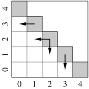
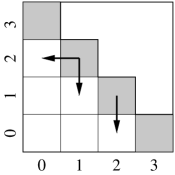
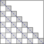
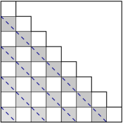
(a)	(b)	(c)	(d)

Figure 11: Constructions for bounding (a,b) $d_{n-1}$ based on $d_{n}$, and (c,d) the sum of $d_{k}$ for strided $k$.

For the second step we derive a bound on $d_{n-1}$ based on $d_{n}$, from which we then obtain a bound on $d_{n-1}+d_{n}$. For $i\geq 1$ we have

$$f_{i-1,j}=f_{i,j}\cdot\frac{1-p_{x}}{p_{x}}\cdot\frac{i}{n-i+1}.$$

The right-most term, which accounts for the change in the binomial coefficient ${n\choose i}$, is less than or equal to 1 for $i\leq n/2$ when $n$ is even, and for $i\leq(n+1)/2$ when $n$ is odd. A similar argument applies for the transition from $f_{i,j}$ to $f_{i,j-1}$ for $1\leq j\leq(n+1)/2$, allowing us to bound the elements on the $(n-1)$-diagonal $d_{n-1}$ as follows:

$$f_{i,j}\leq\begin{cases}\displaystyle\frac{1-p_{x}}{p_{x}}f_{i+1,j}&i<(n-1)/2,\\[14.0pt] \displaystyle\frac{1-p_{y}}{p_{y}}f_{i,j+1}&\mathrm{otherwise}.\end{cases}$$

As illustrated in Figures 11(a) and (b), this approach uses the middle element of the main diagonal twice. Taking this into account, and effectively doing the same for all elements, we have

$$d_{n-1}\leq\left(\frac{1-p_{x}}{p_{x}}+\frac{1-p_{y}}{p_{y}}\right)d_{n}=\frac{p_{y}(1-p_{x})+p_{x}(1-p_{y})}{p_{x}p_{y}}d_{n}.$$ (33)

Combining (C) and (33) we have

$$d_{n}+d_{n-1}\leq\frac{p_{x}+p_{y}-p_{x}p_{y}}{p_{x}p_{y}}\cdot 2^{-n}.$$ (34)

As the third step, we derived bound on $d_{k-2}$ based on $d_{k}$. Consider any diagonal $2\leq k\leq n$, with $0<i<k$ and $j=k-i$, then

$${n\choose i-1}{n\choose j-1}={n\choose i-1}{n\choose k-i-1}=\frac{i}{n-i+1}\cdot\frac{k-i}{n-k+i+1}{n\choose i}{n\choose k-i}=\kappa{n\choose i}{n\choose j}$$

Since $k\leq n$, the multiplicative term $\kappa$ satisfies

$$\kappa=\frac{i(k-i)}{i(k-i)+n(n-k+1)-k+2}\leq\frac{i(k-i)}{i(k-i)+n-k+2}\leq\frac{i(k-i)}{i(k-i)+2}<1.$$

It therefore follows that

$$f_{i-1,k-i-1}\leq f_{i,k-i}\cdot\frac{(1-p_{x})}{p_{x}}\cdot\frac{(1-p_{y})}{p_{y}}.$$

The transition from diagonal $k$ to $k-2$ follows by summing over all elements $i+j=k-2$, giving

$$d_{k-2}\leq\frac{(1-p_{x})(1-p_{y})}{p_{x}p_{y}}d_{k}=\tau d_{k},$$

with $\tau<1$, as shown in Figure 12(a). As a fourth step we sum over the even and odd diagonals. Starting at $k=n$ or $k=n-1$ we have

$$\sum_{i=0}^{k/2}d_{k-2i}\leq\sum_{i=0}^{\infty}\tau^{i}d_{k}=\frac{1}{1-\tau}d_{k}=\frac{p_{x}p_{y}}{p_{x}+p_{y}-1}\cdot d_{k}$$

For the sum of the diagonals, and hence that $f_{i,j}$ over the error set set $\mathcal{E}_{n}$, it follows from (34) that

$$\sum_{k=0}^{n}d_{k}\leq\frac{p_{x}p_{y}}{p_{x}+p_{y}-1}(d_{n}+d_{n-1})\leq\frac{p_{x}p_{y}}{p_{x}+p_{y}-1}\cdot\frac{p_{x}+p_{y}-p_{x}p_{y}}{p_{x}p_{y}}\cdot 2^{-n}=\frac{p_{x}+p_{y}-p_{x}p_{y}}{p_{x}+p_{y}-1}\cdot 2^{-n}.$$

The desired result then follows from the observation that $(p_{x}+p_{y}-p_{x}p_{y})/(p_{x}+p_{y}-1)\leq 2$, as illustrated in Figure 12(b). ∎

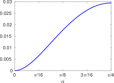
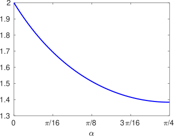
(a) $\frac{(1-p_{x})(1-p_{y})}{p_{x}p_{y}}$	(b) $\frac{p_{x}+p_{y}-p_{x}p_{y}}{p_{x}+p_{y}-1}$

Figure 12: Plots of key quantities used in the proof of Theorem 4.3.

References

- [1] Hamed Ahmadi and Chen-Fu Chiang. Quantum phase estimation with arbitrary constant-precision phase shift operators. Quantum Information & Computation, 12(9&10):0854–0875, 2012.
- [2] Richard Arratia and Louis Gordon. Tutorial on large deviations for the binomial distribution. Bulletin of Mathematical Biology, 51(1):125–131, 1989.
- [3] Alán Aspuru-Guzik, Anthony D. Dutoi, Peter J. Love, and Martin Head-Gordon. Simulated quantum computation of molecular energies. Science, 309(5741):1704–1707, 2005.
- [4] Andrew M. Childs, John Preskill, and Joseph Renes. Quantum information and precision measurement. Journal of Modern Optics, 47(2/3):155–176, 2000.
- [5] Richard Cleve, Arthur Ekert, Chiara Macchiavello, and Michele Mosca. Quantum algorithms revisited. Proceedings of the Royal Society A, 454(1969):339–354, 1998.
- [6] Miroslav Dobšíček, Göran Johansson, Vitaly Shumeiko, and Göran Wendin. Arbitrary accuracy iterative phase estimation algorithm as a two qubit benchmark. Physical Review A, 76(3):030306, 2007.
- [7] Shelby Kimmel, Guang Hao Low, and Theodore J. Yoder. Robust calibration of a universal single-qubit gate set via robust phase estimation. Physical Review A, 92(6):062315, 2015.
- [8] Alexei Yu. Kitaev. Quantum measurements and the Abelian stabilizer problem. arXiv preprint quant-ph/9511026, 1995. (See also Electronic Colloquium on Computational Complexity, TR96-003, 1996).
- [9] Alexei Yu. Kitaev, Alexander H. Shen, and Mikhail N. Vyalyi. Classical and Quantum Computation. American Mathematical Society, 2002.
- [10] Emmanuel Knill, Gerardo Ortiz, and Rolando D. Somma. Optimal quantum measurements of expectation values of observables. Physical Review A, 75(1):012328, 2007.
- [11] Michael A. Nielsen and Isaac L. Chuang. Quantum Computation and Quantum Information. Cambridge University Press, 2010.
- [12] Peter J. J. O’Malley, Ryan Babbush, Ian D. Kivlichan, Jonathan Romero, Jarrod R. McClean, Rami Barends, Julian Kelly, Pedram Roushan, Andrew Tranter, Nan Ding, Brooks Campbell, Yu Chen, Zijun Chen, Ben Chiaro, Andrew Dunsworth, Austin G. Fowler, Evan Jeffrey, Erik Lucero, Anthony Megrant, Josh Y. Mutus, Matthew Neeley, Charles Neill, Chris Quintana, Daniel Sank, Amit Vainsencher, James Wenner, Ted C. White, Peter V. Coveney, Peter J. Love, Hartmut Neven, Alán Aspuru-Guzik, and John M. Martinis. Scalable quantum simulation of molecular energies. Physical Review X, 6(3):031007, 2016.
- [13] Peter W. Shor. Polynomial-time algorithms for prime factorization and discrete logarithms on a quantum computer. SIAM Journal on Computing, 26(5):1484–1509, 1997.
- [14] Krysta M. Svore, Matthew B. Hastings, and Michael Freedman. Faster phase estimation. Quantum Information & Computation, 14(3–4):306–328, March 2014.
- [15] Kristan Temme, Tobias J. Osborne, Karl G. Vollbrecht, David Poulin, and Frank Verstraete. Quantum Metropolis sampling. Nature, 471:87–90, 2011.
- [16] James D. Whitfiled, Jacob Biamonte, and Alán Aspuru-Guzik. Simulation of electronic structure Hamiltonians using quantum computers. Molecular Physics, 109(5):735–750, 2011.
- [17] Nathan Wiebe and Vadym Kliuchnikov. Floating point representations in quantum circuit synthesis. New Journal of Physics, 13:093041, 2013.