Reconstruction of Storage Ring ’s Linear Optics with Bayesian Inference

Abstract

A novel approach of accurately reconstructing the storage ring’s linear optics from turn-by-turn (TbT) data containing measurement error is introduced. This approach adopts the Bayesian Inference process based on the Markov Chain Monte-Carlo (MCMC) method, which is widely used in data-driven discoveries. By assuming a preset accelerator model with unknown parameters, the inference process yields their posterior distribution. This approach is demonstrated by inferring the linear optics Twiss parameters and their measurement uncertainties using a set of data measured at the National Synchrotron Light Source-II (NSLS-II) storage ring. Some critical effects, such as the radiation damping rate, the decoherence due to nonlinearity and chromaticity can also be included in the model and be inferred directly. One advantage of the MCMC based Bayesian inference is that it can be performed with one single set of TbT data to achieve both the inferred results and their uncertainty before a significant machine drift can happen. The precise reconstruction of the parameter in the accelerator model with the uncertainties is crucial prior information to improve machine performance.

I Introduction

In accelerator operations, a significant amount of diagnostic data is recorded to understand the statistical properties of the bunched charge-particles. The diagnostic data may be the first order moment (beam centroid) from beam position monitors (BPMs), second order moment (beam size) or sampling of the beam distribution from the projection on the varies types of the profile monitors. These data are the only clue to tune the control knobs to make the accelerator as the machine we designed.

Among all tuning tasks, the correction of linear optics is one of the most important tasks to improve accelerator performance. A more detailed summary of linear optics measurements has been reviewed in Ref.(Tomás et al., 2017). There are various established methods used to characterize the linear optics experimentally, using the Turn-by-Turn (TbT) BPM data of a storage ring. These include independent component analysis (ICA)(Huang et al., 2005), model-independent analysis (MIA)(Irwin et al., 1999), and orthogonal decomposition analysis (ODA)(Castro-Garcia, 1996) for retrieving the optics functions tunes, dispersions and chromaticities. The decoherence of the beam during the TbT data measurements can be suppressed using pulsed excitation(Malina et al., 2017). Besides the optics measurement, The TbT BPM data is also used in the impedance measurement(Carlà et al., 2016). Another well-developed and widely used method is linear optics from closed orbit (LOCO) (Safranek, 1997), which heavily depends on the lattice model.

In this article, an alternative method is demonstrated to retrieve these machine properties using the Bayesian Inference process from the accelerator diagnostics data. Bayesian Inference is a powerful tool to infer unknown parameters $\theta=\left(\theta_{1},\theta_{2},...,\theta_{N}\right)$ of a preset model from a measurement set $M$. In this method, all to-be-inferred parameters are treated as distribution functions with initial hypothesis $H$, described by its probability $P(H)$. Since the initial hypothesis is assumed before observing any measurement data, it is usually referred to as prior probability. After considering the measurement set $M$, the probability of the hypothesis is modified and becomes the posterior probability $P\left(H\mid M\right)$. Using the Bayes’ theorem, we have

$$P\left(H\mid M\right)=\frac{P\left(M\mid H\right)\cdot P\left(H\right)}{P\left(M\right)}$$ (1)

here, $P\left(M\mid H\right)$ is the probability of the observing $M$ assuming the hypothesis $H$ is valid, also known as the likelihood function. $P\left(M\right)$ is the marginal probability, which does not depend on the hypothesis $H$. Alternatively, $P\left(M\right)$ can be interpreted as the normalization factor calculated from the integral of all possible hypothesis:

$$P\left(M\right)=\int P\left(M\mid H^{\prime}\right)dH^{\prime}.$$ (2)

Directly evaluating the Bayes’ theorem is difficult, not only because of the normalization factor in Eq. 2 usually cannot be integrated explicitly, but also due to the possible high dimension of the unknown parameter space. Therefore, we adopt the memoryless random step search routine, the Markov Chain Monte Carlo (MCMC) methods, to sample the posterior probability which is proportional to

$$P\left(H\mid M\right)\propto P\left(M\mid H\right)\cdot P\left(H\right)$$ (3)

without evaluating $P\left(M\right)$. The detailed algorithm of MCMC is introduced in Appendix A.

We will demonstrate this Bayesian Inference process by determining the linear optics using the BPMs’ TbT data, together with the nonlinear decoherence and the radiation damping effects. The structure of this article is outlined below: we first detail the betatron model and its parameters in the next chapter (chapter II), then illustrate the inference results of the optics function in chapter III, and discuss the model selection criteria for the Bayesian Inference in chapter IV.

The result of the Bayesian Inference, which is the sample from the posterior distribution of the parameter in the model, can play an important role in refining the accelerator settings. In the optics inference example, the posterior distribution of the Twiss parameters will be essential in understanding how well the optics correction can achieve based on the measurement. Recently, a Bayesian approach (Li et al., 2019) was applied for linear optics correction in a storage ring, based on a set of measured linear optics distortions with some uncertainties, and it was noticed that a prior distribution of quadrupole error can be used to specify an optimal regularization coefficient to prevent overfitting.

II Model and Measurement Data

Consider $N$ BPMs distributed around a storage ring. These BPMs can record some selected bunches’ (Li et al., 2017) TbT trajectory for $T$ turns after the beam is excited to perform a betatron oscillation. We can construct a betatron oscillation model to represent the measurement data without detailed knowledge of accelerators, such as the layout of the lattice and the magnet strength. In general the Betatron motion recorded by the $i^{\text{{th}}}$ BPM at $j^{\text{{th}}}$ turn can be written as:

$$x_{i}(j)=x_{c,i}+A_{i}(j)x_{i}(0)\cos\left(2\pi\nu_{x}j+\phi_{i}\right)+\xi_{i}(j)$$ (4)

Here, $x_{c,i}$ is the closed orbit at $i^{\text{{th}}}$ BPM, $\nu_{x}$ is the horizontal betatron tune and $\phi_{i}$ is the phase constant at $i^{\text{{th}}}$ BPM. $A(j)$ is introduced to represent the envelope evolution due to decoherence and radiation damping effect, which will be addressed later. At each turn, the BPM reading contains a random error which follows the Gaussian distribution with a zero mean value and standard deviation $\sigma_{\xi}$.

We treat the first two terms in Eq. 4 as our “model”:

$$x_{i,model}(j)=x_{c,i}+A_{i}(j)x_{i}(0)\cos\left(2\pi\nu_{x}j+\phi_{i}\right)$$ (5)

Then the difference of the measurement data and the model follows a random Gaussian distribution:

$$x_{i,data}-x_{i,model}\propto N(0,\sigma_{xi})$$

for all $j^{\text{th}}$ measurements. The Gaussian random distribution is centered at zero because the bias of the BPM reading and the beam closed orbit $x_{c,i}$ cannot be distinguished by the model in Eq. 5.

The betatron oscillation part of the model can be re-written in terms of the Twiss parameters:

$$\left(\begin{array}[]{c}x_{\beta,i}\\ x_{\beta,i}^{\prime}\end{array}\right)_{j}=A_{i}(j)\left(\begin{array}[]{cc}\cos 2\pi\nu_{x}j+\alpha_{i}\sin 2\pi\nu_{x}&\beta_{i}\sin 2\pi\nu_{x}j\\ \left(-\left(1+\alpha_{i}^{2}\right)\sin 2\pi\nu_{x}j\right)/\beta_{i}&\cos 2\pi\nu_{x}j-\alpha_{i}\sin 2\pi\nu_{x}j\end{array}\right)\left(\begin{array}[]{c}x_{\beta,i}\\ x_{\beta,i}^{\prime}\end{array}\right)_{0}$$

In each turn $j$, the action $J_{i}$ at $i^{\text{th}}$ BPM has the form:

$$J_{i}(j)=\frac{1}{\beta_{i}}\left(x_{\beta,i}^{2}\left(j\right)+\left(\beta_{i}x_{\beta,i}^{\prime}\left(j\right)+\alpha_{i}x_{\beta,i}\left(j\right)\right)^{2}\right)$$

In this form, only information of $x_{\beta}$ can be retrieved from BPM data, while $\beta$, $\alpha$ and $x_{\beta}^{\prime}$ are unknown. We can only infer the combination of these three unknowns. Following the usual accelerator physics notation, we will only infer the conjugate variable pair $\left(x_{\beta},P_{x}\right)$, where the conjugate momentum $P_{x}$ is:

$$P_{x}\equiv\beta x_{\beta}^{\prime}+\alpha x_{\beta}$$

then we can get

$$J_{i}(j)\beta_{i}=x_{\beta,i}^{2}\left(j\right)+P_{x,i}^{2}\left(j\right)$$ (6)

Using the measurement data at each turn, we can infer the betatron oscillation amplitude and the conjugate momentum, hence determine the beta function at each BPM $i$, scaled by the action of the betatron oscillation. In linear optics approximation, the action $J$ is a constant for all BPM locations for any turns after scaled by the envelope factor $A_{i}^{2}(j)$. However, in the experiments at NSLS II, the centroid of the electron beam is kicked to a fraction of 1 mm, thus the nonlinearity of the sextupole cannot be neglected. The simulation shows that the resulting fluctuation of the centroid’s action is a few percent across the BPMs in one turn. We may overcome this difficulty by average the actions over the number of turns of the measurement data. The same simulation shows that the action fluctuation reduces to $6\times 10^{-4}$ after average over 100 turns, and $3\times 10^{-4}$ over 500 turns. Since the accuracy of the beta function usually is expected to be $\sim$1%, we can ignore the fluctuation of the action after averaging it over the measurement time ($\sim$1000 turns).

Finally, a proper form of $A\left(j\right)$ has to be selected to reflect obvious damping behavior. We choose to express the factor inside the exponential function as a polynomial of the turn number:

$$A(j)=\exp\left(-\epsilon_{SR}j-\epsilon_{NL}^{2}j^{2}\right)$$ (7)

Clearly, we can link the coefficients $\epsilon_{SR}$ and $\epsilon_{NL}$ to the synchrotron radiation damping and nonlinear decoherence effect (Meller et al., 1987) respectively. It is worthwhile to note that we took the simplified nonlinear decoherence form (Eq. 18) of reference (Meller et al., 1987). The justification is included in Appendix B.

In this simplified model, we only include the transverse motion in one direction and excluded the effect of chromaticity. The treatment of synchrotron-transverse coupling will be discussed at the end of this article.

Bayesian Inference

The unknown parameters in the model (as in Eq. 5) are noted as $\theta=\left(x_{0,}x_{c},P_{x},\nu_{x},\epsilon_{SR},\epsilon_{NL}\right)$, along with the standard deviation of the Gaussian distribution $\sigma_{\xi}$. These parameters will be inferred from the TbT data $X_{data}=\left(x_{0,}x_{1,}\cdots,x_{T-1}\right)$. Here, the data for each BPM in one measurement is $\sim 2000$ turns. Applying the Bayesian theorem (Eq. 3), we have:

$$P\left(\theta\mid X_{data}\right)\propto P\left(X_{data}\mid\theta\right)P\left(\theta\right)$$

which can be calculated using the MCMC method.

We use a set of measured NSLS-II TbT data to demonstrate this method. The NSLS-II is a 3rd generation light source, which has 30 double bend achromat cells (BNL, ). It is equipped 180 quasi-uniformly distributed BPMs for the purpose of orbit and lattice monitoring and control. The beam can be excited with a horizontal and a vertical fast pulse magnet to perform a free betatron oscillation. The BPMs are configured with TbT resolution and having a gated functionality to lock on a selected diagnostic bunch train (Li et al., 2017). Figure 1 shows one snapshot of TbT data from one of these 180 BPMs.

Figure 1: BPM reading of the first BPM

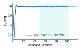
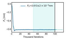
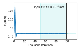
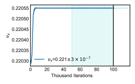
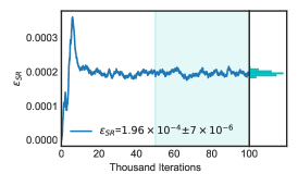
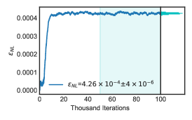
Figure 2: MCMC iterations of parameter $\theta$ using the measurement data of first BPM. From left to right, the top figures are the iterations for $x_{0},$ $P_{x}$ and $x_{c}$; the bottom figures are for $\nu_{x}$, $\epsilon_{SR}$ and $\epsilon_{NL}$ respectively. A histogram plot is attached to the right of the each iteration plot. The histogram is taken from the second half of the total iteration, which is highlighted by the shaded area.

Table 1: Initial values, step sizes and the inference results of parameters in the model Eq.5

	Initial values	Step sizes	Inference results
$x_{0}$ (mm)	$X_{data,0}$	$1\times 10^{-3}$	0.592$\pm 1.4\times 10^{-3}$
$x_{c}$ (mm)	$\bar{X}_{data}$	$1\times 10^{-3}$	0.116$\pm 3.7\times 10^{-4}$
$P_{x}$ (mm)	0	$1\times 10^{-3}$	-0.613$\pm 1.5\times 10^{-3}$
$\nu_{x}$	Peak of DFT	$1\times 10^{-7}$	0.22055$\pm 2.7\times 10^{-7}$
$\epsilon_{SR}$	0	$1\times 10^{-6}$	$1.96\times 10^{-4}$$\pm 7\times 10^{-6}$
$\epsilon_{NL}$	0	$1\times 10^{-6}$	$4.26\times 10^{-4}$$\pm 4\times 10^{-6}$
$\delta_{\xi}$ (mm)	$1\times 10^{-3}$	$1\times 10^{-3}$	0.0164$\pm 2.7\times 10^{-4}$

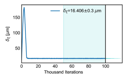
Figure 3: MCMC iteration of the width of the Gaussian error.

The BPM reading reflects the orbit excursion, due to closed orbit, initial beam kick, the machine properties, and the TbT reading errors. The BPM random error of one turn is independent of the measurement of other turns and assumed to be Gaussian random distribution. Therefore the likelihood $P\left(X_{data}\mid\theta\right)$ can be expressed as:

$$P\left(X_{data}\mid\theta\right)\propto\exp\left(-\frac{1}{2\sigma_{\xi}^{2}}\sum_{j=0}^{T-1}\left(x_{data,j}-x_{model,j}\right)^{2}\right)$$

The prior probability $P\left(\theta\right)$ reflects our foreknowledge of these parameters before the measurement. For example, it is expected that the parameter $x_{0}$ should be very close to the first value of measurement data $x_{data,0}$; the closed orbit parameter should be close to the average value of the measurement $\bar{X}_{data}$, while the transverse tune $v_{x}$ is expected to be close to the discrete Fourier transform (DFT) of the BPM data. In addition, the prior distribution can also be used to confine the range of the parameter, such as confining the parameter $\epsilon_{SR}$ and $\epsilon_{NL}$ to be positive. A proper prior will improve the MCMC convergence efficiency and conversely, while incorrect prior will bias the posterior distribution.

In this model, we do not imply any specific prior distribution other than requiring $\epsilon_{SR}$ and $\epsilon_{NL}$ to be positive. The initial value and the step size of each parameter are given in Table 1. The initial value of each parameter reflects the ’best-guess’ value for the corresponding parameter. The choice of step size also plays an important role in the inference process. A small step size would require long iteration steps and long computation time, while a large step size will result in failing to reach convergence. A proper choice of the step size of one parameter should be smaller than the order of the uncertainty of the parameter. In this example, the step sizes of $x_{0}$, $x_{c}$,$P_{x}$ $\delta_{\xi}$ are set to 1 micron, based on a reasonable guess that the NSLS-II BPMs have TbT resolution around 10 microns. The proper step sizes of other parameters are determined by various trials with simulations.

Figure 2 and Figure 3 show the MCMC iterations for the data from one of the BPM. All figures illustrate convergence results after 25000 iterations. The parameter values of each iteration after convergence reaches (cyan shaded area in each figure) can be used to calculate the posterior distribution. The histogram can be plotted to represent the distribution and is attached to the right of each iteration plot. The converged results and their standard deviations are listed in the last column of Table 1.

It is important to note that the uncertainties are obtained from one snapshot of data ($\sim 2000$ turns) using the Bayesian inference. Comparing with other methods, such as ICA, MIA, and ODA, each snapshot can give one measurement result and the uncertainty is obtained from repetitive measurements. However, the machine has been observed continuously drifting during repetitive data collection. Therefore the uncertainty from repetitive measurement is over-estimated with the traditional methods. The overestimated uncertainty could potentially affect the ultimate performance of linear optics correction (Li et al., 2019).

A notable feature of the inferred tune can be found in the bottom left plot of Figure 2 and the inference results in Table 1. The initial guess of the transverse tune from the peak DFT position of the BPM’s data is not precise enough due to a limited length of the data. The inferred tune has much higher accuracy ($\sim 10^{-7}$ compared with $\sim 1/T$, $T$ is the number of turns). The high accuracy of the inferred tune using Bayesian Inference is because of fitting the data with the given model, which is similar to the numerical analysis of fundamental frequency (NAFF) (Laskar et al., 1992) method. The NAFF method aims at precisely searching for a series of orthogonal frequencies using one snapshot of the measurement data. The uncertainty can be retrieved from multiple measurements (Langner and Tomás, 2015; Biancacci and Tomás, 2016; Persson et al., 2017). With the MCMC algorithm, Bayesian Inference achieves not only a precise tune but a sound quantification of the uncertainty with one single snapshot. In addition to the pure betatron oscillation, it is convenient to achieve additional envelop profiles according to the physics knowledges, which is represented by the envelope factor $A\left(j\right)$ in our model. It is worthwhile to note that many forms of envelope function will change the frequency of the oscillation, although the change may be small enough to neglect in real applications.

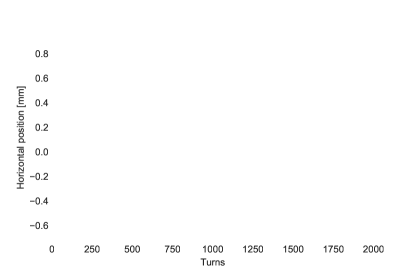
Figure 4: Reconstruction of the first BPM reading using model with inferred parameter (blue) and the difference with the measurement data (orange)

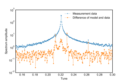
Figure 5: The frequency spectrum of measurement data of the BPM (blue points) and the difference between measurement and model with inferred parameters (orange points)

Figure 4 shows that the model with the inferred parameter represents the measurement data plausibly, with the difference plotted in orange dots. The difference is assumed as a Gaussian random number and is characterized by its standard deviation $\sigma_{\xi}$. However, our model in Eq. 5 cannot reflect all physics in the accelerator completely. The difference in the measurement data and the model prediction must contain other signals rather than pure BPM noises. Therefore, the estimation of $\sigma_{\xi}$ only gives an upper bound on the actual BPM noises. Fourier analysis gives the frequency content of the difference data as shown in figure 5. Clearly, the transverse coupling signal at a tune of about 0.26 is observed, as well as two synchrotron sidebands, about 0.009 away from the transverse tune 0.222.

As pointed out in the previous section, the initial position $x_{0}$, and its conjugate momentum $P_{x,0}$ can be inferred from the data. Then, as shown in Eq. 6, the product of the beta function and the action can be determined for this BPM:

$$\beta J =\left(x_{0}-x_{c}\right)^{2}+P_{x}^{2}$$

$$=0.602\pm 0.003\text{mm}^{2}$$

The inference process is repeated and get the $\beta J$ for all BPMs. The action of the centroid can be averaged over the measurement period. The fluctuation of the average value is less than $4\times 10^{-4}$ for all BPMs, according to the particle simulation using the NSLS-II lattice model. The action is almost constant when compared with the uncertainty of the $\beta J$. However, we can not retrieve the value of $J$ from the BPM data. We have to choose a constant $J$ so that the average of the inverse beta function $\overline{1/\beta}$ equals that calculated from the accelerator model. This step of scaling only aims at producing inferred beta function in the familiar range. Figure 6 shows the inferred beta functions and its error bars, which is barely visible in this plotting scale. For better visibility, only beta functions at the first 90 BPMs are plotted. The average standard deviation of beta functions is about 0.47%, while the difference of beta function from the model and the measurement is 10% peak to peak, as shown in the green dots of Figure 6. Therefore there is a large potential for the optics to be corrected. In the optics correction process, the uncertainty of the optics function and phase advance, retrieved from the Bayesian Inference, can be used directly to define the regularization coefficients in order to prevent overfitting issue, as pointed out in (Li et al., 2019).

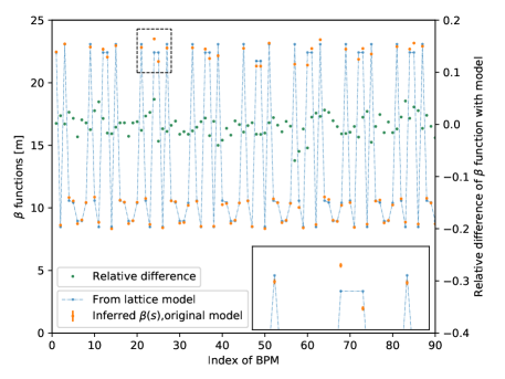
Figure 6: The inferred beta function at first 90 BPMs and its standard deviation error (orange dots), with the beta function calculated from bare lattice (in blue doted lines) as a reference. The relative difference of the inferred beta function and the model is shown in green dots.

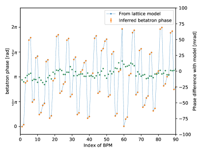
Figure 7: The inferred betatron phase at first 90 BPMs (orange dots), with the betatron phase advance calculated from bare lattice (blue doted line) as reference. The phase difference is shown in the green dots.

The betatron phase $\phi_{\beta}$ is calculated as:

$$\phi_{\beta}=\arctan\left(\frac{P_{x}}{x_{0}-x_{c}}\right)$$

Figure 7 compares the inferred betatron phase and the phase calculated from the accelerator model. The standard deviations of the betatron phase vary from $1.5\times 10^{-3}$ and $3\times 10^{-3}$ rad, therefore they are not visible in the figure.

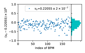
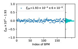
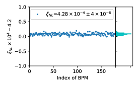
Figure 8: The tune, $\epsilon_{SR}$ and $\epsilon_{NL}$ inferred from all 180 BPMs. For easier reading, they are rescaled and shifted to the range [-1,1]. The quantity bing plotted are left: $\left(\nu_{x}-0.22055\right)\times 10^{6}$, middle: $\epsilon_{SR}\times 10^{4}-1.93$ and right: $\epsilon_{NL}\times 10^{4}-4.20$.

Table 2: Comparison of standard deviation of the mean values of 180 inferences and the average of the standard deviation in each inference.

	Standard deviation of mean value of 180 inferences	Average of the uncertainty of each mean value
$\nu_{x}$	$1.9\times 10^{-7}$	$3.4\times 10^{-7}$
$\epsilon_{SR}$	$5.5\times 10^{-6}$	$6.0\times 10^{-6}$
$\epsilon_{NL}$	$3.6\times 10^{-6}$	$4.1\times 10^{-6}$

We expect a priori that the parameter $\nu_{x}$, $\epsilon_{SR}$, and $\epsilon_{NL}$ should be common to the entire ring, as they are the ’integrating’ parameters and reflects the dynamics of the entire ring. Thus it is a useful step to check that the inference produces consistent values across all BPMS. Figure 8 shows the inferred mean values of $\nu_{x}$, $\epsilon_{SR}$, and $\epsilon_{NL}$ from data of 180 BPMs, and their histograms are attached to the right. Table 2 illustrates that the deviation of the mean values of the 180 inference results is less than the average of the uncertainty (standard deviation) of each mean value. It supports our belief that we can infer very similar values of $\nu_{x}$, $\epsilon_{SR}$, and $\epsilon_{NL}$ from all BPMs, as it should be from the physics behind the model.

Model Selection

The results in the previous sections are based on the assumed model in Eq. 5. A valid model is key to the success of Bayesian inference. The model itself can be also viewed as the strongest prior information, which enhances a finer treatment than considering the accelerator as a black box. The confidence of placing these models based on physics knowledge, instead of other general models such as an artificial neural network, relies on the belief that the accelerator model can represent most of the physics in an accelerator. In this chapter, we discuss the strategy of model selection in Bayesian Inference.

One could choose a very precise model with detailed accelerator elements such as the magnets, cavities and the drift space between them. The currents, voltage and the geometric information (length, distances) will be the unknown parameters to be inferred from measurement data. However, it is impractical, at least for the computation power nowadays, to infer such a high-dimensional problem, as there are usually thousands of knobs to describe accelerator lattice to be inferred, even with strong prior assumptions and a large amount of data. Meanwhile, in most cases, the goal of optimizing accelerator operation is not to know every detail of accelerators, but the key parameters that affect the performance, for instance, the beam behavior at the interaction point in colliders or at the insertion devices of synchrotron light sources.

Therefore it is reasonable to choose the model to represent the dynamics of interest with few parameters. In our example the previous chapter, the focus is only on betatron motion and its damping envelope, as in Eq. 5. In many existing methods, the damping envelope is ignored, which corresponds to adjust our model by forcing $A\left(j\right)\equiv 1$. This reduces the model to

$$x_{i,model}(j)=x_{c,i}+x_{i}(0)\cos\left(2\pi\nu_{x}j+\phi_{i}\right)$$ (8)

where only four parameters $\theta_{reduced}=\left(x_{0,}x_{c},P_{x},\nu_{x}\right)$ will be inferred. We refer to this model as a “reduced model” from now on. Using less number of parameters decreases the iterations required to reach equilibrium, as well as the computation time.

From the reduced model, the betatron tune is systematic higher than that from the original model, due to the term $A(j)$ in the original model shifts the sinusoidal frequency. The average tune difference of all BPMs is as small as the $1.7\times 10^{-6}$, which is sufficiently small for almost any real application. inferred optics and its uncertainty between the two models. What distinguishes the reduced model and the original model, is the confidence of the inferred optics functions.

Figure 9 shows the comparison of the inferred beta function of the reduced model and the original model. With the reduced model (Eq. 8) we have overlapped the mean value of the beta function from the mean values of the original model, with about a 0.4% standard deviation. However, the uncertainty of the beta function on average increases by about 4.4 times compared with the original model. The betatron phase advance of the reduced model also has larger uncertainties, ranging from 0.01 to 0.015 rad. They are about 5 times larger than that of the original model. The uncertainty of the optics function may play an important role in the lattice correction as pointed out in Ref (Li et al., 2019).

It is worthwhile to note that the “reduced model” is not an incorrect model. The results from the reduce model just have larger uncertainties. They can be used as the prior distribution if we extend the model to include the decoherence effect as in Eq. 5.

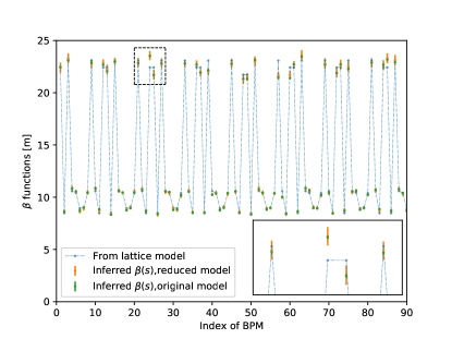
Figure 9: The inferred beta function at first 90 BPMs with the original and reduced model.

For the factor $A(j)$, it is also worthwhile to note that the choice of the quadrature form $\exp\left(-\epsilon_{SR}j-\epsilon_{NL}^{2}j^{2}\right)$ is not arbitrary. On the one hand, we understand that these two terms have their physics meaning. On the other hand, we may also get hint only from the BPM data pretending to have no accelerator physics knowledge on nonlinear decoherence. If $A(j)$ only has the form of the exponential decay term:

$$A(j)=A(0)\exp\left(-\epsilon_{SR}j\right)$$

where $A(0)=1$. The envelope decay would be “memoryless”, viz. we expect the same parameter $\epsilon_{SR}$, no matter from which turns we start our analysis. If we start our analysis from $m^{\text{th}}$ turn:

$$A(j+m) =A(0)\exp\left(-\epsilon_{SR}\left(j+m\right)\right)$$

$$=A(0)\exp\left(-\epsilon_{SR}m\right)\exp\left(-\epsilon_{SR}j\right)$$

$$=A(m)\exp\left(-\epsilon_{SR}j\right)$$

We can test by selecting 1000-turn data out of the total 2000 turns with varying starting turns and used to infer the model which contains $A(j)=\exp\left(-\epsilon_{SR}j\right)$ and found that the inferred $\epsilon_{SR}$ is not a constant, as shown in Figure 10.

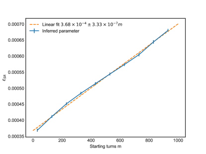
Figure 10: The inferred $\epsilon_{SR}$ from 1000 turns data with varying starting turns.

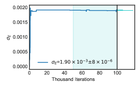
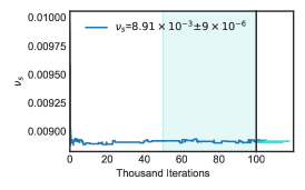
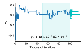
Figure 11: The inference of the synchrotron oscillation parameters Left: $\epsilon_{E}=\xi\sigma_{E}$, middle: $\nu_{s}$ right: synchrotron phase $\phi_{s}$.

Instead of a flat dependence on the starting turn $m$, the inferred $\epsilon_{SR}$ is approximately a linear function of $m$ with a significant slope. Therefore it suggests that the model is not “memoryless” and can not be modeled simply by an exponential decay function. We may improve the model by adding an unknown function $f(j)$:

$$A(j)=A(0)\exp\left(-\epsilon_{SR}j-f(j)\right)$$ (9)

If we start inference at turn $m$, factor $A(j)$ should reads:

$$A(j+m)=A(0)\exp\left(-\epsilon_{SR}\left(j+m\right)-f(j+m)\right)$$ (10)

Meanwhile, if the slope in Figure 10 denoted as $\kappa$, the exponential decay rate starting at turn $m$ is approximately $\epsilon_{SR}(m)=\epsilon_{SR}+\kappa m$. $A(j+m)$ can be rewritten as:

$$A(j+m) =A(m)\exp\left(-\left(\epsilon_{SR}+\kappa m\right)j-f(j)\right)$$

$$=A(0)\exp\left(-\left(\epsilon_{SR}+\kappa m\right)j-\epsilon_{SR}m-f(m)-f(j)\right)$$

$$=A(0)\exp\left(-\epsilon_{SR}\left(j+m\right)-f(m)-f(j)-\kappa mj\right)$$ (11)

From Eq. 10 and 11, the extra term $f$ should satisfy:

$$f(j+m)=f(j)+f(m)+\kappa mj$$ (12)

in order to represent the linear slope in Figure 10. The simplest form of function $f$ is the quadrature form $f(j)\propto j^{2}$. Therefore, learning from the data, we confirm that the simplified model of decoherence factor $A\left(j\right)$ in Eq.7 is a reasonable and simple choice.

Our model (as in Eq.5) certainly will not reflect all physics hidden in the data. Figure 5 indicates that there are still signals in the difference between the data and the model. It is easy to identify the synchrotron sidebands and the transverse coupling as stated in the previous sections. If this information is needed, a more precise model can be adopted. For instance, we can extend the model to extract the chromatic decoherence, by modifying the decoherence term $A(j)$ as:

$$A\left(j\right)=\exp\left(-\epsilon_{SR}j-\epsilon_{NL}^{2}j^{2}-\frac{\alpha^{2}(j)-\alpha^{2}(0)}{2}\right)$$

with the new function $\alpha(j)$ has the form:

$$\alpha(j)=\frac{2\xi_{x}\sigma_{E}}{\nu_{s}}\sin\left(\pi\nu_{s}j+\phi_{s}\right)$$

which is representing the chromaticity decoherence (Meller et al., 1987). $\xi_{x}$ is the linear chromaticity of $x$-direction, $\sigma_{E}$ is the RMS energy spread, $\nu_{s}$ is the synchrotron tune and $\phi_{s}$ is the synchrotron phase. Using this synchro-betatron model, three more parameters can be extracted, which are $\epsilon_{E}=\xi_{x}\sigma_{E}$, $\nu_{s}$ and $\phi_{s}$, in additional to the parameters $\theta=\left(x_{0,}x_{c},P_{x},\nu_{x},\epsilon_{SR},\epsilon_{NL}\right)$ in the original model. Based on the fact that the synchro-betatron mode is a small perturbation of the betatron motion, the mean values of the inference results from the original model can be used as the prior information to infer the synchro-betatron parameters. Figure 11 demonstrates the inference results of the 9${}^{\text{th }}$ BPM. The product $\xi_{x}\delta_{E}$ saturates at $1.9\times 10^{-3}$ with standard deviation of $8\times 10^{-6}$. This is consistent with the estimated chromaticity $\sim 2$ and RMS energy spread of $\sim 9\times 10^{-4}$. The inferred synchrotron tune also meets the values from the lattice model. The minimization of the model and the data is a weaker function of the synchrotron phase, therefore the synchrotron phase has a large standard deviation from its inferred value.

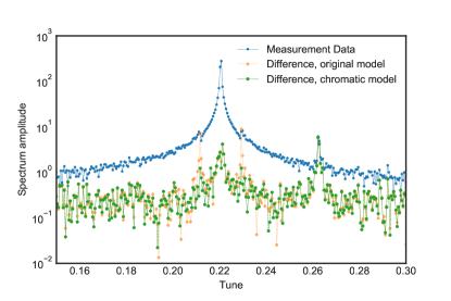
Figure 12: Frequency spectrum of the measurement data (blue dots) and residue between measurement and model with inferred parameters of the 9${}^{\text{th }}$ BPM, using the original model (orange dots) and the model with chromatic decoherence (green dots)

Figure 12 demonstrates that after using the chromatic decoherence term in $A(j)$, we can eliminate the two synchrotron sideband from the frequency spectrum of the difference of the measurement and the model.

However, the convergence of inferring chromatic decoherence varies among all BPMs. For some BPMs, very long iterations (larger than 200 thousand iterations) is needed, inferred synchrotron tuning from some BPM may yield twice of the synchrotron tunes. This issue is likely related to the fact that the chromatic decoherence is a much weaker signal compared with the betatron motions. Actually, it is not wise to extract very small signal using the Bayesian Inference. If the synchrotron motion is of interest, we should design another experiment with perturbed longitudinal motions and infer the unknowns with the corresponding models. The statistics property obtained from this article can be used as prior information of the transverse optics in the next inference process. The Bayes’s theorem enables us to sequentially update our understanding of an accelerator by serials of measurements and the evolution of the models. We will demonstrate this benefit in future works.

Summary

In this paper, we introduce a new approach to infer the parameters of the accelerator model, using the measured TbT data in MCMC algorithm based Bayesian Inference. It requires our prior knowledge, which includes a proper accelerator model with parameters to be determined and our belief (prior distribution) on the parameters. The MCMC algorithm used in Bayesian Inference can generate samples from the posterior distribution of the unknown parameters in the model using only a single snapshot of measurement data. From the samples, the most probable values of the parameters and their standard deviation are obtained. Using the Bayesian approach, multiple data requisition is not necessary. Therefore, pollution due to the slow drift of machine parameters and the environment is mitigated or significantly reduced. In addition, the model used in the inference can be easily extended or refined, either from the accelerator physics knowledge or from the data analysis. If a model needs to be extended from its original form, the posterior distribution of the original model can serve as the prior distribution of the extended one.

A proof-of-concept example has been demonstrated by exploring the inference of optics functions of the betatron motion in the horizontal plane, using measurement data of the NSLS-II electron storage ring. There is no foreseen difficulty to apply the method to hadron rings. A direct application of the reconstructed optics functions is the optics correction. As pointed out in Ref (Li et al., 2019), the statistical properties of the optics function will gain more insight into the optics correction process by avoiding over-fitting. This approach could also be potentially extended to analyzing more complicated dynamics in accelerators, such as determining coupling coefficient, analyzing the nonlinear dynamics properties, or estimate the reliability of each instrumentation devices.

Appendix A: Markov Chain Monte-Carlo Method

Markov Chain Monte-Carlo (MCMC) is a powerful method, which can sample the posterior distribution of the parameters of interest. It is especially useful when in Bayesian Inference case (Eq.1), since the marginal distribution $P\left(M\right)$ is usually impossible to be directly calculated. The MCMC method constructs a Markov chain, whose equilibrium distribution is proportional to the product of the likelihood and prior distribution, and sample it using Monte-Carlo method. The details of MCMC can be found in many text books, such as Chapter 10 in Ref (Ross, 2006). Here we only outline the MCMC algorithm used this article.

We use the Hastings-Metropolis algorithm, an MCMC algorithm, to get the sample of random variable $\theta^{i}$, with $i$ as the iteration index, whose limiting probability is the posterior distribution $P\left(\theta\mid M\right)$. The algorithm is detailed as below procedures:

1. Choose initial condition ($0^{\text{th}}$ iteration) $\theta^{0}$. The choice does not affect the inference result. However, a reasonable guess of the initial condition reduces the required iteration to reach equilibrium.

2. Evaluate the $\pi(i)=P\left(M\mid\theta^{i}\right)\cdot P\left(\theta^{i}\right)$ for the $i^{\text{th}}$ iteration

3. Make Gaussian random walk centered at the value of $\theta^{i}$, with preset step size as the standard deviation, to get the new trial parameters $\theta^{t}$

4. Evaluate the $\pi(t)=P\left(M\mid\theta^{t}\right)\cdot P\left(\theta^{t}\right)$

5. Get a sample $u$ from uniform random distribution $[0,1]$

6. If $u<\min\left(\frac{\pi\left(t\right)}{\pi\left(i\right)},1\right)$, the random walk is accepted, $\theta^{i+1}=\theta^{t}$; otherwise $\theta^{i+1}=\theta^{i}$

We continue this procedure for $N$ iterations. If after first $n\left(<N\right)$ iterations, the chain reaches its equilibrium, then the sequence $\left(\theta^{n+1},\theta^{n+2},\cdots,\theta^{N}\right)$ is the desired sampling of the posterior distribution of $\theta$.

Appendix B: Model for Nonlinear Decoherence

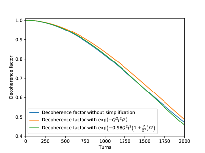
Figure 13: The comparison of different decoherence model.

In Ref (Meller et al., 1987), the decoherence factor of the beam centroid motion due to nonlinearity is given by Eq. 20, which can be written using the notation in this article:

$$A(j)=\frac{1}{1+Q^{2}j^{2}/Z^{2}}\exp\left[-\frac{Q^{2}j^{2}/2}{1+Q^{2}j^{2}/Z^{2}}\right]$$ (13)

where $Z=\beta\Delta x^{\prime}/\sigma_{x}$ denotes the the normalized strength of the kick angle, $Q=-4\pi Z\nicefrac{{d\nu}}{{da^{2}}}$ represents the effect of detuning and $a=\sqrt{\beta\epsilon}/\sigma_{x}$ is the betatron amplitude scaled by rms beam size.

The Gaussian decoherence approximation is given by the Eq. 18,

$$A(j)\approx\exp\left[-\frac{Q^{2}j^{2}}{2}\right]$$ (14)

if the amplitude tune dependence is small and the observation time is short. The condition for a such approximation is

$$Z\gg QN\text{ or }4\pi\left|\frac{d\nu}{da^{2}}\right|N\ll 1$$ (15)

for $N$-turns data set.

The gaussian form of the decoherence factor is preferred in the Bayesian inference since the only one parameter $Q$ is used, while in the general form (Eq. 13), an additional parameter $Z$ is needed.

In the NSLS-II example, the transverse kick strength $Z$, which excites the betatron oscillation, is about 3.7. The NSLS-II model predict that the amplitude tune dependence $\nicefrac{{d\nu}}{{da^{2}}}$ is $-1.28\times 10^{-5}$ by assuming the horizontal emittance as $2.1\times 10^{-9}$ nm rad, hence $QN/Z$ equals 0.32 for 2000 turns data, which is not much less than 1. Therefore, the condition (Eq. 15) is not fully satisfied. The difference between two forms (Eq. 13 and 14) is shown from the blue and orange lines in Figure13.Since the difference is small over the 2000 turns, we are motivated to seek for an alternated Gaussian form by modifying the exponential term.

Slightly modifying Eq. 14, we use the following Gaussian form

$$A(j)\approx\exp\left[-\frac{rQ^{2}j^{2}}{2}(1+\frac{2}{Z^{2}})\right]$$ (16)

which deviates from the general decoherence form (Eq. 13) by $\mathcal{O\text{$\left(Q^{4}j^{4}\right)$}}$ when the factor $r=1$. The green line in Figure13 shows that by adjusting the factor $r$, eg. $r=0.98$ in the plot, we can achieve approximate the general decoherence factor within the length of dataset.

References

- Tomás et al. (2017) R. Tomás, M. Aiba, A. Franchi, and U. Iriso, Phys. Rev. Accel. Beams 20, 054801 (2017).
- Huang et al. (2005) X. Huang, S. Y. Lee, E. Prebys, and R. Tomlin, Phys. Rev. ST Accel. Beams 8, 064001 (2005).
- Irwin et al. (1999) J. Irwin, C. X. Wang, Y. T. Yan, K. L. F. Bane, Y. Cai, F.-J. Decker, M. G. Minty, G. V. Stupakov, and F. Zimmermann, Phys. Rev. Lett. 82, 1684 (1999).
- Castro-Garcia (1996) P. Castro-Garcia, Luminosity and beta function measurement at the electron - positron collider ring LEP, Ph.D. thesis, CERN (1996).
- Malina et al. (2017) L. Malina, J. Coello de Portugal, T. Persson, P. K. Skowroński, R. Tomás, A. Franchi, and S. Liuzzo, Phys. Rev. Accel. Beams 20, 082802 (2017).
- Carlà et al. (2016) M. Carlà, G. Benedetti, T. Günzel, U. Iriso, and Z. Martí, Phys. Rev. Accel. Beams 19, 121002 (2016).
- Safranek (1997) J. Safranek, Nuclear Instruments and Methods in Physics Research Section A: Accelerators, Spectrometers, Detectors and Associated Equipment 388, 27 (1997).
- Li et al. (2019) Y. Li, R. Rainer, and W. Cheng, Phys. Rev. Accel. Beams 22, 012804 (2019).
- Li et al. (2017) Y. Li, W. Cheng, K. Ha, and R. Rainer, Phys. Rev. Accel. Beams 20, 112802 (2017).
- Meller et al. (1987) R. E. Meller, A. W. Chao, J. M. Peterson, S. G. Peggs, and M. Furman, SSC-N-360 (1987).
- (11) BNL, https://www.bnl.gov/nsls2/project/PDR/.
- Laskar et al. (1992) J. Laskar, C. Froeschlé, and A. Celletti, Physica D: Nonlinear Phenomena 56, 253 (1992).
- Langner and Tomás (2015) A. Langner and R. Tomás, Phys. Rev. ST Accel. Beams 18, 031002 (2015).
- Biancacci and Tomás (2016) N. Biancacci and R. Tomás, Phys. Rev. Accel. Beams 19, 054001 (2016).
- Persson et al. (2017) T. Persson, F. Carlier, J. C. de Portugal, A. G.-T. Valdivieso, A. Langner, E. H. Maclean, L. Malina, P. Skowronski, B. Salvant, R. Tomás, and A. C. G. Bonilla, Phys. Rev. Accel. Beams 20, 061002 (2017).
- Ross (2006) S. M. Ross, Simulation (4.th ed.) (Elsevier, 2006).