Toward computing sensitivities of average quantities in turbulent flows

Chaotic dynamical systems such as turbulent flows are characterized by an exponential divergence of infinitesimal perturbations to initial conditions. Therefore, conventional adjoint/tangent sensitivity analysis methods that are successful with RANS simulations fail in the case of chaotic LES/DNS. In this work, we discuss the limitations of current approaches, including ensemble-based and shadowing-based sensitivity methods, that were proposed as alternatives to conventional sensitivity analysis. We propose a new alternative, called the space-split sensitivity (S3) algorithm, that is computationally efficient and addresses these limitations. In this work, the derivation of the S3 algorithm is presented in the special case where the system converges to a stationary distribution that can be expressed with a probability density function everywhere in phase-space. Numerical examples of low-dimensional chaotic maps are discussed where S3 computation shows good agreement with finite-difference results, indicating potential for the development of the method in more generality.

 

1 Introduction

Conventional tangent/adjoint sensitivity analysis methods have been extensively applied to RANS simulations for uncertainty quantification, mesh adaptation and gradient-based multidisciplinary design optimization applications (Blonigan, 2017; Samareh, 2001). Many modern applications require computing sensitivities in DNS/LES; examples include buffet prediction in high-maneuverability aircraft, modern turbomachinery design and jet engine and airframe noise control. The methodologies for sensitivity analysis in these high-fidelity simulations must be more sophisticated than the conventional tangent/adjoint approaches since the latter are known to produce meaningless sensitivities of statistically stationary quantities under chaotic dynamics (Ni & Wang, 2017; Wang, 2014).

In the next section, we discuss the deficiencies of current alternative methods, including ensemble-based and shadowing-based methods. In particular, ensemble-based methods are prohibitively expensive owing to the inherent instability and associated high uncertainty of tangent, adjoint and finite-difference methods in chaotic systems. Shadowing-based methods do not always compute the correct sensitivities since they are based on determining stable, shadowing perturbations that are not guaranteed to carry the correct average information about the flow. The purpose of this work is to develop a new methodology, called the space-split sensitivity (S3) algorithm, that addresses these deficiencies to produce a provably convergent and computationally efficient means to compute sensitivities of statistical averages to input parameters.

The strategy used by S3 to circumvent the ill-conditioning of tangent and adjoint equations deviates from that of both ensemble-based and shadowing-based approaches. While ensemble sensitivity suffers because of the unbounded variance of the unstable contribution to the overall sensitivity, S3 splits the contributions and performs a finite-sample averaging only in order to obtain the stable contribution. The unstable contribution is manipulated through integration-by-parts and with ergodic properties of the fluid flow to yield an algorithm that does not use unstable tangent solutions. Since both parts of the sensitivity are computed through sampling on generic flow trajectories, the problem of the computed sensitivities corresponding to unrepresentative trajectories, which shadowing-based methods are vulnerable to, is averted. In Section 3, we elucidate these key ideas of stable-unstable splitting and of the modification of the unstable contribution. We describe the algorithm derived under simplifying mathematical assumptions in Section 4 and demonstrate the algorithm on low-dimensional numerical examples in Section 5.

2 Current methods and their limitations

Consider a chaotic map parameterized by a set of parameters $s$,

$$u_{i+1}=\varphi^{s}(u_{i}),\>i=0,1,2\cdots,u_{i}\in\mathbb{R}^{n}.$$ (1)

In a fluid simulation, the state vector $u_{i}$ consists of all the unknowns at the timestep $i$, such as the density, velocity components and pressure at all the grid points, and in this case, $n=5\times$ the number of grid points. The transformation $\varphi^{s}$ is the Navier-Stokes solver that advances the state by one timestep, with examples of $s$ being geometric parameters of the domain or inlet conditions and so on. The fluid state $u_{i}$ can be written as a function of the initial state $u_{0}$ as $u_{i}=\varphi^{s}_{i}(u_{0})$, where the subscript $i$ in $\varphi_{i}^{s}$ refers to solving for $i$ timesteps; that is, $\varphi_{i}^{s}=\underbrace{\varphi^{s}\circ\cdots\circ\varphi^{s}}_{i\;{\rm times}}$. We also use the notation $\varphi_{-i}^{s}$ to denote the transformation $(\varphi^{s})^{-1}$ composed with itself $i$ times to indicate solving backward in time by $i$ timesteps; that is, $\varphi_{-i}(u_{i})=u_{0}$.

We are concerned with statistically stationary fluid systems where the state vector has achieved a stationary probability distribution $\mu^{s}$ in phase-space. The superscript $s$ in $\mu^{s}$ indicates that the distribution depends on the input parameters. We are interested in determining the sensitivity of the statistical average, with respect to the distribution $\mu^{s}$, of a scalar objective function $J$ denoted by $\langle J\rangle:=\int J\;d\mu^{s}$, to $s$. Examples of objective functions include lift and drag over wings and pressure losses in turbine wakes. Under the assumption of ergodicity, the statistical average of a bounded function $J$ is also observed as an infinite time average along almost every flow trajectory. That is, if $J\circ\varphi_{i}^{s}(u_{0})$ is the instantaneous value of $J$ at timestep $i$ starting at $u_{0}$, then $\lim_{N\to\infty}(1/N)\sum_{i=0}^{N-1}J\circ\varphi_{i}^{s}(u_{0})=\langle J\rangle$ for almost every initial condition $u_{0}$. This infinite time average, called the ergodic average, is the more natural form of $\langle J\rangle$ from the simulation standpoint, since it can be obtained by measurements of $J$ along trajectories. The ergodic average up to a large $N$ is used in practice to approximate the ensemble average $\langle J\rangle$.

2.1 Ill-conditioned conventional tangent and adjoint methods

When the notation $v_{i}(u_{0}):=(d\varphi_{i}^{s}/ds)(u_{0})$ is used, the familiar tangent equation derived by means of a linear approximation of the transformation $\varphi_{i}^{s}$ around the reference value of $s$ is given by,

$$v_{i+1}(u_{0}) =D\varphi^{s}(u_{i})v_{i}(u_{0})+\frac{\partial\varphi^{s}}{\partial s}(u_{i}),\;i=0,1,\cdots$$

$$v_{0}(u_{0}) =\frac{du_{0}}{ds}=0\in\mathbb{R}^{n},$$ (2)

where $(D\varphi^{s})(u_{i})$ is the Jacobian matrix evaluated at $u_{i}$ [$Df$ denotes differentiation of a function $f$ with respect to a phase point and $(Df)(u)$ refers to the value of the derivative at the point $u$]. In a conventional tangent sensitivity computation, we simply apply the chain rule to calculate the instantaneous sensitivity of the scalar field $J\circ\varphi_{i}^{s}$ as $d_{s}(J\circ\varphi_{i}^{s})=(DJ)(u_{i})\>v_{i}$. In any chaotic system, $\lVert v_{i}(u_{0})\rVert\sim{\cal O}(\exp(\lambda i)),$ $\lambda>0$ (the largest among the so-called Lyapunov exponents), for almost every $u_{0}$; therefore, the instantaneous sensitivity $d_{s}(J\circ\varphi_{i}^{s})$ also grows in norm exponentially with $i$. Since $\langle J\rangle$ is equal to its infinite time ergodic average, one may naturally try to compute $d_{s}\langle J\rangle$ by using the instantaneous sensitivities obtained with the tangent vectors as $\lim_{N\to\infty}(1/N)\sum_{i=0}^{N-1}(DJ)(u_{i})\>v_{i}$. But the latter quantity is unbounded, whereas the correct sensitivity is a finite quantity, thereby rendering the sensitivities computed from the tangent equation meaningless for large $i$. Since the adjoint equation when solved backward in time also has exponentially diverging solutions, sensitivities computed by using the adjoint method are also unbounded for large $i$.

2.2 Ensemble sensitivity analysis and its computational expense

The Lea-Allen-Haine ensemble sensitivity method (Eyink et al., 2004) suggests a simple work-around to the exponentially diverging sensitivities computed by the conventional tangent/adjoint methods. The work-around is to truncate the values of $i$ at a finite $N$ that represents an intermediate timescale on the same order as $1/\lambda$ and instead introduce phase-space averaging over a finite sample of independent trajectories. The rigorous justification for this approximation is given by a statistical response formula due to Ruelle (1997), which describes the sensitivity we want to compute as a summation, where each summand is a phase-space average

$$\frac{d\langle J\rangle}{ds} =\sum_{i=0}^{\infty}\int D(J\circ\varphi^{s}_{i+1})\;\frac{\partial\varphi^{s}}{\partial s}\;d\mu^{s}.$$ (3)

The formula states that although the integrand is unbounded as $i\to\infty$ for almost every trajectory, the integral is bounded at every $i$ because of cancellations that occur on averaging over phase-space. The ensemble sensitivity computed with Eq. LABEL:eqn:ensemble_sensitivity is an approximation of Ruelle’s formula. For a detailed analysis of the ensemble sensitivity methods and fluid flow examples that show that Ruelle’s formula is not practically computable, see Chandramoorthy et al. (2017).

2.3 Inconsistency of the non-intrusive least squares shadowing method

An alternative method for computing $d_{s}\langle J\rangle$ is the non-intrusive least squares shadowing (NILSS) method (see Blonigan (2017); Ni & Wang (2017); Ni (2018); Wang (2014) for details). The method computes a shadowing perturbation that remains bounded in a long time window under the tangent dynamics. The sensitivity computed by using the shadowing tangent solution is not guaranteed to be an unbiased estimate of the true sensitivity. This is because while ergodic sums converge for almost every trajectory as noted earlier, the measure zero subset of the attractor on which they do not converge is nontrivial. Some well-known examples of such subsets include unstable periodic orbits that form a dense subset of the attractor (Grebogi et al. (1988)). We therefore seek an alternative that does not rely on computations along a single trajectory that is not guaranteed to be typical.

3 The space-split sensitivity algorithm derivation

As noted in Section 2, Ruelle’s response formula computed with a Monte-Carlo summation has unbounded variance in general since the tangent vector field $\partial_{s}\varphi^{s}$ has components that are unstable under time evolution. However, in the special case that a tangent vector is stable under time evolution, the variance of the ensemble sensitivity estimate does not increase with time. Therefore, we can compute the sensitivity using the conventional tangent method. This leads to the first step of the S3 algorithm: to split the stable and unstable components of the tangent vector field. That is, we first convert Ruelle’s response formula to a tangent space-split form as

$$\frac{d\langle J\rangle}{ds} =\sum_{i=0}^{\infty}\int D(J\circ\varphi^{s}_{i})\;X^{\rm s}\;d\mu^{s}+$$ (4)

$$\sum_{i=0}^{\infty}\int D(J\circ\varphi^{s}_{i})\;X^{\rm u}\;d\mu^{s},$$

where we use the notation $X(u_{0}):=(\partial\varphi^{s}/\partial s)\circ(\varphi^{s})^{-1}(u_{0})$ and $X=X^{\rm s}+X^{\rm u}$. The mathematical characterization of dynamical systems, wherein we can achieve this splitting, is hyperbolicity. In a hyperbolic dynamical system, the tangent space at every point in phase-space can be decomposed into stable and unstable subspaces, denoted $E^{\rm s}$ and $E^{\rm u}$ respectively, such that the norm of a tangent vector in $E^{\rm s}$ decays exponentially while the norm of a tangent vector in $E^{\rm u}$ grows exponentially in time. Under the hyperbolicity assumption, the vector field $X$ can be split (note that this is not an orthogonal decomposition but a direct sum decomposition) into the vector fields $X^{\rm s}$ and $X^{\rm u}$ such that at each $u_{0}$, $X^{\rm s}(u_{0})\in E^{\rm s}(u_{0})$ and $X^{\rm u}(u_{0})\in E^{\rm u}(u_{0})$. That is, there exist $\lambda\in\left(0,1\right),c>0$ such that for all $i>0$,

$$\lVert D\varphi^{s}_{-i}X^{\rm u}(u_{0})\rVert\leq c\lambda^{i}\lVert X^{\rm u}(u_{0})\rVert$$ (5)

$$\lVert D\varphi^{s}_{i}X^{\rm s}(u_{0})\rVert\leq c\lambda^{i}\lVert X^{\rm s}(u_{0})\rVert.$$

The first term on the right-hand side of Eq.(4) is the stable contribution to the sensitivity and the second term is the unstable contribution. The stable contribution is given approximately by the following summation,

$$\frac{d\langle J\rangle}{ds}_{\rm stable} \approx(1/N)\sum_{i=0}^{N-1}DJ\circ\varphi^{s}_{i}(u_{0})\;v_{i}(u_{0}).$$ (6)

In the equation above, $v_{i}$ refers to the stable tangent solution, that is, the conventional tangent solution with the unstable components subtracted from the source term at every timestep. Although we have computed an ergodic summation along a finite trajectory, the variance of the estimate does not increase with $i$. Thus, the stable contribution can be computed accurately simply by solving the tangent equation along a long trajectory.

3.1 Regularization of the unstable contribution

In order to compute $(d\langle J\rangle/ds)_{\rm unstable}$, we seek a computable transformation of Ruelle’s formula. In the unstable contribution as expressed in Eq. (4), the phase-space average, computed as a Monte-Carlo estimate, has unbounded variance. On the other hand, the integral representing the phase-space average is itself bounded for all $i$. Therefore, we first perform integration-by-parts on the integral since that has a regularization effect on the unbounded integrand. For simplicity, we now suppose that the probability distribution is smooth in the sense that we can write $\mu^{s}(u_{0})=\rho^{s}(u_{0})\;du_{0}$, where $\rho^{s}$ is an invariant probability density function with a compact support. In uniformly hyperbolic systems with a compact attractor, the sufficient condition for the existence of $\rho^{s}$ is that the Jacobian determinant ${\rm det}D\varphi^{s}_{i}$ is bounded for all $i$ (Katok & Hasselblatt, 1995). Using the identity ${\rm div}(fX)=f{\rm div}(X)+Df\cdot X$ from vector calculus, where $f$ is a smooth scalar field and $X$ is a vector field, we write the the $i$th integral as

$$\int D(J\circ\varphi^{s}_{i})\cdot X^{\rm u}\;\rho^{s}\>dx =\int{\rm div}(J\circ\varphi^{s}_{i}\>\rho^{s}\>X^{\rm u})\;dx$$

$$-\int J\circ\varphi^{s}_{i}\>{\rm div}(\rho^{s}X^{\rm u})\;dx.$$ (7)

Since $X^{\rm u}$ is a tangent vector field, the first term above would be zero because it would reduce to the integral of a flux function that is everywhere zero on a subset of $\mathbb{R}^{n-1}$, on application of Stokes theorem. Thus, the above equation, which amounts to performing an integration-by-parts, does achieve a regularization because now, the integrand of the second term above is bounded for all $i$, although it is nonsmooth for large $i$.

3.2 Expressing as ergodic averages

We have expressed the unstable contribution as a phase-space average of a bounded quantity. However, there is no natural way to compute the phase-space integral [the second term in Eq. (7)] since we can compute only ergodic averages along trajectories and this integral is not of the form of an ergodic average. In order to achieve a computable form, we first use the vector identity again to obtain the two terms

$$\frac{d\langle J\rangle}{ds}_{\rm unstable} =-\sum_{i=0}^{\infty}\Big{(}\int J\circ\varphi^{s}_{i}\>\frac{D\rho^{s}}{\rho^{s}}\cdot X^{\rm u}\;\rho^{s}\;dx$$ (8)

$$+\int J\circ\varphi^{s}_{i}\>{\rm div}X^{\rm u}\rho^{s}\;dx\Big{)}.$$

The second term in Eq. (8) above is equivalent to an ergodic average at almost every $u_{0}$ and can be approximately evaluated on a trajectory of finite length. Moreover, the fact that the probability density $\rho^{s}$ is unknown does not pose a problem to the computation of the second term. The first term, however, needs to be manipulated in order to be expressed as an ergodic average of a function that (a) is bounded for all $i$ and (b) can be computed similarly to the second term, without the knowledge of $\rho^{s}$. The second term satisfies both conditions and the problem now reduces to computing the first term.

3.3 Treatment of the unknown $D\rho^{s}/\rho^{s}$

We seek a method to compute the first term in Eq. (8) even though $D\rho^{s}$ is unknown. For this we use the time invariance under the transformation of the stationary density $\rho^{s}$. Consider the $i$th summand in the first term. Using the measure-preservation property of $\varphi^{s}$, we obtain

$$\int J\circ\varphi^{s}_{i}\>X^{\rm u}\cdot\frac{D\rho^{s}}{\rho^{s}}\>\rho^{s}\;dx =\int J\circ\varphi^{s}_{i+1}\>\Big{(}X^{\rm u}\cdot\frac{D\rho^{s}}{\rho^{s}}\Big{)}\circ\varphi^{s}\>\rho^{s}\circ\varphi^{s}\;dx.$$ (9)

Using the invariance of $\rho^{s}$ (or expressing the fact that $\rho^{s}$ is an eigenfunction of the Frobenius-Perron transfer operator), we have,

$$\rho^{s}\circ\varphi^{s}=\frac{\rho^{s}}{{\rm det}(D\varphi^{s})}.$$ (10)

Thus, when $i=0$,

$$\int J\>X^{\rm u}\cdot\frac{D\rho^{s}}{\rho^{s}}\>\rho^{s}\;dx =\int J\circ\varphi^{s}\>\Big{(}X^{\rm u}\cdot\frac{D\rho^{s}}{\rho^{s}}\Big{)}\circ\varphi^{s}\>\frac{\rho^{s}}{{\rm det}(D\varphi^{s})}\;dx.$$ (11)

Our intention is to compute Eq. (8) in which $D\rho^{s}/\rho^{s}$ is unknown. Since $X^{\rm u}(u_{0})\in E^{\rm u}(u_{0})$, replacing $D\rho^{s}/\rho^{s}$ with its orthogonal projection on $E^{\rm u}(u_{0})$, $\Pi_{E^{\rm u}}(D\rho^{s}/\rho^{s})$, does not change the integral in Eq. (8). The same argument holds for all $i$ in Eq. (8). For ease of notation and further derivation, let us define

$$\psi^{s}:=\Pi_{E^{\rm u}}(D\rho^{s}/\rho^{s}).$$ (12)

Now, differentiating Eq. (10) with respect to phase points and using this derivative to define the pullback of $\psi^{s}$ through $\varphi^{s}$ (which one can also interpret as the action of the Koopman operator, $K$, on $\psi^{s}$),

$$K\psi^{s}:=\psi^{s}\circ\varphi^{s} =(D\varphi^{s})^{-1}\psi^{s}-\frac{(D\varphi^{s})^{-1}}{{\rm det}(D\varphi^{s})}D{\rm det}(D\varphi^{s}).$$ (13)

In general, we can write the iterate of $\psi^{s}$ under $\varphi^{s}$ as a recursive equation by applying $\varphi^{s}$ to Eq. (13),

$$K_{j}\psi^{s}:=\psi^{s}\circ\varphi^{s}_{j} =((D\varphi^{s})^{-1}\circ\varphi^{s}_{j-1})K_{j-1}\psi^{s}-Y^{s}\circ\varphi^{s}_{j-1}$$ (14)

$$=\Big{(}\prod_{k=1}^{j-1}(D\varphi^{s})^{-1}\circ\varphi^{s}_{k}\Big{)}\psi^{s}-\sum_{k=0}^{j-1}\Big{(}\prod_{l=k+1}^{j-1}(D\varphi^{s})^{-1}\circ\varphi^{s}_{l}\Big{)}Y^{s}\circ\varphi^{s}_{k},$$ (15)

where we have used

$$Y^{s}:=\Pi_{E^{\rm u}}\frac{(D\varphi^{s})^{-1}}{{\rm det}(D\varphi^{s})}D{\rm det}(D\varphi^{s}).$$ (16)

In Eq. (14), consistent with our notation $\varphi_{j}^{s}$, $K_{j}$ refers to the $j$-time composition of $K$, $K_{j}:=\underbrace{K\circ\cdots\circ K}_{j\;{\rm times}}$. Let us call Eq. (14), a linear equation for the evolution of $\psi^{s}$, the Koopman tangent equation. Now, if the Koopman tangent equation were solved for $\psi^{s}$ with the source term $Y^{s}$ in the unstable subspace at each timestep, the norm of the iterates would decrease with $j$ exponentially at the rate of $\lambda$. This is because any vector in the unstable subspace decreases in norm under the action of the inverse of the Jacobian, $(D\varphi^{s})^{-1}$ [see Eq. (5)]. Following this argument, $\psi^{s}\circ\varphi^{s}_{j}$ reduces to the second term of Eq. (15) for large $j$, since the first term goes to 0. Thus, $\psi^{s}(u_{0})$ can be computed by solving the Koopman tangent equation starting with $\psi^{s}\circ\varphi^{s}_{-j}(u_{0})=0$ for large $j$.

This completes the list of requirements for computing the unstable contribution. The vector field $\psi^{s}$ obtained above can then be substituted into Eq. 8 to compute the first term as an ergodic average, just as we sought. It is worth noting that the ergodic average to be computed is in the form of a time correlation between $J$ and $\psi^{s}\cdot X^{\rm u}+{\rm div}X^{\rm u}$. We approximately compute the time correlation function over a time series with a finite number of terms, that is, up to $i\leq L$ in Eq. (8) for some $L$ and the accuracy of the approximation depends on the rate of decay of correlations in the system. For each $i$, the ergodic average is computed with a single trajectory of finite length, say, $N$. Since every $i$-th summand requires an ergodic average to be computed, this naïve way leads to ${\cal O}(LN)$ computations. Below, we present an efficient algorithm that reuses computations and has a complexity of ${\cal O}(L+N)$ to compute Eq. (8).

4 The space-split sensitivity algorithm description

1. [1.]

2. Solve for a primal trajectory $u_{i}=\varphi^{s}_{i}(u_{0}),i=0,1\cdots,K$, up to a large $K$. Set $(d\langle J\rangle/ds)_{\rm stable}=(d\langle J\rangle/ds)_{\rm unstable}=0,$ $v_{0}=\psi^{s}_{0}=0\in\mathbb{R}^{n}$. Then, follow the next steps for each $i=0,1\cdots,K$.

3. Compute an orthonormal basis for the unstable subspace $E^{\rm u}(u_{i})$ and call it $q^{j}_{i}$, $j=1,\cdots,m$, where $m$ is the total number of unstable modes or positive Lyapunov exponents. The procedure to obtain such a basis involves solving $m$ homogeneous tangent equations [that is, Eq. (2) with a non-zero initial condition and a zero source term] and orthogonalization using QR decomposition at each timestep. This is similar to the algorithm Ginelli et al. (2013) used in the computation of covariant Lyapunov vectors. $m$ can be determined by applying QR to a random orthonormal basis of an arbitrary dimension $<N$. $m+1$ is the minimum dimension of the basis required so that the last column of the Q matrix corresponds to a stable tangent vector that decays with time.

4. In the same procedure, use the homogeneous adjoint equation in order to obtain a basis for the adjoint unstable subspace (the subspace of the dual of the tangent space that consists of vectors that grow exponentially in time under the homogeneous adjoint equation) that is orthogonal to $E^{\rm s}(u_{i})$ and hence denoted $E^{\rm s^{\perp}}(u_{i})$. Let us call the orthonormal basis vectors $p^{j}_{i}$, $j=1,\cdots,m$.

5. At each $i$, obtain the decomposition $X_{i}=X^{\rm u}_{i}+X^{\rm s}_{i}$ as follows. Write $X^{\rm u}_{i}=\sum_{k=1}^{m}a_{i}^{k}q_{i}^{k}$ and solve for the unknown coefficients $a_{i}^{k}$ by using the orthogonality of $X^{\rm s}_{i}$ to $E^{\rm s^{\perp}}(u_{i})$. That is, solve for $a_{i}^{k}$ in $(X_{i}-\sum_{k=1}^{m}a_{i}^{k}q_{i}^{k})\cdot p^{j}_{i}=0$. Upon obtaining $a_{i}^{k}$, $X^{\rm u}_{i}$ is computed and $X^{\rm s}_{i}=X_{i}-X^{\rm u}_{i}$.

6. Solve the tangent Eq. (2) using the source term $X^{\rm s}_{i}$. Obtain $v_{i}$.

7. Solve the Koopman tangent equation with source term $Y^{s}_{i-1}$ to obtain $\psi^{s}_{i}$. Note that the solution $\psi^{s}_{i}$ becomes more accurate with $i$, as explained in Section 3.3, although we arbitrarily set $\psi^{s}_{0}=0$.

8. For large enough $i\geq M$ and setting $M^{\prime}=K-M+1$, use $\psi^{s}_{i}$ and $v_{i}$ to update the unstable and stable contributions, respectively, as follows [using Eq. 8 and 6],

   $$\frac{d\langle J\rangle}{ds}_{\rm unstable} =\frac{d\langle J\rangle}{ds}_{\rm unstable}-\frac{1}{M^{\prime}-i}\sum_{j=i}^{K}J_{j}\Big{(}\>\psi^{s}_{i}\cdot X^{\rm u}_{i}+{\rm div}X^{\rm u}_{i}\Big{)}$$ (17)

   $$\frac{d\langle J\rangle}{ds}_{\rm stable} =\frac{d\langle J\rangle}{ds}_{\rm stable}+\dfrac{1}{M^{\prime}}DJ\circ\varphi_{i}^{s}\>v_{i}$$ (18)

5 Numerical examples

5.1 Smale-Williams solenoid map

The Smale-Williams solenoid map is a classic example of low-dimensional hyperbolic dynamics. It is a three-dimensional map given by

$$\varphi^{s}(u)=\begin{bmatrix}s_{1}+\dfrac{r-s_{1}}{4}+\dfrac{\cos(\theta)}{2}\\ \\ 2\theta+\dfrac{s_{2}}{4}\sin(2\pi\theta)\\ \\ \dfrac{z}{4}+\dfrac{\sin\theta}{2}\end{bmatrix},$$ (19)

where $u:=[r,\theta,z]^{T}$ in cylindrical coordinates. The attractor is a subset of the solid torus at the reference values of $s_{1}=1.4$ and $s_{2}=0$. The probability distribution on the attractor is not a smooth function but rather a generalized function (a distribution) of the Sinai-Ruelle-Bowen (SRB) type (Ruelle, 1997; Young, 2002) that has a density on the unstable manifolds.

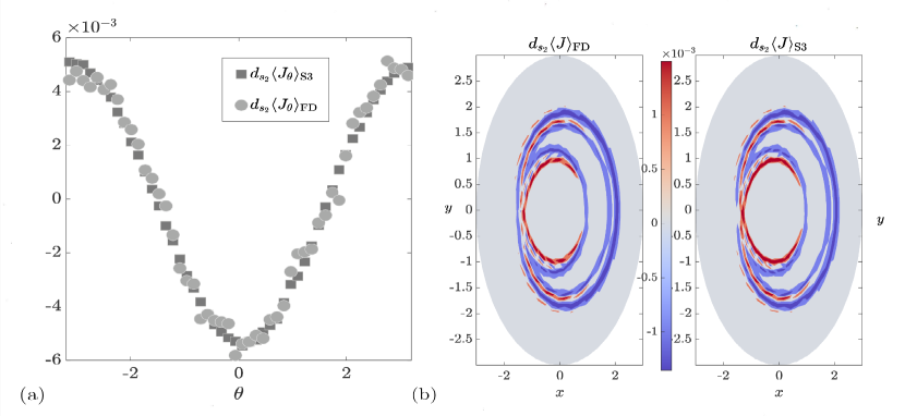
Figure 1: Comparison of the sensitivities computed with S3 to finite-difference for the solenoid map in Section 5.1. (a) $J$ is a set of two-variable nodal basis functions along $r$ and $\theta$ axes. (b) $J_{\theta}$ is a set of nodal basis functions along $\theta$ axis.

In this map, $r$ and $z$ directions form a basis for the stable subspace at each point (and the orthogonal $\theta$ direction forms a basis for the adjoint unstable subspace). Applying a perturbation to $s_{1}$ causes a stable perturbation, i.e., the unstable contribution is nonzero, since it affects only the $r$ coordinate. On the other hand, perturbing $s_{2}$ leads to a nonzero unstable contribution. A set of nodal basis functions along $r$ and $\theta$ is chosen to be the objective function. We use a more general S3 algorithm than presented in Section 3 that is derived under the SRB assumption but does not assume the existence of a density everywhere. In order to validate the S3 computation, we compare the sensitivities $(d\langle J\rangle/ds_{2})$ with finite-difference results generated using 10 billion Monte Carlo samples on the attractor. The sensitivities to the parameter $s_{2}$ are shown in Figure 1(a). In Figure 1(b), the objective function is a set of nodal basis functions along the $\theta$ direction. From Figures 1(a,b), we see close agreement between the sensitivities computed with (a more general version of) S3 and, finite-difference results, thus validating both the stable and unstable parts of the S3 algorithm.

5.2 Kuznetsov-Plykin map

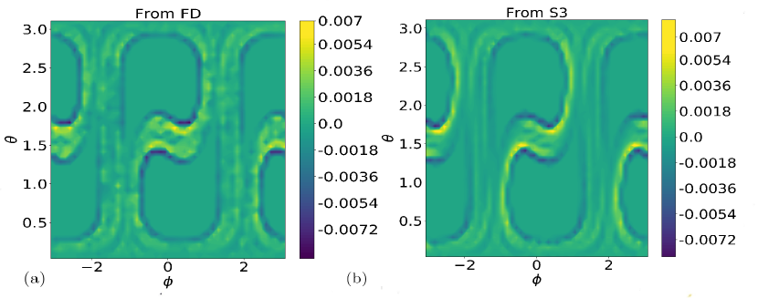
Figure 2: Comparison of the sensitivities of the nodal basis functions along the $\theta$ and $\phi$ axes to the parameter $s_{2}$ obtained for the Kuznetsov-Plykin attractor using (a) finite difference and (b) the S3 algorithm.

We consider as a second example the Kuznetsov-Plykin map as defined by Kuznetsov (2009), which describes a sequence of rotations and translations on the surface of the three-dimensional sphere. The two parameters we choose to vary are $s_{1}:=\epsilon$ and $s_{2}:=\mu$, which are defined by Kuznetsov (2009). The map is given by

$$\varphi_{n+1}^{s}(u)=f_{-1,-1}\circ f_{1,1}(u),$$ (20)

where $u=[x,y,z]^{T}$. For the function $f_{\cdot,\cdot}$ and further details regarding the hyperbolicity of the system, the reader is referred to Kuznetsov (2009). The probability distribution on the attractor again violates the smoothness condition in the derivation but satisfies the assumption of an existence of a density on the unstable manifolds. We again use a more general version of the S3 algorithm to compute the sensitivities as in the case of the solenoid map in Section 5.1. The objective function $J$ is a set of nodal basis functions along the $\theta$ and $\phi$ spherical coordinate axes. The finite-difference sensitivities were computed with the central difference around the reference value of $s_{2}=1$ by means of 10 billion independent samples on the attractor. The results from S3 agree well with finite-difference sensitivities as shown in Figure 2.

6 Conclusions

We have presented the tangent space-split sensitivity algorithm to compute the sensitivities of statistics to system parameters in chaotic dynamical systems. The algorithm requires the computation of a basis for the tangent and adjoint unstable subspaces along a long trajectory. The stable contribution to the overall sensitivity can be efficiently computed by a conventional tangent/adjoint computation just as in nonchaotic systems. The unstable contribution has been derived as an ergodic average that can be evaluated efficiently by using solutions to the Koopman tangent equation, which has been introduced. The numerical examples described in Section 5 do not satisfy the simplifying assumptions that were made in the derivation. However, they show close agreement with finite-difference results, suggesting that the ideas used in S3 can be extended to more general scenarios.

Acknowledgments

The authors gratefully acknowledge other summer program participants and our CTR hosts for many fruitful discussions. We would also like to thank our reviewer Dr. Patrick Blonigan for his valuable comments.

References

- Blonigan (2017) Blonigan P. 2017 Adjoint sensitivity analysis of chaotic dynamical systems with non-intrusive least squares shadowing. J. Comput. Phys. 348, 803–826.
- Chandramoorthy et al. (2017) Chandramoorthy, N. & Fernandez, P. & Talnikar, C. & Wang, Q. 2017 An Analysis of the Ensemble Adjoint Approach to Sensitivity Analysis in Chaotic Systems. AIAA Paper 2017-3799.
- Eyink et al. (2004) Eyink, G. L. & Haine, T. W. N. & Lea, D. J. 2004 Ruelle’s linear response formula, ensemble adjoint schemes and Lévy flights. Nonlinearity 17, 1867-1889
- Ginelli et al. (2013) Ginelli F. & Chaté H. & Livi R. & Politi A. 2013 Covariant lyapunov vectors. J. Phys. A: Math. Theor. 46, 254005.
- Grebogi et al. (1988) Grebogi C. & Ott E. & Yorke J. A. 1988 Unstable periodic orbits and the dimensions of multifractal chaotic attractors. Phys. Rev. A 37, 1711.
- Katok & Hasselblatt (1995) Katok, A. & Hasselblatt, B. 1995 Introduction to the modern theory of dynamical systems Cambridge university press 54
- Kuznetsov (2009) Kuznetsov S. P. 2009 A non-autonomous flow system with Plykin type attractor. Commun. Nonlinear Sci. 14, 3487–3491.
- Ni (2018) Ni A. 2018 Sensitivity analysis on chaotic dynamical systems by Non-Intrusive Least Squares Adjoint Shadowing (NILSAS) arXiv preprint 1801.08674
- Ni & Wang (2017) Ni A. and Wang Q. 2017 Sensitivity analysis on chaotic dynamical systems by Non-Intrusive Least Squares Shadowing (NILSS). J. Comput. Phys. 347, 56–77.
- Ruelle (1997) Ruelle, D. 1997 Differentiation of SRB states. Commun. Math. Phys. 187, 227–241.
- Wang (2014) Wang Q. 2014 Convergence of the least squares shadowing method for computing derivative of ergodic averages SIAM J. Numer. Anal.. 52, 156–170.
- Samareh (2001) Samareh J. 2001 Survey of shape parameterization techniques for high-fidelity multidisciplinary shape optimization AIAA J. 39, 877–884.
- Young (2002) Young L. S. 2002 What are SRB measures, and which dynamical systems have them?. J. Stat. Phys. 108(5-6), 733–754.