Scaling Theory of Quantum Ratchet
Keita Hamamoto1
Takamori Park1
Hiroaki Ishizuka1
Naoto Nagaosa1,2
1 Department of Applied Physics,
The University of Tokyo, Tokyo 113-8656, Japan
2 RIKEN Center for Emergent Matter Science (CEMS),
Wako, Saitama 351-0198, Japan
Abstract
The asymmetric responses of the system between the
external force of right and left directions are called ”nonreciprocal”.
There are many examples of nonreciprocal responses such
as the rectification by p-n junction.
However, the quantum mechanical wave does not
distinguish between the right and left directions as long as
the time-reversal symmetry is intact, and it is a highly
nontrivial issue how the nonreciprocal nature originates in
quantum systems.
Here we demonstrate by the quantum ratchet model, i.e.,
a quantum particle in an asymmetric periodic potential,
that the dissipation characterized by a dimensionless
coupling constant α 𝛼 \alpha T 𝑇 T μ 2 subscript 𝜇 2 \mu_{2} μ 2 ∼ T 6 / α − 4 similar-to subscript 𝜇 2 superscript 𝑇 6 𝛼 4 \mu_{2}\sim T^{6/\alpha-4} α < 1 𝛼 1 \alpha<1 μ 2 ∼ T 2 ( α − 1 ) similar-to subscript 𝜇 2 superscript 𝑇 2 𝛼 1 \mu_{2}\sim T^{2(\alpha-1)} α > 1 𝛼 1 \alpha>1 α c = 1 subscript 𝛼 𝑐 1 \alpha_{c}=1 μ 2 subscript 𝜇 2 \mu_{2} μ 2 ∼ T − 11 / 4 similar-to subscript 𝜇 2 superscript 𝑇 11 4 \mu_{2}\sim T^{-11/4} μ 2 subscript 𝜇 2 \mu_{2} v 𝑣 v F 𝐹 F T 𝑇 T
Chirality is one of the most basic subjects in whole sciences including
physics, chemistry, and biology Gardner ; Tokura Feynman Haddou ; Julicher Rousslett Faucheux Gorre
Quantum effects on the particle dynamics under the
nonreciprocal periodic potential V ( x ) 𝑉 𝑥 V(x) k 𝑘 k ε n ( k ) subscript 𝜀 𝑛 𝑘 \varepsilon_{n}(k) n 𝑛 n ε n ( k ) subscript 𝜀 𝑛 𝑘 \varepsilon_{n}(k) k 𝑘 k − k 𝑘 -k ε n ( k ) = ε n ( − k ) subscript 𝜀 𝑛 𝑘 subscript 𝜀 𝑛 𝑘 \varepsilon_{n}(k)=\varepsilon_{n}(-k) V ( x ) 𝑉 𝑥 V(x) Morimoto
Dynamics of a quantum Brownian particle in the periodic potential
with dissipation has been
the subject of intensive studies for a long term Weiss Caldeira ; LeggettRMP FeynmanVernon α 𝛼 \alpha α < α c = 1 𝛼 subscript 𝛼 𝑐 1 \alpha<\alpha_{c}=1 α > α c = 1 𝛼 subscript 𝛼 𝑐 1 \alpha>\alpha_{c}=1 Schmid ; GuineaPRL ; GuineaPRB ; Fisher ; Zwerger ; KanePRL ; KanePRB ; Furusaki μ 1 subscript 𝜇 1 \mu_{1} μ 1 ∝ 1 / α proportional-to subscript 𝜇 1 1 𝛼 \mu_{1}\propto 1/\alpha α < 1 𝛼 1 \alpha<1 μ 1 subscript 𝜇 1 \mu_{1} μ 1 ∼ T 2 ( α − 1 ) similar-to subscript 𝜇 1 superscript 𝑇 2 𝛼 1 \mu_{1}\sim T^{2(\alpha-1)} α > 1 𝛼 1 \alpha>1 T → 0 → 𝑇 0 T\to 0 α 𝛼 \alpha
Experimentally, the quantum ratchet effects in semiconductor heterostructure with
artificial asymmetric gating Exp1 Exp2 φ 𝜑 \varphi Exp3
Recently, the vortex flow resistance in a noncentrosymmetric superconductor is shown to
express a large directional dichroism at the low temperature Wakatsuki Hoshino
In this paper, we study the quantum dynamics of the particle in
an asymmetric periodic potential with Ohmic dissipation.
The form of the potential is for example taken as
V ( x ) = V 1 cos ( 2 π x a ) + V 2 sin ( 4 π x a ) 𝑉 𝑥 subscript 𝑉 1 2 𝜋 𝑥 𝑎 subscript 𝑉 2 4 𝜋 𝑥 𝑎 V(x)=V_{1}\cos\left(2\pi\frac{x}{a}\right)+V_{2}\sin\left(4\pi\frac{x}{a}\right) x → − x → 𝑥 𝑥 x\to-x Inst1 ; Inst2 ; Inst3 ; Inst4 ; Inst5 ; Vinokur ; Peguiron ; Peguiron2 Inst2 ; Inst3 ; Inst4 μ 2 subscript 𝜇 2 \mu_{2} Vinokur Peguiron ; Peguiron2 V ( x ) 𝑉 𝑥 V(x) μ 2 ∝ V 1 2 V 2 proportional-to subscript 𝜇 2 superscript subscript 𝑉 1 2 subscript 𝑉 2 \mu_{2}\propto V_{1}^{2}V_{2} v ( F ) + v ( − F ) ∝ V 1 2 V 2 proportional-to 𝑣 𝐹 𝑣 𝐹 superscript subscript 𝑉 1 2 subscript 𝑉 2 v(F)+v(-F)\propto V_{1}^{2}V_{2} t 1 subscript 𝑡 1 t_{1} t 2 subscript 𝑡 2 t_{2}
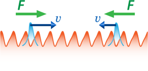
Figure 1: Schematic picture of the present system.
The particle wave packet under the ratchet potential is driven by the external force F 𝐹 F | v ( − F ) | ≠ | v ( F ) | 𝑣 𝐹 𝑣 𝐹 |v(-F)|\neq|v(F)|
Here, we rederive the general expression of the steady state velocity
as a function of external force F 𝐹 F V ( x ) 𝑉 𝑥 V(x) α < 1 𝛼 1 \alpha<1 α > 1 𝛼 1 \alpha>1 v ( F ) 𝑣 𝐹 v(F) μ n subscript 𝜇 𝑛 \mu_{n} FeynmanVernon J ( ω ) = η ω 𝐽 𝜔 𝜂 𝜔 J(\omega)=\eta\omega V ( x ) 𝑉 𝑥 V(x) T 𝑇 T F 𝐹 F Fisher ; Vinokur ; Eckern ; Peguiron ; Peguiron2 SM SM ℏ = k B = 1 Planck-constant-over-2-pi subscript 𝑘 𝐵 1 \hbar=k_{B}=1
The zeroth order in V 𝑉 V v ( 0 ) = F / η superscript 𝑣 0 𝐹 𝜂 v^{(0)}=F/\eta V 2 superscript 𝑉 2 V^{2} Fisher ; Vinokur ; Eckern ; Peguiron ; Peguiron2
v ( 2 ) superscript 𝑣 2 \displaystyle v^{(2)} = − 2 η ∫ 0 ∞ d t ∑ k k | V k | 2 sin [ F η k t ] absent 2 𝜂 superscript subscript 0 differential-d 𝑡 subscript 𝑘 𝑘 superscript subscript 𝑉 𝑘 2 𝐹 𝜂 𝑘 𝑡 \displaystyle=-\frac{2}{\eta}\int_{0}^{\infty}\mathrm{d}t\sum_{k}k\left|V_{k}\right|^{2}\sin\left[\frac{F}{\eta}kt\right]
× sin [ 1 π η k 2 Q 1 ( t ) ] exp [ − 1 π η k 2 Q 2 ( t ) ] . absent 1 𝜋 𝜂 superscript 𝑘 2 subscript 𝑄 1 𝑡 1 𝜋 𝜂 superscript 𝑘 2 subscript 𝑄 2 𝑡 \displaystyle\qquad\times\sin\left[\frac{1}{\pi\eta}k^{2}Q_{1}(t)\right]\exp\left[-\frac{1}{\pi\eta}k^{2}Q_{2}(t)\right]. (1)
Here V k subscript 𝑉 𝑘 V_{k} V ( x ) 𝑉 𝑥 V(x) k 𝑘 k 2 π / a 2 𝜋 𝑎 2\pi/{a} Q 1 subscript 𝑄 1 Q_{1} Q 2 subscript 𝑄 2 Q_{2} LeggettRMP
Q 1 ( t ) subscript 𝑄 1 𝑡 \displaystyle Q_{1}(t) = ∫ 0 ∞ d ω J ( ω ) η ω 2 sin ( ω t ) f ( ω / γ ) absent superscript subscript 0 differential-d 𝜔 𝐽 𝜔 𝜂 superscript 𝜔 2 𝜔 𝑡 𝑓 𝜔 𝛾 \displaystyle=\int_{0}^{\infty}\mathrm{d}\omega\frac{J(\omega)}{\eta\omega^{2}}\sin(\omega t)f(\omega/\gamma) (2)
Q 2 ( t ) subscript 𝑄 2 𝑡 \displaystyle Q_{2}(t) = ∫ 0 ∞ d ω J ( ω ) η ω 2 ( 1 − cos ( ω t ) ) coth ( ω 2 T ) f ( ω / γ ) . absent superscript subscript 0 differential-d 𝜔 𝐽 𝜔 𝜂 superscript 𝜔 2 1 𝜔 𝑡 hyperbolic-cotangent 𝜔 2 𝑇 𝑓 𝜔 𝛾 \displaystyle=\int_{0}^{\infty}\mathrm{d}\omega\frac{J(\omega)}{\eta\omega^{2}}\left(1-\cos(\omega t)\right)\coth\left(\frac{\omega}{2T}\right)f(\omega/\gamma). (3)
γ 𝛾 \gamma η 𝜂 \eta M 𝑀 M f 𝑓 f f ( ω / γ ) = e − ω / γ 𝑓 𝜔 𝛾 superscript 𝑒 𝜔 𝛾 f(\omega/\gamma)=e^{-\omega/\gamma} Peguiron ; Peguiron2 Vinokur F 𝐹 F Fisher k = ± 2 π a 𝑘 plus-or-minus 2 𝜋 𝑎 k=\pm\frac{2\pi}{a} V ( x ) 𝑉 𝑥 V(x) v ( 2 ) superscript 𝑣 2 v^{(2)} F 𝐹 F v ( 2 ) superscript 𝑣 2 v^{(2)} Q 1 subscript 𝑄 1 Q_{1} Q 2 subscript 𝑄 2 Q_{2} t , T − 1 ≫ γ − 1 much-greater-than 𝑡 superscript 𝑇 1
superscript 𝛾 1 t,T^{-1}\gg\gamma^{-1}
Q 1 ( t ) subscript 𝑄 1 𝑡 \displaystyle Q_{1}(t) = tan − 1 ( γ t ) → c o n s t . absent superscript 1 𝛾 𝑡 → 𝑐 𝑜 𝑛 𝑠 𝑡 \displaystyle=\tan^{-1}(\gamma t)\rightarrow const. (4)
Q 2 ( t ) subscript 𝑄 2 𝑡 \displaystyle Q_{2}(t) = log ( [ 1 + ( γ t ) 2 ] 1 / 2 | Γ ( 1 + T γ ) Γ ( 1 + T γ + i T t ) | 2 ) absent superscript delimited-[] 1 superscript 𝛾 𝑡 2 1 2 superscript Γ 1 𝑇 𝛾 Γ 1 𝑇 𝛾 𝑖 𝑇 𝑡 2 \displaystyle=\log\left(\left[1+(\gamma t)^{2}\right]^{1/2}\left|\frac{\Gamma(1+\frac{T}{\gamma})}{\Gamma(1+\frac{T}{\gamma}+iTt)}\right|^{2}\right)
→ log ( γ t ) + log ( sinh ( π T t ) π T t ) → absent 𝛾 𝑡 𝜋 𝑇 𝑡 𝜋 𝑇 𝑡 \displaystyle\rightarrow\log(\gamma t)+\log\left(\frac{\sinh(\pi Tt)}{\pi Tt}\right) (5)
with Γ ( ⋅ ) Γ ⋅ \Gamma(\cdot) F 𝐹 F n 𝑛 n v ( 2 ) superscript 𝑣 2 v^{(2)}
v ( 2 ) ∼ T 2 α − 1 − n F n similar-to superscript 𝑣 2 superscript 𝑇 2 𝛼 1 𝑛 superscript 𝐹 𝑛 \displaystyle v^{(2)}\sim T^{\frac{2}{\alpha}-1-n}F^{n} (6)
in the order of F n superscript 𝐹 𝑛 F^{n} n 𝑛 n
α = η a 2 2 π . 𝛼 𝜂 superscript 𝑎 2 2 𝜋 \displaystyle\alpha=\frac{\eta a^{2}}{2\pi}. (7)
In the third order of V 𝑉 V Fisher ; Vinokur ; Eckern ; Peguiron ; Peguiron2
v ( 3 ) superscript 𝑣 3 \displaystyle v^{(3)} = 4 η ∫ 0 ∞ d t 1 ∫ 0 ∞ d t 2 ∑ k 1 , k 2 , k 3 k 1 + k 2 + k 3 = 0 k 1 absent 4 𝜂 superscript subscript 0 differential-d subscript 𝑡 1 superscript subscript 0 differential-d subscript 𝑡 2 subscript subscript 𝑘 1 subscript 𝑘 2 subscript 𝑘 3
subscript 𝑘 1 subscript 𝑘 2 subscript 𝑘 3 0
subscript 𝑘 1 \displaystyle=\frac{4}{\eta}\int_{0}^{\infty}\mathrm{d}t_{1}\int_{0}^{\infty}\mathrm{d}t_{2}\sum_{\begin{subarray}{c}k_{1},k_{2},k_{3}\\
k_{1}+k_{2}+k_{3}=0\end{subarray}}k_{1}
× ( Re [ V k 1 V k 2 V k 3 ] sin [ F η ( k 1 t 1 − k 3 t 2 ) ] + Im [ V k 1 V k 2 V k 3 ] ( cos [ F η ( k 1 t 1 − k 3 t 2 ) ] − 1 ) ) absent subscript 𝑉 subscript 𝑘 1 subscript 𝑉 subscript 𝑘 2 subscript 𝑉 subscript 𝑘 3 𝐹 𝜂 subscript 𝑘 1 subscript 𝑡 1 subscript 𝑘 3 subscript 𝑡 2 subscript 𝑉 subscript 𝑘 1 subscript 𝑉 subscript 𝑘 2 subscript 𝑉 subscript 𝑘 3 𝐹 𝜂 subscript 𝑘 1 subscript 𝑡 1 subscript 𝑘 3 subscript 𝑡 2 1 \displaystyle\times\left(\real\left[V_{k_{1}}V_{k_{2}}V_{k_{3}}\right]\sin\left[\frac{F}{\eta}\left(k_{1}t_{1}-k_{3}t_{2}\right)\right]+\imaginary\left[V_{k_{1}}V_{k_{2}}V_{k_{3}}\right]\left(\cos\left[\frac{F}{\eta}\left(k_{1}t_{1}-k_{3}t_{2}\right)\right]-1\right)\right)
× exp [ 1 π η ( k 1 k 2 Q 2 ( t 1 ) + k 2 k 3 Q 2 ( t 2 ) + k 3 k 1 Q 2 ( t 1 + t 2 ) ) ] sin [ 1 π η k 1 k 2 Q 1 ( t 1 ) ] sin [ 1 π η ( k 2 k 3 Q 1 ( t 2 ) + k 3 k 1 Q 1 ( t 1 + t 2 ) ) ] . absent 1 𝜋 𝜂 subscript 𝑘 1 subscript 𝑘 2 subscript 𝑄 2 subscript 𝑡 1 subscript 𝑘 2 subscript 𝑘 3 subscript 𝑄 2 subscript 𝑡 2 subscript 𝑘 3 subscript 𝑘 1 subscript 𝑄 2 subscript 𝑡 1 subscript 𝑡 2 1 𝜋 𝜂 subscript 𝑘 1 subscript 𝑘 2 subscript 𝑄 1 subscript 𝑡 1 1 𝜋 𝜂 subscript 𝑘 2 subscript 𝑘 3 subscript 𝑄 1 subscript 𝑡 2 subscript 𝑘 3 subscript 𝑘 1 subscript 𝑄 1 subscript 𝑡 1 subscript 𝑡 2 \displaystyle\times\exp\left[\frac{1}{\pi\eta}\left(k_{1}k_{2}Q_{2}(t_{1})+k_{2}k_{3}Q_{2}(t_{2})+k_{3}k_{1}Q_{2}(t_{1}+t_{2})\right)\right]\sin\left[\frac{1}{\pi\eta}k_{1}k_{2}Q_{1}(t_{1})\right]\sin\left[\frac{1}{\pi\eta}\left(k_{2}k_{3}Q_{1}(t_{2})+k_{3}k_{1}Q_{1}(t_{1}+t_{2})\right)\right]. (8)
This result reduces to
the Scheidl-Vinokur’s result Vinokur F 2 superscript 𝐹 2 F^{2} v ( F ) + v ( − F ) 𝑣 𝐹 𝑣 𝐹 v(F)+v(-F) k = ± 2 π a , ± 4 π a 𝑘 plus-or-minus 2 𝜋 𝑎 plus-or-minus 4 𝜋 𝑎
k=\pm\frac{2\pi}{a},\pm\frac{4\pi}{a} Peguiron ; Peguiron2 5 − Q 2 ( t ) subscript 𝑄 2 𝑡 -Q_{2}(t) t 𝑡 t t 𝑡 t exp [ − π T t ] 𝜋 𝑇 𝑡 \exp[-\pi Tt] [ 0 , T − 1 ] 0 superscript 𝑇 1 [0,T^{-1}] T 𝑇 T
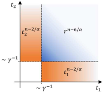
Figure 2:
Asymptotic behavior of the integrand of n 𝑛 n F 𝐹 F 8 t 1 subscript 𝑡 1 t_{1} t 2 subscript 𝑡 2 t_{2}
The dominant contribution to the integral originates from
( k 1 , k 2 , k 3 ) = ± 2 π a ( 1 , 1 , − 2 ) subscript 𝑘 1 subscript 𝑘 2 subscript 𝑘 3 plus-or-minus 2 𝜋 𝑎 1 1 2 (k_{1},k_{2},k_{3})=\pm\frac{2\pi}{a}(1,1,-2) ( r , θ ) 𝑟 𝜃 (r,\theta) F n ∫ r d r r n − 6 α ∼ T 6 α − 2 − n F n similar-to superscript 𝐹 𝑛 𝑟 differential-d 𝑟 superscript 𝑟 𝑛 6 𝛼 superscript 𝑇 6 𝛼 2 𝑛 superscript 𝐹 𝑛 F^{n}\int r\mathrm{d}r\ r^{n-\frac{6}{\alpha}}\sim T^{\frac{6}{\alpha}-2-n}F^{n} t 1 subscript 𝑡 1 t_{1} F n ∫ d t 2 t 2 n − 2 α ∼ T 2 α − 1 − n F n similar-to superscript 𝐹 𝑛 differential-d subscript 𝑡 2 superscript subscript 𝑡 2 𝑛 2 𝛼 superscript 𝑇 2 𝛼 1 𝑛 superscript 𝐹 𝑛 F^{n}\int\mathrm{d}t_{2}\ t_{2}^{n-\frac{2}{\alpha}}\sim T^{\frac{2}{\alpha}-1-n}F^{n} α < 4 𝛼 4 \alpha<4 k 1 , k 2 , k 3 subscript 𝑘 1 subscript 𝑘 2 subscript 𝑘 3
k_{1},k_{2},k_{3} SM 12 12 12
v ( 3 ) ∼ T 6 α − 2 − n F n similar-to superscript 𝑣 3 superscript 𝑇 6 𝛼 2 𝑛 superscript 𝐹 𝑛 \displaystyle v^{(3)}\sim T^{\frac{6}{\alpha}-2-n}F^{n} (9)
in the order of F n superscript 𝐹 𝑛 F^{n} n 𝑛 n
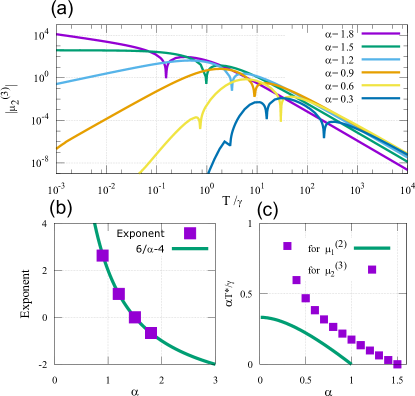
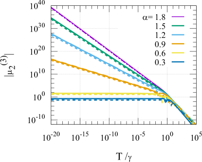
Figure 3: Temperature dependence of the second order mobility μ 2 ( 3 ) superscript subscript 𝜇 2 3 \mu_{2}^{(3)} μ 2 ( 3 ) superscript subscript 𝜇 2 3 \mu_{2}^{(3)} 8 V ( x ) = V 1 cos ( 2 π x / a ) + V 2 sin ( 4 π x / a ) 𝑉 𝑥 subscript 𝑉 1 2 𝜋 𝑥 𝑎 subscript 𝑉 2 4 𝜋 𝑥 𝑎 V(x)=V_{1}\cos(2\pi x/a)+V_{2}\sin(4\pi x/a) V 2 = V 1 / 4 subscript 𝑉 2 subscript 𝑉 1 4 V_{2}=V_{1}/4 α 𝛼 \alpha 6 / α − 4 6 𝛼 4 6/\alpha-4 − 11 / 4 11 4 -11/4 α > 1 𝛼 1 \alpha>1 μ 2 ( 3 ) superscript subscript 𝜇 2 3 \mu_{2}^{(3)} T ∗ ∗ superscript 𝑇 ∗ absent ∗ T^{\ast\ast} μ 2 ( 3 ) superscript subscript 𝜇 2 3 \mu_{2}^{(3)} μ 2 ( 3 ) ∝ T 6 / α − 4 proportional-to superscript subscript 𝜇 2 3 superscript 𝑇 6 𝛼 4 \mu_{2}^{(3)}\propto T^{6/\alpha-4} T ∗ superscript 𝑇 ∗ T^{\ast} μ 1 ( 2 ) superscript subscript 𝜇 1 2 \mu_{1}^{(2)} Scaling Theory of Quantum Ratchet
The numerical evaluation of second order mobility μ 2 ( 3 ) superscript subscript 𝜇 2 3 \mu_{2}^{(3)} 8 F 𝐹 F 3 9 0 < α < 3 / 2 0 𝛼 3 2 0<\alpha<3/2 μ 2 subscript 𝜇 2 \mu_{2} T = T ∗ ∼ γ 𝑇 superscript 𝑇 ∗ similar-to 𝛾 T=T^{\ast}\sim\gamma α > 1 𝛼 1 \alpha>1 μ 2 ( 3 ) superscript subscript 𝜇 2 3 \mu_{2}^{(3)} T ∗ ∗ superscript 𝑇 ∗ absent ∗ T^{\ast\ast} T ∗ superscript 𝑇 ∗ T^{\ast} V 𝑉 V V ( Λ ) = V ( Λ 0 ) ( Λ / Λ 0 ) 1 / α − 1 𝑉 Λ 𝑉 subscript Λ 0 superscript Λ subscript Λ 0 1 𝛼 1 V(\Lambda)=V(\Lambda_{0})(\Lambda/\Lambda_{0})^{1/\alpha-1} Λ Λ \Lambda Fisher Λ ∼ T similar-to Λ 𝑇 \Lambda\sim T V ( Λ 0 ) ( T ∗ ∗ / Λ 0 ) 1 / α − 1 ∼ T ∗ ∗ similar-to 𝑉 subscript Λ 0 superscript superscript 𝑇 ∗ absent ∗ subscript Λ 0 1 𝛼 1 superscript 𝑇 ∗ absent ∗ V(\Lambda_{0})(T^{\ast\ast}/\Lambda_{0})^{1/\alpha-1}\sim T^{\ast\ast}
The higher crossover temperature deduced from the peaks of Fig.3 3 μ 1 ( 2 ) superscript subscript 𝜇 1 2 \mu_{1}^{(2)} Scaling Theory of Quantum Ratchet μ 2 ( 3 ) superscript subscript 𝜇 2 3 \mu_{2}^{(3)} μ 1 ( 2 ) superscript subscript 𝜇 1 2 \mu_{1}^{(2)} μ 2 ( 3 ) superscript subscript 𝜇 2 3 \mu_{2}^{(3)} μ 1 ( 2 ) superscript subscript 𝜇 1 2 \mu_{1}^{(2)} μ 2 ( 3 ) superscript subscript 𝜇 2 3 \mu_{2}^{(3)} α 𝛼 \alpha
This low temperature dependence is in contrast to the saturating behavior discussed in ref.Vinokur Q 2 subscript 𝑄 2 Q_{2} μ 2 ( 3 ) superscript subscript 𝜇 2 3 \mu_{2}^{(3)} μ 2 ( 3 ) superscript subscript 𝜇 2 3 \mu_{2}^{(3)} α 𝛼 \alpha μ 2 ( 3 ) ∼ T − 11 / 4 similar-to superscript subscript 𝜇 2 3 superscript 𝑇 11 4 \mu_{2}^{(3)}\sim T^{-11/4} SM T − 17 / 6 superscript 𝑇 17 6 T^{-17/6} Vinokur f ( ω / γ ) 𝑓 𝜔 𝛾 f(\omega/\gamma) Vinokur
For α < 1 𝛼 1 \alpha<1 V 𝑉 V
v 𝑣 \displaystyle v = F η − F 2 / α − 1 f o < ( F / T ) − F 6 / α − 2 f e < ( F / T ) absent 𝐹 𝜂 superscript 𝐹 2 𝛼 1 superscript subscript 𝑓 𝑜 𝐹 𝑇 superscript 𝐹 6 𝛼 2 superscript subscript 𝑓 𝑒 𝐹 𝑇 \displaystyle=\frac{F}{\eta}-F^{2/\alpha-1}f_{o}^{<}(F/T)-F^{6/\alpha-2}f_{e}^{<}(F/T)
= F η − T 2 / α − 1 g o < ( F / T ) − T 6 / α − 2 g e < ( F / T ) absent 𝐹 𝜂 superscript 𝑇 2 𝛼 1 superscript subscript 𝑔 𝑜 𝐹 𝑇 superscript 𝑇 6 𝛼 2 superscript subscript 𝑔 𝑒 𝐹 𝑇 \displaystyle=\frac{F}{\eta}-T^{2/\alpha-1}g_{o}^{<}(F/T)-T^{6/\alpha-2}g_{e}^{<}(F/T) (10)
where f o < , g o < superscript subscript 𝑓 𝑜 superscript subscript 𝑔 𝑜
f_{o}^{<},g_{o}^{<} f e < , g e < superscript subscript 𝑓 𝑒 superscript subscript 𝑔 𝑒
f_{e}^{<},g_{e}^{<} F → 0 → 𝐹 0 F\to 0 t ≳ 1 / F greater-than-or-equivalent-to 𝑡 1 𝐹 t\gtrsim 1/F v 𝑣 v F n subscript 𝐹 𝑛 F_{n} v 𝑣 v T → 0 → 𝑇 0 T\to 0 v 𝑣 v T = 0 𝑇 0 T=0 10 g o < , g e < superscript subscript 𝑔 𝑜 superscript subscript 𝑔 𝑒
g_{o}^{<},g_{e}^{<} F / T 𝐹 𝑇 F/T F ≪ T much-less-than 𝐹 𝑇 F\ll T f o < , f e < superscript subscript 𝑓 𝑜 superscript subscript 𝑓 𝑒
f_{o}^{<},f_{e}^{<} f i < ( η ) = η 1 − 2 / α g i < ( η ) superscript subscript 𝑓 𝑖 𝜂 superscript 𝜂 1 2 𝛼 superscript subscript 𝑔 𝑖 𝜂 f_{i}^{<}(\eta)=\eta^{1-2/\alpha}g_{i}^{<}(\eta) i ∈ { e , o } 𝑖 𝑒 𝑜 i\in\{e,o\} V 2 subscript 𝑉 2 V_{2} g e < superscript subscript 𝑔 𝑒 g_{e}^{<} μ 2 subscript 𝜇 2 \mu_{2} μ 2 ∼ T 6 / α − 4 similar-to subscript 𝜇 2 superscript 𝑇 6 𝛼 4 \mu_{2}\sim T^{6/\alpha-4} n 𝑛 n μ n ∼ T 2 / α − n − 1 similar-to subscript 𝜇 𝑛 superscript 𝑇 2 𝛼 𝑛 1 \mu_{n}\sim T^{2/\alpha-n-1} μ n ∼ T 6 / α − 2 − n similar-to subscript 𝜇 𝑛 superscript 𝑇 6 𝛼 2 𝑛 \mu_{n}\sim T^{6/\alpha-2-n} α < 1 𝛼 1 \alpha<1 2 / ( n + 1 ) < α < 1 2 𝑛 1 𝛼 1 2/(n+1)<\alpha<1 6 / ( n + 2 ) < α < 1 6 𝑛 2 𝛼 1 6/(n+2)<\alpha<1 T → 0 → 𝑇 0 T\to 0 I 𝐼 I V 𝑉 V I ∼ V 6 g − 2 similar-to 𝐼 superscript 𝑉 6 𝑔 2 I\sim V^{6g-2} g 𝑔 g Feldman f e < superscript subscript 𝑓 𝑒 f_{e}^{<} 10 KanePRB ; KanePRL SM
From the viewpoint of the RG,
V 1 subscript 𝑉 1 V_{1} α < 1 𝛼 1 \alpha<1 α > 1 𝛼 1 \alpha>1 V 2 subscript 𝑉 2 V_{2} α < 4 𝛼 4 \alpha<4 α > 4 𝛼 4 \alpha>4 α 𝛼 \alpha 4 4 4 V 1 V 2 subscript 𝑉 1 subscript 𝑉 2 V_{1}V_{2} sin ( 2 π x a ) 2 𝜋 𝑥 𝑎 \sin\left(2\pi\frac{x}{a}\right) V 1 subscript 𝑉 1 V_{1} t 1 subscript 𝑡 1 t_{1} t 2 subscript 𝑡 2 t_{2} cos ( 2 π x / a ) 2 𝜋 𝑥 𝑎 \cos(2\pi x/a) sin ( 2 π x / a ) 2 𝜋 𝑥 𝑎 \sin(2\pi x/a) ∝ T 2 / α − 1 − n proportional-to absent superscript 𝑇 2 𝛼 1 𝑛 \propto T^{2/\alpha-1-n} v ( 3 ) superscript 𝑣 3 v^{(3)}
Now we turn to the case of α > 1 𝛼 1 \alpha>1 V 𝑉 V Schmid t 𝑡 t t 𝑡 t KanePRL ; KanePRB F 𝐹 F F 𝐹 F F 𝐹 F t 𝑡 t t ( F ) = t + γ F 𝑡 𝐹 𝑡 𝛾 𝐹 t(F)=t+\gamma F t ( F ) 𝑡 𝐹 t(F) v 𝑣 v
v 𝑣 \displaystyle v = t ( F ) 2 F 2 α − 1 f o > ( F / T ) absent 𝑡 superscript 𝐹 2 superscript 𝐹 2 𝛼 1 superscript subscript 𝑓 𝑜 𝐹 𝑇 \displaystyle=t(F)^{2}F^{2\alpha-1}f_{o}^{>}(F/T)
= t ( F ) 2 T 2 α − 1 g o > ( F / T ) , absent 𝑡 superscript 𝐹 2 superscript 𝑇 2 𝛼 1 superscript subscript 𝑔 𝑜 𝐹 𝑇 \displaystyle=t(F)^{2}T^{2\alpha-1}g_{o}^{>}(F/T), (11)
where g o > ( F / T ) superscript subscript 𝑔 𝑜 𝐹 𝑇 g_{o}^{>}(F/T) μ 2 subscript 𝜇 2 \mu_{2} T 2 ( α − 1 ) superscript 𝑇 2 𝛼 1 T^{2(\alpha-1)} μ 1 subscript 𝜇 1 \mu_{1} T → 0 → 𝑇 0 T\to 0
For the check of the scaling form Eq.(11 t 𝑡 t SM 11
Lastly, we comment on the array of resistively shunted josephson juntion model,
which is a direct generalization of the present system to higher dimensions.
This model, composed of the superconducting islands
connected by Josephson couplings with symmetric cosine potential and the
shunting Ohmic dissipation,
is a promising candidate to explain the low temperature behavior
of the thin film of granular superconductors Chakravarty ; Kapitulnik α = h / ( 4 e 2 R ) = 1 / z 0 𝛼 ℎ 4 superscript 𝑒 2 𝑅 1 subscript 𝑧 0 \alpha=h/(4e^{2}R)=1/z_{0} R 𝑅 R z 0 subscript 𝑧 0 z_{0} Chakravarty z 0 α > 1 subscript 𝑧 0 𝛼 1 z_{0}\alpha>1 n 𝑛 n n 𝑛 n R n ∼ T 2 / ( z 0 α ) − n − 1 similar-to subscript 𝑅 𝑛 superscript 𝑇 2 subscript 𝑧 0 𝛼 𝑛 1 R_{n}\sim T^{2/(z_{0}\alpha)-n-1} R n ∼ T 6 / ( z 0 α ) − n − 2 similar-to subscript 𝑅 𝑛 superscript 𝑇 6 subscript 𝑧 0 𝛼 𝑛 2 R_{n}\sim T^{6/(z_{0}\alpha)-n-2} 2 / ( n + 1 ) < z 0 α < 1 2 𝑛 1 subscript 𝑧 0 𝛼 1 2/(n+1)<z_{0}\alpha<1 6 / ( n + 2 ) < z 0 α < 1 6 𝑛 2 subscript 𝑧 0 𝛼 1 6/(n+2)<z_{0}\alpha<1
In summary, we have studied the role of dissipation in the
nonreciprocal transport of quantum particle in the asymmetric
periodic potential, i.e., quantum Ratchet model.
We have derived the general expression of the steady state velocity v 𝑣 v α 𝛼 \alpha F 𝐹 F T 𝑇 T V ( x ) 𝑉 𝑥 V(x) F 𝐹 F
Acknowledgment. —
We are grateful to A. J. Leggett for fruitful discussions.
N.N. was supported by Ministry
of Education, Culture, Sports, Science, and Technology
Nos. JP24224009 and JP26103006, the Impulsing Paradigm
Change through Disruptive Technologies Program of Council
for Science, Technology and Innovation (Cabinet Office,
Government of Japan), and JST CREST Grant Number JPMJCR1874, and JPMJCR16F1, Japan.
K.H. was supported by JSPS through a research fellowship for young
scientists and the Program for Leading Graduate Schools (MERIT)
References
(1)
M. Gardner, The Ambidextrous Universe. Left, Right and the Fall of Parity.
(Basic Books Inc., New York, 1964).
(2)
Y. Tokura and N. Nagaosa,
Nat. Comm. 9 , 3740 (2018)
(3)
R.P. Feynman, The Feynman Lectures on Physics, Vol. I.
(Addison-Wesley, 1963)
(4)
R. Ait-Haddou, and W. Herzog,
Cell Biochem. and Biophys. , 38 (2), 191 (2003).
(5)
F. Jülicher, A. Ajdari, and J. Prost,
Rev. of Mod. Phys. , 69 (4), 1269 (1997).
(6)
J. Rousselet, L. Salome, A. Ajdari, and J. Prost,
Nature , 370 , 446 (1994).
(7)
L. P. Faucheux, L. S. Bourdieu, P. D. Kaplan, and A. J. Libchaber,
Phys. Rev. Lett. , 74 , 1504 (1995).
(8)
L. Gorre, E. Ioannidis, and P. Silberzan,
Europhys. Lett. , 33 , 267 (1996).
(9)
T. Morimoto, and N. Nagaosa,
Sci. Rep. 8 , 2973 (2018).
(10)
U. Weiss, Quantum Dissipative Systems, (World Scientific, 2012).
(11)
A. O. Caldeira and A. J. Leggett,
Ann. Phys. (N.Y.) 149 , 374
(1983).
(12)
A. J. Leggett, S. Chakravarty, A. T. Dorsey, M. P. A. Fisher, A. Garg, and W. Zwerger,
Rev. Mod. Phys. 59 , 1 (1987).
(13)
R. P. Feynman and F. L. Vernon,
Ann. Phys. (N.Y.) 24 , 118
(1963).
(14)
A. Schmid,
Phys. Rev. Lett. 51 , 1506 (1983).
(15)
F. Guinea, V. Hakim, and A. Muramatsu,
Phys. Rev. Lett. 54 , 263 (1985).
(16)
F. Guinea,
Phys. Rev. B 32 , 7518 (1985).
(17)
M. P. A. Fisher and W. Zwerger,
Phys. Rev. B 32 , 6190 (1985).
(18)
W. Zwerger,
Phys. Rev. B 35 , 4737 (1987).
(19)
C.L. Kane and M.P.A. Fisher,
Phys. Rev. Lett. 68 , 1220 (1992).
(20)
C.L. Kane and M.P.A. Fisher,
Phys. Rev. B 46 , 15233 (1992).
(21)
A. Furusaki and N. Nagaosa,
Phys. Rev. B 47 , 4631 (1993).
(22)
H. Linke, T. E. Humphrey, A. Löfgren, A. O. Sushkov,
R. Newbury, R. P. Taylor, and P. Omling,
Science 286 , 2314 (1999).
(23)
J. B. Majer, J. Peguiron, M. Grifoni, M. Tusveld, and J. E. Mooij,
Phys. Rev. Lett. 90 , 056802 (2003).
(24)
R. Menditto, H. Sickinger, M. Weides, H. Kohlstedt, D. Koelle, R. Kleiner, and E. Goldobin,
Phys. Rev. E 94 , 042202 (2016).
(25)
R. Wakatsuki, Y. Saito, S. Hoshino, Y. M. Itahashi, T. Ideue, M. Ezawa, Y. Iwasa, N. Nagaosa,
Sci. Adv. 3 , e1602390 (2017).
(26)
S. Hoshino, R. Wakatsuki, K. Hamamoto, and N. Nagaosa,
Phys. Rev. B 98 , 054510 (2018).
(27)
P. Jung, J. G. Kissner, and P. Hänggi,
Phys. Rev. Lett. 76 , 3436 (1996).
(28)
P. Reimann, M. Grifoni, and P. Hänggi,
Phys. Rev. Lett. 79 , 10 (1997).
(29)
S. Yukawa, M. Kikuchi, G. Tatara, and H. Matsukawa,
J. Phys. Soc. Jpn. 66 , 2953 (1997).
(30)
G. Tatara, M. Kikuchi, S. Yukawa, and H. Matsukawa,
J. Phys. Soc. Jpn. 67 , 1090 (1998).
(31)
J. L. Mateos,
Phys. Rev. Lett. 84 , 258 (2000).
(32)
S. Scheidl, and V. M. Vinokur,
Phys. Rev. B 65 , 195305 (2002).
(33)
U. Eckern and F. Pelzer,
Europhys. Lett. 3 , 131 (1987).
(34)
J. Peguiron and M. Grifoni,
Phys. Rev. E 71 , 010101(R) (2005)
(35)
J. Peguiron and M. Grifoni,
Chem. Phys. 32 , 169 (2006)
(36)
See Supplemental Material at [URL will be inserted by publisher] for the derivations of eq.(Scaling Theory of Quantum Ratchet 8
(37)
D. E. Feldman, S. Scheidl, V. M. Vinokur,
Phys. Rev. Lett. 94 , 186809 (2005)
(38)
S. Chakravarty, G.-L. Ingold, S. Kivelson, and G. Zimanyi,
Phys. Rev. B 37 , 3283 (1987).
(39)
A. Kapitulunik, S. A. Kivelson, and B. Spivak,
arXiv , 1712:07215 (2017).
(40)
A. J. Thakkar and V. H. Smith,
Comp. Phys. Comm. , 10 , 73 (1975).
(41)
W. H. Press, S. A. Teukolsky, W. T. Vetterling, and B. P. Flannery,
Numerical Recipes 3rd Edition: The Art of Scientific Computing ,
(Cambridge University Press, Cambridge, 2007).
(42)
A. Schmid,
Journal of Low Temp. Phys. 49 , 609 (1982).
—Supplementary Materials—
Appendix A S1. Similarity to the Tomonaga-Lutinger liquid system
There are many similarities between the quantum Brownian particle studied in the main text and the Tomonaga-Luttinger liquid (TLL) KanePRB ; KanePRL α 𝛼 \alpha g 𝑔 g g = 1 / α 𝑔 1 𝛼 g=1/\alpha Schmid ; Fisher ; Peguiron α 𝛼 \alpha 1 / α 1 𝛼 1/\alpha
Since the problem of barriers in TLL have been extensively studied already, here
we will curtail detailed derivations and only discuss the similarities between the two models. The Euclidean action of a TLL is,
S = ∫ d x d τ v g 2 ( ( ∇ ϕ ) 2 + 1 v 2 ( ∂ τ ϕ ) 2 ) , 𝑆 𝑥 𝜏 𝑣 𝑔 2 superscript ∇ italic-ϕ 2 1 superscript 𝑣 2 superscript subscript 𝜏 italic-ϕ 2 S=\int\differential x\differential\tau\frac{vg}{2}\quantity((\nabla\phi)^{2}+\frac{1}{v^{2}}(\partial_{\tau}\phi)^{2}), (S1)
where g 𝑔 g 0 < g < 1 0 𝑔 1 0<g<1 g > 1 𝑔 1 g>1 t n subscript 𝑡 𝑛 t_{n} x = 0 𝑥 0 x=0 x ≠ 0 𝑥 0 x\neq 0
S [ ϕ ] = g ∑ ω n | ω n | | ϕ ( ω n ) | 2 + 1 2 ∑ n = − ∞ ∞ t n ∫ 0 β d τ e i 2 n π ϕ ( τ ) , 𝑆 delimited-[] italic-ϕ 𝑔 subscript subscript 𝜔 𝑛 subscript 𝜔 𝑛 superscript italic-ϕ subscript 𝜔 𝑛 2 1 2 superscript subscript 𝑛 subscript 𝑡 𝑛 superscript subscript 0 𝛽 𝜏 superscript 𝑒 𝑖 2 𝑛 𝜋 italic-ϕ 𝜏 S[\phi]=g\sum_{\omega_{n}}\absolutevalue{\omega_{n}}\absolutevalue{\phi(\omega_{n})}^{2}+\frac{1}{2}\sum_{n=-\infty}^{\infty}t_{n}\int_{0}^{\beta}\differential\tau e^{i2n\sqrt{\pi}\phi(\tau)}, (S2)
where ϕ ( τ ) = [ ϕ R ( τ , x = 0 ) − ϕ L ( τ , x = 0 ) ] / 2 italic-ϕ 𝜏 delimited-[] subscript italic-ϕ 𝑅 𝜏 𝑥
0 subscript italic-ϕ 𝐿 𝜏 𝑥
0 2 \phi(\tau)=[\phi_{R}(\tau,x=0)-\phi_{L}(\tau,x=0)]/2 x = 0 𝑥 0 x=0 t n subscript 𝑡 𝑛 t_{n} | n | 𝑛 \absolutevalue{n} n > 0 𝑛 0 n>0 n < 0 𝑛 0 n<0
A renormalization group analysis of the action shows that the hopping t n subscript 𝑡 𝑛 t_{n} g < 1 𝑔 1 g<1 a ( t ) 𝑎 𝑡 a(t) V ( t ) = ∂ t a ( t ) 𝑉 𝑡 subscript 𝑡 𝑎 𝑡 V(t)=\partial_{t}a(t) KanePRB
I ( 3 ) ( τ ) = − i 16 ∑ n 1 + n 2 + n 3 = 0 n 3 t n 1 t n 2 t n 3 ∫ 0 β d τ 1 ∫ 0 β d τ 2 P − 2 n 1 n 2 / g ( τ 1 − τ 2 ) P − 2 n 1 n 3 / g ( τ 1 − τ ) P − 2 n 2 n 3 / g ( τ 2 − τ ) , superscript 𝐼 3 𝜏 𝑖 16 subscript subscript 𝑛 1 subscript 𝑛 2 subscript 𝑛 3 0 subscript 𝑛 3 subscript 𝑡 subscript 𝑛 1 subscript 𝑡 subscript 𝑛 2 subscript 𝑡 subscript 𝑛 3 superscript subscript 0 𝛽 subscript 𝜏 1 superscript subscript 0 𝛽 subscript 𝜏 2 subscript 𝑃 2 subscript 𝑛 1 subscript 𝑛 2 𝑔 subscript 𝜏 1 subscript 𝜏 2 subscript 𝑃 2 subscript 𝑛 1 subscript 𝑛 3 𝑔 subscript 𝜏 1 𝜏 subscript 𝑃 2 subscript 𝑛 2 subscript 𝑛 3 𝑔 subscript 𝜏 2 𝜏 I^{(3)}(\tau)=-\frac{i}{16}\sum_{n_{1}+n_{2}+n_{3}=0}n_{3}t_{n_{1}}t_{n_{2}}t_{n_{3}}\int_{0}^{\beta}\differential\tau_{1}\int_{0}^{\beta}\differential\tau_{2}P_{-2n_{1}n_{2}/g}(\tau_{1}-\tau_{2})P_{-2n_{1}n_{3}/g}(\tau_{1}-\tau)P_{-2n_{2}n_{3}/g}(\tau_{2}-\tau), (S3)
where
P λ ( τ ) = ( π τ c / β sin ( π τ / β ) ) λ , subscript 𝑃 𝜆 𝜏 superscript 𝜋 subscript 𝜏 𝑐 𝛽 𝜋 𝜏 𝛽 𝜆 P_{\lambda}(\tau)=\quantity(\frac{\pi\tau_{c}/\beta}{\sin(\pi\tau/\beta)})^{\lambda}, (S4)
and τ c subscript 𝜏 𝑐 \tau_{c} t i = − ∞ → t i = t subscript 𝑡 𝑖 → subscript 𝑡 𝑖 𝑡 t_{i}=-\infty\rightarrow t_{i}=t t i = t → t i = − ∞ subscript 𝑡 𝑖 𝑡 → subscript 𝑡 𝑖 t_{i}=t\rightarrow t_{i}=-\infty
I ( 3 ) = 1 2 ∫ 0 ∞ d t 1 ∫ 0 ∞ d t 2 ∑ n 1 + n 2 + n 3 = 0 n i ∈ ℤ superscript 𝐼 3 1 2 superscript subscript 0 subscript 𝑡 1 superscript subscript 0 subscript 𝑡 2 subscript subscript 𝑛 1 subscript 𝑛 2 subscript 𝑛 3 0 subscript 𝑛 𝑖 ℤ
\displaystyle I^{(3)}=\frac{1}{2}\int_{0}^{\infty}\differential t_{1}\int_{0}^{\infty}\differential t_{2}\sum_{\begin{subarray}{c}n_{1}+n_{2}+n_{3}=0\\
n_{i}\in\mathbb{Z}\end{subarray}} n 1 t n 1 t n 2 t n 3 exp [ 2 g ( n 1 n 2 Q ( t 1 ) + n 2 n 3 Q ( t 2 ) + n 1 n 3 Q ( t 1 + t 2 ) ) ] subscript 𝑛 1 subscript 𝑡 subscript 𝑛 1 subscript 𝑡 subscript 𝑛 2 subscript 𝑡 subscript 𝑛 3 2 𝑔 subscript 𝑛 1 subscript 𝑛 2 𝑄 subscript 𝑡 1 subscript 𝑛 2 subscript 𝑛 3 𝑄 subscript 𝑡 2 subscript 𝑛 1 subscript 𝑛 3 𝑄 subscript 𝑡 1 subscript 𝑡 2 \displaystyle n_{1}t_{n_{1}}t_{n_{2}}t_{n_{3}}\exp[\frac{2}{g}\quantity(n_{1}n_{2}Q(t_{1})+n_{2}n_{3}Q(t_{2})+n_{1}n_{3}Q(t_{1}+t_{2}))]
× sin [ π g n 1 n 2 ] sin [ π g ( n 2 n 3 + n 1 n 3 ) ] sin [ V ( n 1 t 1 − n 3 t 2 ) ] , absent 𝜋 𝑔 subscript 𝑛 1 subscript 𝑛 2 𝜋 𝑔 subscript 𝑛 2 subscript 𝑛 3 subscript 𝑛 1 subscript 𝑛 3 𝑉 subscript 𝑛 1 subscript 𝑡 1 subscript 𝑛 3 subscript 𝑡 2 \displaystyle\times\sin\quantity[\frac{\pi}{g}n_{1}n_{2}]\sin\quantity[\frac{\pi}{g}(n_{2}n_{3}+n_{1}n_{3})]\sin\quantity[V(n_{1}t_{1}-n_{3}t_{2})], (S5)
where,
Q ( t ) = log ( t τ c ) + log ( sinh ( π T t ) π T t ) . 𝑄 𝑡 𝑡 subscript 𝜏 𝑐 𝜋 𝑇 𝑡 𝜋 𝑇 𝑡 Q(t)=\log\left(\frac{t}{\tau_{c}}\right)+\log\quantity(\frac{\sinh(\pi Tt)}{\pi Tt}). (S6)
Notice the similarities with the expression for the third order contribution in V 𝑉 V S5 Q 1 ( t ) , Q 2 ( t ) subscript 𝑄 1 𝑡 subscript 𝑄 2 𝑡
Q_{1}(t),Q_{2}(t) F 𝐹 F g 𝑔 g α 𝛼 \alpha g 𝑔 g 1 / g 1 𝑔 1/g g = 1 / α 𝑔 1 𝛼 g=1/\alpha
Note that in ref. Feldman I ∼ V 6 g − 2 similar-to 𝐼 superscript 𝑉 6 𝑔 2 I\sim V^{6g-2} v ∼ F 6 / α − 2 similar-to 𝑣 superscript 𝐹 6 𝛼 2 v\sim F^{6/\alpha-2} f e < superscript subscript 𝑓 𝑒 f_{e}^{<} 10
Appendix B S2. Conductance of a weak link in Tonomaga-Luttinger liquid
In this section, we numerically compute the first and third order conductance
of a weak link in an interacting TLL. We find that the current
is consistent with the scaling form,
I = T 2 / g − 1 g ( V T ) . 𝐼 superscript 𝑇 2 𝑔 1 𝑔 𝑉 𝑇 I=T^{2/g-1}g\left(\frac{V}{T}\right)\,. (S7)
We model a weak link or a high barrier in an interacting TLL by
adding a hopping term of strength t 𝑡 t g 𝑔 g KanePRB
S [ ϕ ] = g ∑ i ω n | ω n | | ϕ ( ω n ) | 2 + t ∫ d τ cos [ 2 π ϕ ( τ ) ] . 𝑆 delimited-[] italic-ϕ 𝑔 subscript 𝑖 subscript 𝜔 𝑛 subscript 𝜔 𝑛 superscript italic-ϕ subscript 𝜔 𝑛 2 𝑡 𝜏 2 𝜋 italic-ϕ 𝜏 S[\phi]=g\sum_{i\omega_{n}}\absolutevalue{\omega_{n}}\absolutevalue{\phi(\omega_{n})}^{2}+t\int\differential\tau\cos[2\sqrt{\pi}\phi(\tau)]\,. (S8)
Kane et. al. derived an expression up to second order in t 𝑡 t V 𝑉 V KanePRL
I ∝ t 2 ( 1 − e − β V ) P ~ ( V ) , proportional-to 𝐼 superscript 𝑡 2 1 superscript 𝑒 𝛽 𝑉 ~ 𝑃 𝑉 I\propto t^{2}(1-e^{-\beta V})\tilde{P}(V)\,, (S9)
where, P ~ ( V ) ~ 𝑃 𝑉 \tilde{P}(V) P ( t ) 𝑃 𝑡 P(t)
ln P ( t ) = − ∫ 0 ω c d ω 2 ω g [ coth ( ω 2 T ) ( 1 − cos ( ω t ) ) + i sin ( ω t ) ] . 𝑃 𝑡 superscript subscript 0 subscript 𝜔 𝑐 𝜔 2 𝜔 𝑔 hyperbolic-cotangent 𝜔 2 𝑇 1 𝜔 𝑡 𝑖 𝜔 𝑡 \ln P(t)=-\int_{0}^{\omega_{c}}\differential\omega\frac{2}{\omega g}\quantity[\coth\quantity(\frac{\omega}{2T})(1-\cos(\omega t))+i\sin(\omega t)]\,. (S10)
By introducting an exponential cutoff function e − ω / ω c superscript 𝑒 𝜔 subscript 𝜔 𝑐 e^{-\omega/\omega_{c}} P ( t ) 𝑃 𝑡 P(t)
P ( t ) = exp [ − 2 g ( i Q 1 ( t ) + Q 2 ( t ) ) ] , 𝑃 𝑡 2 𝑔 𝑖 subscript 𝑄 1 𝑡 subscript 𝑄 2 𝑡 P(t)=\exp\left[-\frac{2}{g}\left(iQ_{1}(t)+Q_{2}(t)\right)\right]\,, (S11)
where,
Q 1 ( t ) subscript 𝑄 1 𝑡 \displaystyle Q_{1}(t) = tan − 1 ( ω c t ) , absent superscript 1 subscript 𝜔 𝑐 𝑡 \displaystyle=\tan^{-1}(\omega_{c}t)\,, (S12)
Q 2 ( t ) subscript 𝑄 2 𝑡 \displaystyle Q_{2}(t) = 1 2 ln ( 1 + ω c 2 t 2 ) + ln ( sinh ( π T t ) π T t ) . absent 1 2 1 superscript subscript 𝜔 𝑐 2 superscript 𝑡 2 𝜋 𝑇 𝑡 𝜋 𝑇 𝑡 \displaystyle=\frac{1}{2}\ln(1+\omega_{c}^{2}t^{2})+\ln(\frac{\sinh(\pi Tt)}{\pi Tt})\,. (S13)
The Fourier transform, P ~ ( V ) ~ 𝑃 𝑉 \tilde{P}(V) Thakkar
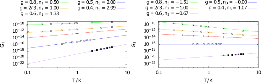
The first and third order conductances may be computed by approximating the
current, as a function of V 𝑉 V Recipes T 𝑇 T g < 1 𝑔 1 g<1
Figure S1 g 𝑔 g
G 1 subscript 𝐺 1 \displaystyle G_{1} ∝ T 2 / g − 2 , proportional-to absent superscript 𝑇 2 𝑔 2 \displaystyle\propto T^{2/g-2}\,, (S14)
G 3 subscript 𝐺 3 \displaystyle G_{3} ∝ G 1 T 2 ∝ T 2 / g − 4 . proportional-to absent subscript 𝐺 1 superscript 𝑇 2 proportional-to superscript 𝑇 2 𝑔 4 \displaystyle\propto\frac{G_{1}}{T^{2}}\propto T^{2/g-4}\,. (S15)
This is consistent with S7
I 𝐼 \displaystyle I = G 1 V + G 3 V 3 + 𝒪 ( V 5 ) absent subscript 𝐺 1 𝑉 subscript 𝐺 3 superscript 𝑉 3 𝒪 superscript 𝑉 5 \displaystyle=G_{1}V+G_{3}V^{3}+\mathcal{O}(V^{5})
= a T 2 / g − 2 V + b T 2 / g − 4 V 3 + 𝒪 ( V 5 ) absent 𝑎 superscript 𝑇 2 𝑔 2 𝑉 𝑏 superscript 𝑇 2 𝑔 4 superscript 𝑉 3 𝒪 superscript 𝑉 5 \displaystyle=aT^{2/g-2}V+bT^{2/g-4}V^{3}+\mathcal{O}(V^{5})
= T 2 / g − 1 g ( V T ) , absent superscript 𝑇 2 𝑔 1 𝑔 𝑉 𝑇 \displaystyle=T^{2/g-1}g\quantity(\frac{V}{T})\,, (S16)
where a , b ∈ ℝ 𝑎 𝑏
ℝ a,b\in\mathbb{R} g ( ⋅ ) 𝑔 ⋅ g(\cdot)
Figure S1: Log-log plot of the temperature dependence of the first (G 1 subscript 𝐺 1 G_{1} G 3 subscript 𝐺 3 G_{3} g = 0.4 , 0.5 , 0.6 , 2 / 3 , 𝑔 0.4 0.5 0.6 2 3
g=0.4\,,0.5\,,0.6\,,2/3\,, 0.8 0.8 0.8 n 1 , n 3 subscript 𝑛 1 subscript 𝑛 3
n_{1}\,,n_{3}
Appendix C S3. Derivation of equation (1) and (8)
In this section, we show the derivation of a general formula of the steady velocity in a tilted periodic potential with ohmic dissipation.
This is a direct generalization of the formula developed by Fisher and Zwerger Fisher V ( x ) = V 1 cos ( 2 π a x ) 𝑉 𝑥 subscript 𝑉 1 2 𝜋 𝑎 𝑥 V(x)=V_{1}\cos\left(\frac{2\pi}{a}x\right) Peguiron ; Peguiron2 v ( F ) + v ( − F ) 𝑣 𝐹 𝑣 𝐹 v(F)+v(-F) V ( x ) = V 1 cos ( 2 π a x ) + V 2 sin ( 4 π a x ) 𝑉 𝑥 subscript 𝑉 1 2 𝜋 𝑎 𝑥 subscript 𝑉 2 4 𝜋 𝑎 𝑥 V(x)=V_{1}\cos\left(\frac{2\pi}{a}x\right)+V_{2}\sin\left(\frac{4\pi}{a}x\right)
C.1 S3-1. Influence functional formalism
In this section, we briefly review the influence functional formalism just by following the Fisher and Zwerger. For the detail, see it and references therein.
In Feynmann-Vernon’s influence functional theory, the density matrix of system is obtained by taking a partial trace, by degrees of freedom of harmonic bath, of that of the total one;
ρ ( t ) = Tr bath [ ρ tot ( t ) ] . 𝜌 𝑡 subscript Tr bath delimited-[] subscript 𝜌 tot 𝑡 \rho(t)=\mathrm{Tr}_{\mathrm{bath}}\left[\rho_{\mathrm{tot}}(t)\right]. (S17)
In the coordinate representation,
⟨ q | ρ ( t ) | q ′ ⟩ = ∫ d q 0 ∫ d q 0 ′ ⟨ q 0 | ρ ( 0 ) | q 0 ′ ⟩ J ( q , q ′ , t | q 0 , q 0 ′ , 0 ) quantum-operator-product 𝑞 𝜌 𝑡 superscript 𝑞 ′ differential-d subscript 𝑞 0 differential-d superscript subscript 𝑞 0 ′ quantum-operator-product subscript 𝑞 0 𝜌 0 superscript subscript 𝑞 0 ′ 𝐽 𝑞 superscript 𝑞 ′ conditional 𝑡 subscript 𝑞 0 superscript subscript 𝑞 0 ′ 0
\Braket{q}{\rho(t)}{q^{\prime}}=\int\mathrm{d}q_{0}\int\mathrm{d}q_{0}^{\prime}\Braket{q_{0}}{\rho(0)}{q_{0}^{\prime}}J(q,q^{\prime},t|q_{0},q_{0}^{\prime},0) (S18)
with J 𝐽 J
J ( q , q ′ , t | q 0 , q 0 ′ , 0 ) = ∫ q 0 q 𝒟 q ∫ q 0 ′ q ′ 𝒟 q ′ exp [ i [ S ( q ) − S ( q ′ ) ] + i Φ ( q , q ′ ) ] . 𝐽 𝑞 superscript 𝑞 ′ conditional 𝑡 subscript 𝑞 0 superscript subscript 𝑞 0 ′ 0
superscript subscript subscript 𝑞 0 𝑞 𝒟 𝑞 superscript subscript subscript superscript 𝑞 ′ 0 superscript 𝑞 ′ 𝒟 superscript 𝑞 ′ 𝑖 delimited-[] 𝑆 𝑞 𝑆 superscript 𝑞 ′ 𝑖 Φ 𝑞 superscript 𝑞 ′ J(q,q^{\prime},t|q_{0},q_{0}^{\prime},0)=\int_{q_{0}}^{q}\mathcal{D}q\int_{q^{\prime}_{0}}^{q^{\prime}}\mathcal{D}q^{\prime}\exp\left[i\left[S(q)-S(q^{\prime})\right]+i\Phi(q,q^{\prime})\right]. (S19)
The action is
S ( q ) = ∫ 0 t d t ′ [ M 2 q ˙ 2 − U ( q ) ] 𝑆 𝑞 superscript subscript 0 𝑡 differential-d superscript 𝑡 ′ delimited-[] 𝑀 2 superscript ˙ 𝑞 2 𝑈 𝑞 S(q)=\int_{0}^{t}\mathrm{d}t^{\prime}\left[\frac{M}{2}\dot{q}^{2}-U(q)\right] (S20)
with tilted periodic potential;
U ( q ) = V ( q ) − F q = ∑ k V k e i k q − F q . 𝑈 𝑞 𝑉 𝑞 𝐹 𝑞 subscript 𝑘 subscript 𝑉 𝑘 superscript 𝑒 𝑖 𝑘 𝑞 𝐹 𝑞 U(q)=V(q)-Fq=\sum_{k}V_{k}e^{ikq}-Fq. (S21)
Momentum k 𝑘 k 2 π a 2 𝜋 𝑎 \frac{2\pi}{a} Φ Φ \Phi
i Φ ( x , y ) = 𝑖 Φ 𝑥 𝑦 absent \displaystyle i\Phi(x,y)= − i ∫ 0 t d t ′ ∫ t ′ t d s 2 x ( t ′ ) α I ( s − t ′ ) y ( s ) − i M ( Δ ω ) 2 ∫ 0 t d t ′ x ( t ′ ) y ( t ′ ) 𝑖 superscript subscript 0 𝑡 differential-d superscript 𝑡 ′ superscript subscript superscript 𝑡 ′ 𝑡 differential-d 𝑠 2 𝑥 superscript 𝑡 ′ subscript 𝛼 𝐼 𝑠 superscript 𝑡 ′ 𝑦 𝑠 𝑖 𝑀 superscript Δ 𝜔 2 superscript subscript 0 𝑡 differential-d superscript 𝑡 ′ 𝑥 superscript 𝑡 ′ 𝑦 superscript 𝑡 ′ \displaystyle-i\int_{0}^{t}\mathrm{d}t^{\prime}\int_{t^{\prime}}^{t}\mathrm{d}s\ 2x(t^{\prime})\alpha_{I}(s-t^{\prime})y(s)-iM(\Delta\omega)^{2}\int_{0}^{t}\mathrm{d}t^{\prime}x(t^{\prime})y(t^{\prime})
− ∫ 0 t d t ′ ∫ 0 t ′ d s y ( t ′ ) α R ( t ′ − s ) y ( s ) superscript subscript 0 𝑡 differential-d superscript 𝑡 ′ superscript subscript 0 superscript 𝑡 ′ differential-d 𝑠 𝑦 superscript 𝑡 ′ subscript 𝛼 𝑅 superscript 𝑡 ′ 𝑠 𝑦 𝑠 \displaystyle-\int_{0}^{t}\mathrm{d}t^{\prime}\int_{0}^{t^{\prime}}\mathrm{d}s\ y(t^{\prime})\alpha_{R}(t^{\prime}-s)y(s) (S22)
with
x = ( q + q ′ ) / 2 , y = q − q ′ . formulae-sequence 𝑥 𝑞 superscript 𝑞 ′ 2 𝑦 𝑞 superscript 𝑞 ′ x=(q+q^{\prime})/2,\qquad y=q-q^{\prime}. (S23)
The integral kernels are
α I ( t ) subscript 𝛼 𝐼 𝑡 \displaystyle\alpha_{I}(t) = − ∫ 0 ∞ d ω π J ( ω ) sin ω t absent superscript subscript 0 d 𝜔 𝜋 𝐽 𝜔 𝜔 𝑡 \displaystyle=-\int_{0}^{\infty}\frac{\mathrm{d}\omega}{\pi}J(\omega)\sin\omega t (S24)
α R ( t ) subscript 𝛼 𝑅 𝑡 \displaystyle\alpha_{R}(t) = ∫ 0 ∞ d ω π J ( ω ) cos ω t coth ( ℏ ω 2 T ) absent superscript subscript 0 d 𝜔 𝜋 𝐽 𝜔 𝜔 𝑡 hyperbolic-cotangent Planck-constant-over-2-pi 𝜔 2 𝑇 \displaystyle=\int_{0}^{\infty}\frac{\mathrm{d}\omega}{\pi}J(\omega)\cos\omega t\coth\left(\frac{\hbar\omega}{2T}\right) (S25)
1 2 M ( Δ ω ) 2 1 2 𝑀 superscript Δ 𝜔 2 \displaystyle\frac{1}{2}M(\Delta\omega)^{2} = ∫ 0 ∞ d ω π J ( ω ) ω absent superscript subscript 0 d 𝜔 𝜋 𝐽 𝜔 𝜔 \displaystyle=\int_{0}^{\infty}\frac{\mathrm{d}\omega}{\pi}\frac{J(\omega)}{\omega} (S26)
The specialized expression for the Ohmic dissipation J ( ω ) = η ω 𝐽 𝜔 𝜂 𝜔 J(\omega)=\eta\omega
i Φ ( x , y ) = i η ∫ 0 t d t ′ x ( t ′ ) y ˙ ( t ′ ) − i η x ( t ) y ( t ) − S 2 [ y ] 𝑖 Φ 𝑥 𝑦 𝑖 𝜂 superscript subscript 0 𝑡 differential-d superscript 𝑡 ′ 𝑥 superscript 𝑡 ′ ˙ 𝑦 superscript 𝑡 ′ 𝑖 𝜂 𝑥 𝑡 𝑦 𝑡 subscript 𝑆 2 delimited-[] 𝑦 i\Phi(x,y)=i\eta\int_{0}^{t}\mathrm{d}t^{\prime}x(t^{\prime})\dot{y}(t^{\prime})-i\eta x(t)y(t)-S_{2}[y] (S27)
with
S 2 [ y ] = ∫ 0 t d t ′ ∫ 0 t ′ d s y ( t ′ ) α R ( t ′ − s ) y ( s ) . subscript 𝑆 2 delimited-[] 𝑦 superscript subscript 0 𝑡 differential-d superscript 𝑡 ′ superscript subscript 0 superscript 𝑡 ′ differential-d 𝑠 𝑦 superscript 𝑡 ′ subscript 𝛼 𝑅 superscript 𝑡 ′ 𝑠 𝑦 𝑠 S_{2}[y]=\int_{0}^{t}\mathrm{d}t^{\prime}\int_{0}^{t^{\prime}}\mathrm{d}s\ y(t^{\prime})\alpha_{R}(t^{\prime}-s)y(s). (S28)
The potential term in action is nonlinear therefore we expand as
exp [ i [ S ( q ) − S ( q ′ ) ] ] 𝑖 delimited-[] 𝑆 𝑞 𝑆 superscript 𝑞 ′ \displaystyle\exp\left[i\left[S(q)-S(q^{\prime})\right]\right] = exp [ i ∫ 0 t d t ′ M 2 ( q ˙ 2 − q ˙ ′ 2 ) − ∑ k V k e i k q + F q + ∑ k V k e i k q ′ − F q ′ ] absent 𝑖 superscript subscript 0 𝑡 differential-d superscript 𝑡 ′ 𝑀 2 superscript ˙ 𝑞 2 superscript ˙ 𝑞 ′ 2
subscript 𝑘 subscript 𝑉 𝑘 superscript 𝑒 𝑖 𝑘 𝑞 𝐹 𝑞 subscript 𝑘 subscript 𝑉 𝑘 superscript 𝑒 𝑖 𝑘 superscript 𝑞 ′ 𝐹 superscript 𝑞 ′ \displaystyle=\exp\left[i\int_{0}^{t}\mathrm{d}t^{\prime}\ \frac{M}{2}\left(\dot{q}^{2}-\dot{q}^{\prime 2}\right)-\sum_{k}V_{k}e^{ikq}+Fq+\sum_{k}V_{k}e^{ikq^{\prime}}-Fq^{\prime}\right]
= exp [ i ∫ 0 t d t ′ M x ˙ y ˙ + F y ] absent 𝑖 superscript subscript 0 𝑡 differential-d superscript 𝑡 ′ 𝑀 ˙ 𝑥 ˙ 𝑦 𝐹 𝑦 \displaystyle=\exp\left[i\int_{0}^{t}\mathrm{d}t^{\prime}\ M\dot{x}\dot{y}+Fy\right]
× [ ∑ n = 0 ∞ ( − i ) n ∫ 0 t d t 1 ⋯ ∫ 0 t n − 1 d t n ∑ k 1 k 2 ⋯ k n ( ∏ i = 1 n V k i ) exp [ − i ∫ 0 t d t ′ ρ ( t ′ ) q ( t ′ ) ] ] absent delimited-[] superscript subscript 𝑛 0 superscript 𝑖 𝑛 superscript subscript 0 𝑡 differential-d subscript 𝑡 1 ⋯ superscript subscript 0 subscript 𝑡 𝑛 1 differential-d subscript 𝑡 𝑛 subscript subscript 𝑘 1 subscript 𝑘 2 ⋯ subscript 𝑘 𝑛 superscript subscript product 𝑖 1 𝑛 subscript 𝑉 subscript 𝑘 𝑖 𝑖 superscript subscript 0 𝑡 differential-d superscript 𝑡 ′ 𝜌 superscript 𝑡 ′ 𝑞 superscript 𝑡 ′ \displaystyle\qquad\times\left[\sum_{n=0}^{\infty}(-i)^{n}\int_{0}^{t}\mathrm{d}t_{1}\cdots\int_{0}^{t_{n-1}}\mathrm{d}t_{n}\sum_{k_{1}k_{2}\cdots k_{n}}\left(\prod_{i=1}^{n}V_{k_{i}}\right)\exp\left[-i\int_{0}^{t}\mathrm{d}t^{\prime}{\rho(t^{\prime})q(t^{\prime})}\right]\right]
× [ ∑ m = 0 ∞ i m ∫ 0 t d t 1 ′ ⋯ ∫ 0 t m − 1 ′ d t m ′ ∑ k 1 ′ k 2 ′ ⋯ k m ′ ( ∏ i = 1 m V k i ′ ) exp [ + i ∫ 0 t d t ′ ρ ′ ( t ′ ) q ( t ′ ) ] ] absent delimited-[] superscript subscript 𝑚 0 superscript 𝑖 𝑚 superscript subscript 0 𝑡 differential-d subscript superscript 𝑡 ′ 1 ⋯ superscript subscript 0 subscript superscript 𝑡 ′ 𝑚 1 differential-d subscript superscript 𝑡 ′ 𝑚 subscript subscript superscript 𝑘 ′ 1 subscript superscript 𝑘 ′ 2 ⋯ subscript superscript 𝑘 ′ 𝑚 superscript subscript product 𝑖 1 𝑚 subscript 𝑉 subscript superscript 𝑘 ′ 𝑖 𝑖 superscript subscript 0 𝑡 differential-d superscript 𝑡 ′ superscript 𝜌 ′ superscript 𝑡 ′ 𝑞 superscript 𝑡 ′ \displaystyle\qquad\times\left[\sum_{m=0}^{\infty}i^{m}\int_{0}^{t}\mathrm{d}t^{\prime}_{1}\cdots\int_{0}^{t^{\prime}_{m-1}}\mathrm{d}t^{\prime}_{m}\sum_{k^{\prime}_{1}k^{\prime}_{2}\cdots k^{\prime}_{m}}\left(\prod_{i=1}^{m}V_{k^{\prime}_{i}}\right)\exp\left[+i\int_{0}^{t}\mathrm{d}t^{\prime}{\rho^{\prime}(t^{\prime})q(t^{\prime})}\right]\right] (S29)
where we have defined two ”charge” densities
ρ ( t ′ ) = − ∑ i = 1 n k i δ ( t ′ − t i ) , ρ ′ ( t ′ ) = ∑ i = 1 m k i ′ δ ( t ′ − t i ′ ) . formulae-sequence 𝜌 superscript 𝑡 ′ superscript subscript 𝑖 1 𝑛 subscript 𝑘 𝑖 𝛿 superscript 𝑡 ′ subscript 𝑡 𝑖 superscript 𝜌 ′ superscript 𝑡 ′ superscript subscript 𝑖 1 𝑚 subscript superscript 𝑘 ′ 𝑖 𝛿 superscript 𝑡 ′ subscript superscript 𝑡 ′ 𝑖 \rho(t^{\prime})=-\sum_{i=1}^{n}k_{i}\delta(t^{\prime}-t_{i}),\qquad\rho^{\prime}(t^{\prime})=\sum_{i=1}^{m}k^{\prime}_{i}\delta(t^{\prime}-t^{\prime}_{i}). (S30)
Thus the probablity density is written as
P ( x , t ) 𝑃 𝑥 𝑡 \displaystyle P(x,t) = ⟨ x | ρ ( t ) | x ⟩ absent quantum-operator-product 𝑥 𝜌 𝑡 𝑥 \displaystyle=\Braket{x}{\rho(t)}{x}
= ∑ n , m = 0 ∞ ( − i ) n i m ∫ 0 t d t 1 ⋯ ∫ 0 t n − 1 d t n ∫ 0 t d t 1 ′ ⋯ ∫ 0 t m − 1 ′ d t m ′ ∑ k 1 ⋯ k n , k 1 ′ ⋯ k n ′ ( ∏ i = 1 n V k i ) ( ∏ i = 1 m V k i ′ ) absent superscript subscript 𝑛 𝑚
0 superscript 𝑖 𝑛 superscript 𝑖 𝑚 superscript subscript 0 𝑡 differential-d subscript 𝑡 1 ⋯ superscript subscript 0 subscript 𝑡 𝑛 1 differential-d subscript 𝑡 𝑛 superscript subscript 0 𝑡 differential-d subscript superscript 𝑡 ′ 1 ⋯ superscript subscript 0 subscript superscript 𝑡 ′ 𝑚 1 differential-d subscript superscript 𝑡 ′ 𝑚 subscript subscript 𝑘 1 ⋯ subscript 𝑘 𝑛 superscript subscript 𝑘 1 ′ ⋯ subscript superscript 𝑘 ′ 𝑛
superscript subscript product 𝑖 1 𝑛 subscript 𝑉 subscript 𝑘 𝑖 superscript subscript product 𝑖 1 𝑚 subscript 𝑉 subscript superscript 𝑘 ′ 𝑖 \displaystyle=\sum_{n,m=0}^{\infty}(-i)^{n}i^{m}\int_{0}^{t}\mathrm{d}t_{1}\cdots\int_{0}^{t_{n-1}}\mathrm{d}t_{n}\int_{0}^{t}\mathrm{d}t^{\prime}_{1}\cdots\int_{0}^{t^{\prime}_{m-1}}\mathrm{d}t^{\prime}_{m}\sum_{k_{1}\cdots k_{n},k_{1}^{\prime}\cdots k^{\prime}_{n}}\left(\prod_{i=1}^{n}V_{k_{i}}\right)\left(\prod_{i=1}^{m}V_{k^{\prime}_{i}}\right)
× ∫ d x 0 ∫ d y 0 ′ ⟨ x 0 + y 0 2 | ρ ( 0 ) | x 0 − y 0 2 ⟩ G \displaystyle\times\int\mathrm{d}x_{0}\int\mathrm{d}y_{0}^{\prime}\Braket{x_{0}+\frac{y_{0}}{2}}{\rho(0)}{x_{0}-\frac{y_{0}}{2}}G (S31)
with G 𝐺 G
G 𝐺 \displaystyle G = ∫ x 0 x 𝒟 x ∫ y 0 0 𝒟 y exp [ i ∫ 0 t d t ′ M x ˙ y ˙ + F y − ( ρ − ρ ′ ) x − 1 2 ( ρ + ρ ′ ) y + η x y ˙ ] absent superscript subscript subscript 𝑥 0 𝑥 𝒟 𝑥 superscript subscript subscript 𝑦 0 0 𝒟 𝑦 𝑖 superscript subscript 0 𝑡 differential-d superscript 𝑡 ′ 𝑀 ˙ 𝑥 ˙ 𝑦 𝐹 𝑦 𝜌 superscript 𝜌 ′ 𝑥 1 2 𝜌 superscript 𝜌 ′ 𝑦 𝜂 𝑥 ˙ 𝑦 \displaystyle=\int_{x_{0}}^{x}\mathcal{D}x\int_{y_{0}}^{0}\mathcal{D}y\exp\left[i\int_{0}^{t}\mathrm{d}t^{\prime}\ M\dot{x}\dot{y}+Fy-(\rho-\rho^{\prime})x-\frac{1}{2}(\rho+\rho^{\prime})y+\eta x\dot{y}\right]
exp [ − i η x ( t ) y ( t ) − S 2 [ y ] ] 𝑖 𝜂 𝑥 𝑡 𝑦 𝑡 subscript 𝑆 2 delimited-[] 𝑦 \displaystyle\qquad\qquad\exp\left[-i\eta x(t)y(t)-S_{2}[y]\right]
= A ( t ) exp [ i ∫ 0 t d t ′ [ F − 1 2 ( ρ + ρ ′ ) ] y ] exp [ − M x y ˙ | 0 t − S 2 [ y ] ] absent 𝐴 𝑡 𝑖 superscript subscript 0 𝑡 differential-d superscript 𝑡 ′ delimited-[] 𝐹 1 2 𝜌 superscript 𝜌 ′ 𝑦 evaluated-at 𝑀 𝑥 ˙ 𝑦 0 𝑡 subscript 𝑆 2 delimited-[] 𝑦 \displaystyle=A(t)\exp\left[i\int_{0}^{t}\mathrm{d}t^{\prime}\ \left[F-\frac{1}{2}(\rho+\rho^{\prime})\right]y\right]\exp\left[-M\left.x\dot{y}\right|_{0}^{t}-S_{2}[y]\right] (S32)
Now, coordinate y 𝑦 y M y ¨ − η y ˙ = ρ ′ − ρ . 𝑀 ¨ 𝑦 𝜂 ˙ 𝑦 superscript 𝜌 ′ 𝜌 M\ddot{y}-\eta\dot{y}=\rho^{\prime}-\rho. y ( t ′ = t ) = 0 𝑦 superscript 𝑡 ′ 𝑡 0 y(t^{\prime}=t)=0 A ( t ) = M 2 π d ( t ) 𝐴 𝑡 𝑀 2 𝜋 𝑑 𝑡 A(t)=\frac{M}{2\pi d(t)} d ( t ′ ) = γ − 1 ( 1 − e − γ t ′ ) 𝑑 superscript 𝑡 ′ superscript 𝛾 1 1 superscript 𝑒 𝛾 superscript 𝑡 ′ d(t^{\prime})=\gamma^{-1}(1-e^{-\gamma t^{\prime}})
By the same argument as in Fisher-Zwerger Fisher t → ∞ → 𝑡 t\rightarrow\infty
∫ 0 t d t ′ ( ρ − ρ ′ ) = 0 ⇔ ∑ i = 1 n k i + ∑ i = 1 m k i ′ = 0 formulae-sequence superscript subscript 0 𝑡 differential-d superscript 𝑡 ′ 𝜌 superscript 𝜌 ′ 0 ⇔
superscript subscript 𝑖 1 𝑛 subscript 𝑘 𝑖 superscript subscript 𝑖 1 𝑚 subscript superscript 𝑘 ′ 𝑖 0 \int_{0}^{t}\mathrm{d}t^{\prime}(\rho-\rho^{\prime})=0\qquad\Leftrightarrow\qquad\sum_{i=1}^{n}k_{i}+\sum_{i=1}^{m}k^{\prime}_{i}=0 (S33)
which is the ”momentum conservation” discussed by Scheidl and VinokurVinokur
The differential equation M y ¨ − η y ˙ = ρ ′ − ρ 𝑀 ¨ 𝑦 𝜂 ˙ 𝑦 superscript 𝜌 ′ 𝜌 M\ddot{y}-\eta\dot{y}=\rho^{\prime}-\rho y ( 0 ) = y 0 , y ( t ) = 0 formulae-sequence 𝑦 0 subscript 𝑦 0 𝑦 𝑡 0 y(0)=y_{0},y(t)=0
y ( t ′ ) 𝑦 superscript 𝑡 ′ \displaystyle y(t^{\prime}) = y h ( t ′ ) + y p ( t ′ ) absent subscript 𝑦 ℎ superscript 𝑡 ′ subscript 𝑦 𝑝 superscript 𝑡 ′ \displaystyle=y_{h}(t^{\prime})+y_{p}(t^{\prime})
y h ( t ′ ) subscript 𝑦 ℎ superscript 𝑡 ′ \displaystyle y_{h}(t^{\prime}) = y 0 γ d ( t ) [ 1 − e − γ ( t − t ′ ) ] absent subscript 𝑦 0 𝛾 𝑑 𝑡 delimited-[] 1 superscript 𝑒 𝛾 𝑡 superscript 𝑡 ′ \displaystyle=\frac{y_{0}}{\gamma d(t)}\left[1-e^{-\gamma(t-t^{\prime})}\right]
y p ( t ′ ) subscript 𝑦 𝑝 superscript 𝑡 ′ \displaystyle y_{p}(t^{\prime}) = − 1 η [ ∑ i = 1 n k i h ( t ′ − t i ) + ∑ i = 1 m k i ′ h ( t ′ − t i ′ ) ] absent 1 𝜂 delimited-[] superscript subscript 𝑖 1 𝑛 subscript 𝑘 𝑖 ℎ superscript 𝑡 ′ subscript 𝑡 𝑖 superscript subscript 𝑖 1 𝑚 subscript superscript 𝑘 ′ 𝑖 ℎ superscript 𝑡 ′ subscript superscript 𝑡 ′ 𝑖 \displaystyle=-\frac{1}{\eta}\left[\sum_{i=1}^{n}k_{i}h(t^{\prime}-t_{i})+\sum_{i=1}^{m}k^{\prime}_{i}h(t^{\prime}-t^{\prime}_{i})\right] (S34)
with γ = η / M 𝛾 𝜂 𝑀 \gamma=\eta/M h ( t ′ ) = e γ t ′ Θ ( − t ′ ) + Θ ( t ′ ) ℎ superscript 𝑡 ′ superscript 𝑒 𝛾 superscript 𝑡 ′ Θ superscript 𝑡 ′ Θ superscript 𝑡 ′ h(t^{\prime})=e^{\gamma t^{\prime}}\Theta(-t^{\prime})+\Theta(t^{\prime})
C.2 S3-2. Mobility
As shown by Fisher and Zwerger, the nonlinear mobility of the system is
μ μ 0 = 1 − lim t → ∞ 1 F t ⟨ ∫ 0 t d t ′ 1 2 ( ρ + ρ ′ ) ⟩ . 𝜇 subscript 𝜇 0 1 subscript → 𝑡 1 𝐹 𝑡 expectation superscript subscript 0 𝑡 differential-d superscript 𝑡 ′ 1 2 𝜌 superscript 𝜌 ′ \frac{\mu}{\mu_{0}}=1-\lim_{t\rightarrow\infty}\frac{1}{Ft}\Braket{\int_{0}^{t}\mathrm{d}t^{\prime}\frac{1}{2}(\rho+\rho^{\prime})}. (S35)
The average is defined as
⟨ A ⟩ expectation 𝐴 \displaystyle\Braket{A} = ∑ n , m = 0 ∞ ( − i ) n i m ∫ 0 t d t 1 ⋯ ∫ 0 t n − 1 d t n ∫ 0 t d t 1 ′ ⋯ ∫ 0 t m − 1 ′ d t m ′ ∑ k 1 ⋯ k n , k 1 ′ ⋯ k n ′ ( ∏ i = 1 n V k i ) ( ∏ i = 1 m V k i ′ ) A exp Ω [ y p ] absent superscript subscript 𝑛 𝑚
0 superscript 𝑖 𝑛 superscript 𝑖 𝑚 superscript subscript 0 𝑡 differential-d subscript 𝑡 1 ⋯ superscript subscript 0 subscript 𝑡 𝑛 1 differential-d subscript 𝑡 𝑛 superscript subscript 0 𝑡 differential-d subscript superscript 𝑡 ′ 1 ⋯ superscript subscript 0 subscript superscript 𝑡 ′ 𝑚 1 differential-d subscript superscript 𝑡 ′ 𝑚 subscript subscript 𝑘 1 ⋯ subscript 𝑘 𝑛 superscript subscript 𝑘 1 ′ ⋯ subscript superscript 𝑘 ′ 𝑛
superscript subscript product 𝑖 1 𝑛 subscript 𝑉 subscript 𝑘 𝑖 superscript subscript product 𝑖 1 𝑚 subscript 𝑉 subscript superscript 𝑘 ′ 𝑖 𝐴 Ω delimited-[] subscript 𝑦 𝑝 \displaystyle=\sum_{n,m=0}^{\infty}(-i)^{n}i^{m}\int_{0}^{t}\mathrm{d}t_{1}\cdots\int_{0}^{t_{n-1}}\mathrm{d}t_{n}\int_{0}^{t}\mathrm{d}t^{\prime}_{1}\cdots\int_{0}^{t^{\prime}_{m-1}}\mathrm{d}t^{\prime}_{m}\sum_{k_{1}\cdots k_{n},k_{1}^{\prime}\cdots k^{\prime}_{n}}\left(\prod_{i=1}^{n}V_{k_{i}}\right)\left(\prod_{i=1}^{m}V_{k^{\prime}_{i}}\right)A\exp\Omega[y_{p}] (S36)
Ω Ω \displaystyle\Omega = i ∫ 0 t d t ′ [ F − 1 2 ( ρ + ρ ′ ) ] y p ( t ′ ) − S 2 [ y p ] absent 𝑖 superscript subscript 0 𝑡 differential-d superscript 𝑡 ′ delimited-[] 𝐹 1 2 𝜌 superscript 𝜌 ′ subscript 𝑦 𝑝 superscript 𝑡 ′ subscript 𝑆 2 delimited-[] subscript 𝑦 𝑝 \displaystyle=i\int_{0}^{t}\mathrm{d}t^{\prime}\ \left[F-\frac{1}{2}(\rho+\rho^{\prime})\right]y_{p}(t^{\prime})-S_{2}[y_{p}] (S37)
C.3 S3-3. Duality mapping
As shown by Fisher and Zwerger, charge densities in original model are transcripted as sharp tight-binding trajectories;
q s ( t ′ ) = − 1 η ∑ i = 1 n k i θ ( t ′ − t i ) , q s ′ ( t ′ ) = 1 η ∑ i = 1 m k i ′ θ ( t ′ − t i ) formulae-sequence subscript 𝑞 𝑠 superscript 𝑡 ′ 1 𝜂 superscript subscript 𝑖 1 𝑛 subscript 𝑘 𝑖 𝜃 superscript 𝑡 ′ subscript 𝑡 𝑖 subscript superscript 𝑞 ′ 𝑠 superscript 𝑡 ′ 1 𝜂 superscript subscript 𝑖 1 𝑚 subscript superscript 𝑘 ′ 𝑖 𝜃 superscript 𝑡 ′ subscript 𝑡 𝑖 q_{s}(t^{\prime})=-\frac{1}{\eta}\sum_{i=1}^{n}k_{i}\theta(t^{\prime}-t_{i}),\qquad q^{\prime}_{s}(t^{\prime})=\frac{1}{\eta}\sum_{i=1}^{m}k^{\prime}_{i}\theta(t^{\prime}-t_{i}) (S38)
In terms of x s = ( q s + q s ′ ) / 2 subscript 𝑥 𝑠 subscript 𝑞 𝑠 superscript subscript 𝑞 𝑠 ′ 2 x_{s}=(q_{s}+q_{s}^{\prime})/2 y s = q s − q s ′ subscript 𝑦 𝑠 subscript 𝑞 𝑠 subscript superscript 𝑞 ′ 𝑠 y_{s}=q_{s}-q^{\prime}_{s}
x s ( t ′ ) = 1 η ∫ 0 t ′ d t ′′ 1 2 ( ρ + ρ ′ ) , y s ( t ′ ) = 1 η ∫ 0 t ′ d t ′′ ( ρ − ρ ′ ) . formulae-sequence subscript 𝑥 𝑠 superscript 𝑡 ′ 1 𝜂 superscript subscript 0 superscript 𝑡 ′ differential-d superscript 𝑡 ′′ 1 2 𝜌 superscript 𝜌 ′ subscript 𝑦 𝑠 superscript 𝑡 ′ 1 𝜂 superscript subscript 0 superscript 𝑡 ′ differential-d superscript 𝑡 ′′ 𝜌 superscript 𝜌 ′ x_{s}(t^{\prime})=\frac{1}{\eta}\int_{0}^{t^{\prime}}\mathrm{d}t^{\prime\prime}\frac{1}{2}(\rho+\rho^{\prime}),\qquad y_{s}(t^{\prime})=\frac{1}{\eta}\int_{0}^{t^{\prime}}\mathrm{d}t^{\prime\prime}(\rho-\rho^{\prime}). (S39)
They are evaluated as
x s ( t ′ ) subscript 𝑥 𝑠 superscript 𝑡 ′ \displaystyle x_{s}(t^{\prime}) = 1 2 η ∫ 0 t ′ d t ′′ [ − ∑ i k i δ ( t ′′ − t i ) + ∑ i k i ′ δ ( t ′′ − t i ′ ) ] = 1 2 η [ − ∑ i k i Θ ( t ′ − t i ) + ∑ i k i ′ Θ ( t ′ − t i ′ ) ] absent 1 2 𝜂 superscript subscript 0 superscript 𝑡 ′ differential-d superscript 𝑡 ′′ delimited-[] subscript 𝑖 subscript 𝑘 𝑖 𝛿 superscript 𝑡 ′′ subscript 𝑡 𝑖 subscript 𝑖 superscript subscript 𝑘 𝑖 ′ 𝛿 superscript 𝑡 ′′ superscript subscript 𝑡 𝑖 ′ 1 2 𝜂 delimited-[] subscript 𝑖 subscript 𝑘 𝑖 Θ superscript 𝑡 ′ subscript 𝑡 𝑖 subscript 𝑖 superscript subscript 𝑘 𝑖 ′ Θ superscript 𝑡 ′ superscript subscript 𝑡 𝑖 ′ \displaystyle=\frac{1}{2\eta}\int_{0}^{t^{\prime}}\mathrm{d}t^{\prime\prime}\left[-\sum_{i}k_{i}\delta(t^{\prime\prime}-t_{i})+\sum_{i}k_{i}^{\prime}\delta(t^{\prime\prime}-t_{i}^{\prime})\right]=\frac{1}{2\eta}\left[-\sum_{i}k_{i}\Theta(t^{\prime}-t_{i})+\sum_{i}k_{i}^{\prime}\Theta(t^{\prime}-t_{i}^{\prime})\right] (S40)
d x s d t ′ d subscript 𝑥 𝑠 d superscript 𝑡 ′ \displaystyle\frac{\mathrm{d}{x_{s}}}{\mathrm{d}{t^{\prime}}} = 1 2 η [ − ∑ i k i δ ( t ′ − t i ) + ∑ i k i ′ δ ( t ′ − t i ′ ) ] absent 1 2 𝜂 delimited-[] subscript 𝑖 subscript 𝑘 𝑖 𝛿 superscript 𝑡 ′ subscript 𝑡 𝑖 subscript 𝑖 superscript subscript 𝑘 𝑖 ′ 𝛿 superscript 𝑡 ′ superscript subscript 𝑡 𝑖 ′ \displaystyle=\frac{1}{2\eta}\left[-\sum_{i}k_{i}\delta(t^{\prime}-t_{i})+\sum_{i}k_{i}^{\prime}\delta(t^{\prime}-t_{i}^{\prime})\right] (S41)
At the boundary of its domain,
x s ( t ′ ≤ 0 ) = 0 , x s ( t ′ ≥ t ) = 1 2 η [ − ∑ i k i + ∑ i k i ′ ] = 1 η ∑ i k i ′ , d x s d t ′ ( t ′ ≤ 0 ) = d x s d t ′ ( t ′ ≥ t ) = 0 formulae-sequence formulae-sequence subscript 𝑥 𝑠 superscript 𝑡 ′ 0 0 subscript 𝑥 𝑠 superscript 𝑡 ′ 𝑡 1 2 𝜂 delimited-[] subscript 𝑖 subscript 𝑘 𝑖 subscript 𝑖 superscript subscript 𝑘 𝑖 ′ 1 𝜂 subscript 𝑖 superscript subscript 𝑘 𝑖 ′ d subscript 𝑥 𝑠 d superscript 𝑡 ′ superscript 𝑡 ′ 0 d subscript 𝑥 𝑠 d superscript 𝑡 ′ superscript 𝑡 ′ 𝑡 0 x_{s}(t^{\prime}\leq 0)=0,\qquad x_{s}(t^{\prime}\geq t)=\frac{1}{2\eta}\left[-\sum_{i}k_{i}+\sum_{i}k_{i}^{\prime}\right]=\frac{1}{\eta}\sum_{i}k_{i}^{\prime},\qquad\frac{\mathrm{d}{x_{s}}}{\mathrm{d}{t^{\prime}}}(t^{\prime}\leq 0)=\frac{\mathrm{d}{x_{s}}}{\mathrm{d}{t^{\prime}}}(t^{\prime}\geq t)=0 (S42)
For y s subscript 𝑦 𝑠 y_{s}
y s ( t ′ ) subscript 𝑦 𝑠 superscript 𝑡 ′ \displaystyle y_{s}(t^{\prime}) = 1 η ∫ 0 t ′ d t ′′ [ − ∑ i k i δ ( t ′′ − t i ) − ∑ i k i ′ δ ( t ′′ − t i ′ ) ] = − 1 η [ ∑ i k i Θ ( t ′ − t i ) + ∑ i k i ′ Θ ( t ′ − t i ′ ) ] absent 1 𝜂 superscript subscript 0 superscript 𝑡 ′ differential-d superscript 𝑡 ′′ delimited-[] subscript 𝑖 subscript 𝑘 𝑖 𝛿 superscript 𝑡 ′′ subscript 𝑡 𝑖 subscript 𝑖 superscript subscript 𝑘 𝑖 ′ 𝛿 superscript 𝑡 ′′ superscript subscript 𝑡 𝑖 ′ 1 𝜂 delimited-[] subscript 𝑖 subscript 𝑘 𝑖 Θ superscript 𝑡 ′ subscript 𝑡 𝑖 subscript 𝑖 superscript subscript 𝑘 𝑖 ′ Θ superscript 𝑡 ′ superscript subscript 𝑡 𝑖 ′ \displaystyle=\frac{1}{\eta}\int_{0}^{t^{\prime}}\mathrm{d}t^{\prime\prime}\left[-\sum_{i}k_{i}\delta(t^{\prime\prime}-t_{i})-\sum_{i}k_{i}^{\prime}\delta(t^{\prime\prime}-t_{i}^{\prime})\right]=-\frac{1}{\eta}\left[\sum_{i}k_{i}\Theta(t^{\prime}-t_{i})+\sum_{i}k_{i}^{\prime}\Theta(t^{\prime}-t_{i}^{\prime})\right] (S43)
d y s d t ′ d subscript 𝑦 𝑠 d superscript 𝑡 ′ \displaystyle\frac{\mathrm{d}{y_{s}}}{\mathrm{d}{t^{\prime}}} = − 1 η [ ∑ i k i δ ( t ′ − t i ) + ∑ i k i ′ δ ( t ′ − t i ′ ) ] absent 1 𝜂 delimited-[] subscript 𝑖 subscript 𝑘 𝑖 𝛿 superscript 𝑡 ′ subscript 𝑡 𝑖 subscript 𝑖 superscript subscript 𝑘 𝑖 ′ 𝛿 superscript 𝑡 ′ superscript subscript 𝑡 𝑖 ′ \displaystyle=-\frac{1}{\eta}\left[\sum_{i}k_{i}\delta(t^{\prime}-t_{i})+\sum_{i}k_{i}^{\prime}\delta(t^{\prime}-t_{i}^{\prime})\right] (S44)
and
y s ( t ′ ≤ 0 ) = 0 , y s ( t ′ ≥ t ) = 1 η [ − ∑ i k i − ∑ i k i ′ ] = 0 , d y s d t ′ ( t ′ ≤ 0 ) = d y s d t ′ ( t ′ ≥ t ) = 0 formulae-sequence formulae-sequence subscript 𝑦 𝑠 superscript 𝑡 ′ 0 0 subscript 𝑦 𝑠 superscript 𝑡 ′ 𝑡 1 𝜂 delimited-[] subscript 𝑖 subscript 𝑘 𝑖 subscript 𝑖 superscript subscript 𝑘 𝑖 ′ 0 d subscript 𝑦 𝑠 d superscript 𝑡 ′ superscript 𝑡 ′ 0 d subscript 𝑦 𝑠 d superscript 𝑡 ′ superscript 𝑡 ′ 𝑡 0 y_{s}(t^{\prime}\leq 0)=0,\qquad y_{s}(t^{\prime}\geq t)=\frac{1}{\eta}\left[-\sum_{i}k_{i}-\sum_{i}k_{i}^{\prime}\right]=0,\qquad\frac{\mathrm{d}{y_{s}}}{\mathrm{d}{t^{\prime}}}(t^{\prime}\leq 0)=\frac{\mathrm{d}{y_{s}}}{\mathrm{d}{t^{\prime}}}(t^{\prime}\geq t)=0 (S45)
The weight in the average in the tight binding picture is calculated as eq. (S37
i F ∫ 0 t d t ′ y p ( t ′ ) 𝑖 𝐹 superscript subscript 0 𝑡 differential-d superscript 𝑡 ′ subscript 𝑦 𝑝 superscript 𝑡 ′ \displaystyle iF\int_{0}^{t}\mathrm{d}t^{\prime}\ y_{p}(t^{\prime}) = − i F 1 η ∫ 0 t d t ′ [ ∑ i = 1 n k i h ( t ′ − t i ) + ∑ i = 1 m k i ′ h ( t ′ − t i ′ ) ] absent 𝑖 𝐹 1 𝜂 superscript subscript 0 𝑡 differential-d superscript 𝑡 ′ delimited-[] superscript subscript 𝑖 1 𝑛 subscript 𝑘 𝑖 ℎ superscript 𝑡 ′ subscript 𝑡 𝑖 superscript subscript 𝑖 1 𝑚 subscript superscript 𝑘 ′ 𝑖 ℎ superscript 𝑡 ′ subscript superscript 𝑡 ′ 𝑖 \displaystyle=-iF\frac{1}{\eta}\int_{0}^{t}\mathrm{d}t^{\prime}\ \left[\sum_{i=1}^{n}k_{i}h(t^{\prime}-t_{i})+\sum_{i=1}^{m}k^{\prime}_{i}h(t^{\prime}-t^{\prime}_{i})\right]
= − i F 1 η [ ∑ i = 1 n k i ( 1 γ ( 1 − e − γ t i ) + t − t i ) + ∑ i = 1 m k i ′ ( 1 γ ( 1 − e − γ t i ′ ) + t − t i ′ ) ] absent 𝑖 𝐹 1 𝜂 delimited-[] superscript subscript 𝑖 1 𝑛 subscript 𝑘 𝑖 1 𝛾 1 superscript 𝑒 𝛾 subscript 𝑡 𝑖 𝑡 subscript 𝑡 𝑖 superscript subscript 𝑖 1 𝑚 subscript superscript 𝑘 ′ 𝑖 1 𝛾 1 superscript 𝑒 𝛾 subscript superscript 𝑡 ′ 𝑖 𝑡 subscript superscript 𝑡 ′ 𝑖 \displaystyle=-iF\frac{1}{\eta}\left[\sum_{i=1}^{n}k_{i}\left(\frac{1}{\gamma}(1-e^{-\gamma t_{i}})+t-t_{i}\right)+\sum_{i=1}^{m}k^{\prime}_{i}\left(\frac{1}{\gamma}(1-e^{-\gamma t^{\prime}_{i}})+t-t^{\prime}_{i}\right)\right]
≃ i F 1 η [ ∑ i = 1 n k i t i + ∑ i = 1 m k i ′ t i ′ ] = i F ∫ 0 t d t ′ y s ( t ′ ) similar-to-or-equals absent 𝑖 𝐹 1 𝜂 delimited-[] superscript subscript 𝑖 1 𝑛 subscript 𝑘 𝑖 subscript 𝑡 𝑖 superscript subscript 𝑖 1 𝑚 subscript superscript 𝑘 ′ 𝑖 subscript superscript 𝑡 ′ 𝑖 𝑖 𝐹 superscript subscript 0 𝑡 differential-d superscript 𝑡 ′ subscript 𝑦 𝑠 superscript 𝑡 ′ \displaystyle\simeq iF\frac{1}{\eta}\left[\sum_{i=1}^{n}k_{i}t_{i}+\sum_{i=1}^{m}k^{\prime}_{i}t^{\prime}_{i}\right]=iF\int_{0}^{t}\mathrm{d}t^{\prime}\ y_{s}(t^{\prime}) (S46)
where we have neglected exponentially small boundary terms.
Before going further, we see the particular trajectory y p subscript 𝑦 𝑝 y_{p} y s subscript 𝑦 𝑠 y_{s}
M y p ¨ − η y p ˙ = ρ ′ − ρ = − η y ˙ s ⇒ y p ( ω ) = γ γ + i ω y s ( ω ) . formulae-sequence 𝑀 ¨ subscript 𝑦 𝑝 𝜂 ˙ subscript 𝑦 𝑝 superscript 𝜌 ′ 𝜌 𝜂 subscript ˙ 𝑦 𝑠 ⇒ subscript 𝑦 𝑝 𝜔
𝛾 𝛾 𝑖 𝜔 subscript 𝑦 𝑠 𝜔 M\ddot{y_{p}}-\eta\dot{y_{p}}=\rho^{\prime}-\rho=-\eta\dot{y}_{s}\qquad\Rightarrow\qquad y_{p}(\omega)=\frac{\gamma}{\gamma+i\omega}y_{s}(\omega). (S47)
Inserting this relation to eq. (S37 d x s d t ′ = y s ( t ′ ) = 0 ( t ′ ∉ [ 0 , t ] ) d subscript 𝑥 𝑠 d superscript 𝑡 ′ subscript 𝑦 𝑠 superscript 𝑡 ′ 0 superscript 𝑡 ′ 0 𝑡 \frac{\mathrm{d}{x_{s}}}{\mathrm{d}{t^{\prime}}}=y_{s}(t^{\prime})=0\ (t^{\prime}\notin[0,t]) t 𝑡 t
− i ∫ 0 t d t ′ 1 2 ( ρ + ρ ′ ) y p ( t ′ ) − S 2 [ y p ] = i Φ ( γ ) ( x s , y s ) 𝑖 superscript subscript 0 𝑡 differential-d superscript 𝑡 ′ 1 2 𝜌 superscript 𝜌 ′ subscript 𝑦 𝑝 superscript 𝑡 ′ subscript 𝑆 2 delimited-[] subscript 𝑦 𝑝 𝑖 superscript Φ 𝛾 subscript 𝑥 𝑠 subscript 𝑦 𝑠 \displaystyle-i\int_{0}^{t}\mathrm{d}t^{\prime}\ \frac{1}{2}(\rho+\rho^{\prime})y_{p}(t^{\prime})-S_{2}[y_{p}]=i\Phi^{(\gamma)}(x_{s},y_{s}) (S48)
where Φ ( γ ) superscript Φ 𝛾 \Phi^{(\gamma)} S22
J ( γ ) ( ω ) = η ω 1 + ( ω / γ ) 2 superscript 𝐽 𝛾 𝜔 𝜂 𝜔 1 superscript 𝜔 𝛾 2 J^{(\gamma)}(\omega)=\frac{\eta\omega}{1+(\omega/\gamma)^{2}} (S49)
instead of J ( ω ) = η ω 𝐽 𝜔 𝜂 𝜔 J(\omega)=\eta\omega
Using them, the mobility is calculated as
μ μ 0 = 1 − 1 μ 0 lim t → ∞ ⟨ x s ( t ) ⟩ F t . 𝜇 subscript 𝜇 0 1 1 subscript 𝜇 0 subscript → 𝑡 expectation subscript 𝑥 𝑠 𝑡 𝐹 𝑡 \frac{\mu}{\mu_{0}}=1-\frac{1}{\mu_{0}}\lim_{t\rightarrow\infty}\frac{\Braket{x_{s}(t)}}{Ft}. (S50)
C.4 S3-4. Evaluation of Ω Ω \Omega
In this section, we calculate each term in eq.(S37 ( γ ) 𝛾 (\gamma)
C.4.1 S3-4-1. First term in Ω Ω \Omega
i F ∫ 0 t d t ′ y s ( t ′ ) 𝑖 𝐹 superscript subscript 0 𝑡 differential-d superscript 𝑡 ′ subscript 𝑦 𝑠 superscript 𝑡 ′ \displaystyle iF\int_{0}^{t}\mathrm{d}t^{\prime}y_{s}(t^{\prime}) = − i F η ∫ 0 t d t ′ [ ∑ i k i Θ ( t ′ − t i ) + ∑ i k i ′ Θ ( t ′ − t i ′ ) ] absent 𝑖 𝐹 𝜂 superscript subscript 0 𝑡 differential-d superscript 𝑡 ′ delimited-[] subscript 𝑖 subscript 𝑘 𝑖 Θ superscript 𝑡 ′ subscript 𝑡 𝑖 subscript 𝑖 superscript subscript 𝑘 𝑖 ′ Θ superscript 𝑡 ′ superscript subscript 𝑡 𝑖 ′ \displaystyle=-\frac{iF}{\eta}\int_{0}^{t}\mathrm{d}t^{\prime}\left[\sum_{i}k_{i}\Theta(t^{\prime}-t_{i})+\sum_{i}k_{i}^{\prime}\Theta(t^{\prime}-t_{i}^{\prime})\right]
= − i F η [ ∑ i k i ( t − t i ) + ∑ i k i ′ ( t − t i ′ ) ] = i F η [ ∑ i k i t i + ∑ i k i ′ t i ′ ] absent 𝑖 𝐹 𝜂 delimited-[] subscript 𝑖 subscript 𝑘 𝑖 𝑡 subscript 𝑡 𝑖 subscript 𝑖 superscript subscript 𝑘 𝑖 ′ 𝑡 superscript subscript 𝑡 𝑖 ′ 𝑖 𝐹 𝜂 delimited-[] subscript 𝑖 subscript 𝑘 𝑖 subscript 𝑡 𝑖 subscript 𝑖 superscript subscript 𝑘 𝑖 ′ superscript subscript 𝑡 𝑖 ′ \displaystyle=-\frac{iF}{\eta}\left[\sum_{i}k_{i}(t-t_{i})+\sum_{i}k_{i}^{\prime}(t-t_{i}^{\prime})\right]=\frac{iF}{\eta}\left[\sum_{i}k_{i}t_{i}+\sum_{i}k_{i}^{\prime}t_{i}^{\prime}\right] (S51)
C.4.2 S3-4-2. Evaluation of Φ ( γ ) superscript Φ 𝛾 \Phi^{(\gamma)}
Before the evaluation of the influence phase Φ Φ \Phi
α I ( s − t ′ ) subscript 𝛼 𝐼 𝑠 superscript 𝑡 ′ \displaystyle\alpha_{I}(s-t^{\prime}) = − ∫ 0 ∞ d ω π J ( ω ) sin ω ( s − t ′ ) absent superscript subscript 0 d 𝜔 𝜋 𝐽 𝜔 𝜔 𝑠 superscript 𝑡 ′ \displaystyle=-\int_{0}^{\infty}\frac{\mathrm{d}\omega}{\pi}J(\omega)\sin\omega(s-t^{\prime})
= − d d s d d t ′ ∫ 0 ∞ d ω π ω 2 J ( ω ) sin ω ( s − t ′ ) ≡ − d d s d d t ′ η π Q 1 ( s − t ′ ) absent d d 𝑠 d d superscript 𝑡 ′ superscript subscript 0 d 𝜔 𝜋 superscript 𝜔 2 𝐽 𝜔 𝜔 𝑠 superscript 𝑡 ′ d d 𝑠 d d superscript 𝑡 ′ 𝜂 𝜋 subscript 𝑄 1 𝑠 superscript 𝑡 ′ \displaystyle=-\frac{\mathrm{d}}{\mathrm{d}{s}}\frac{\mathrm{d}}{\mathrm{d}{t^{\prime}}}\int_{0}^{\infty}\frac{\mathrm{d}\omega}{\pi\omega^{2}}J(\omega)\sin\omega(s-t^{\prime})\equiv-\frac{\mathrm{d}}{\mathrm{d}{s}}\frac{\mathrm{d}}{\mathrm{d}{t^{\prime}}}\frac{\eta}{\pi}Q_{1}(s-t^{\prime}) (S52)
α R ( t ′ − s ) subscript 𝛼 𝑅 superscript 𝑡 ′ 𝑠 \displaystyle\alpha_{R}(t^{\prime}-s) = ∫ 0 ∞ d ω π J ( ω ) cos ω ( t ′ − s ) coth ( ℏ ω 2 T ) absent superscript subscript 0 d 𝜔 𝜋 𝐽 𝜔 𝜔 superscript 𝑡 ′ 𝑠 hyperbolic-cotangent Planck-constant-over-2-pi 𝜔 2 𝑇 \displaystyle=\int_{0}^{\infty}\frac{\mathrm{d}\omega}{\pi}J(\omega)\cos\omega(t^{\prime}-s)\coth\left(\frac{\hbar\omega}{2T}\right)
= − d d s d d t ′ ∫ 0 ∞ d ω π ω 2 J ( ω ) [ 1 − cos ω ( t ′ − s ) ] coth ( ℏ ω 2 T ) ≡ d d s d d t ′ η π Q 2 ( t ′ − s ) . absent d d 𝑠 d d superscript 𝑡 ′ superscript subscript 0 d 𝜔 𝜋 superscript 𝜔 2 𝐽 𝜔 delimited-[] 1 𝜔 superscript 𝑡 ′ 𝑠 hyperbolic-cotangent Planck-constant-over-2-pi 𝜔 2 𝑇 d d 𝑠 d d superscript 𝑡 ′ 𝜂 𝜋 subscript 𝑄 2 superscript 𝑡 ′ 𝑠 \displaystyle=-\frac{\mathrm{d}}{\mathrm{d}{s}}\frac{\mathrm{d}}{\mathrm{d}{t^{\prime}}}\int_{0}^{\infty}\frac{\mathrm{d}\omega}{\pi\omega^{2}}J(\omega)\left[1-\cos\omega(t^{\prime}-s)\right]\coth\left(\frac{\hbar\omega}{2T}\right)\equiv\frac{\mathrm{d}}{\mathrm{d}{s}}\frac{\mathrm{d}}{\mathrm{d}{t^{\prime}}}\frac{\eta}{\pi}Q_{2}(t^{\prime}-s). (S53)
Now we calculate Φ Φ \Phi
− i ∫ 0 t d t ′ ∫ t ′ t d s 2 x s ( t ′ ) α I ( s − t ′ ) y s ( s ) − i M ( Δ ω ) 2 ∫ 0 t d t ′ x s ( t ′ ) y s ( t ′ ) 𝑖 superscript subscript 0 𝑡 differential-d superscript 𝑡 ′ superscript subscript superscript 𝑡 ′ 𝑡 differential-d 𝑠 2 subscript 𝑥 𝑠 superscript 𝑡 ′ subscript 𝛼 𝐼 𝑠 superscript 𝑡 ′ subscript 𝑦 𝑠 𝑠 𝑖 𝑀 superscript Δ 𝜔 2 superscript subscript 0 𝑡 differential-d superscript 𝑡 ′ subscript 𝑥 𝑠 superscript 𝑡 ′ subscript 𝑦 𝑠 superscript 𝑡 ′ \displaystyle-i\int_{0}^{t}\mathrm{d}t^{\prime}\int_{t^{\prime}}^{t}\mathrm{d}s\ 2x_{s}(t^{\prime})\alpha_{I}(s-t^{\prime})y_{s}(s)-iM(\Delta\omega)^{2}\int_{0}^{t}\mathrm{d}t^{\prime}x_{s}(t^{\prime})y_{s}(t^{\prime})
= i η π ∫ 0 t d t ′ ∫ t ′ t d s 2 x s ( t ′ ) y s ( s ) d d s d d t ′ Q 1 ( s − t ′ ) − i M ( Δ ω ) 2 ∫ 0 t d t ′ x s ( t ′ ) y s ( t ′ ) absent 𝑖 𝜂 𝜋 superscript subscript 0 𝑡 differential-d superscript 𝑡 ′ superscript subscript superscript 𝑡 ′ 𝑡 differential-d 𝑠 2 subscript 𝑥 𝑠 superscript 𝑡 ′ subscript 𝑦 𝑠 𝑠 d d 𝑠 d d superscript 𝑡 ′ subscript 𝑄 1 𝑠 superscript 𝑡 ′ 𝑖 𝑀 superscript Δ 𝜔 2 superscript subscript 0 𝑡 differential-d superscript 𝑡 ′ subscript 𝑥 𝑠 superscript 𝑡 ′ subscript 𝑦 𝑠 superscript 𝑡 ′ \displaystyle=i\frac{\eta}{\pi}\int_{0}^{t}\mathrm{d}t^{\prime}\int_{t^{\prime}}^{t}\mathrm{d}s\ 2x_{s}(t^{\prime})y_{s}(s)\frac{\mathrm{d}}{\mathrm{d}{s}}\frac{\mathrm{d}}{\mathrm{d}{t^{\prime}}}Q_{1}(s-t^{\prime})-iM(\Delta\omega)^{2}\int_{0}^{t}\mathrm{d}t^{\prime}x_{s}(t^{\prime})y_{s}(t^{\prime})
= i 2 η π ∫ 0 t d t ′ ∫ t ′ t d s d x s d t ′ d y s d s Q 1 ( s − t ′ ) absent 𝑖 2 𝜂 𝜋 superscript subscript 0 𝑡 differential-d superscript 𝑡 ′ superscript subscript superscript 𝑡 ′ 𝑡 differential-d 𝑠 d subscript 𝑥 𝑠 d superscript 𝑡 ′ d subscript 𝑦 𝑠 d 𝑠 subscript 𝑄 1 𝑠 superscript 𝑡 ′ \displaystyle=i\frac{2\eta}{\pi}\int_{0}^{t}\mathrm{d}t^{\prime}\int_{t^{\prime}}^{t}\mathrm{d}s\frac{\mathrm{d}{x_{s}}}{\mathrm{d}{t^{\prime}}}\frac{\mathrm{d}{y_{s}}}{\mathrm{d}{s}}Q_{1}(s-t^{\prime})
= − i 1 π η ∑ i , j ( − k i [ k j Θ ( t j − t i ) Q 1 ( t j − t i ) + k j ′ Θ ( t j ′ − t i ) Q 1 ( t j ′ − t i ) ] \displaystyle=-i\frac{1}{\pi\eta}\sum_{i,j}\left(-k_{i}\left[k_{j}\Theta(t_{j}-t_{i})Q_{1}(t_{j}-t_{i})+k_{j}^{\prime}\Theta(t_{j}^{\prime}-t_{i})Q_{1}(t_{j}^{\prime}-t_{i})\right]\right.
+ k i ′ [ k j Θ ( t j − t i ′ ) Q 1 ( t j − t i ′ ) + k j ′ Θ ( t j ′ − t i ′ ) Q 1 ( t j ′ − t i ′ ) ] ) . \displaystyle\qquad\qquad\qquad\qquad\left.+k_{i}^{\prime}\left[k_{j}\Theta(t_{j}-t^{\prime}_{i})Q_{1}(t_{j}-t^{\prime}_{i})+k_{j}^{\prime}\Theta(t_{j}^{\prime}-t^{\prime}_{i})Q_{1}(t_{j}^{\prime}-t^{\prime}_{i})\right]\right). (S54)
Similarly, the last term is
− ∫ 0 t d t ′ ∫ 0 t ′ d s y s ( t ′ ) α R ( t ′ − s ) y s ( s ) superscript subscript 0 𝑡 differential-d superscript 𝑡 ′ superscript subscript 0 superscript 𝑡 ′ differential-d 𝑠 subscript 𝑦 𝑠 superscript 𝑡 ′ subscript 𝛼 𝑅 superscript 𝑡 ′ 𝑠 subscript 𝑦 𝑠 𝑠 \displaystyle-\int_{0}^{t}\mathrm{d}t^{\prime}\int_{0}^{t^{\prime}}\mathrm{d}s\ y_{s}(t^{\prime})\alpha_{R}(t^{\prime}-s)y_{s}(s)
= 1 π η ∑ i , j ( k i [ k j Θ ( t i − t j ) Q 2 ( t i − t j ) + k j ′ Θ ( t i − t j ′ ) Q 2 ( t i − t j ′ ) ] \displaystyle=\frac{1}{\pi\eta}\sum_{i,j}\left(k_{i}\left[k_{j}\Theta(t_{i}-t_{j})Q_{2}(t_{i}-t_{j})+k_{j}^{\prime}\Theta(t_{i}-t^{\prime}_{j})Q_{2}(t_{i}-t^{\prime}_{j})\right]\right.
+ k i ′ [ k j Θ ( t i ′ − t j ) Q 2 ( t i ′ − t j ) + k j ′ Θ ( t i ′ − t j ′ ) Q 2 ( t i ′ − t j ′ ) . ] ) \displaystyle\qquad\qquad\qquad\qquad\left.+k_{i}^{\prime}\left[k_{j}\Theta(t^{\prime}_{i}-t_{j})Q_{2}(t^{\prime}_{i}-t_{j})+k_{j}^{\prime}\Theta(t_{i}^{\prime}-t^{\prime}_{j})Q_{2}(t_{i}^{\prime}-t^{\prime}_{j}).\right]\right) (S55)
C.4.3 S3-4-3. General expression
Thus, we finally have the explicit expression for the steady velocity in arbitrary order of V 𝑉 V
μ μ 0 𝜇 subscript 𝜇 0 \displaystyle\frac{\mu}{\mu_{0}} = 1 − 1 μ 0 lim t → ∞ ⟨ x s ( t ) ⟩ F t absent 1 1 subscript 𝜇 0 subscript → 𝑡 expectation subscript 𝑥 𝑠 𝑡 𝐹 𝑡 \displaystyle=1-\frac{1}{\mu_{0}}\lim_{t\rightarrow\infty}\frac{\Braket{x_{s}(t)}}{Ft} (S56)
⟨ x s ( t ) ⟩ expectation subscript 𝑥 𝑠 𝑡 \displaystyle\Braket{x_{s}(t)} = ∑ n , m = 0 ∞ ( − i ) n i m ∫ 0 t d t 1 ⋯ ∫ 0 t n − 1 d t n ∫ 0 t d t 1 ′ ⋯ ∫ 0 t m − 1 ′ d t m ′ ∑ k 1 ⋯ k n , k 1 ′ ⋯ k n ′ ( ∏ i = 1 n V k i ) ( ∏ i = 1 m V k i ′ ) 1 η ( ∑ i k i ′ ) exp Ω [ y s ] absent superscript subscript 𝑛 𝑚
0 superscript 𝑖 𝑛 superscript 𝑖 𝑚 superscript subscript 0 𝑡 differential-d subscript 𝑡 1 ⋯ superscript subscript 0 subscript 𝑡 𝑛 1 differential-d subscript 𝑡 𝑛 superscript subscript 0 𝑡 differential-d subscript superscript 𝑡 ′ 1 ⋯ superscript subscript 0 subscript superscript 𝑡 ′ 𝑚 1 differential-d subscript superscript 𝑡 ′ 𝑚 subscript subscript 𝑘 1 ⋯ subscript 𝑘 𝑛 superscript subscript 𝑘 1 ′ ⋯ subscript superscript 𝑘 ′ 𝑛
superscript subscript product 𝑖 1 𝑛 subscript 𝑉 subscript 𝑘 𝑖 superscript subscript product 𝑖 1 𝑚 subscript 𝑉 subscript superscript 𝑘 ′ 𝑖 1 𝜂 subscript 𝑖 superscript subscript 𝑘 𝑖 ′ Ω delimited-[] subscript 𝑦 𝑠 \displaystyle=\sum_{n,m=0}^{\infty}(-i)^{n}i^{m}\int_{0}^{t}\mathrm{d}t_{1}\cdots\int_{0}^{t_{n-1}}\mathrm{d}t_{n}\int_{0}^{t}\mathrm{d}t^{\prime}_{1}\cdots\int_{0}^{t^{\prime}_{m-1}}\mathrm{d}t^{\prime}_{m}\sum_{k_{1}\cdots k_{n},k_{1}^{\prime}\cdots k^{\prime}_{n}}\left(\prod_{i=1}^{n}V_{k_{i}}\right)\left(\prod_{i=1}^{m}V_{k^{\prime}_{i}}\right)\frac{1}{\eta}\left(\sum_{i}k_{i}^{\prime}\right)\exp\Omega[y_{s}] (S57)
Ω Ω \displaystyle\Omega = i F η ∑ i [ k i t i + k i ′ t i ′ ] − i 1 π η ∑ i , j ( − k i [ k j Θ ( t j − t i ) Q 1 ( t j − t i ) + k j ′ Θ ( t j ′ − t i ) Q 1 ( t j ′ − t i ) ] \displaystyle=\frac{iF}{\eta}\sum_{i}\left[k_{i}t_{i}+k_{i}^{\prime}t_{i}^{\prime}\right]-i\frac{1}{\pi\eta}\sum_{i,j}\left(-k_{i}\left[k_{j}\Theta(t_{j}-t_{i})Q_{1}(t_{j}-t_{i})+k_{j}^{\prime}\Theta(t_{j}^{\prime}-t_{i})Q_{1}(t_{j}^{\prime}-t_{i})\right]\right.
+ k i ′ [ k j Θ ( t j − t i ′ ) Q 1 ( t j − t i ′ ) + k j ′ Θ ( t j ′ − t i ′ ) Q 1 ( t j ′ − t i ′ ) ] ) \displaystyle\qquad\qquad\qquad\qquad\qquad\qquad\qquad\qquad\left.+k_{i}^{\prime}\left[k_{j}\Theta(t_{j}-t^{\prime}_{i})Q_{1}(t_{j}-t^{\prime}_{i})+k_{j}^{\prime}\Theta(t_{j}^{\prime}-t^{\prime}_{i})Q_{1}(t_{j}^{\prime}-t^{\prime}_{i})\right]\right)
+ 1 π η ∑ i , j ( k i [ k j Θ ( t i − t j ) Q 2 ( t i − t j ) + k j ′ Θ ( t i − t j ′ ) Q 2 ( t i − t j ′ ) ] \displaystyle\qquad\qquad\qquad\qquad\qquad+\frac{1}{\pi\eta}\sum_{i,j}\left(k_{i}\left[k_{j}\Theta(t_{i}-t_{j})Q_{2}(t_{i}-t_{j})+k_{j}^{\prime}\Theta(t_{i}-t^{\prime}_{j})Q_{2}(t_{i}-t^{\prime}_{j})\right]\right.
+ k i ′ [ k j Θ ( t i ′ − t j ) Q 2 ( t i ′ − t j ) + k j ′ Θ ( t i ′ − t j ′ ) Q 2 ( t i ′ − t j ′ ) . ] ) \displaystyle\qquad\qquad\qquad\qquad\qquad\qquad\qquad\qquad\left.+k_{i}^{\prime}\left[k_{j}\Theta(t^{\prime}_{i}-t_{j})Q_{2}(t^{\prime}_{i}-t_{j})+k_{j}^{\prime}\Theta(t_{i}^{\prime}-t^{\prime}_{j})Q_{2}(t_{i}^{\prime}-t^{\prime}_{j}).\right]\right) (S58)
C.5 S3-5. Order of V 2 superscript 𝑉 2 V^{2}
In the order of V 2 superscript 𝑉 2 V^{2} m = n = 1 𝑚 𝑛 1 m=n=1 m = n = 1 𝑚 𝑛 1 m=n=1
⟨ x s ( t ) ⟩ expectation subscript 𝑥 𝑠 𝑡 \displaystyle\Braket{x_{s}(t)} = ( − i ) i ∫ 0 t d t 1 ∫ 0 t d t 1 ′ ∑ k 1 , k 1 ′ , k 1 + k 1 ′ = 0 V k 1 V k 1 ′ 1 η k i ′ exp Ω [ y s ] absent 𝑖 𝑖 superscript subscript 0 𝑡 differential-d subscript 𝑡 1 superscript subscript 0 𝑡 differential-d subscript superscript 𝑡 ′ 1 subscript subscript 𝑘 1 superscript subscript 𝑘 1 ′ subscript 𝑘 1 superscript subscript 𝑘 1 ′
0 subscript 𝑉 subscript 𝑘 1 subscript 𝑉 subscript superscript 𝑘 ′ 1 1 𝜂 superscript subscript 𝑘 𝑖 ′ Ω delimited-[] subscript 𝑦 𝑠 \displaystyle=(-i)i\int_{0}^{t}\mathrm{d}t_{1}\int_{0}^{t}\mathrm{d}t^{\prime}_{1}\sum_{k_{1},k_{1}^{\prime},k_{1}+k_{1}^{\prime}=0}V_{k_{1}}V_{k^{\prime}_{1}}\frac{1}{\eta}k_{i}^{\prime}\exp\Omega[y_{s}] (S59)
Ω Ω \displaystyle\Omega = i F η [ k 1 t 1 + k 1 ′ t 1 ′ ] − i 1 π η ( − k 1 [ k 1 ′ Θ ( t 1 ′ − t 1 ) Q 1 ( t 1 ′ − t 1 ) ] + k 1 ′ [ k 1 Θ ( t 1 − t 1 ′ ) Q 1 ( t 1 − t 1 ′ ) ] ) absent 𝑖 𝐹 𝜂 delimited-[] subscript 𝑘 1 subscript 𝑡 1 superscript subscript 𝑘 1 ′ superscript subscript 𝑡 1 ′ 𝑖 1 𝜋 𝜂 subscript 𝑘 1 delimited-[] superscript subscript 𝑘 1 ′ Θ superscript subscript 𝑡 1 ′ subscript 𝑡 1 subscript 𝑄 1 superscript subscript 𝑡 1 ′ subscript 𝑡 1 superscript subscript 𝑘 1 ′ delimited-[] subscript 𝑘 1 Θ subscript 𝑡 1 subscript superscript 𝑡 ′ 1 subscript 𝑄 1 subscript 𝑡 1 subscript superscript 𝑡 ′ 1 \displaystyle=\frac{iF}{\eta}\left[k_{1}t_{1}+k_{1}^{\prime}t_{1}^{\prime}\right]-i\frac{1}{\pi\eta}\left(-k_{1}\left[k_{1}^{\prime}\Theta(t_{1}^{\prime}-t_{1})Q_{1}(t_{1}^{\prime}-t_{1})\right]+k_{1}^{\prime}\left[k_{1}\Theta(t_{1}-t^{\prime}_{1})Q_{1}(t_{1}-t^{\prime}_{1})\right]\right)
+ 1 π η ( k 1 [ k 1 ′ Θ ( t 1 − t 1 ′ ) Q 2 ( t 1 − t 1 ′ ) ] + k 1 ′ [ k 1 Θ ( t 1 ′ − t 1 ) Q 2 ( t 1 ′ − t 1 ) ] ) 1 𝜋 𝜂 subscript 𝑘 1 delimited-[] superscript subscript 𝑘 1 ′ Θ subscript 𝑡 1 subscript superscript 𝑡 ′ 1 subscript 𝑄 2 subscript 𝑡 1 subscript superscript 𝑡 ′ 1 superscript subscript 𝑘 1 ′ delimited-[] subscript 𝑘 1 Θ subscript superscript 𝑡 ′ 1 subscript 𝑡 1 subscript 𝑄 2 subscript superscript 𝑡 ′ 1 subscript 𝑡 1 \displaystyle\qquad\qquad\qquad\qquad\qquad+\frac{1}{\pi\eta}\left(k_{1}\left[k_{1}^{\prime}\Theta(t_{1}-t^{\prime}_{1})Q_{2}(t_{1}-t^{\prime}_{1})\right]+k_{1}^{\prime}\left[k_{1}\Theta(t^{\prime}_{1}-t_{1})Q_{2}(t^{\prime}_{1}-t_{1})\right]\right)
= i F η [ k 1 t 1 + k 1 ′ t 1 ′ ] + i 1 π η k 1 k 1 ′ Q 1 ( t 1 − t 1 ′ ) + 1 π η k 1 k 1 ′ Q 2 ( t 1 − t 1 ′ ) absent 𝑖 𝐹 𝜂 delimited-[] subscript 𝑘 1 subscript 𝑡 1 superscript subscript 𝑘 1 ′ superscript subscript 𝑡 1 ′ 𝑖 1 𝜋 𝜂 subscript 𝑘 1 superscript subscript 𝑘 1 ′ subscript 𝑄 1 subscript 𝑡 1 subscript superscript 𝑡 ′ 1 1 𝜋 𝜂 subscript 𝑘 1 superscript subscript 𝑘 1 ′ subscript 𝑄 2 subscript 𝑡 1 subscript superscript 𝑡 ′ 1 \displaystyle=\frac{iF}{\eta}\left[k_{1}t_{1}+k_{1}^{\prime}t_{1}^{\prime}\right]+i\frac{1}{\pi\eta}k_{1}k_{1}^{\prime}Q_{1}(t_{1}-t^{\prime}_{1})+\frac{1}{\pi\eta}k_{1}k_{1}^{\prime}Q_{2}(t_{1}-t^{\prime}_{1}) (S60)
Here we have used Q 1 ( − t ′ ) = − Q 1 ( t ′ ) subscript 𝑄 1 superscript 𝑡 ′ subscript 𝑄 1 superscript 𝑡 ′ Q_{1}(-t^{\prime})=-Q_{1}(t^{\prime}) Q 2 ( − t ′ ) = Q 2 ( t ′ ) subscript 𝑄 2 superscript 𝑡 ′ subscript 𝑄 2 superscript 𝑡 ′ Q_{2}(-t^{\prime})=Q_{2}(t^{\prime}) Q 1 ( 0 ) = Q 2 ( 0 ) = 0 subscript 𝑄 1 0 subscript 𝑄 2 0 0 Q_{1}(0)=Q_{2}(0)=0 k 𝑘 k
⟨ x s ( t ) ⟩ expectation subscript 𝑥 𝑠 𝑡 \displaystyle\Braket{x_{s}(t)} = − 1 η ∫ 0 t d t 1 ∫ 0 t d t 1 ′ ∑ k | V k | 2 k exp [ i F η k ( t 1 − t 1 ′ ) − i 1 π η k 2 Q 1 ( t 1 − t 1 ′ ) − 1 π η k 2 Q 2 ( t 1 − t 1 ′ ) ] absent 1 𝜂 superscript subscript 0 𝑡 differential-d subscript 𝑡 1 superscript subscript 0 𝑡 differential-d subscript superscript 𝑡 ′ 1 subscript 𝑘 superscript subscript 𝑉 𝑘 2 𝑘 𝑖 𝐹 𝜂 𝑘 subscript 𝑡 1 superscript subscript 𝑡 1 ′ 𝑖 1 𝜋 𝜂 superscript 𝑘 2 subscript 𝑄 1 subscript 𝑡 1 subscript superscript 𝑡 ′ 1 1 𝜋 𝜂 superscript 𝑘 2 subscript 𝑄 2 subscript 𝑡 1 subscript superscript 𝑡 ′ 1 \displaystyle=-\frac{1}{\eta}\int_{0}^{t}\mathrm{d}t_{1}\int_{0}^{t}\mathrm{d}t^{\prime}_{1}\sum_{k}\left|V_{k}\right|^{2}k\exp\left[\frac{iF}{\eta}k\left(t_{1}-t_{1}^{\prime}\right)-i\frac{1}{\pi\eta}k^{2}Q_{1}(t_{1}-t^{\prime}_{1})-\frac{1}{\pi\eta}k^{2}Q_{2}(t_{1}-t^{\prime}_{1})\right]
= − i η ∫ 0 t d t 1 ∫ 0 t d t 1 ′ ∑ k k | V k | 2 sin [ F η k ( t 1 − t 1 ′ ) ] exp [ − i 1 π η k 2 Q 1 ( t 1 − t 1 ′ ) − 1 π η k 2 Q 2 ( t 1 − t 1 ′ ) ] absent 𝑖 𝜂 superscript subscript 0 𝑡 differential-d subscript 𝑡 1 superscript subscript 0 𝑡 differential-d subscript superscript 𝑡 ′ 1 subscript 𝑘 𝑘 superscript subscript 𝑉 𝑘 2 𝐹 𝜂 𝑘 subscript 𝑡 1 superscript subscript 𝑡 1 ′ 𝑖 1 𝜋 𝜂 superscript 𝑘 2 subscript 𝑄 1 subscript 𝑡 1 subscript superscript 𝑡 ′ 1 1 𝜋 𝜂 superscript 𝑘 2 subscript 𝑄 2 subscript 𝑡 1 subscript superscript 𝑡 ′ 1 \displaystyle=-\frac{i}{\eta}\int_{0}^{t}\mathrm{d}t_{1}\int_{0}^{t}\mathrm{d}t^{\prime}_{1}\sum_{k}k\left|V_{k}\right|^{2}\sin\left[\frac{F}{\eta}k\left(t_{1}-t_{1}^{\prime}\right)\right]\exp\left[-i\frac{1}{\pi\eta}k^{2}Q_{1}(t_{1}-t^{\prime}_{1})-\frac{1}{\pi\eta}k^{2}Q_{2}(t_{1}-t^{\prime}_{1})\right] (S61)
As we see ∫ 0 t d t 1 ∫ 0 t d t 1 ′ f ( t 1 − t 1 ′ ) → t ∫ 0 ∞ d Δ [ f ( Δ ) + f ( − Δ ) ] → superscript subscript 0 𝑡 differential-d subscript 𝑡 1 superscript subscript 0 𝑡 differential-d subscript superscript 𝑡 ′ 1 𝑓 subscript 𝑡 1 subscript superscript 𝑡 ′ 1 𝑡 superscript subscript 0 differential-d Δ delimited-[] 𝑓 Δ 𝑓 Δ \int_{0}^{t}\mathrm{d}t_{1}\int_{0}^{t}\mathrm{d}t^{\prime}_{1}f(t_{1}-t^{\prime}_{1})\rightarrow t\int_{0}^{\infty}\mathrm{d}\Delta\left[f(\Delta)+f(-\Delta)\right]
lim t → ∞ ⟨ x s ( t ) ⟩ t subscript → 𝑡 expectation subscript 𝑥 𝑠 𝑡 𝑡 \displaystyle\lim_{t\rightarrow\infty}\frac{\Braket{x_{s}(t)}}{t} = − i η ∫ 0 ∞ d Δ ∑ k k | V k | 2 ( sin [ F η k Δ ] exp [ − i 1 π η k 2 Q 1 ( Δ ) − 1 π η k 2 Q 2 ( Δ ) ] + ( Δ → − Δ ) ) absent 𝑖 𝜂 superscript subscript 0 differential-d Δ subscript 𝑘 𝑘 superscript subscript 𝑉 𝑘 2 𝐹 𝜂 𝑘 Δ 𝑖 1 𝜋 𝜂 superscript 𝑘 2 subscript 𝑄 1 Δ 1 𝜋 𝜂 superscript 𝑘 2 subscript 𝑄 2 Δ → Δ Δ \displaystyle=-\frac{i}{\eta}\int_{0}^{\infty}\mathrm{d}\Delta\sum_{k}k\left|V_{k}\right|^{2}\left(\sin\left[\frac{F}{\eta}k\Delta\right]\exp\left[-i\frac{1}{\pi\eta}k^{2}Q_{1}(\Delta)-\frac{1}{\pi\eta}k^{2}Q_{2}(\Delta)\right]+(\Delta\rightarrow-\Delta)\right)
= 2 η ∫ 0 ∞ d Δ ∑ k k | V k | 2 sin [ F η k Δ ] sin [ 1 π η k 2 Q 1 ( Δ ) ] exp [ − 1 π η k 2 Q 2 ( Δ ) ] . absent 2 𝜂 superscript subscript 0 differential-d Δ subscript 𝑘 𝑘 superscript subscript 𝑉 𝑘 2 𝐹 𝜂 𝑘 Δ 1 𝜋 𝜂 superscript 𝑘 2 subscript 𝑄 1 Δ 1 𝜋 𝜂 superscript 𝑘 2 subscript 𝑄 2 Δ \displaystyle=\frac{2}{\eta}\int_{0}^{\infty}\mathrm{d}\Delta\sum_{k}k\left|V_{k}\right|^{2}\sin\left[\frac{F}{\eta}k\Delta\right]\sin\left[\frac{1}{\pi\eta}k^{2}Q_{1}(\Delta)\right]\exp\left[-\frac{1}{\pi\eta}k^{2}Q_{2}(\Delta)\right]. (S62)
This is the eq.(1) in the main text. This result is the same as Peguiron-Grifoni’s result (eq.(9),(10)) Peguiron ; Peguiron2 Vinokur F 𝐹 F Fisher k = ± 2 π a 𝑘 plus-or-minus 2 𝜋 𝑎 k=\pm\frac{2\pi}{a}
Note that we used the exponential cutoff for the bath spectral function J ( ω ) = η ω e − ω / γ 𝐽 𝜔 𝜂 𝜔 superscript 𝑒 𝜔 𝛾 J(\omega)=\eta\omega e^{-\omega/\gamma} S49
C.6 S3-6. Order of V 3 superscript 𝑉 3 V^{3}
In this case, two possibilitis ( m , n ) = ( 2 , 1 ) , ( 1 , 2 ) 𝑚 𝑛 2 1 1 2
(m,n)=(2,1),(1,2)
⟨ x s ( t ) ⟩ expectation subscript 𝑥 𝑠 𝑡 \displaystyle\Braket{x_{s}(t)} = − i η ∫ 0 t d t 1 ∫ 0 t 1 d t 2 ∫ 0 t d t 1 ′ ∑ k 1 + k 2 + k 1 ′ = 0 V k 1 V k 2 V k 1 ′ k 1 ′ absent 𝑖 𝜂 superscript subscript 0 𝑡 differential-d subscript 𝑡 1 superscript subscript 0 subscript 𝑡 1 differential-d subscript 𝑡 2 superscript subscript 0 𝑡 differential-d subscript superscript 𝑡 ′ 1 subscript subscript 𝑘 1 subscript 𝑘 2 superscript subscript 𝑘 1 ′ 0 subscript 𝑉 subscript 𝑘 1 subscript 𝑉 subscript 𝑘 2 subscript 𝑉 subscript superscript 𝑘 ′ 1 subscript superscript 𝑘 ′ 1 \displaystyle=-\frac{i}{\eta}\int_{0}^{t}\mathrm{d}t_{1}\int_{0}^{t_{1}}\mathrm{d}t_{2}\int_{0}^{t}\mathrm{d}t^{\prime}_{1}\sum_{k_{1}+k_{2}+k_{1}^{\prime}=0}V_{k_{1}}V_{k_{2}}V_{k^{\prime}_{1}}k^{\prime}_{1}
× exp [ i F η [ k 1 t 1 + k 2 t 2 + k 1 ′ t 1 ′ ] \displaystyle\qquad\times\exp\left[\frac{iF}{\eta}\left[k_{1}t_{1}+k_{2}t_{2}+k_{1}^{\prime}t_{1}^{\prime}\right]\right.
− i 1 π η ( − k 1 [ k 2 Θ ( t 2 − t 1 ) Q 1 ( t 2 − t 1 ) + k 1 ′ Θ ( t 1 ′ − t 1 ) Q 1 ( t 1 ′ − t 1 ) ] \displaystyle\qquad-i\frac{1}{\pi\eta}\left(-k_{1}\left[k_{2}\Theta(t_{2}-t_{1})Q_{1}(t_{2}-t_{1})+k_{1}^{\prime}\Theta(t_{1}^{\prime}-t_{1})Q_{1}(t_{1}^{\prime}-t_{1})\right]\right.
− k 2 [ k 1 Θ ( t 1 − t 2 ) Q 1 ( t 1 − t 2 ) + k 1 ′ Θ ( t 1 ′ − t 2 ) Q 1 ( t 1 ′ − t 2 ) ] subscript 𝑘 2 delimited-[] subscript 𝑘 1 Θ subscript 𝑡 1 subscript 𝑡 2 subscript 𝑄 1 subscript 𝑡 1 subscript 𝑡 2 superscript subscript 𝑘 1 ′ Θ superscript subscript 𝑡 1 ′ subscript 𝑡 2 subscript 𝑄 1 superscript subscript 𝑡 1 ′ subscript 𝑡 2 \displaystyle\qquad\qquad\qquad-k_{2}\left[k_{1}\Theta(t_{1}-t_{2})Q_{1}(t_{1}-t_{2})+k_{1}^{\prime}\Theta(t_{1}^{\prime}-t_{2})Q_{1}(t_{1}^{\prime}-t_{2})\right]
+ k 1 ′ [ k 1 Θ ( t 1 − t 1 ′ ) Q 1 ( t 1 − t 1 ′ ) + k 2 Θ ( t 2 − t 1 ′ ) Q 1 ( t 2 − t 1 ′ ) ] ) \displaystyle\qquad\qquad\qquad\left.+k_{1}^{\prime}\left[k_{1}\Theta(t_{1}-t^{\prime}_{1})Q_{1}(t_{1}-t^{\prime}_{1})+k_{2}\Theta(t_{2}-t^{\prime}_{1})Q_{1}(t_{2}-t^{\prime}_{1})\right]\right)
+ 1 π η ( k 1 [ k 2 Θ ( t 1 − t 2 ) Q 2 ( t 1 − t 2 ) + k 1 ′ Θ ( t 1 − t 1 ′ ) Q 2 ( t 1 − t 1 ′ ) ] \displaystyle\qquad+\frac{1}{\pi\eta}\left(k_{1}\left[k_{2}\Theta(t_{1}-t_{2})Q_{2}(t_{1}-t_{2})+k_{1}^{\prime}\Theta(t_{1}-t^{\prime}_{1})Q_{2}(t_{1}-t^{\prime}_{1})\right]\right.
+ k 2 [ k 1 Θ ( t 2 − t 1 ) Q 2 ( t 2 − t 1 ) + k 1 ′ Θ ( t 2 − t 1 ′ ) Q 2 ( t 2 − t 1 ′ ) ] subscript 𝑘 2 delimited-[] subscript 𝑘 1 Θ subscript 𝑡 2 subscript 𝑡 1 subscript 𝑄 2 subscript 𝑡 2 subscript 𝑡 1 superscript subscript 𝑘 1 ′ Θ subscript 𝑡 2 subscript superscript 𝑡 ′ 1 subscript 𝑄 2 subscript 𝑡 2 subscript superscript 𝑡 ′ 1 \displaystyle\qquad\qquad\qquad+k_{2}\left[k_{1}\Theta(t_{2}-t_{1})Q_{2}(t_{2}-t_{1})+k_{1}^{\prime}\Theta(t_{2}-t^{\prime}_{1})Q_{2}(t_{2}-t^{\prime}_{1})\right]
+ k 1 ′ [ k 1 Θ ( t 1 ′ − t 1 ) Q 2 ( t 1 ′ − t 1 ) + k 2 Θ ( t 1 ′ − t 2 ) Q 2 ( t 1 ′ − t 2 ) ] ) ] \displaystyle\qquad\qquad\qquad\left.\left.+k_{1}^{\prime}\left[k_{1}\Theta(t^{\prime}_{1}-t_{1})Q_{2}(t^{\prime}_{1}-t_{1})+k_{2}\Theta(t^{\prime}_{1}-t_{2})Q_{2}(t^{\prime}_{1}-t_{2})\right]\right)\right]
+ i η ∫ 0 t d t 1 ∫ 0 t d t 1 ′ ∫ 0 t 1 ′ d t 2 ′ ∑ k 1 + k 1 ′ + k 2 ′ = 0 V k 1 V k 1 ′ V k 2 ′ ( k 1 ′ + k 2 ′ ) 𝑖 𝜂 superscript subscript 0 𝑡 differential-d subscript 𝑡 1 superscript subscript 0 𝑡 differential-d subscript superscript 𝑡 ′ 1 superscript subscript 0 subscript superscript 𝑡 ′ 1 differential-d subscript superscript 𝑡 ′ 2 subscript subscript 𝑘 1 superscript subscript 𝑘 1 ′ subscript superscript 𝑘 ′ 2 0 subscript 𝑉 subscript 𝑘 1 subscript 𝑉 subscript superscript 𝑘 ′ 1 subscript 𝑉 subscript superscript 𝑘 ′ 2 subscript superscript 𝑘 ′ 1 subscript superscript 𝑘 ′ 2 \displaystyle+\frac{i}{\eta}\int_{0}^{t}\mathrm{d}t_{1}\int_{0}^{t}\mathrm{d}t^{\prime}_{1}\int_{0}^{t^{\prime}_{1}}\mathrm{d}t^{\prime}_{2}\sum_{k_{1}+k_{1}^{\prime}+k^{\prime}_{2}=0}V_{k_{1}}V_{k^{\prime}_{1}}V_{k^{\prime}_{2}}(k^{\prime}_{1}+k^{\prime}_{2})
× exp [ i F η [ k 1 t 1 + k 1 ′ t 1 ′ + k 2 ′ t 2 ′ ] \displaystyle\qquad\times\exp\left[\frac{iF}{\eta}\left[k_{1}t_{1}+k_{1}^{\prime}t_{1}^{\prime}+k^{\prime}_{2}t^{\prime}_{2}\right]\right.
− i 1 π η ( − k 1 [ k 1 ′ Θ ( t 1 ′ − t 1 ) Q 1 ( t 1 ′ − t 1 ) + k 2 ′ Θ ( t 2 ′ − t 1 ) Q 1 ( t 2 ′ − t 1 ) ] \displaystyle\qquad-i\frac{1}{\pi\eta}\left(-k_{1}\left[k_{1}^{\prime}\Theta(t_{1}^{\prime}-t_{1})Q_{1}(t_{1}^{\prime}-t_{1})+k_{2}^{\prime}\Theta(t_{2}^{\prime}-t_{1})Q_{1}(t_{2}^{\prime}-t_{1})\right]\right.
+ k 1 ′ [ k 1 Θ ( t 1 − t 1 ′ ) Q 1 ( t 1 − t 1 ′ ) + k 2 ′ Θ ( t 2 ′ − t 1 ′ ) Q 1 ( t 2 ′ − t 1 ′ ) ] superscript subscript 𝑘 1 ′ delimited-[] subscript 𝑘 1 Θ subscript 𝑡 1 subscript superscript 𝑡 ′ 1 subscript 𝑄 1 subscript 𝑡 1 subscript superscript 𝑡 ′ 1 superscript subscript 𝑘 2 ′ Θ superscript subscript 𝑡 2 ′ subscript superscript 𝑡 ′ 1 subscript 𝑄 1 superscript subscript 𝑡 2 ′ subscript superscript 𝑡 ′ 1 \displaystyle\qquad\qquad\qquad+k_{1}^{\prime}\left[k_{1}\Theta(t_{1}-t^{\prime}_{1})Q_{1}(t_{1}-t^{\prime}_{1})+k_{2}^{\prime}\Theta(t_{2}^{\prime}-t^{\prime}_{1})Q_{1}(t_{2}^{\prime}-t^{\prime}_{1})\right]
+ k 2 ′ [ k 1 Θ ( t 1 − t 2 ′ ) Q 1 ( t 1 − t 2 ′ ) + k 1 ′ Θ ( t 1 ′ − t 2 ′ ) Q 1 ( t 1 ′ − t 2 ′ ) ] ) \displaystyle\qquad\qquad\qquad\left.+k_{2}^{\prime}\left[k_{1}\Theta(t_{1}-t^{\prime}_{2})Q_{1}(t_{1}-t^{\prime}_{2})+k_{1}^{\prime}\Theta(t_{1}^{\prime}-t^{\prime}_{2})Q_{1}(t_{1}^{\prime}-t^{\prime}_{2})\right]\right)
+ 1 π η ( k 1 [ k 1 ′ Θ ( t 1 − t 1 ′ ) Q 2 ( t 1 − t 1 ′ ) + k 2 ′ Θ ( t 1 − t 2 ′ ) Q 2 ( t 1 − t 2 ′ ) ] \displaystyle\qquad+\frac{1}{\pi\eta}\left(k_{1}\left[k_{1}^{\prime}\Theta(t_{1}-t^{\prime}_{1})Q_{2}(t_{1}-t^{\prime}_{1})+k_{2}^{\prime}\Theta(t_{1}-t^{\prime}_{2})Q_{2}(t_{1}-t^{\prime}_{2})\right]\right.
+ k 1 ′ [ k 1 Θ ( t 1 ′ − t 1 ) Q 2 ( t 1 ′ − t 1 ) + k 2 ′ Θ ( t 1 ′ − t 2 ′ ) Q 2 ( t 1 ′ − t 2 ′ ) ] superscript subscript 𝑘 1 ′ delimited-[] subscript 𝑘 1 Θ subscript superscript 𝑡 ′ 1 subscript 𝑡 1 subscript 𝑄 2 subscript superscript 𝑡 ′ 1 subscript 𝑡 1 superscript subscript 𝑘 2 ′ Θ superscript subscript 𝑡 1 ′ subscript superscript 𝑡 ′ 2 subscript 𝑄 2 superscript subscript 𝑡 1 ′ subscript superscript 𝑡 ′ 2 \displaystyle\qquad\qquad\qquad+k_{1}^{\prime}\left[k_{1}\Theta(t^{\prime}_{1}-t_{1})Q_{2}(t^{\prime}_{1}-t_{1})+k_{2}^{\prime}\Theta(t_{1}^{\prime}-t^{\prime}_{2})Q_{2}(t_{1}^{\prime}-t^{\prime}_{2})\right]
+ k 2 ′ [ k 1 Θ ( t 2 ′ − t 1 ) Q 2 ( t 2 ′ − t 1 ) + k 1 ′ Θ ( t 2 ′ − t 1 ′ ) Q 2 ( t 2 ′ − t 1 ′ ) ] ) ] \displaystyle\qquad\qquad\qquad\left.\left.+k_{2}^{\prime}\left[k_{1}\Theta(t^{\prime}_{2}-t_{1})Q_{2}(t^{\prime}_{2}-t_{1})+k_{1}^{\prime}\Theta(t_{2}^{\prime}-t^{\prime}_{1})Q_{2}(t_{2}^{\prime}-t^{\prime}_{1})\right]\right)\right]
= − i η ∫ 0 t d t 1 ∫ 0 t 1 d t 2 ∫ 0 t d t 1 ′ ∑ k 1 + k 2 + k 1 ′ = 0 V k 1 V k 2 V k 1 ′ k 1 ′ absent 𝑖 𝜂 superscript subscript 0 𝑡 differential-d subscript 𝑡 1 superscript subscript 0 subscript 𝑡 1 differential-d subscript 𝑡 2 superscript subscript 0 𝑡 differential-d subscript superscript 𝑡 ′ 1 subscript subscript 𝑘 1 subscript 𝑘 2 superscript subscript 𝑘 1 ′ 0 subscript 𝑉 subscript 𝑘 1 subscript 𝑉 subscript 𝑘 2 subscript 𝑉 subscript superscript 𝑘 ′ 1 subscript superscript 𝑘 ′ 1 \displaystyle=-\frac{i}{\eta}\int_{0}^{t}\mathrm{d}t_{1}\int_{0}^{t_{1}}\mathrm{d}t_{2}\int_{0}^{t}\mathrm{d}t^{\prime}_{1}\sum_{k_{1}+k_{2}+k_{1}^{\prime}=0}V_{k_{1}}V_{k_{2}}V_{k^{\prime}_{1}}k^{\prime}_{1}
× exp [ i F η [ k 1 t 1 + k 2 t 2 + k 1 ′ t 1 ′ ] \displaystyle\qquad\times\exp\left[\frac{iF}{\eta}\left[k_{1}t_{1}+k_{2}t_{2}+k_{1}^{\prime}t_{1}^{\prime}\right]\right.
− i 1 π η ( − k 1 k 2 Q 1 ( t 1 − t 2 ) − k 1 k 1 ′ Q 1 ( t 1 ′ − t 1 ) − k 2 k 1 ′ Q 1 ( t 1 ′ − t 2 ) ) 𝑖 1 𝜋 𝜂 subscript 𝑘 1 subscript 𝑘 2 subscript 𝑄 1 subscript 𝑡 1 subscript 𝑡 2 subscript 𝑘 1 superscript subscript 𝑘 1 ′ subscript 𝑄 1 subscript superscript 𝑡 ′ 1 subscript 𝑡 1 subscript 𝑘 2 superscript subscript 𝑘 1 ′ subscript 𝑄 1 subscript superscript 𝑡 ′ 1 subscript 𝑡 2 \displaystyle\qquad-i\frac{1}{\pi\eta}\left(-k_{1}k_{2}Q_{1}(t_{1}-t_{2})-k_{1}k_{1}^{\prime}Q_{1}(t^{\prime}_{1}-t_{1})-k_{2}k_{1}^{\prime}Q_{1}(t^{\prime}_{1}-t_{2})\right)
+ 1 π η ( k 1 k 2 Q 2 ( t 1 − t 2 ) + k 1 k 1 ′ Q 2 ( t 1 − t 1 ′ ) + k 1 ′ k 2 Q 2 ( t 1 ′ − t 2 ) ) ] \displaystyle\qquad\left.+\frac{1}{\pi\eta}\left(k_{1}k_{2}Q_{2}(t_{1}-t_{2})+k_{1}k_{1}^{\prime}Q_{2}(t_{1}-t^{\prime}_{1})+k_{1}^{\prime}k_{2}Q_{2}(t^{\prime}_{1}-t_{2})\right)\right]
+ i η ∫ 0 t d t 1 ∫ 0 t d t 1 ′ ∫ 0 t 1 ′ d t 2 ′ ∑ k 1 + k 1 ′ + k 2 ′ = 0 V k 1 V k 1 ′ V k 2 ′ ( k 1 ′ + k 2 ′ ) 𝑖 𝜂 superscript subscript 0 𝑡 differential-d subscript 𝑡 1 superscript subscript 0 𝑡 differential-d subscript superscript 𝑡 ′ 1 superscript subscript 0 subscript superscript 𝑡 ′ 1 differential-d subscript superscript 𝑡 ′ 2 subscript subscript 𝑘 1 superscript subscript 𝑘 1 ′ subscript superscript 𝑘 ′ 2 0 subscript 𝑉 subscript 𝑘 1 subscript 𝑉 subscript superscript 𝑘 ′ 1 subscript 𝑉 subscript superscript 𝑘 ′ 2 subscript superscript 𝑘 ′ 1 subscript superscript 𝑘 ′ 2 \displaystyle+\frac{i}{\eta}\int_{0}^{t}\mathrm{d}t_{1}\int_{0}^{t}\mathrm{d}t^{\prime}_{1}\int_{0}^{t^{\prime}_{1}}\mathrm{d}t^{\prime}_{2}\sum_{k_{1}+k_{1}^{\prime}+k^{\prime}_{2}=0}V_{k_{1}}V_{k^{\prime}_{1}}V_{k^{\prime}_{2}}(k^{\prime}_{1}+k^{\prime}_{2})
× exp [ i F η [ k 1 t 1 + k 1 ′ t 1 ′ + k 2 ′ t 2 ′ ] \displaystyle\qquad\times\exp\left[\frac{iF}{\eta}\left[k_{1}t_{1}+k_{1}^{\prime}t_{1}^{\prime}+k^{\prime}_{2}t^{\prime}_{2}\right]\right.
− i 1 π η ( − k 1 k 1 ′ Q 1 ( t 1 ′ − t 1 ) − k 1 k 2 ′ Q 1 ( t 2 ′ − t 1 ) − k 1 ′ k 2 ′ Q 1 ( t 2 ′ − t 1 ′ ) ) 𝑖 1 𝜋 𝜂 subscript 𝑘 1 superscript subscript 𝑘 1 ′ subscript 𝑄 1 superscript subscript 𝑡 1 ′ subscript 𝑡 1 subscript 𝑘 1 superscript subscript 𝑘 2 ′ subscript 𝑄 1 superscript subscript 𝑡 2 ′ subscript 𝑡 1 superscript subscript 𝑘 1 ′ superscript subscript 𝑘 2 ′ subscript 𝑄 1 superscript subscript 𝑡 2 ′ subscript superscript 𝑡 ′ 1 \displaystyle\qquad-i\frac{1}{\pi\eta}\left(-k_{1}k_{1}^{\prime}Q_{1}(t_{1}^{\prime}-t_{1})-k_{1}k_{2}^{\prime}Q_{1}(t_{2}^{\prime}-t_{1})-k_{1}^{\prime}k_{2}^{\prime}Q_{1}(t_{2}^{\prime}-t^{\prime}_{1})\right)
+ 1 π η ( k 1 ′ k 1 Q 2 ( t 1 ′ − t 1 ) + k 1 ′ k 2 ′ Q 2 ( t 1 ′ − t 2 ′ ) + k 2 ′ k 1 Q 2 ( t 2 ′ − t 1 ) ) ] \displaystyle\qquad\left.+\frac{1}{\pi\eta}\left(k_{1}^{\prime}k_{1}Q_{2}(t^{\prime}_{1}-t_{1})+k^{\prime}_{1}k_{2}^{\prime}Q_{2}(t_{1}^{\prime}-t^{\prime}_{2})+k_{2}^{\prime}k_{1}Q_{2}(t^{\prime}_{2}-t_{1})\right)\right] (S64)
By exchanging variables with and without prime(’) in the second term we get
⟨ x s ( t ) ⟩ expectation subscript 𝑥 𝑠 𝑡 \displaystyle\Braket{x_{s}(t)} = − 2 i η ∫ 0 t d t 1 ∫ 0 t 1 d t 2 ∫ 0 t d t 1 ′ ∑ k 1 + k 2 + k 1 ′ = 0 V k 1 V k 2 V k 1 ′ k 1 ′ absent 2 𝑖 𝜂 superscript subscript 0 𝑡 differential-d subscript 𝑡 1 superscript subscript 0 subscript 𝑡 1 differential-d subscript 𝑡 2 superscript subscript 0 𝑡 differential-d subscript superscript 𝑡 ′ 1 subscript subscript 𝑘 1 subscript 𝑘 2 superscript subscript 𝑘 1 ′ 0 subscript 𝑉 subscript 𝑘 1 subscript 𝑉 subscript 𝑘 2 subscript 𝑉 subscript superscript 𝑘 ′ 1 subscript superscript 𝑘 ′ 1 \displaystyle=-\frac{2i}{\eta}\int_{0}^{t}\mathrm{d}t_{1}\int_{0}^{t_{1}}\mathrm{d}t_{2}\int_{0}^{t}\mathrm{d}t^{\prime}_{1}\sum_{k_{1}+k_{2}+k_{1}^{\prime}=0}V_{k_{1}}V_{k_{2}}V_{k^{\prime}_{1}}k^{\prime}_{1}
× exp [ i F η [ k 1 t 1 + k 2 t 2 + k 1 ′ t 1 ′ ] + 1 π η ( k 1 k 2 Q 2 ( t 1 − t 2 ) + k 1 k 1 ′ Q 2 ( t 1 − t 1 ′ ) + k 1 ′ k 2 Q 2 ( t 1 ′ − t 2 ) ) ] absent 𝑖 𝐹 𝜂 delimited-[] subscript 𝑘 1 subscript 𝑡 1 subscript 𝑘 2 subscript 𝑡 2 superscript subscript 𝑘 1 ′ superscript subscript 𝑡 1 ′ 1 𝜋 𝜂 subscript 𝑘 1 subscript 𝑘 2 subscript 𝑄 2 subscript 𝑡 1 subscript 𝑡 2 subscript 𝑘 1 superscript subscript 𝑘 1 ′ subscript 𝑄 2 subscript 𝑡 1 subscript superscript 𝑡 ′ 1 superscript subscript 𝑘 1 ′ subscript 𝑘 2 subscript 𝑄 2 subscript superscript 𝑡 ′ 1 subscript 𝑡 2 \displaystyle\qquad\times\exp\left[\frac{iF}{\eta}\left[k_{1}t_{1}+k_{2}t_{2}+k_{1}^{\prime}t_{1}^{\prime}\right]+\frac{1}{\pi\eta}\left(k_{1}k_{2}Q_{2}(t_{1}-t_{2})+k_{1}k_{1}^{\prime}Q_{2}(t_{1}-t^{\prime}_{1})+k_{1}^{\prime}k_{2}Q_{2}(t^{\prime}_{1}-t_{2})\right)\right]
× cos [ 1 π η ( k 1 k 2 Q 1 ( t 1 − t 2 ) + k 1 k 1 ′ Q 1 ( t 1 ′ − t 1 ) + k 2 k 1 ′ Q 1 ( t 1 ′ − t 2 ) ) ] absent 1 𝜋 𝜂 subscript 𝑘 1 subscript 𝑘 2 subscript 𝑄 1 subscript 𝑡 1 subscript 𝑡 2 subscript 𝑘 1 superscript subscript 𝑘 1 ′ subscript 𝑄 1 subscript superscript 𝑡 ′ 1 subscript 𝑡 1 subscript 𝑘 2 superscript subscript 𝑘 1 ′ subscript 𝑄 1 subscript superscript 𝑡 ′ 1 subscript 𝑡 2 \displaystyle\qquad\times\cos\left[\frac{1}{\pi\eta}\left(k_{1}k_{2}Q_{1}(t_{1}-t_{2})+k_{1}k_{1}^{\prime}Q_{1}(t^{\prime}_{1}-t_{1})+k_{2}k_{1}^{\prime}Q_{1}(t^{\prime}_{1}-t_{2})\right)\right] (S65)
The velocity should be real therefore we can take the real part. In the long time limit, using ∫ 0 t d t 1 ∫ 0 t 1 d t 2 ∫ 0 t d t 1 ′ f ( t 1 − t 2 , t 2 − t 1 ′ ) → t ∫ 0 ∞ d Δ ∫ 0 ∞ d s [ f ( Δ , s ) + f ( Δ , − s ) ] → superscript subscript 0 𝑡 differential-d subscript 𝑡 1 superscript subscript 0 subscript 𝑡 1 differential-d subscript 𝑡 2 superscript subscript 0 𝑡 differential-d subscript superscript 𝑡 ′ 1 𝑓 subscript 𝑡 1 subscript 𝑡 2 subscript 𝑡 2 superscript subscript 𝑡 1 ′ 𝑡 superscript subscript 0 differential-d Δ superscript subscript 0 differential-d 𝑠 delimited-[] 𝑓 Δ 𝑠 𝑓 Δ 𝑠 \int_{0}^{t}\mathrm{d}t_{1}\int_{0}^{t_{1}}\mathrm{d}t_{2}\int_{0}^{t}\mathrm{d}t^{\prime}_{1}f(t_{1}-t_{2},t_{2}-t_{1}^{\prime})\rightarrow t\int_{0}^{\infty}\mathrm{d}\Delta\int_{0}^{\infty}\mathrm{d}s\left[f(\Delta,s)+f(\Delta,-s)\right]
lim t → ∞ ⟨ x s ( t ) ⟩ t subscript → 𝑡 expectation subscript 𝑥 𝑠 𝑡 𝑡 \displaystyle\lim_{t\rightarrow\infty}\frac{\Braket{x_{s}(t)}}{t} = 2 η ∫ 0 ∞ d Δ ∫ 0 ∞ d s ∑ k 1 + k 2 + k 1 ′ = 0 k 1 ′ absent 2 𝜂 superscript subscript 0 differential-d Δ superscript subscript 0 differential-d 𝑠 subscript subscript 𝑘 1 subscript 𝑘 2 superscript subscript 𝑘 1 ′ 0 subscript superscript 𝑘 ′ 1 \displaystyle=\frac{2}{\eta}\int_{0}^{\infty}\mathrm{d}\Delta\int_{0}^{\infty}\mathrm{d}s\sum_{k_{1}+k_{2}+k_{1}^{\prime}=0}k^{\prime}_{1}
× ( Re [ V k 1 V k 2 V k 1 ′ ] sin [ F η [ k 1 Δ − k 1 ′ s ] ] + Im [ V k 1 V k 2 V k 1 ′ ] cos [ F η [ k 1 Δ − k 1 ′ s ] ] ) absent subscript 𝑉 subscript 𝑘 1 subscript 𝑉 subscript 𝑘 2 subscript 𝑉 subscript superscript 𝑘 ′ 1 𝐹 𝜂 delimited-[] subscript 𝑘 1 Δ superscript subscript 𝑘 1 ′ 𝑠 subscript 𝑉 subscript 𝑘 1 subscript 𝑉 subscript 𝑘 2 subscript 𝑉 subscript superscript 𝑘 ′ 1 𝐹 𝜂 delimited-[] subscript 𝑘 1 Δ superscript subscript 𝑘 1 ′ 𝑠 \displaystyle\qquad\times\left(\real\left[V_{k_{1}}V_{k_{2}}V_{k^{\prime}_{1}}\right]\sin\left[\frac{F}{\eta}\left[k_{1}\Delta-k_{1}^{\prime}s\right]\right]+\imaginary\left[V_{k_{1}}V_{k_{2}}V_{k^{\prime}_{1}}\right]\cos\left[\frac{F}{\eta}\left[k_{1}\Delta-k_{1}^{\prime}s\right]\right]\right)
× exp [ 1 π η ( k 1 k 2 Q 2 ( Δ ) + k 1 k 1 ′ Q 2 ( Δ + s ) + k 1 ′ k 2 Q 2 ( s ) ) ] absent 1 𝜋 𝜂 subscript 𝑘 1 subscript 𝑘 2 subscript 𝑄 2 Δ subscript 𝑘 1 superscript subscript 𝑘 1 ′ subscript 𝑄 2 Δ 𝑠 superscript subscript 𝑘 1 ′ subscript 𝑘 2 subscript 𝑄 2 𝑠 \displaystyle\qquad\times\exp\left[\frac{1}{\pi\eta}\left(k_{1}k_{2}Q_{2}(\Delta)+k_{1}k_{1}^{\prime}Q_{2}(\Delta+s)+k_{1}^{\prime}k_{2}Q_{2}(s)\right)\right]
× cos [ 1 π η ( k 1 k 2 Q 1 ( Δ ) − k 1 k 1 ′ Q 1 ( Δ + s ) − k 2 k 1 ′ Q 1 ( s ) ) ] absent 1 𝜋 𝜂 subscript 𝑘 1 subscript 𝑘 2 subscript 𝑄 1 Δ subscript 𝑘 1 superscript subscript 𝑘 1 ′ subscript 𝑄 1 Δ 𝑠 subscript 𝑘 2 superscript subscript 𝑘 1 ′ subscript 𝑄 1 𝑠 \displaystyle\qquad\times\cos\left[\frac{1}{\pi\eta}\left(k_{1}k_{2}Q_{1}(\Delta)-k_{1}k_{1}^{\prime}Q_{1}(\Delta+s)-k_{2}k_{1}^{\prime}Q_{1}(s)\right)\right]
+ ( s → − s ) → 𝑠 𝑠 \displaystyle\qquad\qquad+(s\rightarrow-s) (S66)
Since ∫ 0 ∞ d Δ ∫ 0 ∞ d s [ f ( Δ , s ) + f ( Δ , − s ) ] = ∫ 0 ∞ d Δ ∫ 0 ∞ d s [ f ( Δ , s ) + f ( Δ + s , − s ) + f ( s , − Δ − s ) ] superscript subscript 0 differential-d Δ superscript subscript 0 differential-d 𝑠 delimited-[] 𝑓 Δ 𝑠 𝑓 Δ 𝑠 superscript subscript 0 differential-d Δ superscript subscript 0 differential-d 𝑠 delimited-[] 𝑓 Δ 𝑠 𝑓 Δ 𝑠 𝑠 𝑓 𝑠 Δ 𝑠 \int_{0}^{\infty}\mathrm{d}\Delta\int_{0}^{\infty}\mathrm{d}s\left[f(\Delta,s)+f(\Delta,-s)\right]=\int_{0}^{\infty}\mathrm{d}\Delta\int_{0}^{\infty}\mathrm{d}s\left[f(\Delta,s)+f(\Delta+s,-s)+f(s,-\Delta-s)\right] Q 1 ( − t ) = − Q 1 ( t ) subscript 𝑄 1 𝑡 subscript 𝑄 1 𝑡 Q_{1}(-t)=-Q_{1}(t) Q 2 ( − t ) = Q 2 ( t ) subscript 𝑄 2 𝑡 subscript 𝑄 2 𝑡 Q_{2}(-t)=Q_{2}(t)
lim t → ∞ ⟨ x s ( t ) ⟩ t subscript → 𝑡 expectation subscript 𝑥 𝑠 𝑡 𝑡 \displaystyle\lim_{t\rightarrow\infty}\frac{\Braket{x_{s}(t)}}{t} = − 4 η ∫ 0 ∞ d Δ ∫ 0 ∞ d s ∑ k 1 + k 2 + k 1 ′ = 0 k 1 absent 4 𝜂 superscript subscript 0 differential-d Δ superscript subscript 0 differential-d 𝑠 subscript subscript 𝑘 1 subscript 𝑘 2 superscript subscript 𝑘 1 ′ 0 subscript 𝑘 1 \displaystyle=-\frac{4}{\eta}\int_{0}^{\infty}\mathrm{d}\Delta\int_{0}^{\infty}\mathrm{d}s\sum_{k_{1}+k_{2}+k_{1}^{\prime}=0}k_{1}
× ( Re [ V k 1 V k 2 V k 1 ′ ] sin [ F η ( k 1 Δ − k 1 ′ s ) ] + Im [ V k 1 V k 2 V k 1 ′ ] cos [ F η ( k 1 Δ − k 1 ′ s ) ] ) absent subscript 𝑉 subscript 𝑘 1 subscript 𝑉 subscript 𝑘 2 subscript 𝑉 subscript superscript 𝑘 ′ 1 𝐹 𝜂 subscript 𝑘 1 Δ superscript subscript 𝑘 1 ′ 𝑠 subscript 𝑉 subscript 𝑘 1 subscript 𝑉 subscript 𝑘 2 subscript 𝑉 subscript superscript 𝑘 ′ 1 𝐹 𝜂 subscript 𝑘 1 Δ superscript subscript 𝑘 1 ′ 𝑠 \displaystyle\qquad\times\left(\real\left[V_{k_{1}}V_{k_{2}}V_{k^{\prime}_{1}}\right]\sin\left[\frac{F}{\eta}\left(k_{1}\Delta-k_{1}^{\prime}s\right)\right]+\imaginary\left[V_{k_{1}}V_{k_{2}}V_{k^{\prime}_{1}}\right]\cos\left[\frac{F}{\eta}\left(k_{1}\Delta-k_{1}^{\prime}s\right)\right]\right)
× exp [ 1 π η ( k 1 k 2 Q 2 ( Δ ) + k 1 k 1 ′ Q 2 ( Δ + s ) + k 1 ′ k 2 Q 2 ( s ) ) ] absent 1 𝜋 𝜂 subscript 𝑘 1 subscript 𝑘 2 subscript 𝑄 2 Δ subscript 𝑘 1 superscript subscript 𝑘 1 ′ subscript 𝑄 2 Δ 𝑠 superscript subscript 𝑘 1 ′ subscript 𝑘 2 subscript 𝑄 2 𝑠 \displaystyle\qquad\times\exp\left[\frac{1}{\pi\eta}\left(k_{1}k_{2}Q_{2}(\Delta)+k_{1}k_{1}^{\prime}Q_{2}(\Delta+s)+k_{1}^{\prime}k_{2}Q_{2}(s)\right)\right]
× sin [ 1 π η k 1 k 2 Q 1 ( Δ ) ] sin [ 1 π η ( k 1 k 1 ′ Q 1 ( Δ + s ) + k 2 k 1 ′ Q 1 ( s ) ) ] . absent 1 𝜋 𝜂 subscript 𝑘 1 subscript 𝑘 2 subscript 𝑄 1 Δ 1 𝜋 𝜂 subscript 𝑘 1 superscript subscript 𝑘 1 ′ subscript 𝑄 1 Δ 𝑠 subscript 𝑘 2 superscript subscript 𝑘 1 ′ subscript 𝑄 1 𝑠 \displaystyle\qquad\times\sin\left[\frac{1}{\pi\eta}k_{1}k_{2}Q_{1}(\Delta)\right]\sin\left[\frac{1}{\pi\eta}\left(k_{1}k_{1}^{\prime}Q_{1}(\Delta+s)+k_{2}k_{1}^{\prime}Q_{1}(s)\right)\right]. (S67)
After the subtraction of the value at F = 0 𝐹 0 F=0 Vinokur F 2 superscript 𝐹 2 F^{2} v ( F ) + v ( − F ) 𝑣 𝐹 𝑣 𝐹 v(F)+v(-F) k = ± 2 π a , ± 4 π a 𝑘 plus-or-minus 2 𝜋 𝑎 plus-or-minus 4 𝜋 𝑎
k=\pm\frac{2\pi}{a},\pm\frac{4\pi}{a} Peguiron ; Peguiron2
Appendix D S4. Another derivation of eq.(1) and (8)
In this section, we show another derivation of eq.(1) and eq.(8) following the formalisms developed by Eckern and Pelzer Eckern ; Schmid2
D.1 S4-1. Setup
In the Keldysh formalism, the time integral is composed of to paths; C = C 1 + C 2 𝐶 subscript 𝐶 1 subscript 𝐶 2 C=C_{1}+C_{2} C 1 subscript 𝐶 1 C_{1} t = − ∞ 𝑡 t=-\infty t = ∞ 𝑡 t=\infty C 2 subscript 𝐶 2 C_{2} t = ∞ 𝑡 t=\infty t = − ∞ 𝑡 t=-\infty β = 1 , 2 𝛽 1 2
\beta=1,2 q 1 ( t ) , q 2 ( t ) subscript 𝑞 1 𝑡 subscript 𝑞 2 𝑡
q_{1}(t),q_{2}(t) t 𝑡 t q → = ( q 1 , q 2 ) → 𝑞 subscript 𝑞 1 subscript 𝑞 2 \vec{q}=(q_{1},q_{2}) x 1 = ( q 1 − q 2 ) / 2 subscript 𝑥 1 subscript 𝑞 1 subscript 𝑞 2 2 x_{1}=(q_{1}-q_{2})/\sqrt{2} x 2 = ( q + − q 2 ) / 2 subscript 𝑥 2 subscript 𝑞 subscript 𝑞 2 2 x_{2}=(q_{+}-q_{2})/\sqrt{2}
S [ q → ] 𝑆 delimited-[] → 𝑞 \displaystyle S[\vec{q}] = S 0 + S p + S F absent subscript 𝑆 0 subscript 𝑆 𝑝 subscript 𝑆 𝐹 \displaystyle=S_{0}+S_{p}+S_{F} (S68)
S p subscript 𝑆 𝑝 \displaystyle S_{p} = − ∫ C d t V ( q ( t ) ) = − ∫ − ∞ ∞ d t V ( q 1 ( t ) ) − V ( q 2 ( t ) ) absent subscript 𝐶 differential-d 𝑡 𝑉 𝑞 𝑡 superscript subscript differential-d 𝑡 𝑉 subscript 𝑞 1 𝑡 𝑉 subscript 𝑞 2 𝑡 \displaystyle=-\int_{C}\mathrm{d}tV(q(t))=-\int_{-\infty}^{\infty}\mathrm{d}tV(q_{1}(t))-V(q_{2}(t)) (S69)
S F subscript 𝑆 𝐹 \displaystyle S_{F} = − F ∫ − ∞ ∞ d t ( q 1 ( t ) − q 2 ( t ) ) = − 2 F ∫ − ∞ ∞ d t x 1 ( t ) absent 𝐹 superscript subscript differential-d 𝑡 subscript 𝑞 1 𝑡 subscript 𝑞 2 𝑡 2 𝐹 superscript subscript differential-d 𝑡 subscript 𝑥 1 𝑡 \displaystyle=-F\int_{-\infty}^{\infty}\mathrm{d}t\left(q_{1}(t)-q_{2}(t)\right)=-\sqrt{2}F\int_{-\infty}^{\infty}\mathrm{d}tx_{1}(t) (S70)
S 0 subscript 𝑆 0 S_{0}
Z [ ξ ] = ⟨ T C exp [ i ∫ d t ξ → ( t ) ⋅ x → ( t ) ] ⟩ 𝑍 delimited-[] 𝜉 expectation subscript 𝑇 𝐶 𝑖 ⋅ differential-d 𝑡 → 𝜉 𝑡 → 𝑥 𝑡 Z[\xi]=\Braket{T_{C}\exp\left[i\int\mathrm{d}t\ \vec{\xi}(t)\cdot\vec{x}(t)\right]} (S71)
with contour ordering T C subscript 𝑇 𝐶 T_{C}
μ ( ω ) = i ω ⋅ [ i δ 2 Z [ ξ ] δ ξ 2 ( t ) δ ξ 1 ( t ′ ) | ξ → 0 ] ω 𝜇 𝜔 ⋅ 𝑖 𝜔 subscript delimited-[] evaluated-at 𝑖 superscript 𝛿 2 𝑍 delimited-[] 𝜉 𝛿 subscript 𝜉 2 𝑡 𝛿 subscript 𝜉 1 superscript 𝑡 ′ → 𝜉 0 𝜔 \mu(\omega)=i\omega\cdot\left[i\left.\frac{\delta^{2}Z[\xi]}{\delta\xi_{2}(t)\delta\xi_{1}(t^{\prime})}\right|_{\xi\to 0}\right]_{\omega} (S72)
[ ] ω subscript
𝜔 \left[\ \right]_{\omega}
In the perturbation theory, we write the partition function as
Z [ ξ ] = exp [ i S p ( − i ∂ ∂ ξ ) ] Z 0 [ ξ ] . 𝑍 delimited-[] 𝜉 𝑖 subscript 𝑆 𝑝 𝑖 𝜉 subscript 𝑍 0 delimited-[] 𝜉 Z[\xi]=\exp\left[iS_{p}\left(-i\frac{\partial}{\partial{\xi}}\right)\right]Z_{0}[\xi]. (S73)
Z 0 subscript 𝑍 0 Z_{0} S 0 subscript 𝑆 0 S_{0}
Z 0 [ ξ ] = exp [ − i 2 ⟨ ξ | D 0 | ξ ⟩ ] subscript 𝑍 0 delimited-[] 𝜉 𝑖 2 quantum-operator-product 𝜉 subscript 𝐷 0 𝜉 Z_{0}[\xi]=\exp\left[-\frac{i}{2}\Braket{\xi}{D_{0}}{\xi}\right] (S74)
with
⟨ ξ | D 0 | ξ ⟩ = ∑ α , β ∫ − ∞ ∞ d t d t ′ ξ α ( t ) D 0 α β ( t , t ′ ) ξ β ( t ′ ) . quantum-operator-product 𝜉 subscript 𝐷 0 𝜉 subscript 𝛼 𝛽
superscript subscript differential-d 𝑡 differential-d superscript 𝑡 ′ subscript 𝜉 𝛼 𝑡 superscript subscript 𝐷 0 𝛼 𝛽 𝑡 superscript 𝑡 ′ subscript 𝜉 𝛽 superscript 𝑡 ′ \Braket{\xi}{D_{0}}{\xi}=\sum_{\alpha,\beta}\int_{-\infty}^{\infty}\mathrm{d}t\mathrm{d}t^{\prime}\ \xi_{\alpha}(t)D_{0}^{\alpha\beta}(t,t^{\prime})\xi_{\beta}(t^{\prime}). (S75)
The free Keldysh Grren’s function is
D ¯ 0 = ( 0 D 0 A D 0 R D 0 K ) subscript ¯ 𝐷 0 0 superscript subscript 𝐷 0 𝐴 superscript subscript 𝐷 0 𝑅 superscript subscript 𝐷 0 𝐾 \underline{D}_{0}=\left(\begin{array}[]{cc}0&D_{0}^{A}\\
D_{0}^{R}&D_{0}^{K}\end{array}\right) (S76)
where D 0 R ( ω ) = [ D 0 A ( ω ) ] ∗ = ( i η ω + m ω 2 ) − 1 superscript subscript 𝐷 0 𝑅 𝜔 superscript delimited-[] superscript subscript 𝐷 0 𝐴 𝜔 superscript 𝑖 𝜂 𝜔 𝑚 superscript 𝜔 2 1 D_{0}^{R}(\omega)=\left[D_{0}^{A}(\omega)\right]^{*}=(i\eta\omega+m\omega^{2})^{-1} D 0 K ( ω ) = [ D 0 R ( ω ) − D 0 A ( ω ) ] coth ( ω / 2 T ) superscript subscript 𝐷 0 𝐾 𝜔 delimited-[] superscript subscript 𝐷 0 𝑅 𝜔 superscript subscript 𝐷 0 𝐴 𝜔 hyperbolic-cotangent 𝜔 2 𝑇 D_{0}^{K}(\omega)=\left[D_{0}^{R}(\omega)-D_{0}^{A}(\omega)\right]\coth(\omega/2T)
The potential term is expressed as
S p = ∑ k V k ∫ d t [ e i k q 1 − e i k q 2 ] = ∑ k ∑ δ = ± 1 V k δ ∫ d t e i k x 2 / 2 e i δ k x 1 / 2 . subscript 𝑆 𝑝 subscript 𝑘 subscript 𝑉 𝑘 differential-d 𝑡 delimited-[] superscript 𝑒 𝑖 𝑘 subscript 𝑞 1 superscript 𝑒 𝑖 𝑘 subscript 𝑞 2 subscript 𝑘 subscript 𝛿 plus-or-minus 1 subscript 𝑉 𝑘 𝛿 differential-d 𝑡 superscript 𝑒 𝑖 𝑘 subscript 𝑥 2 2 superscript 𝑒 𝑖 𝛿 𝑘 subscript 𝑥 1 2 S_{p}=\sum_{k}V_{k}\int\mathrm{d}t\left[e^{ikq_{1}}-e^{ikq_{2}}\right]=\sum_{k}\sum_{\delta=\pm 1}V_{k}\delta\int\mathrm{d}te^{ikx_{2}/\sqrt{2}}e^{i\delta kx_{1}/\sqrt{2}}. (S77)
The exponentiated one is expanded as
e i S p superscript 𝑒 𝑖 subscript 𝑆 𝑝 \displaystyle e^{iS_{p}} = ∑ n = 0 ∞ ( − i ) n n ! ∑ k 1 … k n ∑ δ 1 … δ n δ 1 … δ n V k 1 … V k n ∫ d t 1 … d t n exp [ ∫ − ∞ ∞ d t ρ → ( n ) ( t ) ⋅ x → ( t ) ] absent superscript subscript 𝑛 0 superscript 𝑖 𝑛 𝑛 subscript subscript 𝑘 1 … subscript 𝑘 𝑛 subscript subscript 𝛿 1 … subscript 𝛿 𝑛 subscript 𝛿 1 … subscript 𝛿 𝑛 subscript 𝑉 subscript 𝑘 1 … subscript 𝑉 subscript 𝑘 𝑛 differential-d subscript 𝑡 1 … differential-d subscript 𝑡 𝑛 superscript subscript ⋅ differential-d 𝑡 superscript → 𝜌 𝑛 𝑡 → 𝑥 𝑡 \displaystyle=\sum_{n=0}^{\infty}\frac{(-i)^{n}}{n!}\sum_{k_{1}\dots k_{n}}\sum_{\delta_{1}\dots\delta_{n}}\delta_{1}\dots\delta_{n}V_{k_{1}}\dots V_{k_{n}}\int\mathrm{d}t_{1}\dots\mathrm{d}t_{n}\exp\left[\int_{-\infty}^{\infty}\mathrm{d}t\ \vec{\rho}^{(n)}(t)\cdot\vec{x}(t)\right]
= : Tr exp [ i ⟨ ρ ( n ) | x ⟩ ] \displaystyle=:\mathrm{Tr}\exp\left[i\Braket{\rho^{(n)}}{x}\right] (S78)
with
ρ → ( n ) ( t ) = 1 2 ∑ i = 1 n ( δ i 1 ) k i δ ( t − t i ) . superscript → 𝜌 𝑛 𝑡 1 2 superscript subscript 𝑖 1 𝑛 subscript 𝛿 𝑖 1 subscript 𝑘 𝑖 𝛿 𝑡 subscript 𝑡 𝑖 \vec{\rho}^{(n)}(t)=\frac{1}{\sqrt{2}}\sum_{i=1}^{n}\left(\begin{array}[]{c}\delta_{i}\\
1\end{array}\right)k_{i}\delta(t-t_{i}). (S79)
Here we define the ”Tr Tr \mathrm{Tr} S73
Z [ ξ ] = Tr Z 0 [ ξ + ρ ] . 𝑍 delimited-[] 𝜉 Tr subscript 𝑍 0 delimited-[] 𝜉 𝜌 Z[\xi]=\mathrm{Tr}Z_{0}[\xi+\rho]. (S80)
Here, the normalization is preserved in this expression as Z [ 0 ] = Tr Z 0 [ ρ ] = 1 𝑍 delimited-[] 0 Tr subscript 𝑍 0 delimited-[] 𝜌 1 Z[0]=\mathrm{Tr}Z_{0}[\rho]=1 δ 𝛿 \delta ∏ j sin [ ∑ i k i k j 2 D 0 R ( t i − t j ) ] subscript product 𝑗 subscript 𝑖 subscript 𝑘 𝑖 subscript 𝑘 𝑗 2 superscript subscript 𝐷 0 𝑅 subscript 𝑡 𝑖 subscript 𝑡 𝑗 \prod_{j}\sin\left[\sum_{i}\frac{k_{i}k_{j}}{2}D_{0}^{R}(t_{i}-t_{j})\right] D 0 R ( t < 0 ) = 0 superscript subscript 𝐷 0 𝑅 𝑡 0 0 D_{0}^{R}(t<0)=0 n = 0 𝑛 0 n=0 Tr Z 0 [ ρ ] = 1 Tr subscript 𝑍 0 delimited-[] 𝜌 1 \mathrm{Tr}Z_{0}[\rho]=1
Perturbed connected Green’s function is calculated as
D α β ( t , t ′ ) = i δ 2 log Z [ ξ ] δ ξ α ( t ) δ ξ β ( t ′ ) | ξ → 0 . superscript 𝐷 𝛼 𝛽 𝑡 superscript 𝑡 ′ evaluated-at 𝑖 superscript 𝛿 2 𝑍 delimited-[] 𝜉 𝛿 subscript 𝜉 𝛼 𝑡 𝛿 subscript 𝜉 𝛽 superscript 𝑡 ′ → 𝜉 0 D^{\alpha\beta}(t,t^{\prime})=\left.i\frac{\delta^{2}\log Z[\xi]}{\delta\xi_{\alpha}(t)\delta\xi_{\beta}(t^{\prime})}\right|_{\xi\to 0}. (S81)
Directly Inserting eq.(S80
D ¯ ( ω ) = D ¯ 0 ( ω ) S ¯ ( ω ) D ¯ 0 ( ω ) ¯ 𝐷 𝜔 subscript ¯ 𝐷 0 𝜔 ¯ 𝑆 𝜔 subscript ¯ 𝐷 0 𝜔 \underline{D}(\omega)=\underline{D}_{0}(\omega)\underline{S}(\omega)\underline{D}_{0}(\omega) (S82)
with
S α β ( t , t ′ ) = − i ⟨ ρ α ( t ) ρ β ( t ′ ) ⟩ ≡ − i Tr [ Z 0 [ ρ ] ρ α ( t ) ρ β ( t ′ ) ] . superscript 𝑆 𝛼 𝛽 𝑡 superscript 𝑡 ′ 𝑖 expectation subscript 𝜌 𝛼 𝑡 subscript 𝜌 𝛽 superscript 𝑡 ′ 𝑖 Tr delimited-[] subscript 𝑍 0 delimited-[] 𝜌 subscript 𝜌 𝛼 𝑡 subscript 𝜌 𝛽 superscript 𝑡 ′ S^{\alpha\beta}(t,t^{\prime})=-i\Braket{\rho_{\alpha}(t)\rho_{\beta}(t^{\prime})}\equiv-i\mathrm{Tr}\left[Z_{0}[\rho]\rho_{\alpha}(t)\rho_{\beta}(t^{\prime})\right]. (S83)
One can easily find that S 22 = 0 subscript 𝑆 22 0 S_{22}=0 δ 𝛿 \delta
Σ = D 0 − 1 − D − 1 = D 0 − 1 [ 1 − ( 1 + D 0 S ) − 1 ] = S ( 1 + D 0 S ) − 1 . Σ superscript subscript 𝐷 0 1 superscript 𝐷 1 superscript subscript 𝐷 0 1 delimited-[] 1 superscript 1 subscript 𝐷 0 𝑆 1 𝑆 superscript 1 subscript 𝐷 0 𝑆 1 \Sigma=D_{0}^{-1}-D^{-1}=D_{0}^{-1}\left[1-(1+D_{0}S)^{-1}\right]=S(1+D_{0}S)^{-1}. (S84)
Since the mobility is expressed in terms of retarded component of the Green’s function, the important relation is
Σ R = ( 1 + S 12 D 0 A ) − 1 S 12 . superscript Σ 𝑅 superscript 1 subscript 𝑆 12 superscript subscript 𝐷 0 𝐴 1 subscript 𝑆 12 \Sigma^{R}=(1+S_{12}D_{0}^{A})^{-1}S_{12}. (S85)
Once the retarded self-energy is obtained, the mobility is
μ ( ω ) = i ω i η ω + m ω 2 + Σ R ( ω ) . 𝜇 𝜔 𝑖 𝜔 𝑖 𝜂 𝜔 𝑚 superscript 𝜔 2 superscript Σ 𝑅 𝜔 \mu(\omega)=\frac{i\omega}{i\eta\omega+m\omega^{2}+\Sigma^{R}(\omega)}. (S86)
Especially in the DC limit,
μ ( ω = 0 ) = 1 i η 2 ∂ Σ R ( ω ) ∂ ω | ω → 0 . 𝜇 𝜔 0 evaluated-at 1 𝑖 superscript 𝜂 2 superscript Σ 𝑅 𝜔 𝜔 → 𝜔 0 \mu(\omega=0)=\frac{1}{i\eta^{2}}\left.\frac{\partial{\Sigma^{R}(\omega)}}{\partial{\omega}}\right|_{\omega\to 0}. (S87)
The force F 𝐹 F ξ → ξ + 2 F → 𝜉 𝜉 2 𝐹 \xi\to\xi+\sqrt{2}F ρ → ρ + 2 F → 𝜌 𝜌 2 𝐹 \rho\to\rho+\sqrt{2}F Z 0 [ ρ ] subscript 𝑍 0 delimited-[] 𝜌 Z_{0}[\rho]
Z 0 [ ρ ] subscript 𝑍 0 delimited-[] 𝜌 \displaystyle Z_{0}[\rho] = exp [ − i 2 ∫ d t ∫ d t ′ ( ρ 1 ( t ) + 2 F ) D 0 A ( t − t ′ ) ρ 2 ( t ′ ) \displaystyle=\exp\left[-\frac{i}{2}\int\mathrm{d}t\int\mathrm{d}t^{\prime}\ \left(\rho_{1}(t)+\sqrt{2}F\right)D_{0}^{A}(t-t^{\prime})\rho_{2}(t^{\prime})\right.
+ ρ 2 ( t ) D 0 R ( t − t ′ ) ( ρ 1 ( t ′ ) + 2 F ) + ρ 2 ( t ) D 0 K ( t − t ′ ) ρ 2 ( t ′ ) ] \displaystyle\qquad\qquad\qquad\qquad\left.+\rho_{2}(t)D_{0}^{R}(t-t^{\prime})\left(\rho_{1}(t^{\prime})+\sqrt{2}F\right)+\rho_{2}(t)D_{0}^{K}(t-t^{\prime})\rho_{2}(t^{\prime})\right]
= Z 0 [ ρ ] | F = 0 𝒫 F absent evaluated-at subscript 𝑍 0 delimited-[] 𝜌 𝐹 0 subscript 𝒫 𝐹 \displaystyle=\left.Z_{0}[\rho]\right|_{F=0}\mathcal{P}_{F} (S88)
𝒫 F subscript 𝒫 𝐹 \displaystyle\mathcal{P}_{F} = exp [ − i F 2 ∫ d t ∫ d t ′ D 0 A ( t − t ′ ) ρ 2 ( t ′ ) + ρ 2 ( t ) D 0 R ( t − t ′ ) ] = exp [ i F η ∑ i k i t i ] absent 𝑖 𝐹 2 differential-d 𝑡 differential-d superscript 𝑡 ′ superscript subscript 𝐷 0 𝐴 𝑡 superscript 𝑡 ′ subscript 𝜌 2 superscript 𝑡 ′ subscript 𝜌 2 𝑡 superscript subscript 𝐷 0 𝑅 𝑡 superscript 𝑡 ′ 𝑖 𝐹 𝜂 subscript 𝑖 subscript 𝑘 𝑖 subscript 𝑡 𝑖 \displaystyle=\exp\left[-\frac{iF}{\sqrt{2}}\int\mathrm{d}t\int\mathrm{d}t^{\prime}\ D_{0}^{A}(t-t^{\prime})\rho_{2}(t^{\prime})+\rho_{2}(t)D_{0}^{R}(t-t^{\prime})\right]=\exp\left[\frac{iF}{\eta}\sum_{i}k_{i}t_{i}\right] (S89)
where we have used D 0 R ( t ) = D 0 A ( − t ) = − Θ ( t ) ( 1 − e − γ t ) / η superscript subscript 𝐷 0 𝑅 𝑡 superscript subscript 𝐷 0 𝐴 𝑡 Θ 𝑡 1 superscript 𝑒 𝛾 𝑡 𝜂 D_{0}^{R}(t)=D_{0}^{A}(-t)=-\Theta(t)(1-e^{-\gamma t})/\eta ∑ i k i = 0 subscript 𝑖 subscript 𝑘 𝑖 0 \sum_{i}k_{i}=0
D.2 S4-2. Order of V 𝑉 V
For the first order in V 𝑉 V S 12 subscript 𝑆 12 S_{12} V 𝑉 V
Σ R = S 12 + o ( V 2 ) superscript Σ 𝑅 subscript 𝑆 12 𝑜 superscript 𝑉 2 \Sigma^{R}=S_{12}+o(V^{2}) (S90)
S 12 subscript 𝑆 12 \displaystyle S_{12} = ( − i ) ( − i ) 1 2 ∑ k ∑ δ δ V k ∫ d t 1 δ k 2 δ ( t − t 1 ) δ ( t ′ − t 1 ) exp [ − i 4 ( 2 δ k 2 D 0 R ( t = 0 ) + k 2 D 0 K ( t = 0 ) ) ] absent 𝑖 𝑖 1 2 subscript 𝑘 subscript 𝛿 𝛿 subscript 𝑉 𝑘 differential-d subscript 𝑡 1 𝛿 superscript 𝑘 2 𝛿 𝑡 subscript 𝑡 1 𝛿 superscript 𝑡 ′ subscript 𝑡 1 𝑖 4 2 𝛿 superscript 𝑘 2 superscript subscript 𝐷 0 𝑅 𝑡 0 superscript 𝑘 2 superscript subscript 𝐷 0 𝐾 𝑡 0 \displaystyle=(-i)(-i)\frac{1}{2}\sum_{k}\sum_{\delta}\delta V_{k}\int\mathrm{d}t_{1}\delta k^{2}\delta(t-t_{1})\delta(t^{\prime}-t_{1})\exp\left[-\frac{i}{4}\left(2\delta k^{2}D_{0}^{R}(t=0)+k^{2}D_{0}^{K}(t=0)\right)\right]
= − δ ( t − t ′ ) ∑ k V k k 2 exp [ − i 4 k 2 D 0 K ( t = 0 ) ] . absent 𝛿 𝑡 superscript 𝑡 ′ subscript 𝑘 subscript 𝑉 𝑘 superscript 𝑘 2 𝑖 4 superscript 𝑘 2 superscript subscript 𝐷 0 𝐾 𝑡 0 \displaystyle=-\delta(t-t^{\prime})\sum_{k}V_{k}k^{2}\exp\left[-\frac{i}{4}k^{2}D_{0}^{K}(t=0)\right]. (S91)
Since
i D 0 K ( t = 0 ) = i ∫ d ω [ 1 i η ω + m ω 2 − 1 − i η ω + m ω 2 ] coth ( ω 2 T ) = + ∞ , 𝑖 superscript subscript 𝐷 0 𝐾 𝑡 0 𝑖 differential-d 𝜔 delimited-[] 1 𝑖 𝜂 𝜔 𝑚 superscript 𝜔 2 1 𝑖 𝜂 𝜔 𝑚 superscript 𝜔 2 hyperbolic-cotangent 𝜔 2 𝑇 iD_{0}^{K}(t=0)=i\int\mathrm{d}\omega\left[\frac{1}{i\eta\omega+m\omega^{2}}-\frac{1}{-i\eta\omega+m\omega^{2}}\right]\coth\left(\frac{\omega}{2T}\right)=+\infty, (S92)
the first order contribution vanishes.
For general n > 0 𝑛 0 n>0 t 1 = ⋯ = t n subscript 𝑡 1 ⋯ subscript 𝑡 𝑛 t_{1}=\dots=t_{n}
Z 0 [ ρ ] | F = 0 evaluated-at subscript 𝑍 0 delimited-[] 𝜌 𝐹 0 \displaystyle\left.Z_{0}[\rho]\right|_{F=0} = exp [ − i 4 ∑ i j k i k j ( δ i , 1 ) ( 0 D 0 A D 0 R D 0 K ) ( t i − t j ) ( δ j 1 ) ] absent 𝑖 4 subscript 𝑖 𝑗 subscript 𝑘 𝑖 subscript 𝑘 𝑗 subscript 𝛿 𝑖 1 subscript 0 superscript subscript 𝐷 0 𝐴 superscript subscript 𝐷 0 𝑅 superscript subscript 𝐷 0 𝐾 subscript 𝑡 𝑖 subscript 𝑡 𝑗 subscript 𝛿 𝑗 1 \displaystyle=\exp\left[-\frac{i}{4}\sum_{ij}k_{i}k_{j}(\delta_{i},1)\left(\begin{array}[]{cc}0&D_{0}^{A}\\
D_{0}^{R}&D_{0}^{K}\end{array}\right)_{(t_{i}-t_{j})}\left(\begin{array}[]{c}\delta_{j}\\
1\end{array}\right)\right] (S97)
∼ exp [ − i 4 ∑ i j k i k j D 0 K ( t = 0 ) ] = exp [ − i 4 ( ∑ i k i ) 2 D 0 K ( t = 0 ) ] . similar-to absent 𝑖 4 subscript 𝑖 𝑗 subscript 𝑘 𝑖 subscript 𝑘 𝑗 superscript subscript 𝐷 0 𝐾 𝑡 0 𝑖 4 superscript subscript 𝑖 subscript 𝑘 𝑖 2 superscript subscript 𝐷 0 𝐾 𝑡 0 \displaystyle\sim\exp\left[-\frac{i}{4}\sum_{ij}k_{i}k_{j}D_{0}^{K}(t=0)\right]=\exp\left[-\frac{i}{4}\left(\sum_{i}k_{i}\right)^{2}D_{0}^{K}(t=0)\right]. (S98)
Thus, only configurations with ∑ i = 1 n k i = 0 superscript subscript 𝑖 1 𝑛 subscript 𝑘 𝑖 0 \sum_{i=1}^{n}k_{i}=0
D.3 S4-3. Order of V 2 superscript 𝑉 2 V^{2}
Similar to the case of the first order, as S 12 subscript 𝑆 12 S_{12} V 2 superscript 𝑉 2 V^{2}
Σ R = S 12 + o ( V 3 ) . superscript Σ 𝑅 subscript 𝑆 12 𝑜 superscript 𝑉 3 \Sigma^{R}=S_{12}+o(V^{3}). (S99)
Using causality of Green’s functions and the momentum conservation; k 2 = − k 1 subscript 𝑘 2 subscript 𝑘 1 k_{2}=-k_{1}
Z 0 [ ρ ] subscript 𝑍 0 delimited-[] 𝜌 \displaystyle Z_{0}[\rho] = exp [ − i 4 [ ( δ 1 k 1 2 D 0 A ( 0 ) + δ 1 k 1 2 D 0 R ( 0 ) + k 1 2 D 0 K ( 0 ) ) ] \displaystyle=\exp\left[-\frac{i}{4}\left[(\delta_{1}k_{1}^{2}D_{0}^{A}(0)+\delta_{1}k_{1}^{2}D_{0}^{R}(0)+k_{1}^{2}D_{0}^{K}(0))\right]\right.
− i 4 [ ( δ 2 k 2 2 D 0 A ( 0 ) + δ 2 k 2 2 D 0 R ( 0 ) + k 2 2 D 0 K ( 0 ) ) ] 𝑖 4 delimited-[] subscript 𝛿 2 superscript subscript 𝑘 2 2 superscript subscript 𝐷 0 𝐴 0 subscript 𝛿 2 superscript subscript 𝑘 2 2 superscript subscript 𝐷 0 𝑅 0 superscript subscript 𝑘 2 2 superscript subscript 𝐷 0 𝐾 0 \displaystyle\qquad\qquad-\frac{i}{4}\left[(\delta_{2}k_{2}^{2}D_{0}^{A}(0)+\delta_{2}k_{2}^{2}D_{0}^{R}(0)+k_{2}^{2}D_{0}^{K}(0))\right]
− i 4 [ ( δ 1 k 1 k 2 D 0 A ( t 1 − t 2 ) + δ 2 k 1 k 2 D 0 R ( t 1 − t 2 ) + k 1 k 2 D 0 K ( t 1 − t 2 ) ) ] 𝑖 4 delimited-[] subscript 𝛿 1 subscript 𝑘 1 subscript 𝑘 2 superscript subscript 𝐷 0 𝐴 subscript 𝑡 1 subscript 𝑡 2 subscript 𝛿 2 subscript 𝑘 1 subscript 𝑘 2 superscript subscript 𝐷 0 𝑅 subscript 𝑡 1 subscript 𝑡 2 subscript 𝑘 1 subscript 𝑘 2 superscript subscript 𝐷 0 𝐾 subscript 𝑡 1 subscript 𝑡 2 \displaystyle\qquad\qquad-\frac{i}{4}\left[(\delta_{1}k_{1}k_{2}D_{0}^{A}(t_{1}-t_{2})+\delta_{2}k_{1}k_{2}D_{0}^{R}(t_{1}-t_{2})+k_{1}k_{2}D_{0}^{K}(t_{1}-t_{2}))\right]
− i 4 [ ( δ 2 k 1 k 2 D 0 A ( t 2 − t 1 ) + δ 1 k 1 k 2 D 0 R ( t 2 − t 1 ) + k 1 k 2 D 0 K ( t 2 − t 1 ) ) ] ] 𝒫 F \displaystyle\qquad\qquad\left.-\frac{i}{4}\left[(\delta_{2}k_{1}k_{2}D_{0}^{A}(t_{2}-t_{1})+\delta_{1}k_{1}k_{2}D_{0}^{R}(t_{2}-t_{1})+k_{1}k_{2}D_{0}^{K}(t_{2}-t_{1}))\right]\right]\mathcal{P}_{F}
= exp [ i 2 k 1 2 [ δ 1 D 0 A ( t 1 − t 2 ) + δ 2 D 0 R ( t 1 − t 2 ) + D 0 K ( t 1 − t 2 ) − D 0 K ( 0 ) ] ] 𝒫 F absent 𝑖 2 superscript subscript 𝑘 1 2 delimited-[] subscript 𝛿 1 superscript subscript 𝐷 0 𝐴 subscript 𝑡 1 subscript 𝑡 2 subscript 𝛿 2 superscript subscript 𝐷 0 𝑅 subscript 𝑡 1 subscript 𝑡 2 superscript subscript 𝐷 0 𝐾 subscript 𝑡 1 subscript 𝑡 2 superscript subscript 𝐷 0 𝐾 0 subscript 𝒫 𝐹 \displaystyle=\exp\left[\frac{i}{2}k_{1}^{2}\left[\delta_{1}D_{0}^{A}(t_{1}-t_{2})+\delta_{2}D_{0}^{R}(t_{1}-t_{2})+D_{0}^{K}(t_{1}-t_{2})-D_{0}^{K}(0)\right]\right]\mathcal{P}_{F} (S100)
Therefore we have
S 12 subscript 𝑆 12 \displaystyle S_{12} = − i − 1 2 ∑ k 1 k 2 ∑ δ 1 δ 2 δ 1 δ 2 V k 1 V k 2 ∫ d t 1 d t 2 1 2 ∑ i j δ i k i k j δ ( t − t i ) δ ( t ′ − t j ) Z 0 [ ρ ] absent 𝑖 1 2 subscript subscript 𝑘 1 subscript 𝑘 2 subscript subscript 𝛿 1 subscript 𝛿 2 subscript 𝛿 1 subscript 𝛿 2 subscript 𝑉 subscript 𝑘 1 subscript 𝑉 subscript 𝑘 2 differential-d subscript 𝑡 1 differential-d subscript 𝑡 2 1 2 subscript 𝑖 𝑗 subscript 𝛿 𝑖 subscript 𝑘 𝑖 subscript 𝑘 𝑗 𝛿 𝑡 subscript 𝑡 𝑖 𝛿 superscript 𝑡 ′ subscript 𝑡 𝑗 subscript 𝑍 0 delimited-[] 𝜌 \displaystyle=-i\frac{-1}{2}\sum_{k_{1}k_{2}}\sum_{\delta_{1}\delta_{2}}\delta_{1}\delta_{2}V_{k_{1}}V_{k_{2}}\int\mathrm{d}t_{1}\mathrm{d}t_{2}\frac{1}{2}\sum_{ij}\delta_{i}k_{i}k_{j}\delta(t-t_{i})\delta(t^{\prime}-t_{j})Z_{0}[\rho]
= i 4 ∑ k 1 ∑ δ 1 δ 2 k 1 2 | V k 1 | 2 ∫ d t 1 d t 2 absent 𝑖 4 subscript subscript 𝑘 1 subscript subscript 𝛿 1 subscript 𝛿 2 superscript subscript 𝑘 1 2 superscript subscript 𝑉 subscript 𝑘 1 2 differential-d subscript 𝑡 1 differential-d subscript 𝑡 2 \displaystyle=\frac{i}{4}\sum_{k_{1}}\sum_{\delta_{1}\delta_{2}}k_{1}^{2}\left|V_{k_{1}}\right|^{2}\int\mathrm{d}t_{1}\mathrm{d}t_{2}
× [ δ 2 δ ( t − t 1 ) δ ( t ′ − t 1 ) + δ 1 δ ( t − t 2 ) δ ( t ′ − t 2 ) − δ 2 δ ( t − t 1 ) δ ( t ′ − t 2 ) − δ 1 δ ( t − t 2 ) δ ( t ′ − t 1 ) ] absent delimited-[] subscript 𝛿 2 𝛿 𝑡 subscript 𝑡 1 𝛿 superscript 𝑡 ′ subscript 𝑡 1 subscript 𝛿 1 𝛿 𝑡 subscript 𝑡 2 𝛿 superscript 𝑡 ′ subscript 𝑡 2 subscript 𝛿 2 𝛿 𝑡 subscript 𝑡 1 𝛿 superscript 𝑡 ′ subscript 𝑡 2 subscript 𝛿 1 𝛿 𝑡 subscript 𝑡 2 𝛿 superscript 𝑡 ′ subscript 𝑡 1 \displaystyle\times\left[\delta_{2}\delta(t-t_{1})\delta(t^{\prime}-t_{1})+\delta_{1}\delta(t-t_{2})\delta(t^{\prime}-t_{2})-\delta_{2}\delta(t-t_{1})\delta(t^{\prime}-t_{2})-\delta_{1}\delta(t-t_{2})\delta(t^{\prime}-t_{1})\right]
× exp [ i 2 k 1 2 [ δ 1 D 0 A ( t 1 − t 2 ) + δ 2 D 0 R ( t 1 − t 2 ) + D 0 K ( t 1 − t 2 ) − D 0 K ( 0 ) ] ] exp [ i F η k 1 ( t 1 − t 2 ) ] absent 𝑖 2 superscript subscript 𝑘 1 2 delimited-[] subscript 𝛿 1 superscript subscript 𝐷 0 𝐴 subscript 𝑡 1 subscript 𝑡 2 subscript 𝛿 2 superscript subscript 𝐷 0 𝑅 subscript 𝑡 1 subscript 𝑡 2 superscript subscript 𝐷 0 𝐾 subscript 𝑡 1 subscript 𝑡 2 superscript subscript 𝐷 0 𝐾 0 𝑖 𝐹 𝜂 subscript 𝑘 1 subscript 𝑡 1 subscript 𝑡 2 \displaystyle\times\exp\left[\frac{i}{2}k_{1}^{2}\left[\delta_{1}D_{0}^{A}(t_{1}-t_{2})+\delta_{2}D_{0}^{R}(t_{1}-t_{2})+D_{0}^{K}(t_{1}-t_{2})-D_{0}^{K}(0)\right]\right]\exp\left[\frac{iF}{\eta}k_{1}(t_{1}-t_{2})\right]
= i 4 ∑ k 1 k 1 2 | V k 1 | 2 absent 𝑖 4 subscript subscript 𝑘 1 superscript subscript 𝑘 1 2 superscript subscript 𝑉 subscript 𝑘 1 2 \displaystyle=\frac{i}{4}\sum_{k_{1}}k_{1}^{2}\left|V_{k_{1}}\right|^{2}
× [ δ ( t − t ′ ) ∫ d t 2 2 cos [ k 1 2 2 D 0 A ( t − t 2 ) ] 2 i sin [ k 1 2 2 D 0 R ( t − t 2 ) ] e i 2 k 1 2 δ D 0 K ( t − t 2 ) e i F η k 1 ( t − t 2 ) \displaystyle\times\left[\delta(t-t^{\prime})\int\mathrm{d}t_{2}\ 2\cos\left[\frac{k_{1}^{2}}{2}D_{0}^{A}(t-t_{2})\right]2i\sin\left[\frac{k_{1}^{2}}{2}D_{0}^{R}(t-t_{2})\right]e^{\frac{i}{2}k_{1}^{2}\delta D_{0}^{K}(t-t_{2})}e^{\frac{iF}{\eta}k_{1}(t-t_{2})}\right.
+ δ ( t − t ′ ) ∫ d t 1 2 i sin [ k 1 2 2 D 0 A ( t 1 − t ) ] 2 cos [ k 1 2 2 D 0 R ( t 1 − t ) ] e i 2 k 1 2 δ D 0 K ( t 1 − t ) e i F η k 1 ( t 1 − t ) 𝛿 𝑡 superscript 𝑡 ′ differential-d subscript 𝑡 1 2 𝑖 superscript subscript 𝑘 1 2 2 superscript subscript 𝐷 0 𝐴 subscript 𝑡 1 𝑡 2 superscript subscript 𝑘 1 2 2 superscript subscript 𝐷 0 𝑅 subscript 𝑡 1 𝑡 superscript 𝑒 𝑖 2 superscript subscript 𝑘 1 2 𝛿 superscript subscript 𝐷 0 𝐾 subscript 𝑡 1 𝑡 superscript 𝑒 𝑖 𝐹 𝜂 subscript 𝑘 1 subscript 𝑡 1 𝑡 \displaystyle\quad+\delta(t-t^{\prime})\int\mathrm{d}t_{1}\ 2i\sin\left[\frac{k_{1}^{2}}{2}D_{0}^{A}(t_{1}-t)\right]2\cos\left[\frac{k_{1}^{2}}{2}D_{0}^{R}(t_{1}-t)\right]e^{\frac{i}{2}k_{1}^{2}\delta D_{0}^{K}(t_{1}-t)}e^{\frac{iF}{\eta}k_{1}(t_{1}-t)}
− 2 cos [ k 1 2 2 D 0 A ( t − t ′ ) ] 2 i sin [ k 1 2 2 D 0 R ( t − t ′ ) ] e i 2 k 1 2 δ D 0 K ( t − t ′ ) e i F η k 1 ( t − t ′ ) 2 superscript subscript 𝑘 1 2 2 superscript subscript 𝐷 0 𝐴 𝑡 superscript 𝑡 ′ 2 𝑖 superscript subscript 𝑘 1 2 2 superscript subscript 𝐷 0 𝑅 𝑡 superscript 𝑡 ′ superscript 𝑒 𝑖 2 superscript subscript 𝑘 1 2 𝛿 superscript subscript 𝐷 0 𝐾 𝑡 superscript 𝑡 ′ superscript 𝑒 𝑖 𝐹 𝜂 subscript 𝑘 1 𝑡 superscript 𝑡 ′ \displaystyle\qquad\qquad\qquad\qquad-2\cos\left[\frac{k_{1}^{2}}{2}D_{0}^{A}(t-t^{\prime})\right]2i\sin\left[\frac{k_{1}^{2}}{2}D_{0}^{R}(t-t^{\prime})\right]e^{\frac{i}{2}k_{1}^{2}\delta D_{0}^{K}(t-t^{\prime})}e^{\frac{iF}{\eta}k_{1}(t-t^{\prime})}
− 2 i sin [ k 1 2 2 D 0 A ( t ′ − t ) ] 2 cos [ k 1 2 2 D 0 R ( t ′ − t ) ] e i 2 k 1 2 δ D 0 K ( t ′ − t ) e i F η k 1 ( t ′ − t ) ] \displaystyle\qquad\qquad\qquad\qquad\left.-2i\sin\left[\frac{k_{1}^{2}}{2}D_{0}^{A}(t^{\prime}-t)\right]2\cos\left[\frac{k_{1}^{2}}{2}D_{0}^{R}(t^{\prime}-t)\right]e^{\frac{i}{2}k_{1}^{2}\delta D_{0}^{K}(t^{\prime}-t)}e^{\frac{iF}{\eta}k_{1}(t^{\prime}-t)}\right]
= − 2 ∑ k 1 k 1 2 | V k 1 | 2 δ ( t − t ′ ) ∫ d t 1 sin [ k 1 2 2 D 0 A ( t 1 − t ) ] cos [ k 1 2 2 D 0 R ( t 1 − t ) ] e i 2 k 1 2 δ D 0 K ( t 1 − t ) e i F η k 1 ( t 1 − t ) absent 2 subscript subscript 𝑘 1 superscript subscript 𝑘 1 2 superscript subscript 𝑉 subscript 𝑘 1 2 𝛿 𝑡 superscript 𝑡 ′ differential-d subscript 𝑡 1 superscript subscript 𝑘 1 2 2 superscript subscript 𝐷 0 𝐴 subscript 𝑡 1 𝑡 superscript subscript 𝑘 1 2 2 superscript subscript 𝐷 0 𝑅 subscript 𝑡 1 𝑡 superscript 𝑒 𝑖 2 superscript subscript 𝑘 1 2 𝛿 superscript subscript 𝐷 0 𝐾 subscript 𝑡 1 𝑡 superscript 𝑒 𝑖 𝐹 𝜂 subscript 𝑘 1 subscript 𝑡 1 𝑡 \displaystyle=-2\sum_{k_{1}}k_{1}^{2}\left|V_{k_{1}}\right|^{2}\delta(t-t^{\prime})\int\mathrm{d}t_{1}\ \sin\left[\frac{k_{1}^{2}}{2}D_{0}^{A}(t_{1}-t)\right]\cos\left[\frac{k_{1}^{2}}{2}D_{0}^{R}(t_{1}-t)\right]e^{\frac{i}{2}k_{1}^{2}\delta D_{0}^{K}(t_{1}-t)}e^{\frac{iF}{\eta}k_{1}(t_{1}-t)}
+ 2 ∑ k 1 k 1 2 | V k 1 | 2 cos [ k 1 2 2 D 0 A ( t − t ′ ) ] sin [ k 1 2 2 D 0 R ( t − t ′ ) ] e i 2 k 1 2 δ D 0 K ( t − t ′ ) e i F η k 1 ( t − t ′ ) 2 subscript subscript 𝑘 1 superscript subscript 𝑘 1 2 superscript subscript 𝑉 subscript 𝑘 1 2 superscript subscript 𝑘 1 2 2 superscript subscript 𝐷 0 𝐴 𝑡 superscript 𝑡 ′ superscript subscript 𝑘 1 2 2 superscript subscript 𝐷 0 𝑅 𝑡 superscript 𝑡 ′ superscript 𝑒 𝑖 2 superscript subscript 𝑘 1 2 𝛿 superscript subscript 𝐷 0 𝐾 𝑡 superscript 𝑡 ′ superscript 𝑒 𝑖 𝐹 𝜂 subscript 𝑘 1 𝑡 superscript 𝑡 ′ \displaystyle+2\sum_{k_{1}}k_{1}^{2}\left|V_{k_{1}}\right|^{2}\cos\left[\frac{k_{1}^{2}}{2}D_{0}^{A}(t-t^{\prime})\right]\sin\left[\frac{k_{1}^{2}}{2}D_{0}^{R}(t-t^{\prime})\right]e^{\frac{i}{2}k_{1}^{2}\delta D_{0}^{K}(t-t^{\prime})}e^{\frac{iF}{\eta}k_{1}(t-t^{\prime})}
= 2 ∑ k 1 k 1 2 | V k 1 | 2 sin [ k 1 2 2 D 0 R ( t − t ′ ) ] e i 2 k 1 2 δ D 0 K ( t − t ′ ) e i F η k 1 ( t − t ′ ) − B δ ( t − t ′ ) absent 2 subscript subscript 𝑘 1 superscript subscript 𝑘 1 2 superscript subscript 𝑉 subscript 𝑘 1 2 superscript subscript 𝑘 1 2 2 superscript subscript 𝐷 0 𝑅 𝑡 superscript 𝑡 ′ superscript 𝑒 𝑖 2 superscript subscript 𝑘 1 2 𝛿 superscript subscript 𝐷 0 𝐾 𝑡 superscript 𝑡 ′ superscript 𝑒 𝑖 𝐹 𝜂 subscript 𝑘 1 𝑡 superscript 𝑡 ′ 𝐵 𝛿 𝑡 superscript 𝑡 ′ \displaystyle=2\sum_{k_{1}}k_{1}^{2}\left|V_{k_{1}}\right|^{2}\sin\left[\frac{k_{1}^{2}}{2}D_{0}^{R}(t-t^{\prime})\right]e^{\frac{i}{2}k_{1}^{2}\delta D_{0}^{K}(t-t^{\prime})}e^{\frac{iF}{\eta}k_{1}(t-t^{\prime})}-B\delta(t-t^{\prime}) (S101)
where we have defined δ D 0 K ( t ) = D 0 K ( t ) − D 0 K ( 0 ) 𝛿 superscript subscript 𝐷 0 𝐾 𝑡 superscript subscript 𝐷 0 𝐾 𝑡 superscript subscript 𝐷 0 𝐾 0 \delta D_{0}^{K}(t)=D_{0}^{K}(t)-D_{0}^{K}(0) B 𝐵 B Σ R ( ω = 0 ) = 0 superscript Σ 𝑅 𝜔 0 0 \Sigma^{R}(\omega=0)=0
μ ( ω = 0 ) = 1 i η 2 ∫ d t i t 2 ∑ k 1 k 1 2 | V k 1 | 2 sin [ k 1 2 2 D 0 R ( t − t ′ ) ] e i 2 k 1 2 δ D 0 K ( t − t ′ ) e i F η k 1 ( t − t ′ ) . 𝜇 𝜔 0 1 𝑖 superscript 𝜂 2 differential-d 𝑡 𝑖 𝑡 2 subscript subscript 𝑘 1 superscript subscript 𝑘 1 2 superscript subscript 𝑉 subscript 𝑘 1 2 superscript subscript 𝑘 1 2 2 superscript subscript 𝐷 0 𝑅 𝑡 superscript 𝑡 ′ superscript 𝑒 𝑖 2 superscript subscript 𝑘 1 2 𝛿 superscript subscript 𝐷 0 𝐾 𝑡 superscript 𝑡 ′ superscript 𝑒 𝑖 𝐹 𝜂 subscript 𝑘 1 𝑡 superscript 𝑡 ′ \displaystyle\mu(\omega=0)=\frac{1}{i\eta^{2}}\int\mathrm{d}t\ it2\sum_{k_{1}}k_{1}^{2}\left|V_{k_{1}}\right|^{2}\sin\left[\frac{k_{1}^{2}}{2}D_{0}^{R}(t-t^{\prime})\right]e^{\frac{i}{2}k_{1}^{2}\delta D_{0}^{K}(t-t^{\prime})}e^{\frac{iF}{\eta}k_{1}(t-t^{\prime})}. (S102)
Since D 0 R ( t ) = − Θ ( t ) ( 1 − e − γ t ) / η superscript subscript 𝐷 0 𝑅 𝑡 Θ 𝑡 1 superscript 𝑒 𝛾 𝑡 𝜂 D_{0}^{R}(t)=-\Theta(t)(1-e^{-\gamma t})/\eta δ D 0 K ( t ) = 2 i π η ∫ 0 ∞ d ω ω 1 − cos ω t 1 + ω 2 / γ 2 coth ( ω / 2 T ) ≡ 2 i π η Q 2 ( t ) 𝛿 superscript subscript 𝐷 0 𝐾 𝑡 2 𝑖 𝜋 𝜂 superscript subscript 0 d 𝜔 𝜔 1 𝜔 𝑡 1 superscript 𝜔 2 superscript 𝛾 2 hyperbolic-cotangent 𝜔 2 𝑇 2 𝑖 𝜋 𝜂 subscript 𝑄 2 𝑡 \delta D_{0}^{K}(t)=\frac{2i}{\pi\eta}\int_{0}^{\infty}\frac{\mathrm{d}\omega}{\omega}\frac{1-\cos\omega t}{1+\omega^{2}/\gamma^{2}}\coth\left(\omega/2T\right)\equiv\frac{2i}{\pi\eta}Q_{2}(t)
μ ( ω = 0 ) = − 2 η 2 ∑ k k 2 | V k | 2 ∫ 0 ∞ d t t cos [ F η k t ] sin [ k 2 2 η ( 1 − e − γ t ) ] e − k 2 π η Q 2 ( t ) . 𝜇 𝜔 0 2 superscript 𝜂 2 subscript 𝑘 superscript 𝑘 2 superscript subscript 𝑉 𝑘 2 superscript subscript 0 differential-d 𝑡 𝑡 𝐹 𝜂 𝑘 𝑡 superscript 𝑘 2 2 𝜂 1 superscript 𝑒 𝛾 𝑡 superscript 𝑒 superscript 𝑘 2 𝜋 𝜂 subscript 𝑄 2 𝑡 \displaystyle\mu(\omega=0)=-\frac{2}{\eta^{2}}\sum_{k}k^{2}\left|V_{k}\right|^{2}\int_{0}^{\infty}\mathrm{d}t\ t\cos\left[\frac{F}{\eta}kt\right]\sin\left[\frac{k^{2}}{2\eta}(1-e^{-\gamma t})\right]e^{-\frac{k^{2}}{\pi\eta}Q_{2}(t)}. (S103)
The corresponding velocity
v = ∫ 0 F d F μ ( ω = 0 ) = − 2 η ∑ k k | V k | 2 ∫ 0 ∞ d t sin [ F η k t ] sin [ k 2 2 η ( 1 − e − γ t ) ] e − k 2 π η Q 2 ( t ) 𝑣 superscript subscript 0 𝐹 differential-d 𝐹 𝜇 𝜔 0 2 𝜂 subscript 𝑘 𝑘 superscript subscript 𝑉 𝑘 2 superscript subscript 0 differential-d 𝑡 𝐹 𝜂 𝑘 𝑡 superscript 𝑘 2 2 𝜂 1 superscript 𝑒 𝛾 𝑡 superscript 𝑒 superscript 𝑘 2 𝜋 𝜂 subscript 𝑄 2 𝑡 \displaystyle v=\int_{0}^{F}\mathrm{d}F\mu(\omega=0)=-\frac{2}{\eta}\sum_{k}k\left|V_{k}\right|^{2}\int_{0}^{\infty}\mathrm{d}t\ \sin\left[\frac{F}{\eta}kt\right]\sin\left[\frac{k^{2}}{2\eta}(1-e^{-\gamma t})\right]e^{-\frac{k^{2}}{\pi\eta}Q_{2}(t)} (S104)
agrees with eq.(C.5
D.4 S4-4. Order of V 3 superscript 𝑉 3 V^{3}
Again, we have
Σ R = S 12 + o ( V 4 ) . superscript Σ 𝑅 subscript 𝑆 12 𝑜 superscript 𝑉 4 \Sigma^{R}=S_{12}+o(V^{4}). (S105)
Z 0 [ ρ ] subscript 𝑍 0 delimited-[] 𝜌 \displaystyle Z_{0}[\rho] = exp [ − i 4 k 1 2 [ δ 1 D 0 A ( 0 ) + δ 1 D 0 R ( 0 ) + D 0 K ( 0 ) ] \displaystyle=\exp\left[-\frac{i}{4}k_{1}^{2}\left[\delta_{1}D_{0}^{A}(0)+\delta_{1}D_{0}^{R}(0)+D_{0}^{K}(0)\right]\right.
− i 4 k 2 2 [ δ 2 D 0 A ( 0 ) + δ 2 D 0 R ( 0 ) + D 0 K ( 0 ) ] 𝑖 4 superscript subscript 𝑘 2 2 delimited-[] subscript 𝛿 2 superscript subscript 𝐷 0 𝐴 0 subscript 𝛿 2 superscript subscript 𝐷 0 𝑅 0 superscript subscript 𝐷 0 𝐾 0 \displaystyle\qquad\qquad-\frac{i}{4}k_{2}^{2}\left[\delta_{2}D_{0}^{A}(0)+\delta_{2}D_{0}^{R}(0)+D_{0}^{K}(0)\right]
− i 4 k 3 2 [ δ 3 D 0 A ( 0 ) + δ 3 D 0 R ( 0 ) + D 0 K ( 0 ) ] 𝑖 4 superscript subscript 𝑘 3 2 delimited-[] subscript 𝛿 3 superscript subscript 𝐷 0 𝐴 0 subscript 𝛿 3 superscript subscript 𝐷 0 𝑅 0 superscript subscript 𝐷 0 𝐾 0 \displaystyle\qquad\qquad-\frac{i}{4}k_{3}^{2}\left[\delta_{3}D_{0}^{A}(0)+\delta_{3}D_{0}^{R}(0)+D_{0}^{K}(0)\right]
− i 2 k 1 k 2 [ δ 1 D 0 A ( t 1 − t 2 ) + δ 2 D 0 R ( t 1 − t 2 ) + D 0 K ( t 1 − t 2 ) ] 𝑖 2 subscript 𝑘 1 subscript 𝑘 2 delimited-[] subscript 𝛿 1 superscript subscript 𝐷 0 𝐴 subscript 𝑡 1 subscript 𝑡 2 subscript 𝛿 2 superscript subscript 𝐷 0 𝑅 subscript 𝑡 1 subscript 𝑡 2 superscript subscript 𝐷 0 𝐾 subscript 𝑡 1 subscript 𝑡 2 \displaystyle\qquad\qquad-\frac{i}{2}k_{1}k_{2}\left[\delta_{1}D_{0}^{A}(t_{1}-t_{2})+\delta_{2}D_{0}^{R}(t_{1}-t_{2})+D_{0}^{K}(t_{1}-t_{2})\right]
− i 2 k 2 k 3 [ δ 2 D 0 A ( t 2 − t 3 ) + δ 3 D 0 R ( t 2 − t 3 ) + D 0 K ( t 2 − t 3 ) ] 𝑖 2 subscript 𝑘 2 subscript 𝑘 3 delimited-[] subscript 𝛿 2 superscript subscript 𝐷 0 𝐴 subscript 𝑡 2 subscript 𝑡 3 subscript 𝛿 3 superscript subscript 𝐷 0 𝑅 subscript 𝑡 2 subscript 𝑡 3 superscript subscript 𝐷 0 𝐾 subscript 𝑡 2 subscript 𝑡 3 \displaystyle\qquad\qquad-\frac{i}{2}k_{2}k_{3}\left[\delta_{2}D_{0}^{A}(t_{2}-t_{3})+\delta_{3}D_{0}^{R}(t_{2}-t_{3})+D_{0}^{K}(t_{2}-t_{3})\right]
− i 2 k 3 k 1 [ δ 3 D 0 A ( t 3 − t 1 ) + δ 1 D 0 R ( t 3 − t 1 ) + D 0 K ( t 3 − t 1 ) ] ] 𝒫 F \displaystyle\left.\qquad\qquad-\frac{i}{2}k_{3}k_{1}\left[\delta_{3}D_{0}^{A}(t_{3}-t_{1})+\delta_{1}D_{0}^{R}(t_{3}-t_{1})+D_{0}^{K}(t_{3}-t_{1})\right]\right]\mathcal{P}_{F}
= exp [ − i 2 k 1 k 2 [ δ 1 D 0 A ( t 1 − t 2 ) + δ 2 D 0 R ( t 1 − t 2 ) + δ D 0 K ( t 1 − t 2 ) ] \displaystyle=\exp\left[-\frac{i}{2}k_{1}k_{2}\left[\delta_{1}D_{0}^{A}(t_{1}-t_{2})+\delta_{2}D_{0}^{R}(t_{1}-t_{2})+\delta D_{0}^{K}(t_{1}-t_{2})\right]\right.
− i 2 k 2 k 3 [ δ 2 D 0 A ( t 2 − t 3 ) + δ 3 D 0 R ( t 2 − t 3 ) + δ D 0 K ( t 2 − t 3 ) ] 𝑖 2 subscript 𝑘 2 subscript 𝑘 3 delimited-[] subscript 𝛿 2 superscript subscript 𝐷 0 𝐴 subscript 𝑡 2 subscript 𝑡 3 subscript 𝛿 3 superscript subscript 𝐷 0 𝑅 subscript 𝑡 2 subscript 𝑡 3 𝛿 superscript subscript 𝐷 0 𝐾 subscript 𝑡 2 subscript 𝑡 3 \displaystyle\qquad\qquad-\frac{i}{2}k_{2}k_{3}\left[\delta_{2}D_{0}^{A}(t_{2}-t_{3})+\delta_{3}D_{0}^{R}(t_{2}-t_{3})+\delta D_{0}^{K}(t_{2}-t_{3})\right]
− i 2 k 3 k 1 [ δ 3 D 0 A ( t 3 − t 1 ) + δ 1 D 0 R ( t 3 − t 1 ) + δ D 0 K ( t 3 − t 1 ) ] ] 𝒫 F \displaystyle\left.\qquad\qquad-\frac{i}{2}k_{3}k_{1}\left[\delta_{3}D_{0}^{A}(t_{3}-t_{1})+\delta_{1}D_{0}^{R}(t_{3}-t_{1})+\delta D_{0}^{K}(t_{3}-t_{1})\right]\right]\mathcal{P}_{F} (S106)
S 12 ( t , t ′ ) subscript 𝑆 12 𝑡 superscript 𝑡 ′ \displaystyle S_{12}(t,t^{\prime}) = − i ( − i ) 3 3 ! ∑ k 1 k 2 k 3 ∑ δ 1 δ 2 δ 3 δ 1 δ 2 δ 3 V k 1 V k 2 V k 3 ∫ d t 1 d t 2 d t 3 1 2 ∑ i j δ i k i k j δ ( t − t i ) δ ( t ′ − t j ) Z 0 [ ρ ] absent 𝑖 superscript 𝑖 3 3 subscript subscript 𝑘 1 subscript 𝑘 2 subscript 𝑘 3 subscript subscript 𝛿 1 subscript 𝛿 2 subscript 𝛿 3 subscript 𝛿 1 subscript 𝛿 2 subscript 𝛿 3 subscript 𝑉 subscript 𝑘 1 subscript 𝑉 subscript 𝑘 2 subscript 𝑉 subscript 𝑘 3 differential-d subscript 𝑡 1 differential-d subscript 𝑡 2 differential-d subscript 𝑡 3 1 2 subscript 𝑖 𝑗 subscript 𝛿 𝑖 subscript 𝑘 𝑖 subscript 𝑘 𝑗 𝛿 𝑡 subscript 𝑡 𝑖 𝛿 superscript 𝑡 ′ subscript 𝑡 𝑗 subscript 𝑍 0 delimited-[] 𝜌 \displaystyle=-i\frac{(-i)^{3}}{3!}\sum_{k_{1}k_{2}k_{3}}\sum_{\delta_{1}\delta_{2}\delta_{3}}\delta_{1}\delta_{2}\delta_{3}V_{k_{1}}V_{k_{2}}V_{k_{3}}\int\mathrm{d}t_{1}\mathrm{d}t_{2}\mathrm{d}t_{3}\frac{1}{2}\sum_{ij}\delta_{i}k_{i}k_{j}\delta(t-t_{i})\delta(t^{\prime}-t_{j})Z_{0}[\rho]
= 1 12 ∑ k 1 k 2 k 3 V k 1 V k 2 V k 3 ∫ d t 1 d t 2 d t 3 ∑ j k j δ ( t ′ − t j ) absent 1 12 subscript subscript 𝑘 1 subscript 𝑘 2 subscript 𝑘 3 subscript 𝑉 subscript 𝑘 1 subscript 𝑉 subscript 𝑘 2 subscript 𝑉 subscript 𝑘 3 differential-d subscript 𝑡 1 differential-d subscript 𝑡 2 differential-d subscript 𝑡 3 subscript 𝑗 subscript 𝑘 𝑗 𝛿 superscript 𝑡 ′ subscript 𝑡 𝑗 \displaystyle=\frac{1}{12}\sum_{k_{1}k_{2}k_{3}}V_{k_{1}}V_{k_{2}}V_{k_{3}}\int\mathrm{d}t_{1}\mathrm{d}t_{2}\mathrm{d}t_{3}\sum_{j}k_{j}\delta(t^{\prime}-t_{j})
× ∑ δ 1 δ 2 δ 3 [ k 1 δ 2 δ 3 δ ( t − t 1 ) + k 2 δ 3 δ 1 δ ( t − t 2 ) + k 3 δ 1 δ 2 δ ( t − t 3 ) ] \displaystyle\times\sum_{\delta_{1}\delta_{2}\delta_{3}}\left[k_{1}\delta_{2}\delta_{3}\delta(t-t_{1})+k_{2}\delta_{3}\delta_{1}\delta(t-t_{2})+k_{3}\delta_{1}\delta_{2}\delta(t-t_{3})\right]
× exp [ − i 2 k 1 k 2 [ δ 1 D 0 A ( t 1 − t 2 ) + δ 2 D 0 R ( t 1 − t 2 ) + δ D 0 K ( t 1 − t 2 ) ] \displaystyle\times\exp\left[-\frac{i}{2}k_{1}k_{2}\left[\delta_{1}D_{0}^{A}(t_{1}-t_{2})+\delta_{2}D_{0}^{R}(t_{1}-t_{2})+\delta D_{0}^{K}(t_{1}-t_{2})\right]\right.
− i 2 k 2 k 3 [ δ 2 D 0 A ( t 2 − t 3 ) + δ 3 D 0 R ( t 2 − t 3 ) + δ D 0 K ( t 2 − t 3 ) ] 𝑖 2 subscript 𝑘 2 subscript 𝑘 3 delimited-[] subscript 𝛿 2 superscript subscript 𝐷 0 𝐴 subscript 𝑡 2 subscript 𝑡 3 subscript 𝛿 3 superscript subscript 𝐷 0 𝑅 subscript 𝑡 2 subscript 𝑡 3 𝛿 superscript subscript 𝐷 0 𝐾 subscript 𝑡 2 subscript 𝑡 3 \displaystyle\qquad\qquad-\frac{i}{2}k_{2}k_{3}\left[\delta_{2}D_{0}^{A}(t_{2}-t_{3})+\delta_{3}D_{0}^{R}(t_{2}-t_{3})+\delta D_{0}^{K}(t_{2}-t_{3})\right]
− i 2 k 3 k 1 [ δ 3 D 0 A ( t 3 − t 1 ) + δ 1 D 0 R ( t 3 − t 1 ) + δ D 0 K ( t 3 − t 1 ) ] ] 𝒫 F \displaystyle\left.\qquad\qquad-\frac{i}{2}k_{3}k_{1}\left[\delta_{3}D_{0}^{A}(t_{3}-t_{1})+\delta_{1}D_{0}^{R}(t_{3}-t_{1})+\delta D_{0}^{K}(t_{3}-t_{1})\right]\right]\mathcal{P}_{F}
= − 8 12 ∑ k 1 k 2 k 3 V k 1 V k 2 V k 3 ∫ d t 1 d t 2 d t 3 ∑ j k j δ ( t ′ − t j ) 𝒫 F absent 8 12 subscript subscript 𝑘 1 subscript 𝑘 2 subscript 𝑘 3 subscript 𝑉 subscript 𝑘 1 subscript 𝑉 subscript 𝑘 2 subscript 𝑉 subscript 𝑘 3 differential-d subscript 𝑡 1 differential-d subscript 𝑡 2 differential-d subscript 𝑡 3 subscript 𝑗 subscript 𝑘 𝑗 𝛿 superscript 𝑡 ′ subscript 𝑡 𝑗 subscript 𝒫 𝐹 \displaystyle=\frac{-8}{12}\sum_{k_{1}k_{2}k_{3}}V_{k_{1}}V_{k_{2}}V_{k_{3}}\int\mathrm{d}t_{1}\mathrm{d}t_{2}\mathrm{d}t_{3}\sum_{j}k_{j}\delta(t^{\prime}-t_{j})\mathcal{P}_{F}
× exp [ − i 2 [ k 1 k 2 δ D 0 K ( t 1 − t 2 ) + k 2 k 3 δ D 0 K ( t 2 − t 3 ) + k 3 k 1 δ D 0 K ( t 3 − t 1 ) ] ] absent 𝑖 2 delimited-[] subscript 𝑘 1 subscript 𝑘 2 𝛿 superscript subscript 𝐷 0 𝐾 subscript 𝑡 1 subscript 𝑡 2 subscript 𝑘 2 subscript 𝑘 3 𝛿 superscript subscript 𝐷 0 𝐾 subscript 𝑡 2 subscript 𝑡 3 subscript 𝑘 3 subscript 𝑘 1 𝛿 superscript subscript 𝐷 0 𝐾 subscript 𝑡 3 subscript 𝑡 1 \displaystyle\times\exp\left[-\frac{i}{2}\left[k_{1}k_{2}\delta D_{0}^{K}(t_{1}-t_{2})+k_{2}k_{3}\delta D_{0}^{K}(t_{2}-t_{3})+k_{3}k_{1}\delta D_{0}^{K}(t_{3}-t_{1})\right]\right]
× [ k 1 δ ( t − t 1 ) cos [ R 21 + R 31 ] sin [ R 12 + R 32 ] sin [ R 23 + R 13 ] \displaystyle\times\left[k_{1}\delta(t-t_{1})\cos\left[R_{21}+R_{31}\right]\right.\sin\left[R_{12}+R_{32}\right]\sin\left[R_{23}+R_{13}\right]
+ k 2 δ ( t − t 2 ) sin [ R 21 + R 31 ] cos [ R 12 + R 32 ] sin [ R 23 + R 13 ] subscript 𝑘 2 𝛿 𝑡 subscript 𝑡 2 subscript 𝑅 21 subscript 𝑅 31 subscript 𝑅 12 subscript 𝑅 32 subscript 𝑅 23 subscript 𝑅 13 \displaystyle\qquad+k_{2}\delta(t-t_{2})\sin\left[R_{21}+R_{31}\right]\cos\left[R_{12}+R_{32}\right]\sin\left[R_{23}+R_{13}\right]
+ k 3 δ ( t − t 3 ) sin [ R 21 + R 31 ] sin [ R 12 + R 32 ] cos [ R 23 + R 13 ] ] \displaystyle\qquad\left.+k_{3}\delta(t-t_{3})\sin\left[R_{21}+R_{31}\right]\sin\left[R_{12}+R_{32}\right]\cos\left[R_{23}+R_{13}\right]\right] (S107)
with R i j ≡ k i k j D 0 R ( t i − t j ) / 2 subscript 𝑅 𝑖 𝑗 subscript 𝑘 𝑖 subscript 𝑘 𝑗 superscript subscript 𝐷 0 𝑅 subscript 𝑡 𝑖 subscript 𝑡 𝑗 2 R_{ij}\equiv k_{i}k_{j}D_{0}^{R}(t_{i}-t_{j})/2
S 12 ( t , t ′ ) subscript 𝑆 12 𝑡 superscript 𝑡 ′ \displaystyle S_{12}(t,t^{\prime}) = − 2 3 ∑ k 1 k 2 k 3 V k 1 V k 2 V k 3 ∫ d t 1 d t 2 d t 3 𝒫 F absent 2 3 subscript subscript 𝑘 1 subscript 𝑘 2 subscript 𝑘 3 subscript 𝑉 subscript 𝑘 1 subscript 𝑉 subscript 𝑘 2 subscript 𝑉 subscript 𝑘 3 differential-d subscript 𝑡 1 differential-d subscript 𝑡 2 differential-d subscript 𝑡 3 subscript 𝒫 𝐹 \displaystyle=\frac{-2}{3}\sum_{k_{1}k_{2}k_{3}}V_{k_{1}}V_{k_{2}}V_{k_{3}}\int\mathrm{d}t_{1}\mathrm{d}t_{2}\mathrm{d}t_{3}\mathcal{P}_{F}
× exp [ − i 2 [ k 1 k 2 δ D 0 K ( t 1 − t 2 ) + k 2 k 3 δ D 0 K ( t 2 − t 3 ) + k 3 k 1 δ D 0 K ( t 3 − t 1 ) ] ] absent 𝑖 2 delimited-[] subscript 𝑘 1 subscript 𝑘 2 𝛿 superscript subscript 𝐷 0 𝐾 subscript 𝑡 1 subscript 𝑡 2 subscript 𝑘 2 subscript 𝑘 3 𝛿 superscript subscript 𝐷 0 𝐾 subscript 𝑡 2 subscript 𝑡 3 subscript 𝑘 3 subscript 𝑘 1 𝛿 superscript subscript 𝐷 0 𝐾 subscript 𝑡 3 subscript 𝑡 1 \displaystyle\times\exp\left[-\frac{i}{2}\left[k_{1}k_{2}\delta D_{0}^{K}(t_{1}-t_{2})+k_{2}k_{3}\delta D_{0}^{K}(t_{2}-t_{3})+k_{3}k_{1}\delta D_{0}^{K}(t_{3}-t_{1})\right]\right]
× [ ( 3 k 1 2 δ ( t − t 1 ) δ ( t ′ − t 1 ) + 2 k 1 k 2 δ ( t − t 1 ) δ ( t ′ − t 2 ) ) cos [ R 21 + R 31 ] sin [ R 12 + R 32 ] sin [ R 23 + R 13 ] \displaystyle\times\left[\left(3k_{1}^{2}\delta(t-t_{1})\delta(t^{\prime}-t_{1})+2k_{1}k_{2}\delta(t-t_{1})\delta(t^{\prime}-t_{2})\right)\cos\left[R_{21}+R_{31}\right]\right.\sin\left[R_{12}+R_{32}\right]\sin\left[R_{23}+R_{13}\right]
+ 2 k 2 k 3 δ ( t − t 2 ) δ ( t ′ − t 3 ) sin [ R 21 + R 31 ] cos [ R 12 + R 32 ] sin [ R 23 + R 13 ] 2 subscript 𝑘 2 subscript 𝑘 3 𝛿 𝑡 subscript 𝑡 2 𝛿 superscript 𝑡 ′ subscript 𝑡 3 subscript 𝑅 21 subscript 𝑅 31 subscript 𝑅 12 subscript 𝑅 32 subscript 𝑅 23 subscript 𝑅 13 \displaystyle\qquad\qquad\qquad\qquad\qquad+2k_{2}k_{3}\delta(t-t_{2})\delta(t^{\prime}-t_{3})\sin\left[R_{21}+R_{31}\right]\cos\left[R_{12}+R_{32}\right]\sin\left[R_{23}+R_{13}\right]
+ 2 k 3 k 1 δ ( t − t 3 ) δ ( t ′ − t 1 ) sin [ R 21 + R 31 ] sin [ R 12 + R 32 ] cos [ R 23 + R 13 ] ] \displaystyle\qquad\qquad\qquad\qquad\qquad\left.+2k_{3}k_{1}\delta(t-t_{3})\delta(t^{\prime}-t_{1})\sin\left[R_{21}+R_{31}\right]\sin\left[R_{12}+R_{32}\right]\cos\left[R_{23}+R_{13}\right]\right]
= − 4 ∑ k 1 k 2 k 3 V k 1 V k 2 V k 3 ∫ d t 1 exp [ i F η ( k 1 t 1 + k 2 t + k 3 t ′ ) ] absent 4 subscript subscript 𝑘 1 subscript 𝑘 2 subscript 𝑘 3 subscript 𝑉 subscript 𝑘 1 subscript 𝑉 subscript 𝑘 2 subscript 𝑉 subscript 𝑘 3 differential-d subscript 𝑡 1 𝑖 𝐹 𝜂 subscript 𝑘 1 subscript 𝑡 1 subscript 𝑘 2 𝑡 subscript 𝑘 3 superscript 𝑡 ′ \displaystyle=-4\sum_{k_{1}k_{2}k_{3}}V_{k_{1}}V_{k_{2}}V_{k_{3}}\int\mathrm{d}t_{1}\exp\left[\frac{iF}{\eta}(k_{1}t_{1}+k_{2}t+k_{3}t^{\prime})\right]
× exp [ − i 2 [ k 1 k 2 δ D 0 K ( t 1 − t ) + k 2 k 3 δ D 0 K ( t − t ′ ) + k 3 k 1 δ D 0 K ( t ′ − t 1 ) ] ] absent 𝑖 2 delimited-[] subscript 𝑘 1 subscript 𝑘 2 𝛿 superscript subscript 𝐷 0 𝐾 subscript 𝑡 1 𝑡 subscript 𝑘 2 subscript 𝑘 3 𝛿 superscript subscript 𝐷 0 𝐾 𝑡 superscript 𝑡 ′ subscript 𝑘 3 subscript 𝑘 1 𝛿 superscript subscript 𝐷 0 𝐾 superscript 𝑡 ′ subscript 𝑡 1 \displaystyle\times\exp\left[-\frac{i}{2}\left[k_{1}k_{2}\delta D_{0}^{K}(t_{1}-t)+k_{2}k_{3}\delta D_{0}^{K}(t-t^{\prime})+k_{3}k_{1}\delta D_{0}^{K}(t^{\prime}-t_{1})\right]\right]
× k 2 k 3 cos [ k 1 k 2 2 D 0 R ( t 1 − t ) ] sin [ k 2 k 3 2 D 0 R ( t − t ′ ) + k 3 k 1 2 D 0 R ( t 1 − t ′ ) ] sin [ k 1 k 2 2 D 0 R ( t − t 1 ) + k 3 k 1 2 D 0 R ( t ′ − t 1 ) ] absent subscript 𝑘 2 subscript 𝑘 3 subscript 𝑘 1 subscript 𝑘 2 2 superscript subscript 𝐷 0 𝑅 subscript 𝑡 1 𝑡 subscript 𝑘 2 subscript 𝑘 3 2 superscript subscript 𝐷 0 𝑅 𝑡 superscript 𝑡 ′ subscript 𝑘 3 subscript 𝑘 1 2 superscript subscript 𝐷 0 𝑅 subscript 𝑡 1 superscript 𝑡 ′ subscript 𝑘 1 subscript 𝑘 2 2 superscript subscript 𝐷 0 𝑅 𝑡 subscript 𝑡 1 subscript 𝑘 3 subscript 𝑘 1 2 superscript subscript 𝐷 0 𝑅 superscript 𝑡 ′ subscript 𝑡 1 \displaystyle\times k_{2}k_{3}\cos\left[\frac{k_{1}k_{2}}{2}D_{0}^{R}(t_{1}-t)\right]\sin\left[\frac{k_{2}k_{3}}{2}D_{0}^{R}(t-t^{\prime})+\frac{k_{3}k_{1}}{2}D_{0}^{R}(t_{1}-t^{\prime})\right]\sin\left[\frac{k_{1}k_{2}}{2}D_{0}^{R}(t-t_{1})+\frac{k_{3}k_{1}}{2}D_{0}^{R}(t^{\prime}-t_{1})\right]
− 2 δ ( t − t ′ ) ∑ k 1 k 2 k 3 V k 1 V k 2 V k 3 ∫ d t 2 d t 3 𝒫 F 2 𝛿 𝑡 superscript 𝑡 ′ subscript subscript 𝑘 1 subscript 𝑘 2 subscript 𝑘 3 subscript 𝑉 subscript 𝑘 1 subscript 𝑉 subscript 𝑘 2 subscript 𝑉 subscript 𝑘 3 differential-d subscript 𝑡 2 differential-d subscript 𝑡 3 subscript 𝒫 𝐹 \displaystyle-2\delta(t-t^{\prime})\sum_{k_{1}k_{2}k_{3}}V_{k_{1}}V_{k_{2}}V_{k_{3}}\int\mathrm{d}t_{2}\mathrm{d}t_{3}\mathcal{P}_{F}
× exp [ − i 2 [ k 1 k 2 δ D 0 K ( t 1 − t 2 ) + k 2 k 3 δ D 0 K ( t 2 − t 3 ) + k 3 k 1 δ D 0 K ( t 3 − t 1 ) ] ] absent 𝑖 2 delimited-[] subscript 𝑘 1 subscript 𝑘 2 𝛿 superscript subscript 𝐷 0 𝐾 subscript 𝑡 1 subscript 𝑡 2 subscript 𝑘 2 subscript 𝑘 3 𝛿 superscript subscript 𝐷 0 𝐾 subscript 𝑡 2 subscript 𝑡 3 subscript 𝑘 3 subscript 𝑘 1 𝛿 superscript subscript 𝐷 0 𝐾 subscript 𝑡 3 subscript 𝑡 1 \displaystyle\times\exp\left[-\frac{i}{2}\left[k_{1}k_{2}\delta D_{0}^{K}(t_{1}-t_{2})+k_{2}k_{3}\delta D_{0}^{K}(t_{2}-t_{3})+k_{3}k_{1}\delta D_{0}^{K}(t_{3}-t_{1})\right]\right]
× k 1 2 cos [ R 21 + R 31 ] sin [ R 12 + R 32 ] sin [ R 23 + R 13 ] | t 1 → t absent evaluated-at superscript subscript 𝑘 1 2 subscript 𝑅 21 subscript 𝑅 31 subscript 𝑅 12 subscript 𝑅 32 subscript 𝑅 23 subscript 𝑅 13 → subscript 𝑡 1 𝑡 \displaystyle\times\left.k_{1}^{2}\cos\left[R_{21}+R_{31}\right]\sin\left[R_{12}+R_{32}\right]\sin\left[R_{23}+R_{13}\right]\right|_{t_{1}\to t} (S108)
with s ≡ t 1 − t ′ 𝑠 subscript 𝑡 1 superscript 𝑡 ′ s\equiv t_{1}-t^{\prime}
Σ R ( t ) superscript Σ 𝑅 𝑡 \displaystyle\Sigma^{R}(t) = − 4 ∑ k 1 k 2 k 3 V k 1 V k 2 V k 3 ∫ − ∞ ∞ d s exp [ i F η ( k 1 s + k 2 t ) ] absent 4 subscript subscript 𝑘 1 subscript 𝑘 2 subscript 𝑘 3 subscript 𝑉 subscript 𝑘 1 subscript 𝑉 subscript 𝑘 2 subscript 𝑉 subscript 𝑘 3 superscript subscript differential-d 𝑠 𝑖 𝐹 𝜂 subscript 𝑘 1 𝑠 subscript 𝑘 2 𝑡 \displaystyle=-4\sum_{k_{1}k_{2}k_{3}}V_{k_{1}}V_{k_{2}}V_{k_{3}}\int_{-\infty}^{\infty}\mathrm{d}s\exp\left[\frac{iF}{\eta}(k_{1}s+k_{2}t)\right]
× exp [ − i 2 [ k 1 k 2 δ D 0 K ( s − t ) + k 2 k 3 δ D 0 K ( t ) + k 3 k 1 δ D 0 K ( s ) ] ] absent 𝑖 2 delimited-[] subscript 𝑘 1 subscript 𝑘 2 𝛿 superscript subscript 𝐷 0 𝐾 𝑠 𝑡 subscript 𝑘 2 subscript 𝑘 3 𝛿 superscript subscript 𝐷 0 𝐾 𝑡 subscript 𝑘 3 subscript 𝑘 1 𝛿 superscript subscript 𝐷 0 𝐾 𝑠 \displaystyle\times\exp\left[-\frac{i}{2}\left[k_{1}k_{2}\delta D_{0}^{K}(s-t)+k_{2}k_{3}\delta D_{0}^{K}(t)+k_{3}k_{1}\delta D_{0}^{K}(s)\right]\right]
× k 2 k 3 cos [ k 1 k 2 2 D 0 R ( s − t ) ] sin [ k 2 k 3 2 D 0 R ( t ) + k 3 k 1 2 D 0 R ( s ) ] sin [ k 1 k 2 2 D 0 R ( t − s ) + k 3 k 1 2 D 0 R ( − s ) ] absent subscript 𝑘 2 subscript 𝑘 3 subscript 𝑘 1 subscript 𝑘 2 2 superscript subscript 𝐷 0 𝑅 𝑠 𝑡 subscript 𝑘 2 subscript 𝑘 3 2 superscript subscript 𝐷 0 𝑅 𝑡 subscript 𝑘 3 subscript 𝑘 1 2 superscript subscript 𝐷 0 𝑅 𝑠 subscript 𝑘 1 subscript 𝑘 2 2 superscript subscript 𝐷 0 𝑅 𝑡 𝑠 subscript 𝑘 3 subscript 𝑘 1 2 superscript subscript 𝐷 0 𝑅 𝑠 \displaystyle\times k_{2}k_{3}\cos\left[\frac{k_{1}k_{2}}{2}D_{0}^{R}(s-t)\right]\sin\left[\frac{k_{2}k_{3}}{2}D_{0}^{R}(t)+\frac{k_{3}k_{1}}{2}D_{0}^{R}(s)\right]\sin\left[\frac{k_{1}k_{2}}{2}D_{0}^{R}(t-s)+\frac{k_{3}k_{1}}{2}D_{0}^{R}(-s)\right]
− B δ ( t ) . 𝐵 𝛿 𝑡 \displaystyle-B\delta(t). (S109)
The mobility is
μ ( ω = 0 ) 𝜇 𝜔 0 \displaystyle\mu(\omega=0) = 1 i η 2 ∫ d t i t Σ R ( t ) absent 1 𝑖 superscript 𝜂 2 differential-d 𝑡 𝑖 𝑡 superscript Σ 𝑅 𝑡 \displaystyle=\frac{1}{i\eta^{2}}\int\mathrm{d}tit\Sigma^{R}(t)
= − 4 η 2 ∑ k 1 k 2 k 3 V k 1 V k 2 V k 3 ∫ 0 ∞ t d t ∫ − ∞ ∞ d s exp [ i F η ( k 1 s + k 2 t ) ] absent 4 superscript 𝜂 2 subscript subscript 𝑘 1 subscript 𝑘 2 subscript 𝑘 3 subscript 𝑉 subscript 𝑘 1 subscript 𝑉 subscript 𝑘 2 subscript 𝑉 subscript 𝑘 3 superscript subscript 0 𝑡 differential-d 𝑡 superscript subscript differential-d 𝑠 𝑖 𝐹 𝜂 subscript 𝑘 1 𝑠 subscript 𝑘 2 𝑡 \displaystyle=-\frac{4}{\eta^{2}}\sum_{k_{1}k_{2}k_{3}}V_{k_{1}}V_{k_{2}}V_{k_{3}}\int_{0}^{\infty}t\mathrm{d}t\int_{-\infty}^{\infty}\mathrm{d}s\exp\left[\frac{iF}{\eta}(k_{1}s+k_{2}t)\right]
× exp [ − i 2 [ k 1 k 2 δ D 0 K ( s − t ) + k 2 k 3 δ D 0 K ( t ) + k 3 k 1 δ D 0 K ( s ) ] ] absent 𝑖 2 delimited-[] subscript 𝑘 1 subscript 𝑘 2 𝛿 superscript subscript 𝐷 0 𝐾 𝑠 𝑡 subscript 𝑘 2 subscript 𝑘 3 𝛿 superscript subscript 𝐷 0 𝐾 𝑡 subscript 𝑘 3 subscript 𝑘 1 𝛿 superscript subscript 𝐷 0 𝐾 𝑠 \displaystyle\qquad\qquad\times\exp\left[-\frac{i}{2}\left[k_{1}k_{2}\delta D_{0}^{K}(s-t)+k_{2}k_{3}\delta D_{0}^{K}(t)+k_{3}k_{1}\delta D_{0}^{K}(s)\right]\right]
× k 2 k 3 cos [ k 1 k 2 2 D 0 R ( s − t ) ] sin [ k 2 k 3 2 D 0 R ( t ) + k 3 k 1 2 D 0 R ( s ) ] sin [ k 1 k 2 2 D 0 R ( t − s ) + k 3 k 1 2 D 0 R ( − s ) ] absent subscript 𝑘 2 subscript 𝑘 3 subscript 𝑘 1 subscript 𝑘 2 2 superscript subscript 𝐷 0 𝑅 𝑠 𝑡 subscript 𝑘 2 subscript 𝑘 3 2 superscript subscript 𝐷 0 𝑅 𝑡 subscript 𝑘 3 subscript 𝑘 1 2 superscript subscript 𝐷 0 𝑅 𝑠 subscript 𝑘 1 subscript 𝑘 2 2 superscript subscript 𝐷 0 𝑅 𝑡 𝑠 subscript 𝑘 3 subscript 𝑘 1 2 superscript subscript 𝐷 0 𝑅 𝑠 \displaystyle\qquad\qquad\times k_{2}k_{3}\cos\left[\frac{k_{1}k_{2}}{2}D_{0}^{R}(s-t)\right]\sin\left[\frac{k_{2}k_{3}}{2}D_{0}^{R}(t)+\frac{k_{3}k_{1}}{2}D_{0}^{R}(s)\right]\sin\left[\frac{k_{1}k_{2}}{2}D_{0}^{R}(t-s)+\frac{k_{3}k_{1}}{2}D_{0}^{R}(-s)\right]
= − 4 η 2 ∑ k 1 k 2 k 3 V k 1 V k 2 V k 3 ∫ 0 ∞ t d t ∫ 0 ∞ d s exp [ i F η ( k 1 s + k 2 t ) ] absent 4 superscript 𝜂 2 subscript subscript 𝑘 1 subscript 𝑘 2 subscript 𝑘 3 subscript 𝑉 subscript 𝑘 1 subscript 𝑉 subscript 𝑘 2 subscript 𝑉 subscript 𝑘 3 superscript subscript 0 𝑡 differential-d 𝑡 superscript subscript 0 differential-d 𝑠 𝑖 𝐹 𝜂 subscript 𝑘 1 𝑠 subscript 𝑘 2 𝑡 \displaystyle=-\frac{4}{\eta^{2}}\sum_{k_{1}k_{2}k_{3}}V_{k_{1}}V_{k_{2}}V_{k_{3}}\int_{0}^{\infty}t\mathrm{d}t\int_{0}^{\infty}\mathrm{d}s\exp\left[\frac{iF}{\eta}(k_{1}s+k_{2}t)\right]
× exp [ − i 2 [ k 1 k 2 δ D 0 K ( s − t ) + k 2 k 3 δ D 0 K ( t ) + k 3 k 1 δ D 0 K ( s ) ] ] absent 𝑖 2 delimited-[] subscript 𝑘 1 subscript 𝑘 2 𝛿 superscript subscript 𝐷 0 𝐾 𝑠 𝑡 subscript 𝑘 2 subscript 𝑘 3 𝛿 superscript subscript 𝐷 0 𝐾 𝑡 subscript 𝑘 3 subscript 𝑘 1 𝛿 superscript subscript 𝐷 0 𝐾 𝑠 \displaystyle\qquad\qquad\times\exp\left[-\frac{i}{2}\left[k_{1}k_{2}\delta D_{0}^{K}(s-t)+k_{2}k_{3}\delta D_{0}^{K}(t)+k_{3}k_{1}\delta D_{0}^{K}(s)\right]\right]
× k 2 k 3 sin [ k 2 k 3 2 D 0 R ( t ) + k 3 k 1 2 D 0 R ( s ) ] sin [ k 1 k 2 2 D 0 R ( t − s ) ] absent subscript 𝑘 2 subscript 𝑘 3 subscript 𝑘 2 subscript 𝑘 3 2 superscript subscript 𝐷 0 𝑅 𝑡 subscript 𝑘 3 subscript 𝑘 1 2 superscript subscript 𝐷 0 𝑅 𝑠 subscript 𝑘 1 subscript 𝑘 2 2 superscript subscript 𝐷 0 𝑅 𝑡 𝑠 \displaystyle\qquad\qquad\times k_{2}k_{3}\sin\left[\frac{k_{2}k_{3}}{2}D_{0}^{R}(t)+\frac{k_{3}k_{1}}{2}D_{0}^{R}(s)\right]\sin\left[\frac{k_{1}k_{2}}{2}D_{0}^{R}(t-s)\right]
− 4 η 2 ∑ k 1 k 2 k 3 V k 1 V k 2 V k 3 ∫ 0 ∞ t d t ∫ 0 ∞ d s exp [ i F η ( − k 1 s + k 2 t ) ] 4 superscript 𝜂 2 subscript subscript 𝑘 1 subscript 𝑘 2 subscript 𝑘 3 subscript 𝑉 subscript 𝑘 1 subscript 𝑉 subscript 𝑘 2 subscript 𝑉 subscript 𝑘 3 superscript subscript 0 𝑡 differential-d 𝑡 superscript subscript 0 differential-d 𝑠 𝑖 𝐹 𝜂 subscript 𝑘 1 𝑠 subscript 𝑘 2 𝑡 \displaystyle-\frac{4}{\eta^{2}}\sum_{k_{1}k_{2}k_{3}}V_{k_{1}}V_{k_{2}}V_{k_{3}}\int_{0}^{\infty}t\mathrm{d}t\int_{0}^{\infty}\mathrm{d}s\exp\left[\frac{iF}{\eta}(-k_{1}s+k_{2}t)\right]
× exp [ − i 2 [ k 1 k 2 δ D 0 K ( s + t ) + k 2 k 3 δ D 0 K ( t ) + k 3 k 1 δ D 0 K ( s ) ] ] absent 𝑖 2 delimited-[] subscript 𝑘 1 subscript 𝑘 2 𝛿 superscript subscript 𝐷 0 𝐾 𝑠 𝑡 subscript 𝑘 2 subscript 𝑘 3 𝛿 superscript subscript 𝐷 0 𝐾 𝑡 subscript 𝑘 3 subscript 𝑘 1 𝛿 superscript subscript 𝐷 0 𝐾 𝑠 \displaystyle\qquad\qquad\times\exp\left[-\frac{i}{2}\left[k_{1}k_{2}\delta D_{0}^{K}(s+t)+k_{2}k_{3}\delta D_{0}^{K}(t)+k_{3}k_{1}\delta D_{0}^{K}(s)\right]\right]
× k 2 k 3 sin [ k 2 k 3 2 D 0 R ( t ) ] sin [ k 1 k 2 2 D 0 R ( t + s ) + k 3 k 1 2 D 0 R ( s ) ] . absent subscript 𝑘 2 subscript 𝑘 3 subscript 𝑘 2 subscript 𝑘 3 2 superscript subscript 𝐷 0 𝑅 𝑡 subscript 𝑘 1 subscript 𝑘 2 2 superscript subscript 𝐷 0 𝑅 𝑡 𝑠 subscript 𝑘 3 subscript 𝑘 1 2 superscript subscript 𝐷 0 𝑅 𝑠 \displaystyle\qquad\qquad\times k_{2}k_{3}\sin\left[\frac{k_{2}k_{3}}{2}D_{0}^{R}(t)\right]\sin\left[\frac{k_{1}k_{2}}{2}D_{0}^{R}(t+s)+\frac{k_{3}k_{1}}{2}D_{0}^{R}(s)\right]. (S110)
In the first term, the integration is restricted to t > s 𝑡 𝑠 t>s D 0 ( t − s ) subscript 𝐷 0 𝑡 𝑠 D_{0}(t-s) ∫ 0 ∞ d t ∫ 0 ∞ d s f ( t , s ) Θ ( t − s ) = ∫ 0 ∞ d t ∫ 0 ∞ d s f ( t + s , s ) superscript subscript 0 differential-d 𝑡 superscript subscript 0 differential-d 𝑠 𝑓 𝑡 𝑠 Θ 𝑡 𝑠 superscript subscript 0 differential-d 𝑡 superscript subscript 0 differential-d 𝑠 𝑓 𝑡 𝑠 𝑠 \int_{0}^{\infty}\mathrm{d}t\int_{0}^{\infty}\mathrm{d}sf(t,s)\Theta(t-s)=\int_{0}^{\infty}\mathrm{d}t\int_{0}^{\infty}\mathrm{d}sf(t+s,s)
− 4 η 2 ∑ k 1 k 2 k 3 V k 1 V k 2 V k 3 ∫ 0 ∞ ( t + s ) d t ∫ 0 ∞ d s exp [ i F η ( k 2 t − k 3 s ) ] 4 superscript 𝜂 2 subscript subscript 𝑘 1 subscript 𝑘 2 subscript 𝑘 3 subscript 𝑉 subscript 𝑘 1 subscript 𝑉 subscript 𝑘 2 subscript 𝑉 subscript 𝑘 3 superscript subscript 0 𝑡 𝑠 differential-d 𝑡 superscript subscript 0 differential-d 𝑠 𝑖 𝐹 𝜂 subscript 𝑘 2 𝑡 subscript 𝑘 3 𝑠 \displaystyle-\frac{4}{\eta^{2}}\sum_{k_{1}k_{2}k_{3}}V_{k_{1}}V_{k_{2}}V_{k_{3}}\int_{0}^{\infty}(t+s)\mathrm{d}t\int_{0}^{\infty}\mathrm{d}s\exp\left[\frac{iF}{\eta}(k_{2}t-k_{3}s)\right]
× exp [ − i 2 [ k 1 k 2 δ D 0 K ( t ) + k 2 k 3 δ D 0 K ( t + s ) + k 3 k 1 δ D 0 K ( s ) ] ] absent 𝑖 2 delimited-[] subscript 𝑘 1 subscript 𝑘 2 𝛿 superscript subscript 𝐷 0 𝐾 𝑡 subscript 𝑘 2 subscript 𝑘 3 𝛿 superscript subscript 𝐷 0 𝐾 𝑡 𝑠 subscript 𝑘 3 subscript 𝑘 1 𝛿 superscript subscript 𝐷 0 𝐾 𝑠 \displaystyle\qquad\qquad\times\exp\left[-\frac{i}{2}\left[k_{1}k_{2}\delta D_{0}^{K}(t)+k_{2}k_{3}\delta D_{0}^{K}(t+s)+k_{3}k_{1}\delta D_{0}^{K}(s)\right]\right]
× k 2 k 3 sin [ k 2 k 3 2 D 0 R ( t + s ) + k 3 k 1 2 D 0 R ( s ) ] sin [ k 1 k 2 2 D 0 R ( t ) ] . absent subscript 𝑘 2 subscript 𝑘 3 subscript 𝑘 2 subscript 𝑘 3 2 superscript subscript 𝐷 0 𝑅 𝑡 𝑠 subscript 𝑘 3 subscript 𝑘 1 2 superscript subscript 𝐷 0 𝑅 𝑠 subscript 𝑘 1 subscript 𝑘 2 2 superscript subscript 𝐷 0 𝑅 𝑡 \displaystyle\qquad\qquad\times k_{2}k_{3}\sin\left[\frac{k_{2}k_{3}}{2}D_{0}^{R}(t+s)+\frac{k_{3}k_{1}}{2}D_{0}^{R}(s)\right]\sin\left[\frac{k_{1}k_{2}}{2}D_{0}^{R}(t)\right]. (S111)
As k 2 k 3 t + k 1 k 2 ( t + s ) = − k 2 ( k 2 t − k 1 s ) subscript 𝑘 2 subscript 𝑘 3 𝑡 subscript 𝑘 1 subscript 𝑘 2 𝑡 𝑠 subscript 𝑘 2 subscript 𝑘 2 𝑡 subscript 𝑘 1 𝑠 k_{2}k_{3}t+k_{1}k_{2}(t+s)=-k_{2}(k_{2}t-k_{1}s)
μ ( ω = 0 ) 𝜇 𝜔 0 \displaystyle\mu(\omega=0) = 4 η 2 ∑ k 1 k 2 k 3 V k 1 V k 2 V k 3 ∫ 0 ∞ d t ∫ 0 ∞ d s k 2 ( k 2 t − k 1 s ) exp [ i F η ( k 2 t − k 1 s ) ] absent 4 superscript 𝜂 2 subscript subscript 𝑘 1 subscript 𝑘 2 subscript 𝑘 3 subscript 𝑉 subscript 𝑘 1 subscript 𝑉 subscript 𝑘 2 subscript 𝑉 subscript 𝑘 3 superscript subscript 0 differential-d 𝑡 superscript subscript 0 differential-d 𝑠 subscript 𝑘 2 subscript 𝑘 2 𝑡 subscript 𝑘 1 𝑠 𝑖 𝐹 𝜂 subscript 𝑘 2 𝑡 subscript 𝑘 1 𝑠 \displaystyle=\frac{4}{\eta^{2}}\sum_{k_{1}k_{2}k_{3}}V_{k_{1}}V_{k_{2}}V_{k_{3}}\int_{0}^{\infty}\mathrm{d}t\int_{0}^{\infty}\mathrm{d}sk_{2}(k_{2}t-k_{1}s)\exp\left[\frac{iF}{\eta}(k_{2}t-k_{1}s)\right]
× exp [ − i 2 [ k 1 k 2 δ D 0 K ( t + s ) + k 2 k 3 δ D 0 K ( t ) + k 3 k 1 δ D 0 K ( s ) ] ] absent 𝑖 2 delimited-[] subscript 𝑘 1 subscript 𝑘 2 𝛿 superscript subscript 𝐷 0 𝐾 𝑡 𝑠 subscript 𝑘 2 subscript 𝑘 3 𝛿 superscript subscript 𝐷 0 𝐾 𝑡 subscript 𝑘 3 subscript 𝑘 1 𝛿 superscript subscript 𝐷 0 𝐾 𝑠 \displaystyle\qquad\qquad\times\exp\left[-\frac{i}{2}\left[k_{1}k_{2}\delta D_{0}^{K}(t+s)+k_{2}k_{3}\delta D_{0}^{K}(t)+k_{3}k_{1}\delta D_{0}^{K}(s)\right]\right]
× sin [ k 3 k 1 2 D 0 R ( s ) + k 1 k 2 2 D 0 R ( t + s ) ] sin [ k 2 k 3 2 D 0 R ( t ) ] absent subscript 𝑘 3 subscript 𝑘 1 2 superscript subscript 𝐷 0 𝑅 𝑠 subscript 𝑘 1 subscript 𝑘 2 2 superscript subscript 𝐷 0 𝑅 𝑡 𝑠 subscript 𝑘 2 subscript 𝑘 3 2 superscript subscript 𝐷 0 𝑅 𝑡 \displaystyle\qquad\qquad\times\sin\left[\frac{k_{3}k_{1}}{2}D_{0}^{R}(s)+\frac{k_{1}k_{2}}{2}D_{0}^{R}(t+s)\right]\sin\left[\frac{k_{2}k_{3}}{2}D_{0}^{R}(t)\right]
= 4 η 2 ∑ k 1 k 2 k 3 ∫ 0 ∞ d t ∫ 0 ∞ d s [ Re [ V k 1 V k 2 V k 3 ] cos [ F η ( k 2 t − k 1 s ) ] − Im [ V k 1 V k 2 V k 3 ] sin [ F η ( k 2 t − k 1 s ) ] ] absent 4 superscript 𝜂 2 subscript subscript 𝑘 1 subscript 𝑘 2 subscript 𝑘 3 superscript subscript 0 differential-d 𝑡 superscript subscript 0 differential-d 𝑠 delimited-[] subscript 𝑉 subscript 𝑘 1 subscript 𝑉 subscript 𝑘 2 subscript 𝑉 subscript 𝑘 3 𝐹 𝜂 subscript 𝑘 2 𝑡 subscript 𝑘 1 𝑠 subscript 𝑉 subscript 𝑘 1 subscript 𝑉 subscript 𝑘 2 subscript 𝑉 subscript 𝑘 3 𝐹 𝜂 subscript 𝑘 2 𝑡 subscript 𝑘 1 𝑠 \displaystyle=\frac{4}{\eta^{2}}\sum_{k_{1}k_{2}k_{3}}\int_{0}^{\infty}\mathrm{d}t\int_{0}^{\infty}\mathrm{d}s\left[\real[V_{k_{1}}V_{k_{2}}V_{k_{3}}]\cos\left[\frac{F}{\eta}(k_{2}t-k_{1}s)\right]-\imaginary[V_{k_{1}}V_{k_{2}}V_{k_{3}}]\sin\left[\frac{F}{\eta}(k_{2}t-k_{1}s)\right]\right]
× k 2 ( k 2 t − k 1 s ) exp [ 1 π η [ k 1 k 2 Q 2 ( t + s ) + k 2 k 3 Q 2 ( t ) + k 3 k 1 Q 2 ( s ) ] ] absent subscript 𝑘 2 subscript 𝑘 2 𝑡 subscript 𝑘 1 𝑠 1 𝜋 𝜂 delimited-[] subscript 𝑘 1 subscript 𝑘 2 subscript 𝑄 2 𝑡 𝑠 subscript 𝑘 2 subscript 𝑘 3 subscript 𝑄 2 𝑡 subscript 𝑘 3 subscript 𝑘 1 subscript 𝑄 2 𝑠 \displaystyle\qquad\qquad\times k_{2}(k_{2}t-k_{1}s)\exp\left[\frac{1}{\pi\eta}\left[k_{1}k_{2}Q_{2}(t+s)+k_{2}k_{3}Q_{2}(t)+k_{3}k_{1}Q_{2}(s)\right]\right]
× sin [ k 3 k 1 2 D 0 R ( s ) + k 1 k 2 2 D 0 R ( t + s ) ] sin [ k 2 k 3 2 D 0 R ( t ) ] absent subscript 𝑘 3 subscript 𝑘 1 2 superscript subscript 𝐷 0 𝑅 𝑠 subscript 𝑘 1 subscript 𝑘 2 2 superscript subscript 𝐷 0 𝑅 𝑡 𝑠 subscript 𝑘 2 subscript 𝑘 3 2 superscript subscript 𝐷 0 𝑅 𝑡 \displaystyle\qquad\qquad\times\sin\left[\frac{k_{3}k_{1}}{2}D_{0}^{R}(s)+\frac{k_{1}k_{2}}{2}D_{0}^{R}(t+s)\right]\sin\left[\frac{k_{2}k_{3}}{2}D_{0}^{R}(t)\right] (S112)
Thus, after relabeling the variables, the velocity is
v 𝑣 \displaystyle v = ∫ 0 F d F μ absent superscript subscript 0 𝐹 differential-d 𝐹 𝜇 \displaystyle=\int_{0}^{F}\mathrm{d}F\ \mu
= 4 η ∑ k 1 k 2 k 3 ∫ 0 ∞ d t 1 ∫ 0 ∞ d t 2 [ Re [ V k 1 V k 2 V k 3 ] cos [ F η ( k 1 t 1 − k 3 t 2 ) ] + Im [ V k 1 V k 2 V k 3 ] sin [ F η ( k 1 t 1 − k 3 t 2 ) ] ] absent 4 𝜂 subscript subscript 𝑘 1 subscript 𝑘 2 subscript 𝑘 3 superscript subscript 0 differential-d subscript 𝑡 1 superscript subscript 0 differential-d subscript 𝑡 2 delimited-[] subscript 𝑉 subscript 𝑘 1 subscript 𝑉 subscript 𝑘 2 subscript 𝑉 subscript 𝑘 3 𝐹 𝜂 subscript 𝑘 1 subscript 𝑡 1 subscript 𝑘 3 subscript 𝑡 2 subscript 𝑉 subscript 𝑘 1 subscript 𝑉 subscript 𝑘 2 subscript 𝑉 subscript 𝑘 3 𝐹 𝜂 subscript 𝑘 1 subscript 𝑡 1 subscript 𝑘 3 subscript 𝑡 2 \displaystyle=\frac{4}{\eta}\sum_{k_{1}k_{2}k_{3}}\int_{0}^{\infty}\mathrm{d}t_{1}\int_{0}^{\infty}\mathrm{d}t_{2}\left[\real[V_{k_{1}}V_{k_{2}}V_{k_{3}}]\cos\left[\frac{F}{\eta}(k_{1}t_{1}-k_{3}t_{2})\right]+\imaginary[V_{k_{1}}V_{k_{2}}V_{k_{3}}]\sin\left[\frac{F}{\eta}(k_{1}t_{1}-k_{3}t_{2})\right]\right]
× k 1 exp [ 1 π η [ k 3 k 1 Q 2 ( t 1 + t 2 ) + k 1 k 2 Q 2 ( t 1 ) + k 2 k 3 Q 2 ( t 2 ) ] ] absent subscript 𝑘 1 1 𝜋 𝜂 delimited-[] subscript 𝑘 3 subscript 𝑘 1 subscript 𝑄 2 subscript 𝑡 1 subscript 𝑡 2 subscript 𝑘 1 subscript 𝑘 2 subscript 𝑄 2 subscript 𝑡 1 subscript 𝑘 2 subscript 𝑘 3 subscript 𝑄 2 subscript 𝑡 2 \displaystyle\qquad\qquad\times k_{1}\exp\left[\frac{1}{\pi\eta}\left[k_{3}k_{1}Q_{2}(t_{1}+t_{2})+k_{1}k_{2}Q_{2}(t_{1})+k_{2}k_{3}Q_{2}(t_{2})\right]\right]
× sin [ k 1 k 2 2 D 0 R ( t 1 ) ] sin [ k 2 k 3 2 D 0 R ( t 2 ) + k 3 k 1 2 D 0 R ( t 1 + t 2 ) ] . absent subscript 𝑘 1 subscript 𝑘 2 2 superscript subscript 𝐷 0 𝑅 subscript 𝑡 1 subscript 𝑘 2 subscript 𝑘 3 2 superscript subscript 𝐷 0 𝑅 subscript 𝑡 2 subscript 𝑘 3 subscript 𝑘 1 2 superscript subscript 𝐷 0 𝑅 subscript 𝑡 1 subscript 𝑡 2 \displaystyle\qquad\qquad\times\sin\left[\frac{k_{1}k_{2}}{2}D_{0}^{R}(t_{1})\right]\sin\left[\frac{k_{2}k_{3}}{2}D_{0}^{R}(t_{2})+\frac{k_{3}k_{1}}{2}D_{0}^{R}(t_{1}+t_{2})\right]. (S113)
This is exactly same as eq.(C.6
Appendix E S5. Cancelation of k 𝑘 k v ( 3 ) superscript 𝑣 3 v^{(3)}
As mentioned in the main text, the leading order contribution to the v ( 3 ) superscript 𝑣 3 v^{(3)} ∑ k 1 , k 2 , k 3 subscript subscript 𝑘 1 subscript 𝑘 2 subscript 𝑘 3
\sum_{k_{1},k_{2},k_{3}} k 1 + k 2 + k 3 = 0 subscript 𝑘 1 𝑘 2 subscript 𝑘 3 0 k_{1}+k2+k_{3}=0 k → − k → 𝑘 𝑘 k\to-k ( k 1 , k 2 , k 3 ) × a / 2 π = ( 1 , 1 , − 2 ) , ( − 2 , 1 , 1 ) , ( 1 , − 2 , 1 ) subscript 𝑘 1 subscript 𝑘 2 subscript 𝑘 3 𝑎 2 𝜋 1 1 2 2 1 1 1 2 1
(k_{1},k_{2},k_{3})\times a/2\pi=(1,1,-2),(-2,1,1),(1,-2,1)
For ( k 1 , k 2 , k 3 ) × a / 2 π = ( 1 , 1 , − 2 ) subscript 𝑘 1 subscript 𝑘 2 subscript 𝑘 3 𝑎 2 𝜋 1 1 2 (k_{1},k_{2},k_{3})\times a/2\pi=(1,1,-2) F 𝐹 F
k 1 ( cos [ F η ( k 1 t 1 − k 3 t 2 ) ] − 1 ) sin [ 1 π η k 1 k 2 Q 1 ( t 1 ) ] sin [ 1 π η ( k 2 k 3 Q 1 ( t 2 ) + k 3 k 1 Q 1 ( t 1 + t 2 ) ) ] subscript 𝑘 1 𝐹 𝜂 subscript 𝑘 1 subscript 𝑡 1 subscript 𝑘 3 subscript 𝑡 2 1 1 𝜋 𝜂 subscript 𝑘 1 subscript 𝑘 2 subscript 𝑄 1 subscript 𝑡 1 1 𝜋 𝜂 subscript 𝑘 2 subscript 𝑘 3 subscript 𝑄 1 subscript 𝑡 2 subscript 𝑘 3 subscript 𝑘 1 subscript 𝑄 1 subscript 𝑡 1 subscript 𝑡 2 \displaystyle\ k_{1}\left(\cos\left[\frac{F}{\eta}\left(k_{1}t_{1}-k_{3}t_{2}\right)\right]-1\right)\sin\left[\frac{1}{\pi\eta}k_{1}k_{2}Q_{1}(t_{1})\right]\sin\left[\frac{1}{\pi\eta}\left(k_{2}k_{3}Q_{1}(t_{2})+k_{3}k_{1}Q_{1}(t_{1}+t_{2})\right)\right]
× exp [ 1 π η ( k 1 k 2 Q 2 ( t 1 ) + k 2 k 3 Q 2 ( t 2 ) + k 3 k 1 Q 2 ( t 1 + t 2 ) ) ] absent 1 𝜋 𝜂 subscript 𝑘 1 subscript 𝑘 2 subscript 𝑄 2 subscript 𝑡 1 subscript 𝑘 2 subscript 𝑘 3 subscript 𝑄 2 subscript 𝑡 2 subscript 𝑘 3 subscript 𝑘 1 subscript 𝑄 2 subscript 𝑡 1 subscript 𝑡 2 \displaystyle\quad\times\exp\left[\frac{1}{\pi\eta}\left(k_{1}k_{2}Q_{2}(t_{1})+k_{2}k_{3}Q_{2}(t_{2})+k_{3}k_{1}Q_{2}(t_{1}+t_{2})\right)\right]
∼ ( cos [ 2 π F η a ( t 1 + 2 t 2 ) ] − 1 ) sin [ 2 α Q 1 ( t 1 ) ] sin [ 2 α ( − 2 Q 1 ( t 2 ) − 2 Q 1 ( t 1 + t 2 ) ) ] similar-to absent 2 𝜋 𝐹 𝜂 𝑎 subscript 𝑡 1 2 subscript 𝑡 2 1 2 𝛼 subscript 𝑄 1 subscript 𝑡 1 2 𝛼 2 subscript 𝑄 1 subscript 𝑡 2 2 subscript 𝑄 1 subscript 𝑡 1 subscript 𝑡 2 \displaystyle\sim\left(\cos\left[\frac{2\pi F}{\eta a}\left(t_{1}+2t_{2}\right)\right]-1\right)\sin\left[\frac{2}{\alpha}Q_{1}(t_{1})\right]\sin\left[\frac{2}{\alpha}\left(-2Q_{1}(t_{2})-2Q_{1}(t_{1}+t_{2})\right)\right]
× exp [ 2 α ( Q 2 ( t 1 ) − 2 Q 2 ( t 2 ) − 2 Q 2 ( t 1 + t 2 ) ) ] . absent 2 𝛼 subscript 𝑄 2 subscript 𝑡 1 2 subscript 𝑄 2 subscript 𝑡 2 2 subscript 𝑄 2 subscript 𝑡 1 subscript 𝑡 2 \displaystyle\quad\times\exp\left[\frac{2}{\alpha}\left(Q_{2}(t_{1})-2Q_{2}(t_{2})-2Q_{2}(t_{1}+t_{2})\right)\right]. (S114)
As the factor ( cos [ F t ] − 1 ) 𝐹 𝑡 1 (\cos[Ft]-1) t 𝑡 t t 1 ∼ T F ≡ η a 2 π F similar-to subscript 𝑡 1 subscript 𝑇 𝐹 𝜂 𝑎 2 𝜋 𝐹 t_{1}\sim T_{F}\equiv\frac{\eta a}{2\pi F} t 2 = t ≪ t 1 subscript 𝑡 2 𝑡 much-less-than subscript 𝑡 1 t_{2}=t\ll t_{1} Q 1 ( t 1 + t 2 ) ∼ Q 1 ( t 1 ) ∼ π / 2 similar-to subscript 𝑄 1 subscript 𝑡 1 subscript 𝑡 2 subscript 𝑄 1 subscript 𝑡 1 similar-to 𝜋 2 Q_{1}(t_{1}+t_{2})\sim Q_{1}(t_{1})\sim\pi/2 Q 2 ( t 1 + t 2 ) ∼ Q 2 ( t 1 ) = Q 2 ( T F ) similar-to subscript 𝑄 2 subscript 𝑡 1 subscript 𝑡 2 subscript 𝑄 2 subscript 𝑡 1 subscript 𝑄 2 subscript 𝑇 𝐹 Q_{2}(t_{1}+t_{2})\sim Q_{2}(t_{1})=Q_{2}(T_{F})
∼ − sin [ π α ] sin [ 2 α ( 2 Q 1 ( t ) + π ) ] exp [ 2 α ( − 2 Q 2 ( t ) − Q 2 ( T F ) ) ] . similar-to absent 𝜋 𝛼 2 𝛼 2 subscript 𝑄 1 𝑡 𝜋 2 𝛼 2 subscript 𝑄 2 𝑡 subscript 𝑄 2 subscript 𝑇 𝐹 \displaystyle\sim-\sin\left[\frac{\pi}{\alpha}\right]\sin\left[\frac{2}{\alpha}\left(2Q_{1}(t)+\pi\right)\right]\exp\left[\frac{2}{\alpha}\left(-2Q_{2}(t)-Q_{2}(T_{F})\right)\right]. (S115)
For ( k 1 , k 2 , k 3 ) × a / 2 π = ( − 2 , 1 , 1 ) subscript 𝑘 1 subscript 𝑘 2 subscript 𝑘 3 𝑎 2 𝜋 2 1 1 (k_{1},k_{2},k_{3})\times a/2\pi=(-2,1,1)
∼ − 2 ( cos [ 2 π F η a ( 2 t 1 + t 2 ) ] − 1 ) sin [ − 4 α Q 1 ( t 1 ) ] sin [ 2 α ( Q 1 ( t 2 ) − 2 Q 1 ( t 1 + t 2 ) ) ] similar-to absent 2 2 𝜋 𝐹 𝜂 𝑎 2 subscript 𝑡 1 subscript 𝑡 2 1 4 𝛼 subscript 𝑄 1 subscript 𝑡 1 2 𝛼 subscript 𝑄 1 subscript 𝑡 2 2 subscript 𝑄 1 subscript 𝑡 1 subscript 𝑡 2 \displaystyle\sim-2\left(\cos\left[\frac{2\pi F}{\eta a}\left(2t_{1}+t_{2}\right)\right]-1\right)\sin\left[-\frac{4}{\alpha}Q_{1}(t_{1})\right]\sin\left[\frac{2}{\alpha}\left(Q_{1}(t_{2})-2Q_{1}(t_{1}+t_{2})\right)\right]
× exp [ 2 α ( − 2 Q 2 ( t 1 ) + Q 2 ( t 2 ) − 2 Q 2 ( t 1 + t 2 ) ) ] absent 2 𝛼 2 subscript 𝑄 2 subscript 𝑡 1 subscript 𝑄 2 subscript 𝑡 2 2 subscript 𝑄 2 subscript 𝑡 1 subscript 𝑡 2 \displaystyle\quad\times\exp\left[\frac{2}{\alpha}\left(-2Q_{2}(t_{1})+Q_{2}(t_{2})-2Q_{2}(t_{1}+t_{2})\right)\right]
∼ − 2 sin [ 4 α Q 1 ( t ) ] sin [ π α ] exp [ 2 α ( − 2 Q 2 ( t ) − Q 2 ( T F ) ) ] similar-to absent 2 4 𝛼 subscript 𝑄 1 𝑡 𝜋 𝛼 2 𝛼 2 subscript 𝑄 2 𝑡 subscript 𝑄 2 subscript 𝑇 𝐹 \displaystyle\sim-2\sin\left[\frac{4}{\alpha}Q_{1}(t)\right]\sin\left[\frac{\pi}{\alpha}\right]\exp\left[\frac{2}{\alpha}\left(-2Q_{2}(t)-Q_{2}(T_{F})\right)\right] (S116)
by setting t 2 ∼ T F similar-to subscript 𝑡 2 subscript 𝑇 𝐹 t_{2}\sim T_{F} t 1 = t ≪ t 2 subscript 𝑡 1 𝑡 much-less-than subscript 𝑡 2 t_{1}=t\ll t_{2}
For ( k 1 , k 2 , k 3 ) × a / 2 π = ( 1 , − 2 , 1 ) subscript 𝑘 1 subscript 𝑘 2 subscript 𝑘 3 𝑎 2 𝜋 1 2 1 (k_{1},k_{2},k_{3})\times a/2\pi=(1,-2,1) t 1 ∼ T F similar-to subscript 𝑡 1 subscript 𝑇 𝐹 t_{1}\sim T_{F} t 2 = t ≪ t 1 subscript 𝑡 2 𝑡 much-less-than subscript 𝑡 1 t_{2}=t\ll t_{1}
∼ ( cos [ 2 π F η a ( t 1 − t 2 ) ] − 1 ) sin [ − 4 α Q 1 ( t 1 ) ] sin [ 2 α ( − 2 Q 1 ( t 2 ) + Q 1 ( t 1 + t 2 ) ) ] similar-to absent 2 𝜋 𝐹 𝜂 𝑎 subscript 𝑡 1 subscript 𝑡 2 1 4 𝛼 subscript 𝑄 1 subscript 𝑡 1 2 𝛼 2 subscript 𝑄 1 subscript 𝑡 2 subscript 𝑄 1 subscript 𝑡 1 subscript 𝑡 2 \displaystyle\sim\left(\cos\left[\frac{2\pi F}{\eta a}\left(t_{1}-t_{2}\right)\right]-1\right)\sin\left[-\frac{4}{\alpha}Q_{1}(t_{1})\right]\sin\left[\frac{2}{\alpha}\left(-2Q_{1}(t_{2})+Q_{1}(t_{1}+t_{2})\right)\right]
× exp [ 2 α ( − 2 Q 2 ( t 1 ) − 2 Q 2 ( t 2 ) + Q 2 ( t 1 + t 2 ) ) ] absent 2 𝛼 2 subscript 𝑄 2 subscript 𝑡 1 2 subscript 𝑄 2 subscript 𝑡 2 subscript 𝑄 2 subscript 𝑡 1 subscript 𝑡 2 \displaystyle\quad\times\exp\left[\frac{2}{\alpha}\left(-2Q_{2}(t_{1})-2Q_{2}(t_{2})+Q_{2}(t_{1}+t_{2})\right)\right]
∼ sin [ 2 π α ] sin [ 2 α ( 2 Q 1 ( t 2 ) − π / 2 ) ] exp [ 2 α ( − 2 Q 2 ( t ) − Q 2 ( T F ) ) ] . similar-to absent 2 𝜋 𝛼 2 𝛼 2 subscript 𝑄 1 subscript 𝑡 2 𝜋 2 2 𝛼 2 subscript 𝑄 2 𝑡 subscript 𝑄 2 subscript 𝑇 𝐹 \displaystyle\sim\sin\left[\frac{2\pi}{\alpha}\right]\sin\left[\frac{2}{\alpha}(2Q_{1}(t_{2})-\pi/2)\right]\exp\left[\frac{2}{\alpha}\left(-2Q_{2}(t)-Q_{2}(T_{F})\right)\right]. (S117)
The other contribution comes from the region t 2 ∼ T F similar-to subscript 𝑡 2 subscript 𝑇 𝐹 t_{2}\sim T_{F} t 1 = t ≪ t 2 subscript 𝑡 1 𝑡 much-less-than subscript 𝑡 2 t_{1}=t\ll t_{2}
∼ sin [ 4 α Q 1 ( t ) ] sin [ π α ] exp [ 2 α ( − 2 Q 2 ( t ) − Q 2 ( T F ) ) ] . similar-to absent 4 𝛼 subscript 𝑄 1 𝑡 𝜋 𝛼 2 𝛼 2 subscript 𝑄 2 𝑡 subscript 𝑄 2 subscript 𝑇 𝐹 \displaystyle\sim\sin\left[\frac{4}{\alpha}Q_{1}(t)\right]\sin\left[\frac{\pi}{\alpha}\right]\exp\left[\frac{2}{\alpha}\left(-2Q_{2}(t)-Q_{2}(T_{F})\right)\right]. (S118)
Summing up all the contributions, we see the cancellation as
∫ 0 ∞ d t ( − sin [ π α ] sin [ 2 α ( 2 Q 1 ( t ) + π ) ] − sin [ π α ] sin [ 4 α Q 1 ( t ) ] + sin [ 2 π α ] sin [ 2 α ( 2 Q 1 ( t ) − π / 2 ) ] ) superscript subscript 0 differential-d 𝑡 𝜋 𝛼 2 𝛼 2 subscript 𝑄 1 𝑡 𝜋 𝜋 𝛼 4 𝛼 subscript 𝑄 1 𝑡 2 𝜋 𝛼 2 𝛼 2 subscript 𝑄 1 𝑡 𝜋 2 \displaystyle\int_{0}^{\infty}\mathrm{d}t\left(-\sin\left[\frac{\pi}{\alpha}\right]\sin\left[\frac{2}{\alpha}\left(2Q_{1}(t)+\pi\right)\right]-\sin\left[\frac{\pi}{\alpha}\right]\sin\left[\frac{4}{\alpha}Q_{1}(t)\right]+\sin\left[\frac{2\pi}{\alpha}\right]\sin\left[\frac{2}{\alpha}(2Q_{1}(t)-\pi/2)\right]\right)
× exp [ 2 α ( − 2 Q 2 ( t ) − Q 2 ( T F ) ) ] absent 2 𝛼 2 subscript 𝑄 2 𝑡 subscript 𝑄 2 subscript 𝑇 𝐹 \displaystyle\qquad\qquad\times\exp\left[\frac{2}{\alpha}\left(-2Q_{2}(t)-Q_{2}(T_{F})\right)\right]
= ∫ 0 ∞ d t sin [ 4 α Q 1 ( t ) ] ( − sin [ π α ] cos [ 4 π α ] − sin [ π α ] + sin [ 2 π α ] cos [ π α ] ) exp [ 2 α ( − 2 Q 2 ( t ) − Q 2 ( T F ) ) ] absent superscript subscript 0 differential-d 𝑡 4 𝛼 subscript 𝑄 1 𝑡 𝜋 𝛼 4 𝜋 𝛼 𝜋 𝛼 2 𝜋 𝛼 𝜋 𝛼 2 𝛼 2 subscript 𝑄 2 𝑡 subscript 𝑄 2 subscript 𝑇 𝐹 \displaystyle=\int_{0}^{\infty}\mathrm{d}t\sin\left[\frac{4}{\alpha}Q_{1}(t)\right]\left(-\sin\left[\frac{\pi}{\alpha}\right]\cos\left[\frac{4\pi}{\alpha}\right]-\sin\left[\frac{\pi}{\alpha}\right]+\sin\left[\frac{2\pi}{\alpha}\right]\cos\left[\frac{\pi}{\alpha}\right]\right)\exp\left[\frac{2}{\alpha}\left(-2Q_{2}(t)-Q_{2}(T_{F})\right)\right]
= 0 absent 0 \displaystyle=0 (S119)
where we have used a identity ∫ 0 ∞ d t cos [ 4 α Q 1 ( t ) ] exp [ − 4 α Q 2 ( t ) ] = 0 superscript subscript 0 differential-d 𝑡 4 𝛼 subscript 𝑄 1 𝑡 4 𝛼 subscript 𝑄 2 𝑡 0 \int_{0}^{\infty}\mathrm{d}t\cos\left[\frac{4}{\alpha}Q_{1}(t)\right]\exp\left[-\frac{4}{\alpha}Q_{2}(t)\right]=0 LeggettRMP
The cancellation is numerically checked. In Fig.S2 μ 2 ( 3 ) superscript subscript 𝜇 2 3 \mu_{2}^{(3)} k 1 , k 2 , k 3 subscript 𝑘 1 subscript 𝑘 2 subscript 𝑘 3
k_{1},k_{2},k_{3} α 𝛼 \alpha ( k 1 , k 2 , k 3 ) ∝ ( − 2 , 1 , 1 ) , ( 1 , 1 , − 2 ) , ( 1 , − 2 , 1 ) proportional-to subscript 𝑘 1 subscript 𝑘 2 subscript 𝑘 3 2 1 1 1 1 2 1 2 1
(k_{1},k_{2},k_{3})\propto(-2,1,1),(1,1,-2),(1,-2,1) ∼ T 2 / α − 3 similar-to absent superscript 𝑇 2 𝛼 3 \sim T^{2/\alpha-3} 12 12 12
On the other hand in the low temperature region discussed in the main text μ 2 ( 3 ) ∝ T 6 / α − 4 proportional-to superscript subscript 𝜇 2 3 superscript 𝑇 6 𝛼 4 \mu_{2}^{(3)}\propto T^{6/\alpha-4}
Figure S2:
μ 2 ( 3 ) superscript subscript 𝜇 2 3 \mu_{2}^{(3)} k 1 , k 2 , k 3 subscript 𝑘 1 subscript 𝑘 2 subscript 𝑘 3
k_{1},k_{2},k_{3} T 𝑇 T ( k 1 , k 2 , k 3 ) ∝ ( − 2 , 1 , 1 ) , ( 1 , 1 , − 2 ) , ( 1 , − 2 , 1 ) proportional-to subscript 𝑘 1 subscript 𝑘 2 subscript 𝑘 3 2 1 1 1 1 2 1 2 1
(k_{1},k_{2},k_{3})\propto(-2,1,1),(1,1,-2),(1,-2,1)
Appendix F S6. High temperature limit of μ 2 ( 3 ) superscript subscript 𝜇 2 3 \mu_{2}^{(3)}
In this section, we derive the high temperature power law decay; μ 2 ( 3 ) ∼ T − 11 / 4 similar-to superscript subscript 𝜇 2 3 superscript 𝑇 11 4 \mu_{2}^{(3)}\sim T^{-11/4} Vinokur μ 2 ( 3 ) superscript subscript 𝜇 2 3 \mu_{2}^{(3)} F 𝐹 F t 1 , t 2 subscript 𝑡 1 subscript 𝑡 2
t_{1},t_{2} e − T t superscript 𝑒 𝑇 𝑡 e^{-Tt} Q 1 subscript 𝑄 1 Q_{1} Q 2 subscript 𝑄 2 Q_{2}
Q 1 ( t ) subscript 𝑄 1 𝑡 \displaystyle Q_{1}(t) = γ t − 1 3 γ 3 t 3 + o ( t 5 ) absent 𝛾 𝑡 1 3 superscript 𝛾 3 superscript 𝑡 3 𝑜 superscript 𝑡 5 \displaystyle=\gamma t-\frac{1}{3}\gamma^{3}t^{3}+o(t^{5}) (S120)
Q 2 ( t ) subscript 𝑄 2 𝑡 \displaystyle Q_{2}(t) = T γ ( γ 2 t 2 − 1 6 γ 4 t 4 ) + o ( t 6 ) absent 𝑇 𝛾 superscript 𝛾 2 superscript 𝑡 2 1 6 superscript 𝛾 4 superscript 𝑡 4 𝑜 superscript 𝑡 6 \displaystyle=\frac{T}{\gamma}\left(\gamma^{2}t^{2}-\frac{1}{6}\gamma^{4}t^{4}\right)+o(t^{6}) (S121)
Introducing new variable as
t ± = k 1 t 1 ± k 3 t 2 , subscript 𝑡 plus-or-minus plus-or-minus subscript 𝑘 1 subscript 𝑡 1 subscript 𝑘 3 subscript 𝑡 2 t_{\pm}=k_{1}t_{1}\pm k_{3}t_{2}, (S122)
the integral range changes according to the relative sign between k 1 subscript 𝑘 1 k_{1} k 3 subscript 𝑘 3 k_{3}
( i ) i \displaystyle\mathrm{(i)}\ \ t + > 0 , − t + < t − < t + ( for k 1 k 3 > 0 ) formulae-sequence formulae-sequence subscript 𝑡 0 subscript 𝑡 subscript 𝑡 subscript 𝑡 for subscript 𝑘 1 subscript 𝑘 3 0 \displaystyle t_{+}>0,\quad-t_{+}<t_{-}<t_{+}\quad(\mathrm{for}\ k_{1}k_{3}>0) (S123)
( ii ) ii \displaystyle\mathrm{(ii)}\ \ t − > 0 , − t − < t + < t − ( for k 1 k 3 < 0 ) . formulae-sequence formulae-sequence subscript 𝑡 0 subscript 𝑡 subscript 𝑡 subscript 𝑡 for subscript 𝑘 1 subscript 𝑘 3 0 \displaystyle t_{-}>0,\quad-t_{-}<t_{+}<t_{-}\quad(\mathrm{for}\ k_{1}k_{3}<0). (S124)
The exponential factor in the integrand is expanded as
E 𝐸 \displaystyle E ≡ 2 α [ k 1 k 2 Q 2 ( t 1 ) + k 2 k 2 Q 2 ( t 2 ) + k 3 k 1 Q 2 ( t 1 + t 2 ) ] absent 2 𝛼 delimited-[] subscript 𝑘 1 subscript 𝑘 2 subscript 𝑄 2 subscript 𝑡 1 subscript 𝑘 2 subscript 𝑘 2 subscript 𝑄 2 subscript 𝑡 2 subscript 𝑘 3 subscript 𝑘 1 subscript 𝑄 2 subscript 𝑡 1 subscript 𝑡 2 \displaystyle\equiv\frac{2}{\alpha}\left[k_{1}k_{2}Q_{2}(t_{1})+k_{2}k_{2}Q_{2}(t_{2})+k_{3}k_{1}Q_{2}(t_{1}+t_{2})\right]
= − T [ a t − 2 + b t − t + 3 + c t + 4 ] + o ( t − 3 , t − 2 t + , t − t + 4 , t + 5 ) absent 𝑇 delimited-[] 𝑎 superscript subscript 𝑡 2 𝑏 subscript 𝑡 superscript subscript 𝑡 3 𝑐 superscript subscript 𝑡 4 𝑜 superscript subscript 𝑡 3 superscript subscript 𝑡 2 subscript 𝑡 subscript 𝑡 superscript subscript 𝑡 4 superscript subscript 𝑡 5 \displaystyle=-T\left[at_{-}^{2}+bt_{-}t_{+}^{3}+ct_{+}^{4}\right]+o(t_{-}^{3},t_{-}^{2}t_{+},t_{-}t_{+}^{4},t_{+}^{5}) (S125)
and other factor is
F 𝐹 \displaystyle F ≡ ( k 1 t 1 − k 3 t 3 ) 2 sin [ 1 π η k 1 k 2 Q 1 ( t 1 ) ] sin [ 1 π η ( k 2 k 3 Q 1 ( t 2 ) + k 3 k 1 Q 1 ( t 1 + t 2 ) ) ] absent superscript subscript 𝑘 1 subscript 𝑡 1 subscript 𝑘 3 subscript 𝑡 3 2 1 𝜋 𝜂 subscript 𝑘 1 subscript 𝑘 2 subscript 𝑄 1 subscript 𝑡 1 1 𝜋 𝜂 subscript 𝑘 2 subscript 𝑘 3 subscript 𝑄 1 subscript 𝑡 2 subscript 𝑘 3 subscript 𝑘 1 subscript 𝑄 1 subscript 𝑡 1 subscript 𝑡 2 \displaystyle\equiv(k_{1}t_{1}-k_{3}t_{3})^{2}\sin\left[\frac{1}{\pi\eta}k_{1}k_{2}Q_{1}(t_{1})\right]\sin\left[\frac{1}{\pi\eta}\left(k_{2}k_{3}Q_{1}(t_{2})+k_{3}k_{1}Q_{1}(t_{1}+t_{2})\right)\right]
= d t − 4 + e t − 3 t + + f t − 2 t + 4 + o ( t − 5 , t − 4 t + , t − 3 t + 2 , t − 2 t + 5 ) absent 𝑑 superscript subscript 𝑡 4 𝑒 superscript subscript 𝑡 3 subscript 𝑡 𝑓 superscript subscript 𝑡 2 superscript subscript 𝑡 4 𝑜 superscript subscript 𝑡 5 superscript subscript 𝑡 4 subscript 𝑡 superscript subscript 𝑡 3 superscript subscript 𝑡 2 superscript subscript 𝑡 2 superscript subscript 𝑡 5 \displaystyle=dt_{-}^{4}+et_{-}^{3}t_{+}+ft_{-}^{2}t_{+}^{4}+o(t_{-}^{5},t_{-}^{4}t_{+},t_{-}^{3}t_{+}^{2},t_{-}^{2}t_{+}^{5}) (S126)
with appropriate real coefficients a , b , c , d , e , f 𝑎 𝑏 𝑐 𝑑 𝑒 𝑓
a,b,c,d,e,f F 𝐹 F t + subscript 𝑡 t_{+} t − subscript 𝑡 t_{-} y ≡ T 1 / 2 t − 𝑦 superscript 𝑇 1 2 subscript 𝑡 y\equiv T^{1/2}t_{-} t 2 subscript 𝑡 2 t_{2}
For the case (i), the integral region of t + subscript 𝑡 t_{+} ± t − plus-or-minus subscript 𝑡 \pm t_{-} E 𝐸 E
μ 2 ( 3 ) superscript subscript 𝜇 2 3 \displaystyle\mu_{2}^{(3)} ∼ ∫ d t 1 ∫ d t 2 F e − E similar-to absent differential-d subscript 𝑡 1 differential-d subscript 𝑡 2 𝐹 superscript 𝑒 𝐸 \displaystyle\sim\int\mathrm{d}t_{1}\int\mathrm{d}t_{2}\ Fe^{-E}
∼ ∫ 0 ∞ d t − ∫ − t − t − d t + e − a T t − 2 ( d t − 4 + e t − 3 t + + f t − 2 t + 4 ) similar-to absent superscript subscript 0 differential-d subscript 𝑡 superscript subscript subscript 𝑡 subscript 𝑡 differential-d subscript 𝑡 superscript 𝑒 𝑎 𝑇 superscript subscript 𝑡 2 𝑑 superscript subscript 𝑡 4 𝑒 superscript subscript 𝑡 3 subscript 𝑡 𝑓 superscript subscript 𝑡 2 superscript subscript 𝑡 4 \displaystyle\sim\int_{0}^{\infty}\mathrm{d}t_{-}\int_{-t_{-}}^{t_{-}}\mathrm{d}t_{+}e^{-aTt_{-}^{2}}(dt_{-}^{4}+et_{-}^{3}t_{+}+ft_{-}^{2}t_{+}^{4})
∼ ∫ 0 ∞ d t − e − a T t − 2 ( d ′ t − 5 + f t − 7 ) similar-to absent superscript subscript 0 differential-d subscript 𝑡 superscript 𝑒 𝑎 𝑇 superscript subscript 𝑡 2 superscript 𝑑 ′ superscript subscript 𝑡 5 𝑓 superscript subscript 𝑡 7 \displaystyle\sim\int_{0}^{\infty}\mathrm{d}t_{-}e^{-aTt_{-}^{2}}(d^{\prime}t_{-}^{5}+ft_{-}^{7})
= ∫ 0 ∞ d y T 1 / 2 e − a y 2 ( d ′ [ y T 1 / 2 ] 5 + f [ y T 1 / 2 ] 7 ) ∼ T − 3 . absent superscript subscript 0 d 𝑦 superscript 𝑇 1 2 superscript 𝑒 𝑎 superscript 𝑦 2 superscript 𝑑 ′ superscript delimited-[] 𝑦 superscript 𝑇 1 2 5 𝑓 superscript delimited-[] 𝑦 superscript 𝑇 1 2 7 similar-to superscript 𝑇 3 \displaystyle=\int_{0}^{\infty}\frac{\mathrm{d}y}{T^{1/2}}e^{-ay^{2}}\left(d^{\prime}\left[\frac{y}{T^{1/2}}\right]^{5}+f\left[\frac{y}{T^{1/2}}\right]^{7}\right)\sim T^{-3}. (S127)
This power law is dominated by the case (ii). In this case the integral over t + subscript 𝑡 t_{+} E 𝐸 E z ≡ T 1 / 4 t + 𝑧 superscript 𝑇 1 4 subscript 𝑡 z\equiv T^{1/4}t_{+} E ∼ a y 2 + b T − 1 / 4 z 3 + c z 4 similar-to 𝐸 𝑎 superscript 𝑦 2 𝑏 superscript 𝑇 1 4 superscript 𝑧 3 𝑐 superscript 𝑧 4 E\sim ay^{2}+bT^{-1/4}z^{3}+cz^{4}
μ 2 ( 3 ) superscript subscript 𝜇 2 3 \displaystyle\mu_{2}^{(3)} ∼ ∫ 0 ∞ d t + ∫ − t + t + d t − e − a T t − 2 − c T t + 4 ( d t − 4 + e t − 3 t + + f t − 2 t + 4 ) similar-to absent superscript subscript 0 differential-d subscript 𝑡 superscript subscript subscript 𝑡 subscript 𝑡 differential-d subscript 𝑡 superscript 𝑒 𝑎 𝑇 superscript subscript 𝑡 2 𝑐 𝑇 superscript subscript 𝑡 4 𝑑 superscript subscript 𝑡 4 𝑒 superscript subscript 𝑡 3 subscript 𝑡 𝑓 superscript subscript 𝑡 2 superscript subscript 𝑡 4 \displaystyle\sim\int_{0}^{\infty}\mathrm{d}t_{+}\int_{-t_{+}}^{t_{+}}\mathrm{d}t_{-}e^{-aTt_{-}^{2}-cTt_{+}^{4}}(dt_{-}^{4}+et_{-}^{3}t_{+}+ft_{-}^{2}t_{+}^{4})
∼ ∫ 0 ∞ d z T 1 / 4 ∫ − z T 1 / 4 z T 1 / 4 d y T 1 / 2 e − a y 2 − c z 4 ( d [ y T 1 / 2 ] 4 + e [ y T 1 / 2 ] 3 [ z T 1 / 4 ] + f [ y T 1 / 2 ] 2 [ z T 1 / 4 ] 4 ) ∼ T − 11 / 4 similar-to absent superscript subscript 0 d 𝑧 superscript 𝑇 1 4 superscript subscript 𝑧 superscript 𝑇 1 4 𝑧 superscript 𝑇 1 4 d 𝑦 superscript 𝑇 1 2 superscript 𝑒 𝑎 superscript 𝑦 2 𝑐 superscript 𝑧 4 𝑑 superscript delimited-[] 𝑦 superscript 𝑇 1 2 4 𝑒 superscript delimited-[] 𝑦 superscript 𝑇 1 2 3 delimited-[] 𝑧 superscript 𝑇 1 4 𝑓 superscript delimited-[] 𝑦 superscript 𝑇 1 2 2 superscript delimited-[] 𝑧 superscript 𝑇 1 4 4 similar-to superscript 𝑇 11 4 \displaystyle\sim\int_{0}^{\infty}\frac{\mathrm{d}z}{T^{1/4}}\int_{-zT^{1/4}}^{zT^{1/4}}\frac{\mathrm{d}y}{T^{1/2}}e^{-ay^{2}-cz^{4}}\left(d\left[\frac{y}{T^{1/2}}\right]^{4}+e\left[\frac{y}{T^{1/2}}\right]^{3}\left[\frac{z}{T^{1/4}}\right]+f\left[\frac{y}{T^{1/2}}\right]^{2}\left[\frac{z}{T^{1/4}}\right]^{4}\right)\sim T^{-11/4} (S128)
which dominates in the high temperature limit of μ 2 ( 3 ) superscript subscript 𝜇 2 3 \mu_{2}^{(3)} μ 2 ( 3 ) ∼ T − 17 / 6 similar-to superscript subscript 𝜇 2 3 superscript 𝑇 17 6 \mu_{2}^{(3)}\sim T^{-17/6} T − 11 / 4 superscript 𝑇 11 4 T^{-11/4} Q 1 subscript 𝑄 1 Q_{1} Q 2 subscript 𝑄 2 Q_{2}
In completely parallel discussion, for the general even order mobility, we see μ 2 n ( 3 ) ∼ T − 7 / 4 − n similar-to superscript subscript 𝜇 2 𝑛 3 superscript 𝑇 7 4 𝑛 \mu_{2n}^{(3)}\sim T^{-7/4-n} F 𝐹 F t − 2 n superscript subscript 𝑡 2 𝑛 t_{-}^{2n} μ 2 n ( 3 ) superscript subscript 𝜇 2 𝑛 3 \mu_{2n}^{(3)}