System Outage Performance for Three-Step Two-Way Energy Harvesting DF Relaying

Abstract

Wireless energy harvesting (WEH) has been recognized as a promising technique to prolong the lifetime of energy constrained relay nodes in wireless sensor networks. Its application and related performance study in three-step two-way decode-and-forward (DF) relay networks are of high interest but still lack sufficient study. In this paper we propose a dynamic power-splitting (PS) scheme to minimize the system outage probability in a three-step two-way energy harvesting DF relay network and derive an analytical expression for the system outage probability with respect to the optimal dynamic PS ratios. In order to further improve the system outage performance, we propose an improved dynamic scheme where both the PS ratios and the power allocation ratio at the relay are dynamically adjusted according to instantaneous channel gains. The corresponding system performance with the improved dynamic scheme is also investigated. Simulation results show that our proposed schemes outperform the existing scheme in terms of the system outage performance and the improved dynamic scheme is superior to the dynamic PS scheme.

I Introduction

As the era of Internet of Things (IoT) approaches, an explosive growth of IoT devices, such as low-power wireless devices in wireless sensor networks, will be connected into the network to share and forward information, bringing intelligence and convenience to our life [1]. One of the key challenges to realize IoT is how to power up the massive number of devices while maintaining the required quality of service [2, 3]. Radio frequency (RF) based wireless energy harvesting (WEH) has been recognized as an effective solution to address this challenge. By exploiting the dual use of RF signals, WEH could be integrated with wireless communications to yield a new technology, namely simultaneous wireless information and power transfer (SWIPT), where RF signals are either switched in the time domain or split in the power domain to facilitate energy harvesting and information transmission through a time-switching (TS) scheme or power-splitting (PS) scheme [4].

On the other hand, wireless relaying has been widely employed in current and emerging wireless systems for efficient information transmission by cutting down multipath fading and shadowing and increasing the diversity order [5]. For example, wireless relaying can be utilized extensively in machine-to-machine networks, where low power IoT devices exchange their data through an immediate relay [6]. In conventional relay networks, a relay provides free services and costs its extra energy, which may prevent energy-constrained nodes from engaging. Thus, the aforementioned two communication concepts, SWIPT and wireless relaying, can be combined to motivate relays to assist data exchange [7, 8, 9]. In particular, SWIPT can be built upon basic one-way relaying [9, 10, 11, 12] or two-way relaying [13, 14, 15, 16, 17, 18, 19, 20, 21, 22, 23, 24, 25]. Two-way relaying can be performed in two steps or three steps compared with four steps as required in one-way relaying. Thus, SWIPT enabled two-way relaying can be more spectrally efficient than SWIPT enabled one-way relaying. In this regard, SWIPT enabled two-way relaying has received increasing attention and has been investigated extensively [13, 14, 15, 16, 17, 18, 19, 20, 21, 22, 23, 24, 25].

In [13], the authors studied the outage probability for three wireless power transfer schemes in TS based two-step amplify-and-forward (AF) two-way relay networks (TWRNs). In another study [14, 15] the outage behavior and finite signal-to-noise ratio (SNR) diversity multiplexing trade-off were analyzed. In contrast, by considering a decode-and-forward (DF) protocol in SWIPT enabled two-step TWRNs, the authors of [16] proposed a resource allocation scheme to minimize the system outage probability by jointly optimizing the time allocation ratio and the PS/TS ratio. A comprehensive comparison between SWIPT enabled two-step DF TWRNs and SWIPT enabled two-step AF TWRNs was presented in [18, 19].

Recall that the low hardware complexity is very critical to energy-constrained relay networks and the circuit design of three-step two-way relaying is simpler than that of two-step two-way relaying. Several studies [21, 22, 23, 24, 25, 26] on the SWIPT enabled three-step two-way relaying have been hitherto reported. The authors in [21] investigated a static equal PS scheme to maximize the system outage capacity for AF based three-step TWRNs, where the PS ratio is determined by the statistical channel state information (CSI). Since the outage capacity can be improved by adopting a dynamic PS scheme where the PS ratio can be adaptive to the instantaneous CSI instead of the statistical CSI, the dynamic equal PS scheme was further developed [22]. Considering asymmetric instantaneous channel gains between relay and two terminals, the authors in [23] proposed a novel dynamic asymmetric PS scheme to minimize the system outage probability for the three-step AF TWRNs, where the PS ratio for each link is designed based on its instantaneous CSI. Due to the fact that the DF relay is found to be of more practical interest, the authors in [24, 26] introduced the DF protocol instead of AF protocol into SWIPT enabled three-step TWRNs and studied the end-to-end (E2E) outage performance for SWIPT enabled three-step DF TWRNs under the guidance of the static equal and dynamic PS schemes, where the linear and non-linear EH models are considered, respectively. The outage events at different terminals were considered independently. However, to the best of our knowledge, there is no open work to investigate system outage performance for SWIPT enabled three-step DF TWRNs. It is worth emphasizing that the system outage performance is an important metric that jointly considers the outage events of both E2E links and evaluates the transmission performance of the two E2E links as a whole [14, 27, 28, 29].

In this paper, we consider a SWIPT enabled three-step DF TWRN in which both the PS scheme and the “harvest-then-forward” strategy are employed. Please note that, unlike the SWIPT enabled three-step two-way relaying in [21, 22, 23, 24, 25, 26], our considered network can allocate time resources to relay and terminals in unequal portions for better delivery of information. Then we investigate the system outage performance for the considered network. Compared with the study of E2E outage performance in [24, 26], the analysis on system outage performance is much more challenging due to the fact that two E2E links are highly correlated.

The major contributions of this paper are summarized as follows.

• By exploiting the asymmetric instantaneous channel gains between relay and two terminals, we propose a dynamic PS scheme to minimize the overall system outage probability, where the PS ratio for each link can be adapted to its instantaneous CSI. Specifically, the closed-form expressions for the optimal PS ratios are derived. Compared with the static equal PS scheme in [24], the dynamic PS scheme can provide more flexibility and utilize the instantaneous CSI more effectively.

• We consider the combining strategy for combining the decoded signals at the relay. In particular, the combining strategy is facilitated by the value of the power allocation ratio at the relay. Integrating the combining strategy with the dynamic PS scheme, we develop an improved dynamic scheme to achieve the minimum system outage probability, and derive the optimal solutions in closed forms.

• To characterize the performance of the proposed schemes, we derive the analytical expressions of system outage probabilities for the two proposed schemes, respectively. The expressions depict the dependence of the system outage probabilities on parameters such as the transmission power, the power allocation ratio (for the dynamic PS scheme only), the time allocation ratio, the transmission rate, etc, which provides valuable insights in selecting a proper system parameter (e.g., the time allocation ratio).

• Comparing the improved dynamic scheme, the dynamic PS scheme and the static equal PS scheme, we confirm that the improved dynamic scheme achieves the lowest outage probability and the highest outage capacity, especially for the case with a larger channel gain difference between relay and two terminals.

The remainder of this paper is organized as follows. The system model is provided in Section II. In Section III, we propose a dynamic PS scheme to minimize the system outage probability of SWIPT enabled three-step DF TWRNs and derive the corresponding optimal system outage probability and capacity. In Section IV, to improve the system outage performance, we further propose an improved dynamic scheme by considering the combining strategy at the relay and the corresponding optimal system outage probability is also derived. Simulation results are provided in Section V, followed by conclusions in Section VI.

II System model

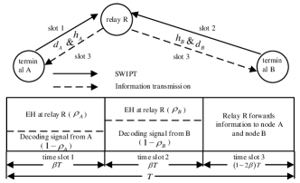
Figure 1: System model of the three-step two-way DF relay network.

As shown in Fig. 1, we consider a three-terminal two-way DF relay network, where terminal A communicates with terminal B via an energy-constrained relay R. Each terminal has a single antenna and operates in the half-duplex mode. We assume that no direct link exists between A and B due to severe path loss and shadowing [21, 22, 23, 24]. Channels are assumed to be reciprocal and quasi-static, and subject to path-loss Rayleigh fading. Let $h_{A}(h_{B})$ denote the channel coefficient between $A(B)$ and $R$, and ${d_{A}}({d_{B}})$ be the Euclidean distance between $A(B)$ and $R$. According to [30, 31], the path loss model is given by $\frac{{{G_{i}}{G_{R}}{\lambda^{2}}}}{{{{\left({4\pi{d_{0}}}\right)}^{2}}}}\times{\left({\frac{{{d_{0}}}}{d_{i}}}\right)^{\alpha}}\times|h_{i}|^{2}$ ($i=A\;\rm{or}\;B$), where $G_{i}$ is the antenna gain at terminal $i$, $G_{R}$ is the antenna gain at the relay, $\lambda$ is the carrier wavelength, $d_{0}$ is the close-in reference distance given from a measurement close to the transmitter and $\alpha$ is the path loss exponent. Further, the path loss model can be rewritten as $\Lambda_{i}{\left|h_{i}\right|^{2}}{d_{i}^{-\alpha}}$ ($i=A\;\rm{or}\;B$), where $\Lambda_{i}=\frac{{{G_{i}}{G_{R}}{\lambda^{2}}d_{0}^{\alpha-2}}}{{{{\left({4\pi}\right)}^{2}}}}$ is a fixed constant for a given scenario.

Here, we assume that the instantaneous channel coefficients between the two source terminals and the relay are available. Specifically, each source terminal needs to know the instantaneous channel coefficient between the source and the relay. The instantaneous channel coefficient is used to perform successive interference cancellation (SIC) at the source terminal. The relay needs to know the instantaneous channel coefficients between the two source terminals and the relay since the PS ratio for each link is determined by its instantaneous channel coefficient. Note that these instantaneous channel coefficients can be obtained before data transmission in each transmission block. Inspired by [32], we clarify how to obtain these instantaneous channel coefficients as follows. In the investigated system, terminal $A$ broadcasts a ready-to-send (RTS) message before information transmission. After receiving the RTS message, terminal $B$ replies with a clear-to-send (CTS) message. By overhearing the RTS and CTS messages, relay $R$ can estimate the channel coefficients of both $A$-$R$ and $B$-$R$ channels. Since all the channels are assumed to be reciprocal, the channel coefficients of both $R$-$A$ and $R$-$B$ channels can be obtained. Terminals $A$ and $B$ are informed of the corresponding channel coefficients through the feedbacks from the relay.

Let $T$ denote the total transmission block, which is sub-divided into three time slots. During the first and second time slots with $\beta T$ and $\beta\in(0,0.5)$, $A$ and $B$ transmit their normalized signal $s_{A}$ and $s_{B}$ to $R$ using equal power $P$, respectively. The received signal from $i$ ($i=A\;\rm{or}\;B$) at $R$ is given by

$${y_{iR}}={h_{i}}\sqrt{{P}\Lambda_{i}d_{i}^{-\alpha}}{s_{i}}+{n_{iR}},$$ (1)

where $\mathbb{E}\left\{{{{\left|s_{i}\right|}^{2}}}\right\}=1$ and ${n_{iR}}\sim{\rm{{\cal C}{\cal N}}}\left({0,\sigma_{iR}^{2}}\right)$ is the additive white Gaussian noise (AWGN).

After receiving signal from $i$ ($i=A\;\rm{or}\;B$), $R$ splits it into two parts: $\sqrt{\rho_{i}}{y_{iR}}$ used for energy harvesting (EH) and $\sqrt{1-\rho_{i}}{y_{iR}}$ used for information processing. For the energy harvesting, the total harvested energy during first two slots is

$$E_{\rm{total}}=\beta T\eta P\left({{{\rho_{A}}|{h_{A}}{|^{2}}\Lambda_{A}d_{A}^{-\alpha}}+{{\rho_{B}}|{h_{B}}{|^{2}}\Lambda_{B}d_{B}^{-\alpha}}}\right),$$ (2)

where $\eta$ is the energy conversion efficiency. For the information processing, the received SNR for decoding $s_{i}$ ($i=A\;\rm{or}\;B$) at the relay is

$${\gamma_{iR}}=\frac{{{P}|{h_{i}}{|^{2}}\Lambda_{i}\left({1-{\rho_{i}}}\right)}}{{d_{i}^{\alpha}\sigma_{iR}^{2}}}.$$ (3)

In the remaining part with $(1-2\beta)T$, $R$ combines the decoded signals $\widetilde{s}_{A}$ and $\widetilde{s}_{B}$ with a power allocation ratio $\theta\in(0,1)$ as $s_{R}=\frac{\theta\widetilde{s}_{A}+(1-\theta)\widetilde{s}_{B}}{\sqrt{\theta^{2}+(1-\theta)^{2}}}$. Note that the value of $\theta$ decides how the relay combines the decoded signals, $\widetilde{s}_{A}$ and $\widetilde{s}_{B}$.

Then $R$ broadcasts $s_{R}$ to both $A$ and $B$ with the harvested energy $E_{\rm{total}}$ and the received signal at $i$ ($i=A\;\rm{or}\;B$) is given by

$${y_{Ri}} ={h_{i}}\sqrt{{P_{R}}\Lambda_{i}d_{i}^{-\alpha}}{s_{R}}+{n_{Ri}},$$ (4)

where ${P_{R}}=\frac{{{E_{\rm{total}}}}}{{\left({1-2\beta}\right)T}}$ is the transmit power at $R$ and ${n_{Ri}}=\widetilde{n}_{Ri}\sim{\rm{{\cal C}{\cal N}}}\left({0,\sigma_{Ri}^{2}}\right)$ is the AWGN at $i$. For analytical simplicity, we assume $\sigma_{AR}^{2}=\sigma_{BR}^{2}=\sigma_{RA}^{2}=\sigma_{RB}^{2}={\sigma^{2}}$ [24].

After using SIC at $i$ ($i=A\;\rm{or}\;B$), the end-to-end SNR from $R$ to $i$ is given by

$${\gamma_{Ri}} ={X_{i}}\left({{\rho_{i}}|{h_{i}}{|^{4}}\Lambda_{i}d_{i}^{-\alpha}{\rm{+}}{\rho_{\bar{i}}}|{h_{\bar{i}}}{|^{2}}|{h_{i}}{|^{2}}\Lambda_{\bar{i}}d_{\bar{i}}^{-\alpha}}\right),$$ (5)

where ${X_{i}}=\left\{{\begin{array}[]{*{20}{c}}{\frac{{\beta\eta P\Lambda_{A}d_{A}^{-\alpha}{{\left({1-\theta}\right)}^{2}}}}{{\left({1-2\beta}\right){\sigma^{2}}\left[{{\theta^{2}}+{{\left({1-\theta}\right)}^{2}}}\right]}},\;{\rm{if}}\;i=A}\\ {\frac{{\beta\eta P\Lambda_{B}d_{B}^{-\alpha}{\theta^{2}}}}{{\left({1-2\beta}\right){\sigma^{2}}\left[{{\theta^{2}}+{{\left({1-\theta}\right)}^{2}}}\right]}},\;{\rm{if}}\;i=B}\end{array}}\right.$; if $i=A$, $\bar{i}=B$; if $i=B$, $\bar{i}=A$.

III Outage Analysis for Dynamic PS Scheme

In this section, we first propose a dynamic PS scheme to minimize the system outage probability, where the PS ratio for each terminal-relay link is adjusted based on its instantaneous CSI. Specifically, we obtain the optimal PS ratios in closed forms. Then, we derive the analytical expression for the optimal system outage probability with respect to the optimal PS ratios. Further, the corresponding outage capacity can also be obtained.

III-A Dynamic PS Scheme

Let $P_{\rm{out}}^{s}$ be the overall system outage probability. According to [14, 29], the system outage probability should jointly consider two E2E outage events and can be defined as the probability that any of the four link data rates is less than the data rate requirement. Thus, for a predefined SNR threshold ${\gamma_{\rm{th}}}$, $P_{\rm{out}}^{s}$ is given by

$$P_{\rm{out}}^{s}=1-P_{\rm{success}}^{s}$$

$$=1-\mathbb{P}\left({{\gamma_{AR}}\geq\gamma_{\rm{th}}},{{\gamma_{BR}}\geq\gamma_{\rm{th}}},{{\gamma_{RA}}\geq\gamma_{\rm{th}}},{{\gamma_{RB}}\geq\gamma_{\rm{th}}}\right),$$ (6)

where $P_{\rm{success}}^{s}$ is the probability that all the four transmissions are successful and $\mathbb{P}\left(\cdot\right)$ denotes the probability.

It is obvious that $P_{\rm{out}}^{s}$ is always equal to 1 for the cases with $\gamma_{AR}<\gamma_{\rm{th}}$ or $\gamma_{BR}<\gamma_{\rm{th}}$ since the relay can not decode the received signals successfully in such cases. Thus, in order to achieve the minimum system outage probability, both $\gamma_{AR}\geq\gamma_{\rm{th}}$ and $\gamma_{BR}\geq\gamma_{\rm{th}}$ should be satisfied. For the case with $\gamma_{AR}\geq\gamma_{\rm{th}}$ and $\gamma_{BR}\geq\gamma_{\rm{th}}$, the values of $\gamma_{RA}$ and $\gamma_{RB}$ decide whether the outage event happens or not for each transmission block, i.e., the lowest system outage probability can be obtained if we optimize $\rho_{A}$ and $\rho_{B}$ to maximize the value of $\min\left({{\gamma_{RA}},{\gamma_{RB}}}\right)$ for each transmission block. Therefore, minimizing the system outage probability is equivalent to maximizing the minimum SNR between $\gamma_{RA}$ and $\gamma_{RB}$ as

$$\begin{array}[]{*{20}{l}}{\mathbf{P1}:\mathop{{\rm{max}}}\limits_{({\rho_{A}},{\rho_{B}})}\;\;\min\left({{\gamma_{RA}},{\gamma_{RB}}}\right)}\\ \begin{array}[]{l}{\rm{s}}.{\rm{t}}.\;:\;{\gamma_{AR}}\geq{\gamma_{{\rm{th}}}};\\ \;\;\;\;\;\;\;\;\;\;{\gamma_{BR}}\geq{\gamma_{{\rm{th}}}}.\end{array}\end{array}$$ (11)

Based on ${{\gamma_{AR}}\geq\gamma_{\rm{th}}}$ and ${{\gamma_{BR}}\geq\gamma_{\rm{th}}}$, we have ${\rho_{i}}\leq 1-\frac{{{\gamma_{\rm{th}}}d_{i}^{\alpha}{\sigma^{2}}}}{{P\Lambda_{i}{{\left|{{h_{i}}}\right|}^{2}}}}$, where $i\in\left\{{A,B}\right\}$. Thus, the optimization problem $\mathbf{P1}$ can be further rewritten as

$$\begin{array}[]{*{20}{l}}{\mathbf{P2}:\mathop{{\rm{max}}}\limits_{({\rho_{A}},{\rho_{B}})}\;\;\min\left({\gamma_{RA}},{\gamma_{RB}}\right)}\\ {{\rm{s.t.}}\;:\;0\leq{\rho_{i}}\leq\max\left\{1-\frac{{{\gamma_{\rm{th}}}d_{i}^{\alpha}{\sigma^{2}}}}{{P\Lambda_{i}{{\left|{{h_{i}}}\right|}^{2}}}},0\right\},i\in\left\{{A,B}\right\}}.\!\!\!\end{array}$$ (14)

From (5), it is readily seen that ${\gamma_{RA}}\geq{\gamma_{RB}}$ holds for the case with $|{h_{A}}{|^{2}}\Lambda_{A}d_{A}^{-\alpha}{\left({1-\theta}\right)^{2}}\geq|{h_{B}}{|^{2}}\Lambda_{B}d_{B}^{-\alpha}{\theta^{2}}$ and that ${\gamma_{RA}}<{\gamma_{RB}}$ is satisfied for the case with $|{h_{A}}{|^{2}}\Lambda_{A}d_{A}^{-\alpha}{\left({1-\theta}\right)^{2}}<|{h_{B}}{|^{2}}\Lambda_{B}d_{B}^{-\alpha}{\theta^{2}}$. Since both ${\gamma_{RA}}$ and ${\gamma_{RB}}$ increase with the increase of ${\rho_{A}}$ and ${\rho_{B}}$, the optimal solution to $\mathbf{P2}$ can be obtained when $\rho_{A}=\max\left\{{1-\frac{{\gamma_{\rm{th}}d_{A}^{\alpha}{\sigma^{2}}}}{{P\Lambda_{A}{{\left|{{h_{A}}}\right|}^{2}}}},0}\right\}$ and $\rho_{B}=\max\left\{{1-\frac{{\gamma_{\rm{th}}d_{B}^{\alpha}{\sigma^{2}}}}{{P\Lambda_{B}{{\left|{{h_{B}}}\right|}^{2}}}},0}\right\}$. Thus, the optimal dynamic PS ratio $\rho^{\ast}_{i},i\in\left\{{A,B}\right\}$ is given by

$$\rho_{i}^{*}=\max\left\{{1-\frac{{\varpi Z_{i}}}{{{{\left|{{h_{i}}}\right|}^{2}}}},0}\right\},$$ (15)

where $\varpi=\frac{{{\gamma_{\rm{th}}}{\sigma^{2}}}}{P}$ and $Z_{i}=\frac{d_{i}^{\alpha}}{\Lambda_{i}}$.

III-B System Outage Probability

Substituting the optimal PS ratios in (15) into (III-A), $P_{\rm{out}}^{s}$ can be expressed as

$$P_{\rm{out}}^{s}=1-\mathbb{P}\bigg{(}|{h_{A}}{|^{2}}\geq\Phi_{1},|{h_{B}}{|^{2}}\geq\Phi_{2}\bigg{)},$$ (16)

where $\Phi_{1}=\max\left(\varpi Z_{A}{,\frac{{{\gamma_{\rm{th}}}Z_{A}}}{{{X_{B}}|{h_{B}}{|^{2}}}}+2\varpi Z_{A}-|{h_{B}}{|^{2}}Z_{B}^{-1}Z_{A}}\right)$ and $\Phi_{2}=\max\left(\varpi Z_{B}{,\frac{{{\gamma_{\rm{th}}}Z_{B}}}{{{X_{A}}|{h_{A}}{|^{2}}}}+2\varpi Z_{B}-|{h_{A}}{|^{2}}Z_{A}^{-1}Z_{B}}\right)$. Based on the values of $\Phi_{1}$ and $\Phi_{2}$, $P_{\rm{out}}^{s}$ can be rewritten as

$$P_{\rm{out}}^{s}=1-(P^{s}_{\rm{case1}}+P^{s}_{\rm{case2}}+P^{s}_{\rm{case3}}+P^{s}_{\rm{case4}}),$$ (17)

where $P^{s}_{\rm{case1}}=\mathbb{P}\left(|{h_{A}}{|^{2}}\geq\Phi_{1},|{h_{B}}{|^{2}}\geq\Phi_{2}\right)$ with $\Phi_{1}=\frac{{{\gamma_{\rm{th}}}Z_{A}}}{{{X_{B}}|{h_{B}}{|^{2}}}}+2\varpi Z_{A}-|{h_{B}}{|^{2}}Z_{B}^{-1}Z_{A}$ and $\Phi_{2}=\varpi Z_{B}$; $P^{s}_{\rm{case2}}=\mathbb{P}\left(|{h_{A}}{|^{2}}\geq\Phi_{1},|{h_{B}}{|^{2}}\geq\Phi_{2}\right)$ with $\Phi_{1}=\varpi Z_{A}$ and $\Phi_{2}=\frac{{{\gamma_{\rm{th}}}Z_{B}}}{{{X_{A}}|{h_{A}}{|^{2}}}}+2\varpi Z_{B}-|{h_{A}}{|^{2}}Z_{A}^{-1}Z_{B}$; $P^{s}_{\rm{case3}}=\mathbb{P}\left(|{h_{A}}{|^{2}}\geq\Phi_{1},|{h_{B}}{|^{2}}\geq\Phi_{2}\right)$ with $\Phi_{1}=\varpi Z_{A}$ and $\Phi_{2}=\varpi Z_{B}$; and $P^{s}_{\rm{case4}}=\mathbb{P}\left(|{h_{A}}{|^{2}}\geq\Phi_{1},|{h_{B}}{|^{2}}\geq\Phi_{2}\right)$ with $\Phi_{1}=\frac{{{\gamma_{\rm{th}}}Z_{A}}}{{{X_{B}}|{h_{B}}{|^{2}}}}+2\varpi Z_{A}-|{h_{B}}{|^{2}}Z_{B}^{-1}Z_{A}$ and $\Phi_{2}=\frac{{{\gamma_{\rm{th}}}Z_{B}}}{{{X_{A}}|{h_{A}}{|^{2}}}}+2\varpi Z_{B}-|{h_{A}}{|^{2}}Z_{A}^{-1}Z_{B}$.

Then, the rest of this section is devoted to deriving $P^{s}_{\rm{case1}}$, $P^{s}_{\rm{case2}}$, $P^{s}_{\rm{case3}}$ and $P^{s}_{\rm{case4}}$.

III-B1 Derivation of $P^{s}_{\rm{case1}}$

Based on the conditions $\Phi_{1}=\frac{{{\gamma_{\rm{th}}}Z_{A}}}{{{X_{B}}|{h_{B}}{|^{2}}}}+2\varpi Z_{A}-|{h_{B}}{|^{2}}Z_{B}^{-1}Z_{A}$ and $\Phi_{2}=\varpi Z_{B}$, the following two equations should be satisfied:

$$\left\{{\begin{array}[]{*{20}{c}}{\frac{{{\gamma_{\rm{th}}}}}{{{X_{B}}}}+\varpi|{h_{B}}{|^{2}}-|{h_{B}}{|^{4}}Z_{B}^{-1}\geq 0},\\ {\frac{{{\gamma_{\rm{th}}}}}{{{X_{A}}}}+\varpi|{h_{A}}{|^{2}}-|{h_{A}}{|^{4}}Z_{A}^{-1}<0}.\end{array}}\right.$$ (20)

Combining $|{h_{A}}{|^{2}}\geq 0$ and $|{h_{B}}{|^{2}}\geq 0$, the solution to (20) is $0\leq|{h_{B}}{|^{2}}\leq\Delta_{B}$ and $|{h_{A}}{|^{2}}>\Delta_{A}$, where $\Delta_{B}=\frac{{\varpi+\sqrt{{\varpi^{2}}+4{\gamma_{{\rm{th}}}}Z_{B}^{-1}/{X_{B}}}}}{2}{Z_{B}}$ and $\Delta_{A}=\frac{{\varpi+\sqrt{{\varpi^{2}}+4{\gamma_{{\rm{th}}}}Z_{A}^{-1}/{X_{A}}}}}{2}{Z_{A}}$. Since $\Delta_{B}>\varpi Z_{B}$ and $\Delta_{A}>\varpi Z_{A}$, $P^{s}_{\rm{case1}}$ is given by

$$P^{s}_{\rm{case1}} =\mathbb{P}\bigg{(}|{h_{A}}{|^{2}}\geq\phi_{A}\left({|{h_{B}}{|^{2}}}\right),\varpi Z_{B}\leq|{h_{B}}{|^{2}}\leq{\Delta_{B}}\bigg{)}$$

$$\overset{\text{(a)}}{=}\frac{1}{{{\lambda_{B}}}}\int_{\varpi Z_{B}}^{{\Delta_{B}}}{\exp\left({-\frac{{\phi_{A}\left(x\right)}}{{{\lambda_{A}}}}-\frac{x}{{{\lambda_{B}}}}}\right)}dx,$$ (21)

where $\phi_{A}\left({|{h_{B}}{|^{2}}}\right)=\max\left({\frac{{{\gamma_{{\rm{th}}}}Z_{A}}}{{{X_{B}}{|{h_{B}}{|^{2}}}}}+2\varpi Z_{A}-\frac{{|{h_{B}}{|^{2}}}Z_{A}}{Z_{B}},{\Delta_{A}}}\right)$ and step (a) holds from $x={{{\left|{{h_{B}}}\right|}^{2}}}$ and ${\left|{{h_{i}}}\right|^{2}}\sim\exp\left({\frac{1}{{\lambda_{i}}}}\right)$ for $i\in\left\{{A,B}\right\}$.

Since there is no closed-form expression for the integral $\int_{{s_{1}}}^{{s_{2}}}{\exp({z_{1}}x+\frac{{{z_{2}}}}{x})}dx$ with any value of $z_{1}$ and $z_{2}\neq 0$, here we employ Gaussian-Chebyshev quadrature [9, 34] to achieve an approximation for $P^{s}_{\rm{case1}}$ as

$$P^{s}_{\rm{case1}}\approx$$

$$\frac{{\pi({\Delta_{B}}-\varpi Z_{B})}}{{2M{\lambda_{B}}}}\sum\limits_{m=1}^{M}\sqrt{1-\nu_{m}^{2}}\exp\left({-\frac{{\phi_{A}\left({\kappa_{m}^{B}}\right)}}{{{\lambda_{A}}}}-\frac{{\kappa_{m}^{B}}}{{{\lambda_{B}}}}}\right),$$ (22)

where $M$ is a parameter that determines the tradeoff between complexity and accuracy , ${\nu_{m}}=\cos\frac{{2m-1}}{{2M}}\pi$, and $\kappa_{m}^{i}=\frac{{({\Delta_{i}}-\varpi Z_{i})}}{2}{\nu_{m}}+\frac{{(\varpi Z_{i}+{\Delta_{i}})}}{2}$ for $i\in\left\{{A,B}\right\}$.

III-B2 Derivation of $P^{s}_{\rm{case2}}$

Based on $\Phi_{1}=\varpi d_{A}^{\alpha}$ and $\Phi_{2}=\frac{{{\gamma_{\rm{th}}}Z_{B}}}{{{X_{A}}|{h_{A}}{|^{2}}}}+2\varpi Z_{B}-|{h_{A}}{|^{2}}Z_{A}^{-1}Z_{B}$, we have $|{h_{B}}{|^{2}}>{\Delta_{B}}$ and $0\leq|{h_{A}}{|^{2}}\leq{\Delta_{A}}$. Then $P^{s}_{\rm{case2}}$ can be calculated as

$$P^{s}_{\rm{case2}}=\mathbb{P}\bigg{(}|{h_{B}}{|^{2}}\geq{\phi_{B}}\left({|{h_{A}}{|^{2}}}\right),\varpi Z_{A}\leq|{h_{A}}{|^{2}}\leq{\Delta_{A}}\bigg{)}\approx$$

$$\frac{{\pi({\Delta_{A}}-\varpi Z_{A})}}{{2M{\lambda_{A}}}}\sum\limits_{m=1}^{M}{\sqrt{1-\nu_{m}^{2}}}\exp\left({-\frac{{{\phi_{B}}\left({\kappa_{m}^{A}}\right)}}{{{\lambda_{B}}}}-\frac{{\kappa_{m}^{A}}}{{{\lambda_{A}}}}}\right),$$ (23)

where ${\phi_{B}}\left({|{h_{A}}{|^{2}}}\right)=\max\left({\frac{{{\gamma_{{\rm{th}}}}Z_{B}}}{{{X_{A}}|{h_{A}}{|^{2}}}}+2\varpi Z_{B}-\frac{{|{h_{A}}{|^{2}}Z_{B}}}{{Z_{A}}},{\Delta_{B}}}\right)$.

III-B3 Derivation of $P^{s}_{\rm{case3}}$

Based on $|{h_{A}}{|^{2}}\geq\Phi_{1}=\varpi Z_{A}$ and $|{h_{B}}{|^{2}}\geq\Phi_{2}=\varpi Z_{B}$, the ranges of $|{h_{A}}{|^{2}}$ and $|{h_{B}}{|^{2}}$ can be given by $|{h_{B}}{|^{2}}>{\Delta_{B}}$ and $|{h_{A}}{|^{2}}>{\Delta_{A}}$, respectively. Thus $P^{s}_{\rm{case3}}$ is given by

$$P^{s}_{\rm{case3}} =\mathbb{P}\bigg{(}|{h_{A}}{|^{2}}>{\Delta_{A}},|{h_{B}}{|^{2}}>{\Delta_{B}}\bigg{)}$$

$$=\exp\left({-\frac{{{\Delta_{A}}}}{{{\lambda_{A}}}}-\frac{{{\Delta_{B}}}}{{{\lambda_{B}}}}}\right).$$ (24)

III-B4 Derivation of $P^{s}_{\rm{case4}}$

Based on $\Phi_{1}=\frac{{{\gamma_{\rm{th}}}Z_{A}}}{{{X_{B}}|{h_{B}}{|^{2}}}}+2\varpi Z_{A}-|{h_{B}}{|^{2}}Z_{B}^{-1}Z_{A}$ and $\Phi_{2}=\frac{{{\gamma_{\rm{th}}}Z_{B}}}{{{X_{A}}|{h_{A}}{|^{2}}}}+2\varpi Z_{B}-|{h_{A}}{|^{2}}Z_{A}^{-1}Z_{B}$, the ranges of $|{h_{A}}{|^{2}}$ and $|{h_{B}}{|^{2}}$ can be determined by $0\leq|{h_{B}}{|^{2}}\leq\Delta_{B}$ and $0\leq|{h_{A}}{|^{2}}\leq\Delta_{A}$. Thus $P^{s}_{\rm{case4}}$ can be computed as

$$P^{s}_{\rm{case4}}=\mathbb{P}\left(\Phi_{1}\leq|{h_{A}}{|^{2}}\leq{\Delta_{A}},\Phi_{2}\leq|{h_{B}}{|^{2}}\leq{\Delta_{B}}\right).$$ (25)

Clearly, $\Phi_{1}$ and $\Phi_{2}$ are highly correlated, which is the main difficulty in deriving $P^{s}_{\rm{case4}}$. Here, we first determine the integral region that determines the probability $P^{s}_{\rm{case4}}$. Then we obtain the value of $P^{s}_{\rm{case4}}$ by calculating the integral value over that region.

Let $|{h_{A}}{|^{2}}=x$ and $|{h_{B}}{|^{2}}=y$. From the expression of $P^{s}_{\rm{case4}}$ in (25), the integral region of $P^{s}_{\rm{case4}}$ is bounded by 4 lines, which are $y=\frac{{{\gamma_{{\rm{th}}}}Z_{B}}}{{{X_{A}}x}}+2\varpi Z_{B}-xZ_{A}^{-1}Z_{B}$ (Line 1), $x=\frac{{{\gamma_{{\rm{th}}}}Z_{A}}}{{{X_{B}}y}}+2\varpi Z_{A}-yZ_{B}^{-1}Z_{A}$ (Line 2), $x={\Delta_{A}}$ (Line 3) and $y={\Delta_{B}}$ (Line 4). Let the intersection points between Line 1 and Line 3 as well as between Line 1 and Line 4 be $(x_{1},q_{1})$ or $(x_{\Delta},y_{1})$, respectively.

For $(x_{1},q_{1})$, the following two equations should be satisfied:

$$\left\{{\begin{array}[]{*{20}{c}}{q_{1}=\frac{{{\gamma_{{\rm{th}}}}Z_{B}}}{{{X_{A}}x_{1}}}+2\varpi Z_{B}-x_{1}Z_{A}^{-1}Z_{B}},\\ {x_{1}={\Delta_{A}}}.\end{array}}\right.$$ (28)

Substituting $x_{1}={\Delta_{A}}$ into the first equation of (28), we have $q_{1}=\frac{{{\gamma_{{\rm{th}}}}Z_{B}}}{{{X_{A}}{{\Delta_{A}}}}}+2\varpi Z_{B}-{{\Delta_{A}}}Z_{A}^{-1}Z_{B}$ and $(x_{1},q_{1})$ is given by $\left({\Delta_{A}},\frac{{{\gamma_{{\rm{th}}}}Z_{B}}}{{{X_{A}}{{\Delta_{A}}}}}+2\varpi Z_{B}-{{\Delta_{A}}}Z_{A}^{-1}Z_{B}\right)$.

Similarly, for $(x_{\Delta},y_{1})$, we have

$$\left\{{\begin{array}[]{*{20}{c}}{y_{1}=\frac{{{\gamma_{{\rm{th}}}}Z_{B}}}{{{X_{A}}x_{\Delta}}}+2\varpi Z_{B}-x_{\Delta}Z_{A}^{-1}Z_{B}},\\ {y_{1}={\Delta_{B}}}.\end{array}}\right..$$ (31)

Further, (31) can be rewritten as

$$\frac{{{\gamma_{{\rm{th}}}}Z_{B}}}{{{X_{A}}}}+\left(2\varpi Z_{B}-{\Delta_{B}}\right)x_{\Delta}-x_{\Delta}^{2}Z_{A}^{-1}Z_{B}=0.$$ (32)

Since $x_{\Delta}\geq 0$, $x_{\Delta}$ is given by $\frac{{2\varpi{Z_{B}}-{\Delta_{B}}+\sqrt{{{\left({2\varpi{Z_{B}}-{\Delta_{B}}}\right)}^{2}}+4{\gamma_{{\rm{th}}}}Z_{A}^{-1}Z_{B}^{2}/{X_{A}}}}}{{2{Z_{B}}Z_{A}^{-1}}}$. Thus, $(x_{\Delta},y_{1})$ is given by $\left(\frac{{2\varpi{Z_{B}}-{\Delta_{B}}+\sqrt{{{\left({2\varpi{Z_{B}}-{\Delta_{B}}}\right)}^{2}}+4{\gamma_{{\rm{th}}}}Z_{A}^{-1}Z_{B}^{2}/{X_{A}}}}}{{2{Z_{B}}Z_{A}^{-1}}},{\Delta_{B}}\right)$.

Similarly, the intersection points between Line 2 and Line 3 as well as between Line 1 and Line 4 are $(x_{1},y_{\Delta})$ and $(q_{2},y_{1})$ respectively, where $y_{\Delta}=\frac{{2\varpi{Z_{A}}-{\Delta_{A}}+\sqrt{{{\left({2\varpi{Z_{A}}-{\Delta_{A}}}\right)}^{2}}+4{\gamma_{{\rm{th}}}}Z_{B}^{-1}Z_{A}^{2}/{X_{B}}}}}{{2{Z_{A}}Z_{B}^{-1}}}$ and $q_{2}=\frac{{{\gamma_{{\rm{th}}}}Z_{A}}}{{{X_{B}}{{\Delta_{B}}}}}+2\varpi Z_{A}-{{\Delta_{B}}}Z_{B}^{-1}Z_{A}$.

Let $(x_{+},y_{+})$ denote the intersection point between Line 1 and Line 2. Then $(x_{+},y_{+})$ should satisfy

$$\left\{\begin{array}[]{l}x_{+}=\frac{{{C_{A}}}}{y_{+}}+{E_{A}}-{D_{A}}y_{+},\\ y_{+}=\frac{{{C_{B}}}}{x_{+}}+{E_{B}}-{D_{B}}x_{+},\end{array}\right.$$ (35)

where ${C_{i}}=\frac{{{\gamma_{{\rm{th}}}}Z_{i}}}{{{X_{\bar{i}}}}}$, ${D_{i}}=Z_{\bar{i}}^{-1}Z_{i}$ and ${E_{i}}=2\varpi Z_{i}$.

Further, (35) can be transformed as

$$\left({{C_{A}}+{C_{B}}}\right){x_{+}^{2}}-{C_{B}}{E_{A}}x_{+}-{D_{A}}C_{B}^{2}=0.$$ (36)

Since $x_{+}>0$, the solution to (36) is given by $x_{+}=\frac{{{C_{B}}{E_{A}}+\sqrt{C_{B}^{2}E_{A}^{2}+4{D_{A}}C_{B}^{2}\left({{C_{A}}+{C_{B}}}\right)}}}{{2\left({{C_{A}}+{C_{B}}}\right)}}$. Then the corresponding value of $y_{+}$ is given by $\frac{{{C_{B}}}}{x_{+}}+{E_{B}}-{D_{B}}x_{+}$.

Based on the positions of all the intersections, there can be three scenarios for $P^{s}_{\rm{case4}}$, discussed as follows.

Scenario 1: When $\max\left({{q_{2}},{x_{\Delta}}}\right)\geq{x_{1}}$ or $\max\left({{q_{1}},{y_{\Delta}}}\right)\geq{y_{1}}$, the integral of region for $P^{s}_{\rm{case4}}$ is $0$. Thus, we have $P^{s}_{\rm{case4}}=0$.

Scenario 2: When $\max\left({{q_{2}},{x_{\Delta}}}\right)<{x_{1}}$, $\max\left({{q_{1}},{y_{\Delta}}}\right)<{y_{1}}$, and $x_{+}\leq\max\left({{q_{2}},{x_{\Delta}}}\right)$ (or $x_{+}\geq x_{1}$) hold, the integral of region for $P^{s}_{\rm{case4}}$ is bounded by three lines, which are Line 3, Line 4, and Line 1 (or Line 2).

For the case with $y_{\Delta}\geq q_{1}$, the integral of region is bounded by Line 2, Line 3, and Line 4. Then $P^{s}_{\rm{case4}}$ is calculated as

$$P^{s}_{\rm{case4}}=\mathbb{P}\left(\Phi_{1}\leq|{h_{A}}{|^{2}}\leq x_{1},y_{\Delta}\leq|{h_{B}}{|^{2}}\leq y_{1}\right)$$

$$=\frac{1}{{{\lambda_{B}}}}\exp\left({-\frac{{{E_{A}}}}{{{\lambda_{A}}}}}\right)\int_{{y_{\Delta}}}^{{y_{1}}}{\exp\left({\vartheta_{A}}\left(y\right)\right)}dy-{f_{A}}({x_{1}},{y_{\Delta}},{y_{1}})$$

$$\overset{\text{(b)}}{\approx}\frac{{\pi({y_{1}}-{y_{\Delta}})\exp\left({-\frac{{{E_{A}}}}{{{\lambda_{A}}}}}\right)}}{{2M{\lambda_{B}}}}\sum\limits_{m=1}^{M}{\sqrt{1-\nu_{m}^{2}}}\exp\left({{\vartheta_{A}}\left({\kappa_{m}^{(1)}}\right)}\right)$$

$$-{f_{A}}({x_{1}},{y_{\Delta}},{y_{1}}),$$ (37)

where step (b) holds by using Gaussian-Chebyshev quadrature, ${\vartheta_{i}}\left({\kappa_{m}^{(1)}}\right)=-\frac{{{C_{i}}}}{{{\lambda_{i}}\kappa_{m}^{(1)}}}+\left({\frac{{{D_{i}}}}{{{\lambda_{i}}}}-\frac{1}{{{\lambda_{\bar{i}}}}}}\right)\kappa_{m}^{(1)}$, ${f_{i}}({x_{1}},{y_{\Delta}},{y_{1}})=\exp\left({-\frac{{{x_{1}}}}{{{\lambda_{i}}}}}\right)\left({\exp\left({-\frac{{{y_{\Delta}}}}{{{\lambda_{\bar{i}}}}}}\right)-\exp\left({-\frac{{{y_{1}}}}{{{\lambda_{\bar{i}}}}}}\right)}\right)$ and $\kappa_{m}^{(1)}=\frac{{({y_{1}}-{y_{\Delta}})}}{2}{\nu_{m}}+\frac{{({y_{1}}+{y_{\Delta}})}}{2}$.

Likewise, for the case with $y_{\Delta}<q_{1}$, the integral of region is bounded by Line 1, Line 3, and Line 4 and $P^{s}_{\rm{case4}}$ is given by

$$P^{s}_{\rm{case4}}=\mathbb{P}\left(\Phi_{2}\leq|{h_{B}}{|^{2}}\leq y_{1},x_{\Delta}\leq|{h_{A}}{|^{2}}\leq x_{1}\right)$$

$$\approx\frac{{\pi({x_{1}}-{x_{\Delta}})\exp\left({-\frac{{{E_{B}}}}{{{\lambda_{B}}}}}\right)}}{{2M{\lambda_{A}}}}\sum\limits_{m=1}^{M}{\sqrt{1-\nu_{m}^{2}}}\exp\left({{\vartheta_{B}}\left({\kappa_{m}^{(2)}}\right)}\right)$$

$$-{f_{B}}({y_{1}},{x_{\Delta}},{x_{1}}),$$ (38)

where $\kappa_{m}^{(2)}=\frac{{({x_{1}}-{x_{\Delta}})}}{2}{\nu_{m}}+\frac{{({x_{1}}+{x_{\Delta}})}}{2}$.

Scenario 3: When $\max\left({{q_{2}},{x_{\Delta}}}\right)<{x_{1}}$, $\max\left({{q_{1}},{y_{\Delta}}}\right)<{y_{1}}$, and $\max\left({{q_{2}},{x_{\Delta}}}\right)<x_{+}<x_{1}$ are satisfied, the integral region is bounded by 4 lines.

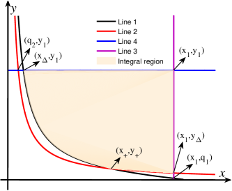
Figure 2: Integral region for Scenario 3 of $P^{s}_{\rm{case4}}$ with $y_{\Delta}\geq q_{1}$.

For $y_{\Delta}\geq q_{1}$, the lower bounds with $x\in[\max\left({{q_{2}},{x_{\Delta}}}\right),x_{+}]$ and $x\in[x_{+},x_{1}]$ are Line 1 and Line 2, respectively, as shown in Fig. 2. In this case, $P^{s}_{\rm{case4}}$ can be computed as

$$P^{s}_{\rm{case4}}=\mathbb{P}\left(\Phi_{2}\leq|{h_{B}}{|^{2}}\leq y_{1},x_{\Delta}\leq|{h_{A}}{|^{2}}\leq x_{+}\right)$$

$$+\mathbb{P}\left(\Phi_{1}\leq|{h_{A}}{|^{2}}\leq x_{1},y_{\Delta}\leq|{h_{B}}{|^{2}}\leq y_{+}\right)$$

$$+\mathbb{P}\left(y_{+}\leq|{h_{B}}{|^{2}}\leq y_{1},x_{+}\leq|{h_{A}}{|^{2}}\leq x_{1}\right)\approx$$

$$\frac{\pi}{{2M}}\!\!\sum\limits_{m=1}^{M}\!\!\!\!{\sqrt{1-\nu_{m}^{2}}}\!\!\!\!\sum\limits_{i=\left\{{A,B}\right\}}\!\!\!\!\!\!{\frac{{\Delta_{\max}^{i}-\Delta_{\min}^{i}}}{{{\lambda_{i}}}}\exp\left({{\vartheta_{\bar{i}}}\left({\kappa_{m}^{(i)}}\right)-\frac{{{E_{\bar{i}}}}}{{{\lambda_{\bar{i}}}}}}\right)}+$$

$$\Xi_{A}(x_{+},x_{1},y_{+},y_{1})\!-\!{f_{B}}({y_{1}},{x_{\Delta}},{x_{+}})\!-\!{f_{A}}({x_{1}},{y_{\Delta}},{y_{+}}),\!\!\!\!$$ (39)

where $\Delta_{\max}^{i}$ is determined by $\left\{{\begin{array}[]{*{20}{c}}{{x_{+}},{\rm{}}i=A}\\ {{y_{+}},{\rm{}}i=B}\end{array}}\right.$; $\Delta_{\min}^{i}$ is given by $\left\{{\begin{array}[]{*{20}{c}}{{x_{\Delta}},{\rm{}}i=A}\\ {{y_{\Delta}},{\rm{}}i=B}\end{array}}\right.$; $\kappa_{m}^{(i)}$ is given by $\frac{{(\Delta_{\max}^{i}-\Delta_{\min}^{i})}}{2}{\nu_{m}}+\frac{{(\Delta_{\max}^{i}+\Delta_{\min}^{i})}}{2}$; and $\Xi_{i}(x_{+},x_{1},y_{+},y_{1})=\left({\exp\left({-\frac{{{x_{+}}}}{{{\lambda_{i}}}}}\right)-\exp\left({-\frac{{{x_{1}}}}{{{\lambda_{i}}}}}\right)}\right)\left({\exp\left({-\frac{{{y_{+}}}}{{{\lambda_{\bar{i}}}}}}\right)-\exp\left({-\frac{{{y_{1}}}}{{{\lambda_{\bar{i}}}}}}\right)}\right)$.

For $y_{\Delta}<q_{1}$, the lower bounds with $x\in[\max\left({{q_{2}},{x_{\Delta}}}\right),x_{+}]$ and $x\in[x_{+},x_{1}]$ are Line 2 and Line 1, respectively. In this case, $P^{s}_{\rm{case4}}$ is given by

$$P^{s}_{\rm{case4}}\approx-{f_{B}}({y_{+}},{x_{+}},{x_{1}})-{f_{A}}({x_{1}},{y_{+}},{y_{1}})+$$

$$\frac{\pi}{{2M}}\!\!\sum\limits_{m=1}^{M}\!\!\!{\sqrt{1-\nu_{m}^{2}}}\!\!\!\!\sum\limits_{i=\left\{{A,B}\right\}}\!\!\!\!\!\!{\frac{{\omega_{\max}^{i}-\omega_{\min}^{i}}}{{{\lambda_{i}}}}\exp\left({{\vartheta_{\bar{i}}}\left({\kappa_{m}^{[i]}}\right)-\frac{{{E_{\bar{i}}}}}{{{\lambda_{\bar{i}}}}}}\right)},$$ (40)

where $\omega_{\max}^{i}$ is given by $\left\{{\begin{array}[]{*{20}{c}}{{x_{1}},{\rm{}}i=A}\\ {{y_{1}},{\rm{}}i=B}\end{array}}\right.$; $\omega_{\min}^{i}=\left\{{\begin{array}[]{*{20}{c}}{{x_{+}},{\rm{}}i=A}\\ {{y_{+}},{\rm{}}i=B}\end{array}}\right.$; and $\kappa_{m}^{[i]}$ is given by $\frac{{(\omega_{\max}^{i}-\omega_{\min}^{i})}}{2}{\nu_{m}}+\frac{{(\omega_{\max}^{i}+\omega_{\min}^{i})}}{2}$.

$$P_{\rm{out}}^{s}\approx 1-\exp\left({-\frac{{{\Delta_{A}}}}{{{\lambda_{A}}}}-\frac{{{\Delta_{B}}}}{{{\lambda_{B}}}}}\right)-\frac{\pi}{{2M}}\sum\limits_{m=1}^{M}{\sqrt{1-\nu_{m}^{2}}}\sum\limits_{i=\left\{{A,B}\right\}}{\frac{{{\Delta_{i}}-\varpi Z_{i}}}{{{\lambda_{i}}}}\exp\left({-\frac{{{\phi_{\bar{i}}}\left({\kappa_{m}^{i}}\right)}}{{{\lambda_{\bar{i}}}}}-\frac{{\kappa_{m}^{i}}}{{{\lambda_{i}}}}}\right)}-\Theta,$$ (41)

where

$$\Theta=\left\{{\begin{array}[]{*{20}{c}}{\!\!\!\!\!\!\!\!\!\!\!\!\!\!\!\!0,{\rm{\;Scenario\;1;}}}\\ \!\!\!\!\!\!\!\!\!\!\!\!\!\!\!\!\!\!\!\!\!\!\!\!\!\!\!\!\!\!\!\!\!\!\!\!\!\!\!\!\!\!\!{\frac{{\pi({y_{1}}-{y_{\Delta}})\exp\left({-\frac{{{E_{A}}}}{{{\lambda_{A}}}}}\right)}}{{2M{\lambda_{B}}}}\sum\limits_{m=1}^{M}{\sqrt{1-\nu_{m}^{2}}}\exp\left({{\vartheta_{A}}\left({\kappa_{m}^{(1)}}\right)}\right)-{f_{A}}({x_{1}},{y_{\Delta}},{y_{1}}),\;{\rm{Scenario\;2\;with\;}}{y_{\Delta}}\geq{q_{1}}};\\ \!\!\!\!\!\!\!\!\!\!\!\!\!\!\!\!\!\!\!\!\!\!\!\!\!\!\!\!\!\!\!\!\!\!\!\!\!\!\!\!\!\!\!\!\!{\frac{{\pi({x_{1}}-{x_{\Delta}})\exp\left({-\frac{{{E_{B}}}}{{{\lambda_{B}}}}}\right)}}{{2M{\lambda_{A}}}}\sum\limits_{m=1}^{M}{\sqrt{1-\nu_{m}^{2}}}\exp\left({{\vartheta_{B}}\left({\kappa_{m}^{(2)}}\right)}\right)-{f_{B}}({y_{1}},{x_{\Delta}},{x_{1}}),{\rm{\;Scenario\;2\;with\;}}{y_{\Delta}}<{q_{1}}};\\ \begin{array}[]{l}\!\!\!\!\!\!{\Xi_{A}}({x_{+}},{x_{1}},{y_{+}},{y_{1}})+\frac{\pi}{{2M}}\sum\limits_{m=1}^{M}{\sqrt{1-\nu_{m}^{2}}}\sum\limits_{i=\left\{{A,B}\right\}}{\frac{{\Delta_{\max}^{i}-\Delta_{\min}^{i}}}{{{\lambda_{i}}}}\exp\left({{\vartheta_{\bar{i}}}\left({\kappa_{m}^{(i)}}\right)-\frac{{{E_{\bar{i}}}}}{{{\lambda_{\bar{i}}}}}}\right)}-{f_{B}}({y_{1}},{x_{\Delta}},{x_{+}})-{f_{A}}({x_{1}},{y_{\Delta}},{y_{+}}),\\ \;\;\;\;\;\;\;\;\;\;\;\;\;\;\;\;\;\;\;\;\;\;\;\;\;\;\;\;\;\;\;\;\;\;\;\;\;\;\;\;\;\;\;\;\;\;\;\;\;\;\;\;\;\;\;\;\;\;\;\;\;\;\;\;\;\;\;\;\;\;\;\;\;\;\;\;\;\;\;\;\;\;\;\;\;\;\;\;\;\;\;\;\;\;\;\;\;\;\;\;\;\;\;\;\;\;\;\;\;\;\;\;\;\;\;\;\;\;\;\;\;\;\;\;\;\;\;\;\;\;\;\;\;\;\;\;\;\;\;\;{\rm{Scenario\;3\;with\;}}{y_{\Delta}}\geq{q_{1}};\\ \!\!\!\!\!\!\frac{\pi}{{2M}}\sum\limits_{m=1}^{M}{\sqrt{1-\nu_{m}^{2}}}\sum\limits_{i=\left\{{A,B}\right\}}{\frac{{\omega_{\max}^{i}-\omega_{\min}^{i}}}{{{\lambda_{i}}}}\exp\left({{\vartheta_{\bar{i}}}\left({\kappa_{m}^{[i]}}\right)-\frac{{{E_{\bar{i}}}}}{{{\lambda_{\bar{i}}}}}}\right)}-{f_{B}}\left({{y_{+}},{x_{+}},{x_{1}}}\right)-{f_{A}}\left({{x_{1}},{y_{+}},{y_{1}}}\right),{\rm{\;Scenario\;3\;with\;}}{y_{\Delta}}<{q_{1}}.{\rm{}}\end{array}\end{array}}\right..$$ (49)

Combining (17) with $P^{s}_{\rm{case1}}$, $P^{s}_{\rm{case2}}$, $P^{s}_{\rm{case3}}$ and $P^{s}_{\rm{case4}}$, the value of $P_{\rm{out}}^{s}$ can be determined in (41) at the top of next page.

Remark: The derived expression for system outage probability in (41) serves the following purposes. First, (41) can characterize the system outage probability of SWIPT enabled three-step two-way DF relay networks for the dynamic PS scheme with a small $M$ and certain accuracy instead of carrying out computer simulations. Second, we can obtain some insightful understandings on selecting proper system parameters based on the curves obtained by (41). Note that this approach has also adopted in many works, e.g., [11, 13, 24]. Third, based on the derived expression in (41), we can compute the system outage capacity and analyze the diversity gain for our investigated network, as shown in Section III.C and Section III.D.

III-C System Outage Capacity

Based on the analytical result of the system outage probability in (41), we can obtain the system outage capacity for the dynamic PS scheme, denoted by $\tau^{\rm{DPS}}$. Since both $A$ and $B$ transmit signals at the transmission rate $U=\log_{2}(1+\gamma_{\rm{th}})$, and the effective transmission time is given by the minimum of $\beta T$ and $(1-2\beta)T$, the system outage capacity $\tau^{\rm{DPS}}$ is given by

$$\tau^{\rm{DPS}}=(1-P_{\rm{out}}^{s})U\times\min\left(\beta T,(1-2\beta)T\right).$$ (50)

III-D Diversity Gain

According to [9, 15], the diversity gain of the investigated system under the dynamic PS scheme can be computed as

$$d=-\mathop{\lim}\limits_{{\rho_{0}}\to\infty}\frac{{\log\left(P_{\rm{out}}^{s}\right)}}{{\log\left({{\rho_{0}}}\right)}}$$

$$=\!-\!\mathop{\lim}\limits_{{\rho_{0}}\to\infty}\frac{{\log\left({1-P^{s}_{\rm{case1}}-P^{s}_{\rm{case2}}-P^{s}_{\rm{case3}}-P^{s}_{\rm{case4}}}\right)}}{{\log\left({{\rho_{0}}}\right)}},\!\!\!$$ (51)

where $\rho_{0}=\frac{P}{\sigma^{2}}$ denotes the input SNR.

Based on the expression of $P^{s}_{\rm{case1}}$, we have $\mathop{\lim}\limits_{{\rho_{0}}\to\infty}P^{s}_{\rm{case1}}=0$ due to the fact that $\mathop{\lim}\limits_{{\rho_{0}}\to\infty}\Delta_{B}=0=\mathop{\lim}\limits_{{\rho_{0}}\to\infty}\varpi Z_{B}$. Likewise, $\mathop{\lim}\limits_{{\rho_{0}}\to\infty}P^{s}_{\rm{case2}}$ is given by 0 since $\mathop{\lim}\limits_{{\rho_{0}}\to\infty}\Delta_{A}=0=\mathop{\lim}\limits_{{\rho_{0}}\to\infty}\varpi Z_{A}$. Since $\mathop{\lim}\limits_{{\rho_{0}}\to\infty}x_{1}=\mathop{\lim}\limits_{{\rho_{0}}\to\infty}y_{1}=\mathop{\lim}\limits_{{\rho_{0}}\to\infty}x_{\Delta}=\mathop{\lim}\limits_{{\rho_{0}}\to\infty}y_{\Delta}=\mathop{\lim}\limits_{{\rho_{0}}\to\infty}q_{2}=\mathop{\lim}\limits_{{\rho_{0}}\to\infty}q_{1}=0$, we have $\mathop{\lim}\limits_{{\rho_{0}}\to\infty}P^{s}_{\rm{case4}}=0$. Then the diversity gain can be rewritten as

$$d =-\mathop{\lim}\limits_{{\rho_{0}}\to\infty}\frac{{\log\left({1-P^{s}_{\rm{case3}}}\right)}}{{\log\left({{\rho_{0}}}\right)}}$$

$$=-\mathop{\lim}\limits_{{\rho_{0}}\to\infty}\frac{{\log\left({1-\exp\left({-\frac{1}{{{\rho_{0}}}}}\right)}\right)}}{{\log\left({{\rho_{0}}}\right)}}$$

$$\mathop{{\rm{}}=}\limits^{x=\frac{1}{{{\rho_{0}}}}}\mathop{\lim}\limits_{x\to 0}\frac{x}{{1-\exp\left({-x}\right)}}=1.$$ (52)

IV Outage Analysis for Improved Dynamic Scheme

In this section, by considering the combining strategy at the relay, we further develop an improved dynamic scheme to improve the system outage performance. For the improved dynamic scheme, we jointly optimize the PS ratios and power allocation ratio $\theta$ used for combining the decoded signals at the relay to achieve the minimum system outage probability. In particular, we first find the optimal values for PS ratios and power allocation ratio $\theta$, respectively. On this basis, we derive an analytical expression for the optimal system outage probability and obtain the optimal system outage capacity.

IV-A Improved Dynamic Scheme

Specifically, the optimization problem to minimize the system outage problem is formulated as

$$\begin{array}[]{*{20}{l}}{\mathbf{P3}:\mathop{{\rm{maximize}}}\limits_{({\rho_{A}},{\rho_{B}},\theta)}\;\;\min\left({{\gamma_{RA}},{\gamma_{RB}}}\right)}\\ \begin{array}[]{l}{\rm{s}}.{\rm{t}}.\;:\;0\leq{\rho_{i}}\leq\max\left\{{1-\frac{{\varpi Z_{i}}}{{{{\left|{{h_{i}}}\right|}^{2}}}},0}\right\},i\in\left\{{A,B}\right\},\\ \;\;\;\;\;\;\;\;\;\;{\rm{}}0<\theta<1.\end{array}\end{array}$$ (57)

Clearly, for any given $\theta$, the optimal PS ratios is given by ${\rho_{i}^{*}},i\in\left\{{A,B}\right\}$ in (15) according to the expressions of ${\gamma_{RA}}$ and ${\gamma_{RB}}$.

Substituting the optimal PS ratios into ${\gamma_{RA}}$ and ${\gamma_{RB}}$, $\mathbf{P3}$ can be reformulated as

$$\begin{array}[]{*{20}{l}}{\mathbf{P4}:\mathop{{\rm{maximize}}}\limits_{\theta}\;\;\min\left(\frac{{{\Omega_{1}}{{\left({1-\theta}\right)}^{2}}}}{{{\theta^{2}}+{{\left({1-\theta}\right)}^{2}}}},\frac{{{\Omega_{2}}{\theta^{2}}}}{{{\theta^{2}}+{{\left({1-\theta}\right)}^{2}}}}\right)}\\ {{\rm{s}}.{\rm{t}}.\;:\;0<\theta<1,}\end{array}$$ (60)

where ${\Omega_{1}}=\frac{{\eta\beta PZ_{A}^{-1}}}{{\left({1-2\beta}\right){\sigma^{2}}}}\left({\rho_{A}^{*}|{h_{A}}{|^{4}}Z_{A}^{-1}+\rho_{B}^{*}|{h_{B}}{|^{2}}|{h_{A}}{|^{2}}Z_{B}^{-1}}\right)$ and ${\Omega_{2}}=\frac{{\eta\beta PZ_{B}^{-1}}}{{\left({1-2\beta}\right){\sigma^{2}}}}\left({\rho_{B}^{*}|{h_{B}}{|^{4}}Z_{B}^{-1}+\rho_{A}^{*}|{h_{B}}{|^{2}}|{h_{A}}{|^{2}}Z_{A}^{-1}}\right)$.

Similarly, based on the relation of $\frac{{{\Omega_{1}}{{\left({1-\theta}\right)}^{2}}}}{{{\theta^{2}}+{{\left({1-\theta}\right)}^{2}}}}$ and $\frac{{{\Omega_{2}}{\theta^{2}}}}{{{\theta^{2}}+{{\left({1-\theta}\right)}^{2}}}}$, the optimization problem $\mathbf{P4}$ can be divided into two scenarios: Scenario I: $\frac{{{\Omega_{1}}{{\left({1-\theta}\right)}^{2}}}}{{{\theta^{2}}+{{\left({1-\theta}\right)}^{2}}}}\geq\frac{{{\Omega_{2}}{\theta^{2}}}}{{{\theta^{2}}+{{\left({1-\theta}\right)}^{2}}}}$ and Scenario II: $\frac{{{\Omega_{1}}{{\left({1-\theta}\right)}^{2}}}}{{{\theta^{2}}+{{\left({1-\theta}\right)}^{2}}}}\leq\frac{{{\Omega_{2}}{\theta^{2}}}}{{{\theta^{2}}+{{\left({1-\theta}\right)}^{2}}}}$.

Scenario I: Based on $\frac{{{\Omega_{1}}{{\left({1-\theta}\right)}^{2}}}}{{{\theta^{2}}+{{\left({1-\theta}\right)}^{2}}}}\geq\frac{{{\Omega_{2}}{\theta^{2}}}}{{{\theta^{2}}+{{\left({1-\theta}\right)}^{2}}}}$, we have $|{h_{A}}{|^{2}}Z_{A}^{-1}{\left({1-\theta}\right)^{2}}\geq|{h_{B}}{|^{2}}Z_{B}^{-1}{\theta^{2}}$. In this scenario, $\mathbf{P4}$ can be rewritten as

$$\begin{array}[]{*{20}{l}}{\mathbf{P4a}:\mathop{{\rm{maximize}}}\limits_{\theta}\;\;\frac{{{\Omega_{2}}{\theta^{2}}}}{{{\theta^{2}}+{{\left({1-\theta}\right)}^{2}}}}}\\ {{\rm{s}}.{\rm{t}}.\;:\;0<\theta\leq\frac{{|{h_{A}}|\sqrt{Z_{B}}}}{{|{h_{A}}|\sqrt{Z_{B}}+|{h_{B}}|\sqrt{Z_{A}}}}.}\end{array}$$ (63)

Since $\frac{{{\Omega_{2}}{\theta^{2}}}}{{{\theta^{2}}+{{\left({1-\theta}\right)}^{2}}}}$ is a monotonic increasing function of $\theta$, the optimal solution to $\mathbf{P4a}$ is given by $\frac{{|{h_{A}}|\sqrt{Z_{B}}}}{{|{h_{A}}|\sqrt{Z_{B}}+|{h_{B}}|\sqrt{Z_{A}}}}$.

Scenario II: Similarly, according to $\frac{{{\Omega_{1}}{{\left({1-\theta}\right)}^{2}}}}{{{\theta^{2}}+{{\left({1-\theta}\right)}^{2}}}}\leq\frac{{{\Omega_{2}}{\theta^{2}}}}{{{\theta^{2}}+{{\left({1-\theta}\right)}^{2}}}}$, $\mathbf{P4}$ can be given by

$$\begin{array}[]{*{20}{l}}{\mathbf{P4b}:\mathop{{\rm{maximize}}}\limits_{\theta}\;\;\frac{{{\Omega_{1}}{{\left({1-\theta}\right)}^{2}}}}{{{\theta^{2}}+{{\left({1-\theta}\right)}^{2}}}}}\\ {{\rm{s}}.{\rm{t}}.\;:\;\frac{{|{h_{A}}|\sqrt{Z_{B}}}}{{|{h_{A}}|\sqrt{Z_{B}}+|{h_{B}}|\sqrt{Z_{A}}}}\leq\theta<1.}\end{array}$$ (66)

Since $\frac{{{\Omega_{1}}{{\left({1-\theta}\right)}^{2}}}}{{{\theta^{2}}+{{\left({1-\theta}\right)}^{2}}}}=\frac{{{\Omega_{1}}}}{{{{\left({\frac{1}{{{1\mathord{\left/{\vphantom{1{\theta-1}}}\right.\kern-1.2pt}{\theta-1}}}}}\right)}^{2}}+1}}$ decreases with the increasing of $\theta$, the optimal solution is also given by $\frac{{|{h_{A}}|\sqrt{Z_{B}}}}{{|{h_{A}}|\sqrt{Z_{B}}+|{h_{B}}|\sqrt{Z_{A}}}}$.

In summary, the optimal solutions to $\mathbf{P4}$ are given by

$$\rho_{i}^{*}=\max\left\{{1-\frac{{\varpi Z_{i}}}{{{{\left|{{h_{i}}}\right|}^{2}}}},0}\right\},i\in\left\{{A,B}\right\},$$ (67)

$$\theta^{*}=\frac{{|{h_{A}}|\sqrt{Z_{B}}}}{{|{h_{A}}|\sqrt{Z_{B}}+|{h_{B}}|\sqrt{Z_{A}}}}.$$ (68)

IV-B System Outage Probability

Substituting ${\rho_{i}^{*}}$ and $\theta^{*}$ into (III-A), the optimal system outage probability for the improved dynamic scheme is given by

$$P_{\rm{out}}^{ss}=1-\mathbb{P}\bigg{(}|{h_{A}}{|^{2}}\geq\varpi Z_{A},|{h_{B}}{|^{2}}\geq\varpi Z_{B},$$

$$Y\frac{{|{h_{B}}{|^{2}}|{h_{A}}{|^{4}}Z_{A}^{-1}+|{h_{B}}{|^{4}}|{h_{A}}{|^{2}}Z_{B}^{-1}-2\varpi|{h_{B}}{|^{2}}|{h_{A}}{|^{2}}}}{{|{h_{A}}{|^{2}}Z_{A}^{-1}+|{h_{B}}{|^{2}}Z_{B}^{-1}}}\geq{\gamma_{{\rm{th}}}}\bigg{)}$$

$$\overset{\text{(c)}}{=}1-\mathbb{P}\left({t_{2}}\left({1-\frac{{{\gamma_{{\rm{th}}}}}}{Y}{t_{3}}}\right)\geq 2\varpi,{t_{2}}\leq\frac{1}{{\varpi Z_{A}Z_{B}{t_{3}}}}+\varpi,{t_{2}}\geq 2\varpi\right)\!\!\!\!\!\!$$ (69)

where $Y=\frac{{\eta\beta PZ_{A}^{-1}Z_{B}^{-1}}}{{\left({1-2\beta}\right){\sigma^{2}}}}$ and step (c) holds by letting ${t_{2}}=|{h_{A}}{|^{2}}Z_{A}^{-1}+|{h_{B}}{|^{2}}Z_{B}^{-1}$ and ${t_{3}}=\frac{1}{{|{h_{A}}{|^{2}}|{h_{B}}{|^{2}}}}$.

Note that when ${1-\frac{{{\gamma_{{\rm{th}}}}}}{Y}{t_{3}}}\leq 0$ is satisfied, $0<2\varpi\leq t_{2}<0$ can be obtained and $P_{\rm{out}}^{ss}$ in this case is $0$. Thus, the value of $P_{\rm{out}}^{ss}$ is equal to the value of $P_{\rm{out}}^{ss}$ with ${1-\frac{{{\gamma_{{\rm{th}}}}}}{Y}{t_{3}}}>0$. Besides, by letting $\frac{{2\varpi}}{{1-\frac{{{\gamma_{{\rm{th}}}}}}{Y}{t_{3}}}}\leq\frac{1}{{\varpi Z_{A}Z_{B}{t_{3}}}}+\varpi$, we have

$$a_{o}t_{3}^{2}+b_{o}{t_{3}}-1\leq 0$$ (70)

where $a_{o}=\frac{{{\varpi^{2}}Z_{A}Z_{B}{\gamma_{{\rm{th}}}}}}{Y}$ and $b_{o}={{\varpi^{2}}Z_{A}Z_{B}+\frac{{{\gamma_{{\rm{th}}}}}}{Y}}$. Then the range of $t_{3}$ is given by $0\leq t_{3}\leq\frac{{\sqrt{b_{o}^{2}+4{a_{o}}}-{b_{o}}}}{{2{a_{o}}}}$.

Thus, $P_{\rm{out}}^{ss}$ can be rewritten as

$$P_{\rm{out}}^{ss}=1-$$

$$\mathbb{P}\left(\frac{{2\varpi}}{{1-\frac{{{\gamma_{{\rm{th}}}}}}{Y}{t_{3}}}}\leq{t_{2}}\leq\frac{1}{{\varpi Z_{A}Z_{B}{t_{3}}}}+\varpi,0\leq{t_{3}}\leq{t_{\max}}\right)$$ (71)

where ${t_{\max}}=\min\left(\frac{{\sqrt{b_{o}^{2}+4{a_{o}}}-{b_{o}}}}{{2{a_{o}}}},\frac{Y}{{{\gamma_{{\rm{th}}}}}}\right)$. Further, the following Lemma. 1 is provided to derive $P_{\rm{out}}^{ss}$ in (IV-B).

Lemma. 1 The cumulative distribution functions (CDFs) of $t_{2}$ and $t_{3}$ are given by

$$F_{t_{2}}(t)=$$

$$\left\{\begin{array}[]{l}\!\!\!\!1-{e^{-{a_{B}}t}}-\frac{{{a_{B}}}}{{{a_{A}}-{a_{B}}}}\left({{e^{{-{a_{B}}}t}}-{e^{{-{a_{A}}}t}}}\right),{\rm{if}}\;{a_{A}}\neq{a_{B}},\\ \!\!\!\!1-{e^{-{a_{B}}t}}-{a_{B}}t{e^{{-{a_{A}}}t}},{\rm{if}}\;{a_{A}}={a_{B}};\end{array}\right.$$ (74)

$$F_{t_{3}}(t)=\frac{1}{{{\lambda_{B}}}}\sqrt{\frac{{4{\lambda_{B}}}}{{{\lambda_{A}}t}}}{K_{1}}\left({\sqrt{\frac{4}{{{\lambda_{A}}{\lambda_{B}}t}}}}\right);$$ (75)

where ${a_{i}}=\frac{{Z_{i}}}{{{\lambda_{i}}}}$ and ${K_{1}}\left(\cdot\right)$ is the modified Bessel function of the second kind.

Proof: See the Appendix. $\blacksquare$

Let ${{f_{{t_{2}}}}\left({{t}}\right)}$ and ${f_{{t_{3}}}}\left({{t}}\right)$ denote the probability density functions (PDF) of $F_{t_{2}}(t)$ and $F_{t_{3}}(t)$, respectively, and we have ${{f_{{t_{2}}}}\left({{t}}\right)}=\frac{{\partial{F_{{t_{2}}}}\left(t\right)}}{{\partial t}}$ and ${f_{{t_{3}}}}\left({{t}}\right)=\frac{{\partial{F_{{t_{3}}}}\left(t\right)}}{{\partial t}}$.

Then $P_{\rm{out}}^{ss}$ can be calculated as

$$P_{\rm{out}}^{ss} =1-\int_{0}^{{t_{\max}}}{\int_{\frac{{2\varpi}}{{1-\frac{{{\gamma_{{\rm{th}}}}}}{Y}{t_{3}}}}}^{\frac{1}{{\varpi Z_{A}Z_{B}{t_{3}}}}+\varpi}{{f_{{t_{2}}}}\left({{t_{2}}}\right)}}{f_{{t_{3}}}}\left({{t_{3}}}\right)d{t_{2}}d{t_{3}}$$

$$=1-\int_{0}^{{t_{\max}}}{\chi({t_{3}})}{f_{{t_{3}}}}\left({{t_{3}}}\right)d{t_{3}},$$ (76)

where $\chi(t_{3})={F_{t_{2}}\left(\frac{1}{{\varpi Z_{A}Z_{B}{t_{3}}}}+\varpi\right)-{F_{{t_{2}}}}\left({\frac{{2\varpi}}{{1-\frac{{{\gamma_{{\rm{th}}}}}}{Y}t_{3}}}}\right)}$.

Using the subsection integral method, $P_{\rm{out}}^{ss}$ can be further calculated as

$$P_{\rm{out}}^{ss} =1-\chi(t){F_{{t_{3}}}}\left(t\right)|^{{t_{\max}}}_{0}+\int_{0}^{{t_{\max}}}{\chi^{\prime}(t)}{F_{{t_{3}}}}\left(t\right)dt$$

$$=1-\chi(t_{\max}){F_{{t_{3}}}}\left(t_{\max}\right)+\int_{0}^{{t_{\max}}}{\chi^{\prime}(t)}{F_{{t_{3}}}}\left(t\right)dt,$$ (77)

where

$$\chi^{\prime}(t)=\frac{{\partial\chi(t)}}{{\partial t}}=$$

$$\left\{{\begin{array}[]{*{20}{l}}{\frac{{{a_{A}}{a_{B}}}}{{{a_{A}}-{a_{B}}}}{{\sum\limits_{j=1}^{2}\!\!{\left({-1}\right)}}^{j+1}}\!\!\!\!\!\!\!{{s^{\prime}}_{j}}\left(t\right)\left({e^{-{a_{B}}{s_{j}}\left(t\right)}-e^{-{a_{A}}{s_{j}}\left(t\right)}}\right),{\rm{if}}\;{a_{A}}\neq{a_{B}}}\\ {a_{A}^{2}{{\sum\limits_{j=1}^{2}{\left({-1}\right)}}^{j+1}}{s_{j}}\left(t\right){{s^{\prime}}_{j}}\left(t\right)e^{-{a_{A}}{s_{j}}\left(t\right)},{\rm{if}}\;{a_{A}}={a_{B}}}\end{array}}\right.$$ (80)

with ${s_{1}}\left(t\right)=\frac{1}{{\varpi Z_{A}Z_{B}t}}+\varpi$, $s_{2}\left(t\right)=\frac{{2\varpi}}{{1-\frac{{{\gamma_{{\rm{th}}}}}}{Y}t}}$, ${{s^{\prime}}_{1}}\left(t\right)=-\frac{1}{{\varpi Z_{A}Z_{B}{t^{2}}}}$ and $s^{\prime}_{2}\left(t\right)=\frac{{2\varpi\frac{{{\gamma_{{\rm{th}}}}}}{Y}}}{{{{\left({1-\frac{{{\gamma_{{\rm{th}}}}}}{Y}t}\right)}^{2}}}}$.

By using Gaussian-Chebyshev quadrature, $P_{\rm{out}}^{ss}$ can be approximated as

$$P_{\rm{out}}^{ss}\approx 1-\chi(t_{\max}){F_{{t_{3}}}}\left(t_{\max}\right)$$

$$+\frac{{\pi{t_{\max}}}}{{2M}}\sum\limits_{m=1}^{M}{\sqrt{1-\nu_{m}^{2}}}\chi^{\prime}(\kappa_{m}^{(3)}){F_{{t_{3}}}}\left({\kappa_{m}^{(3)}}\right),$$ (81)

where $\kappa_{m}^{(3)}=\frac{{{t_{\max}}}}{2}{\nu_{m}}+\frac{{{t_{\max}}}}{2}$.

IV-C System Outage Capacity

In this subsection, we achieve the approximation of the system outage capacity for the improved dynamic scheme based on the expression of the system outage probability in (IV-B). Let $\tau^{\rm{IDS}}$ denote the system outage capacity. Then $\tau^{\rm{IDS}}$ can be computed as

$$\tau^{\rm{IDS}} =(1-P_{\rm{out}}^{ss})U\times\min\left(\beta T,(1-2\beta)T\right)$$

$$\approx\bigg{(}-\frac{{\pi{t_{\max}}}}{{2M}}\sum\limits_{m=1}^{M}{\sqrt{1-\nu_{m}^{2}}}\chi^{\prime}(\kappa_{m}^{(3)}){F_{{t_{3}}}}\left({\kappa_{m}^{(3)}}\right)$$

$$+\chi({t_{\max}}){F_{{t_{3}}}}\left({{t_{\max}}}\right)\bigg{)}UT\times\min\left(\beta,1-2\beta\right).\!\!$$ (82)

IV-D Diversity Gain

The diversity gain of the investigated system under the improved dynamic scheme can be calculated as

$$d =-\mathop{\lim}\limits_{{\rho_{0}}\to\infty}\frac{{\log\left(P_{\rm{out}}^{ss}\right)}}{{\log\left({{\rho_{0}}}\right)}}=-\mathop{\lim}\limits_{{\rho_{0}}\to\infty}\frac{{\log\left(1-{F_{{t_{3}}}}\left(t_{\max}\right)\right)}}{{\log\left({{\rho_{0}}}\right)}}$$

$$\mathop{{\rm{}}=}\limits^{x=\frac{1}{{{\rho_{0}}}}}-\mathop{\lim}\limits_{x\to 0}\frac{{\log\left({1-\sqrt{x}{K_{1}}\left({\sqrt{x}}\right)}\right)}}{{\log\left({{1\mathord{\left/{\vphantom{1x}}\right.\kern-1.2pt}x}}\right)}}$$

$$\overset{\text{(a)}}{=}-\mathop{\lim}\limits_{x\to 0}\frac{{\log\left(-{\frac{x}{2}\left({\ln\frac{{\sqrt{x}}}{2}+{c_{0}}}\right)}\right)}}{{\log\left({{1\mathord{\left/{\vphantom{1x}}\right.\kern-1.2pt}x}}\right)}}$$

$$=\mathop{\lim}\limits_{x\to 0}1+\frac{1}{{\frac{1}{2}\ln\frac{{\sqrt{x}}}{2}}}=1,$$ (83)

where step (a) follows by the approximation $\theta\to 0,\theta{K_{1}}\left(\theta\right)\approx 1+\frac{{{\theta^{2}}}}{2}\left({\ln\frac{\theta}{2}+{c_{0}}}\right)$, $c_{0}=-\frac{{\varphi\left(1\right)+\varphi\left(2\right)}}{2}$ and $\varphi\left(\cdot\right)$ is the psi function [9].

V Simulations

In this section, we validate the outage performance of the proposed schemes and the derived system outage probability via $1\times 10^{6}$ Monte-Carlo simulations. Unless otherwise specified, the simulation parameters are set as follows. We assume that $\alpha=2.7$ and $\beta=\frac{1}{3}$. Suppose that the carrier frequency used is $915$ MHz and the reference distance $d_{0}$ is $1$ m [31]. Then $\lambda$ can be calculated as $0.33$ m. The source terminal antenna gain and the relay antenna gain are set as $8$ dBi (https://www.powercastco.com/products/powercaster-transmitter/). According to [14], we assume that $d_{A}=5$m, ${d_{B}}=15$m, and $P=30$ dBm. We consider noise variance $\sigma^{2}=-90$ dBm. The transmission rate is assumed as $U=2\;{\rm{bit/s/Hz}}$ and $\gamma_{\rm{th}}=2^{U}-1$. The energy conversion efficiency is set to be $\eta=0.6$.

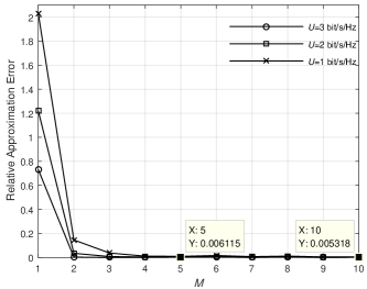
Figure 3: Relative approximate error versus parameter $M$.

Fig. 3 plots the relative approximate error versus parameter $M$ with different settings of $U$ to illustrate the performance of the Gaussian-Chebyshev quadrature approximation approach. Specifically, according to [29], the relative approximation error can be computed as

$$\delta=\left|{\frac{{{\rm{analytical\;result}}-{\rm{simulation\;result}}}}{{{\rm{simulation\;result}}}}}\right|,$$ (84)

where the analytical result is achieved by (41) and the simulation result is obtained from Monte-Carlo simulations. As expected, with the increase of $M$, the relative approximation error approaches zero. For example, when $M=5$, the relative approximation error $\delta$ is $0.006115$, which provides enough accuracy for the system outage probability. Thus, our derived expressions based on the Gaussian-Chebyshev quadrature approximation approach can evaluate the outage performance of the investigated network effectively.

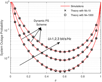
Figure 4: System outage probability versus $\theta$ under dynamic PS scheme.

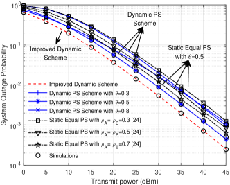
Figure 5: System outage probability versus transmit power $P$.

Fig. 4 plots the system outage probability under the dynamic PS scheme versus the power allocation ratio $\theta$ with $U=1,2$, and $3$ bit/s/Hz, respectively. It can be observed that the theoretical results match with Monte Carlo simulation results with $M=10$ well, which demonstrates the correctness of our derived system outage probability $P_{\rm{out}}^{s}$ in (41). Another observation is that the system outage probability decreases first, reaches the minimum, and then increases. So there exists an optimal $\theta$, which can bring a minimum $P_{\rm{out}}^{s}$. It is worth emphasizing that $\theta=0.5$ assumed in [24] can not yield the minimum $P_{\rm{out}}^{s}$, and that the minimum $P_{\rm{out}}^{s}$ can be achieved by choosing a proper value of $\theta$. Motivated by this, taking the combining strategy of the relay into account, we propose the improved dynamic scheme to reduce the system outage probability further.

Fig. 5 plots the system outage probability as a function of the transmit power, where three schemes are employed, namely, the proposed improved dynamic scheme, the proposed dynamic PS scheme, and the existing static equal scheme in [24]. Specifically, for the improved dynamic scheme, the system outage probability is given by (IV-B). For the dynamic PS scheme, the power allocation ratio is set to be $0.3$, $0.5$, and $0.8$, respectively. For the static equal scheme, according to [24], the power allocation ratio is assumed as $0.5$ and $\rho_{A}=\rho_{B}$ is set as $0.3$, $0.5$, and $0.7$, respectively. As shown in Fig. 5, it can be observed that the system outage probability under the three schemes decreases with the increase of the transmit power and our derived system outage probability under the improved dynamic scheme also perfectly matches the simulation result, which demonstrates the correctness of (IV-B). With the set of $\theta=0.5$, the dynamic PS scheme enjoys a lower outage probability compared with the static equal scheme in [24]. This is because that the dynamic PS scheme can adjust the PS ratios according to the instantaneous CSI to achieve a lower outage probability. For the dynamic PS scheme with $\theta\neq 0.5$, we can see that the static equal scheme in [24] may be superior to the dynamic PS scheme in terms of outage performance. For example, the static equal scheme with $\rho_{A}=\rho_{B}=0.7$ achieves a lower outage probability than the dynamic PS scheme with $\theta=0.3$ or $0.8$. This demonstrates the importance of choosing a proper power allocation ratio $\theta$. Another observation is that the proposed improved dynamic scheme can achieve the best outage performance among the three schemes. This is due to the fact that the proposed improved dynamic scheme takes the optimal dynamic PS ratios and the optimal combining strategy into account and can utilize the instantaneous CSI more effectively. Furthermore, it can also be seen that the slope of system outage probability with the dynamic PS scheme (or the improved dynamic scheme) increases with the transmit power and approaches one when the transmit power is large enough, which verifies our diversity gain analysis in Section III.D and Section IV.D.

Fig. 6 shows the system outage probability for the three schemes versus the $A$-$R$ link distance $d_{A}$ to depict the effect of the relay location on the system outage probability. The transmission rate $U$ is set as $3\;\rm{bit/s/Hz}$. As shown in Fig. 6, it can be observed that with the increase of $d_{A}$, the system outage probability increases first, reaches the maximum value and then decreases. This is due to the fact that the total harvested energy is higher when the relay is closer to either of the terminals. This illustrates that the optimal relay location should be close to either of the terminals to achieve a lower system outage probability. Another observation is that with the same set of $\theta$, the dynamic PS scheme is always superior to the existing static equal scheme in [24] and the improved dynamic scheme outperforms the dynamic PS scheme in terms of the outage performance.

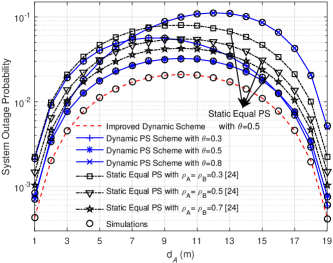
Figure 6: System outage probability versus the $A$-$R$ link distance $d_{A}$ with $U=3\;\rm{bit/s/Hz}$.

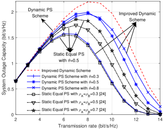
Figure 7: System outage capacity versus transmission rate $U$.

Fig. 7 plots the system outage capacity under three schemes versus the transmission rate $U$. Note that, for the improved dynamic scheme, the system outage capacity is given by (IV-C), while for the dynamic PS scheme with $\theta=0.3$, $0.5$ or $0.8$, the system outage capacity is calculated by (41) and (50). It can be seen that with the increase of $U$, the overall system outage capacity increases first, reaches the peak value and then decreases. The reasons are as follows. With a relatively low transmission rate, the transmission rate $U$ is the dominant factor to the outage capacity. Thus, the outage capacity increases with the increasing of $U$. With a larger transmission rate, the receivers may fail to correctly decode the amount of data. In this case, the outage probability becomes the dominant factor and the outage capacity decreases with the increasing outage probability. Besides, we can see that a well-designed $U$ can bring a higher outage capacity. Another observation is that the improved dynamic scheme can provide a significant performance gain over the dynamic PS schemes and the static equal PS schemes, while with the same set of $\theta$, the dynamic PS scheme always outperforms the static equal PS scheme.

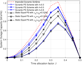
Figure 8: System outage capacity versus time allocation ratio $\beta$ with $P=20$ dBm and $U=5\;\rm{bit/s/Hz}$.

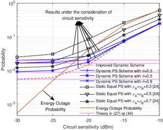
Figure 9: System outage probability and energy outage probability versus circuit sensitivity $P_{\rm{th}}$.

Fig. 8 illustrates the relationship between the system outage capacity and the time allocation ratio $\beta$ with above three schemes considered. We set $P=20$ dBm and $U=5\;\rm{bit/s/Hz}$. One observation is that the system outage capacity increases with the increase of $\beta$ and then decreases. There exists an optimal time allocation ratio $\beta^{*}$ for each scheme to achieve the maximum system outage capacity and $\beta^{*}\geq\frac{1}{3}$. The reason is as follows. When $0<\beta\leq\frac{1}{3}$, the effective transmission time for the system outage capacity is given by $\beta T$ and the system outage capacity increases with increase of $\beta$ due to the fact that a larger $\beta$ yields larger $\gamma_{RA}$ and $\gamma_{RB}$, leading to a lower outage probability. When $\beta>\frac{1}{3}$, the effective transmission time is given by $(1-2\beta)T$. For a larger $\beta$, the effective transmission time becomes the dominant factor to the capacity. Thus, the system outage capacity shows a downward trend. On the other hand, we can also see that the improved dynamic scheme can achieve the highest capacity among the three schemes and with the same set of $\theta$, the dynamic PS scheme is superior to the static equal PS scheme.

Fig. 9 plots the energy outage probability and the system outage probability versus the circuit sensitivity $P_{\rm{th}}$. According to [30], the range of $P_{\rm{th}}$ is set to be $[-30,-10]$ dBm. The energy outage probability is defined as the probability that harvested energy at the relay is $0$. We use $P_{\rm{eo}}$ to denote the energy outage probability. Then we have $P_{\rm{eo}}=\mathbb{P}({P{\rho_{A}}|{h_{A}}{|^{2}}{\Lambda_{A}}d_{A}^{-\alpha}<{P_{{\rm{th}}}}},{P{\rho_{B}}|{h_{B}}{|^{2}}{\Lambda_{B}}d_{B}^{-\alpha}<{P_{{\rm{th}}}}})=\left[{1-\exp\left({-{a_{A}}\left({\frac{{{P_{\rm{th}}}}}{P}+\varpi}\right)}\right)}\right]\left[{1-\exp\left({-{a_{B}}\left({\frac{{{P_{\rm{th}}}}}{P}+\varpi}\right)}\right)}\right]$. For the system outage probability, two cases are considered: (i) the case with $P_{\rm{th}}\neq 0$, (ii) the case with $P_{\rm{th}}=0$. It can be observed that both $P_{\rm{eo}}$ and the system outage probability increase with the increase of $P_{\rm{th}}$ and our derived expressions, (41) and (IV-B), provide lower bounds for the system outage probability in a practical scenario with the circuit sensitivity considered. Specifically, when $P_{\rm{th}}$ is small, the results obtained by our derived expressions of system outage probability are very close to those obtained by considering $P_{\rm{th}}\neq 0$. Besides, we can also see that considering the circuit sensitivity, with the same set of $\theta$, the dynamic PS scheme is still superior to the existing static equal scheme in [24] and the improved dynamic scheme still outperforms the dynamic PS scheme in terms of the outage performance.

VI Conclusions

In this paper, we have proposed two schemes: dynamic PS scheme and improved dynamic scheme, to minimize the system outage probability for the SWIPT enabled three-step DF TWRNs. Specifically, for each scheme, we have derived the optimal solutions in closed forms and further derived the analytical expressions for the optimal system outage probability and capacity. Simulation results validate the correctness of our derived outage probabilities and capacities. The impacts of various parameter settings, e.g., the relay location, the time allocation ratio and the transmission rate, on the system outage performance of SWIPT enabled three-step DF TWRNs have been studied. Several insights have been obtained. First, the proposed schemes are superior to the existing static scheme and the improved dynamic scheme enjoys a lower system outage probability than the dynamic PS scheme. Second, a considerable performance gain can be obtained after carefully selecting a proper time allocation ratio and transmission rate.

Appendix

VI-A Derivation of $F_{t_{2}}(t)$

According to the definition of $F_{t_{2}}(t)$, we have

$$F_{t_{2}}(t)=\mathbb{P}(t_{2}\leq t)=\mathbb{P}\left[{x\leq\left({t-yZ_{B}^{-1}}\right)Z_{A},y\leq tZ_{B}}\right]$$

$$=\int_{0}^{tZ_{B}}{\left[{1-\exp\left({-{a_{A}}\left({t-yZ_{B}^{-1}}\right)}\right)}\right]}\frac{{\exp\left({-{y\mathord{\left/{\vphantom{y{{\lambda_{B}}}}}\right.\kern-1.2pt}{{\lambda_{B}}}}}\right)}}{{{\lambda_{B}}}}dy$$

$$={1-{e^{-{a_{B}}t}}-\frac{{{e^{-{a_{A}}t}}}}{{{\lambda_{B}}}}\int_{0}^{tZ_{B}}{\exp\left({\frac{{{a_{A}}-{a_{B}}}}{{{a_{B}}{\lambda_{B}}}}y}\right)}dy,}\!\!$$ (85)

where $x=|{h_{A}}{|^{2}}$, $y=|{h_{B}}{|^{2}}$ and ${a_{i}}=\frac{{Z_{i}}}{{{\lambda_{i}}}}$. When ${a_{A}}={a_{B}}$, (VI-A) can be computed as

$$F_{t_{2}}(t)={1-{e^{-{a_{B}}t}}-{a_{B}}t{e^{-{a_{A}}t}}}.$$ (86)

For the case with ${a_{A}}\neq{a_{B}}$, (VI-A) is given by

$$F_{t_{2}}(t)={1-{e^{-{a_{B}}t}}-\frac{{{a_{B}}}}{{{a_{A}}-{a_{B}}}}\left({{e^{-{a_{B}}t}}-{e^{-{a_{A}}t}}}\right)}.$$ (87)

Thus, $F_{t_{2}}(t)$ can be rewritten as (38).

VI-B Derivation of $F_{t_{3}}(t)$

Similarly, $F_{t_{3}}(t)$ is given by

$$F_{t_{3}}(t) =\mathbb{P}(x\geq\frac{1}{yt})=\frac{1}{{{\lambda_{B}}}}\int_{0}^{+\infty}{\exp\left({-\frac{1}{{{\lambda_{A}}ty}}-\frac{y}{{{\lambda_{B}}}}}\right)dy}$$

$$=\frac{1}{{{\lambda_{B}}}}\sqrt{\frac{{4{\lambda_{B}}}}{{{\lambda_{A}}t}}}{K_{1}}\left({\sqrt{\frac{4}{{{\lambda_{A}}{\lambda_{B}}t}}}}\right),$$ (88)

where ${K_{1}}\left(\cdot\right)$ is the modified Bessel function of the second kind. The proof is completed.

Liqin Shi received the B.S. degree in electronic information engineering from Sichuan University, Chengdu, China, in 2015. She is currently working toward the Ph.D. degree with the State Key Laboratory of Integrated Service Networks, Xidian University, and a Joint Ph.D. Student with the Department of Electrical and Computer Engineering, Utah State University, UT, USA, under the supervision of Professor Rose Qingyang Hu. Her research interests include wireless energy harvesting, D2D communications, etc. She has published multiple papers in IEEE Transactions on Vehicular Technology, IEEE ICC, etc.

Yinghui Ye received the M.S. degree in communication and information system from Xi’an University of Posts and Telecommunications, Xi an, China, in 2016. Currently, he is working toward the Ph.D. degree with the State Key Laboratory of Integrated Service Networks, Xidian University, and a Joint Ph.D. Student with the Department of Electrical and Computer Engineering, Utah State University, UT, USA, under the supervision of Professor Rose Qingyang Hu. His research interests include cognitive radio networks, relying networks, and wireless energy harvesting. He has authored/coauthored more than twenty technical articles in international journals and proceedings. He is also a reviewer of multiple international Journals and conferences, including the IEEE Transactions on Wireless Communications, the IEEE Transactions on Communications, the IEEE Transactions on Vehicular Technology, the IEEE Internet of Things Journal, the IEEE Communications Letters, the IEEE VTC, etc.

RoseQingyang Hu is a Professor of Electrical and Computer Engineering Department at Utah State University. She received her B.S. degree from University of Science and Technology of China, her M.S. degree from New York University, and her Ph.D. degree from the University of Kansas. She has more than 10 years of R&D experience with Nortel, Blackberry and Intel as a technical manager, a senior wireless system architect, and a senior research scientist, actively participating in industrial 3G/4G technology development, standardization, system level simulation and performance evaluation. Her current research interests include next-generation wireless communications, wireless system design and optimization, green radios, Internet of Things, Cloud computing/fog computing, multimedia QoS/QoE, wireless system modeling and performance analysis. She has published over 180 papers in top IEEE journals and conferences and holds numerous patents in her research areas. Prof. Hu is an IEEE Communications Society Distinguished Lecturer Class 2015-2018 and the recipient of Best Paper Awards from IEEE Globecom 2012, IEEE ICC 2015, IEEE VTC Spring 2016, and IEEE ICC 2016.

Hailin Zhang (M’98) received the B.S. and M.S. degrees from Northwestern Polytechnic University, Xi’an, China, in 1985 and 1988, respectively, and the Ph.D. degree from Xidian University, Xi’an, China, in 1991. In 1991, he joined School of Telecommunications Engineering, Xidian University, where he is now a Senior Professor. He is also currently the Director of Key Laboratory in Wireless Communications sponsored by China Ministry of Information Technology, a key member of State Key Laboratory of Integrated Services Networks, one of the state government specially compensated scientists and engineers, a field leader in Telecommunications and Information Systems in Xidian University, an Associate Director for National 111 Project. Prof. Zhang’s current research interests include key transmission technologies and standards on broadband wireless communications for 5G wireless access systems. He has published more than 100 papers in journals and conferences.

References

• [1] S. M. R. Islam, D. Kwak, M. H. Kabir, M. Hossain, and K. S. Kwak, “The internet of things for health care: A comprehensive survey,” IEEE Access, vol. 3, pp. 678–708, 2015.
• [2] Z. Chu, F. Zhou, Z. Zhu, R. Q. Hu et al., “Wireless powered sensor networks for internet of things: Maximum throughput and optimal power allocation,” IEEE Internet Things J., vol. 5, no. 1, pp. 310–321, Feb 2018.
• [3] W. Guo, S. Zhou, Y. Chen, S. Wang, X. Chu, and Z. Niu, “Simultaneous information and energy flow for IoT relay systems with crowd harvesting,” IEEE Commun. Mag., vol. 54, no. 11, pp. 143–149, November 2016.
• [4] I. Krikidis, S. Timotheou, S. Nikolaou, G. Zheng, D. W. K. Ng, and R. Schober, “Simultaneous wireless information and power transfer in modern communication systems,” IEEE Commun. Mag., vol. 52, no. 11, pp. 104–110, Nov 2014.
• [5] K. Loa, C. c. Wu, S. t. Sheu, Y. Yuan, M. Chion, D. Huo, and L. Xu, “IMT-advanced relay standards,” IEEE Commun. Mag., vol. 48, no. 8, pp. 40–48, August 2010.
• [6] A. Lo, Y. W. Law, and M. Jacobsson, “A cellular-centric service architecture for machine-to-machine (M2M) communications,” IEEE Wireless Commun., vol. 20, no. 5, pp. 143–151, October 2013.
• [7] H. Chen, C. Zhai, Y. Li, and B. Vucetic, “Cooperative strategies for wireless-powered communications: An overview,” IEEE Wireless Commun., pp. 1–8, 2018.
• [8] K. h. Liu and P. Lin, “Toward self-sustainable cooperative relays: state of the art and the future,” IEEE Commun. Mag., vol. 53, no. 6, pp. 56–62, June 2015.
• [9] Y. Ye, Y. Li, F. Zhou, N. Al-Dhahir, and H. Zhang, “Power splitting based swipt with dual-hop DF relaying in the presence of a direct link,” IEEE Syst. J., pp. 1–1, 2018.
• [10] J. Ye, H. Lei, Y. Liu, G. Pan, D. B. da Costa, Q. Ni, and Z. Ding, “Cooperative communications with wireless energy harvesting over nakagami- $m$ fading channels,” IEEE Trans. Commun., vol. 65, no. 12, pp. 5149–5164, Dec 2017.
• [11] A. A. Nasir, X. Zhou, S. Durrani, and R. A. Kennedy, “Relaying protocols for wireless energy harvesting and information processing,” IEEE Trans. Wireless Commun., vol. 12, no. 7, pp. 3622–3636, July 2013.
• [12] Y. Ye, Y. Li, D. Wang, F. Zhou, R. Q. Hu, and H. Zhang, “Optimal transmission schemes for DF relaying networks using SWIPT,” IEEE Trans. Veh. Technol., vol. 67, no. 8, pp. 7062–7072, 2018.
• [13] Y. Liu, L. Wang, M. Elkashlan, T. Q. Duong, and A. Nallanathan, “Two-way relay networks with wireless power transfer: design and performance analysis,” IET Commun., vol. 10, no. 14, pp. 1810–1819, 2016.
• [14] S. Modem and S. Prakriya, “Performance of analog network coding based two-way EH relay with beamforming,” IEEE Trans. Commun., vol. 65, no. 4, pp. 1518–1535, April 2017.
• [15] Z. Chen, B. Xia, and H. Liu, “Wireless information and power transfer in two-way amplify-and-forward relaying channels,” in Proc. IEEE GlobalSIP, Dec 2014, pp. 168–172.
• [16] T. P. Do, I. Song, and Y. H. Kim, “Simultaneous wireless transfer of power and information in a decode-and-forward two-way relaying network,” IEEE Trans. Wireless Commun., vol. 16, no. 3, pp. 1579–1592, March 2017.
• [17] A. Alsharoa, H. Ghazzai, A. E. Kamal, and A. Kadri, “Optimization of a power splitting protocol for two-way multiple energy harvesting relay system,” IEEE Trans. Green Commun. Netw., vol. 1, no. 4, pp. 444–457, Dec 2017.
• [18] H. Cao, L. Fu, and H. Dai, “Throughput analysis of the two-way relay system with network coding and energy harvesting,” in Proc. IEEE ICC, May 2017, pp. 1–6.
• [19] A. Alsharoa, H. Ghazzai, A. E. Kamal, and A. Kadri, “Wireless RF-based energy harvesting for two-way relaying systems,” in Proc. IEEE WCNC, April 2016, pp. 1–6.
• [20] C. Zhang, H. Du, and J. Ge, “Energy-efficient power allocation in energy harvesting two-way AF relay systems,” IEEE Access, vol. 5, pp. 3640–3645, 2017.
• [21] S. T. Shah, K. W. Choi, S. F. Hasan, and M. Y. Chung, “Energy harvesting and information processing in two-way multiplicative relay networks,” Electron. Lett., vol. 52, no. 9, pp. 751–753, 2016.
• [22] Z. Wang, Y. Li, Y. Ye, and H. Zhang, “Dynamic power splitting for three-step two-way multiplicative AF relay networks,” in Proc. IEEE VTC-Fall, Sept 2017, pp. 1–5.
• [23] Y. Ye, Y. Li, Z. Wang, X. Chu, and H. Zhang, “Dynamic asymmetric power splitting scheme for SWIPT based two-way multiplicative AF relaying,” IEEE Signal Process. Lett., vol. 25, no. 7, pp. 1014–1018, 2018.
• [24] N. T. P. Van, S. F. Hasan, X. Gui, S. Mukhopadhyay, and H. Tran, “Three-step two-way decode and forward relay with energy harvesting,” IEEE Commun. Lett., vol. 21, no. 4, pp. 857–860, April 2017.
• [25] D. S. Gurjar, U. Singh, and P. K. Upadhyay, “Energy harvesting in hybrid two-way relaying with direct link under nakagami-m fading,” in Proc. IEEE WCNC, April 2018, pp. 1–6.
• [26] L. Shi, W. Chen, Y. Ye, H. Zhang, and R. Hu, “Heterogeneous power-splitting based two-way DF relaying with non-linear energy harvesting,” in Proc. IEEE GLOBECOM, Dec 2018, pp. 1–7.
• [27] M. Ju and I. M. Kim, “Relay selection with ANC and TDBC protocols in bidirectional relay networks,” IEEE Trans. Commun., vol. 58, no. 12, pp. 3500–3511, December 2010.
• [28] Z. Yi, M. Ju, and I. M. Kim, “Outage probability and optimum combining for time division broadcast protocol,” IEEE Trans. Wireless Commun., vol. 10, no. 5, pp. 1362–1367, May 2011.
• [29] C. Zhang, J. Ge, J. Li, Y. Rui, and M. Guizani, “A unified approach for calculating the outage performance of two-way AF relaying over fading channels,” IEEE Trans. Veh. Technol., vol. 64, no. 3, pp. 1218–1229, March 2015.
• [30] X. Lu, P. Wang, D. Niyato, D. I. Kim, and Z. Han, “Wireless networks with RF energy harvesting: A contemporary survey,” IEEE Commun. Surveys Tuts, vol. 17, no. 2, pp. 757–789, Secondquarter 2015.
• [31] Y. Lee, Y. Kuo, and J. Huang, “Discussion on applying wireless information and power transfer to relay networks,” IEEE Antennas and Wireless Propagation Letters, vol. 17, no. 9, pp. 1750–1754, Sep. 2018.
• [32] A. Bletsas, A. Khisti, D. P. Reed, and A. Lippman, “A simple cooperative diversity method based on network path selection,” IEEE J. Sel. Areas Commun., vol. 24, no. 3, pp. 659–672, March 2006.
• [33] A. Ribeiro, X. Cai, and G. B. Giannakis, “Symbol error probabilities for general cooperative links,” IEEE Tran. Wireless Commun., vol. 4, no. 3, pp. 1264–1273, May 2005.
• [34] E. Hildebrand, Introduction to numerical analysis.   New York, USA: Dover, 1987.