Approximate Multiparametric Mixed-integer Convex Programming

Abstract

We propose an algorithm for generating explicit solutions of multiparametric mixed-integer convex programs to within a given suboptimality tolerance. The algorithm is applicable to a very general class of optimization problems, but is most useful for hybrid model predictive control, where on-line implementation is hampered by the worst-case exponential complexity of mixed-integer solvers. The output is a simplicial partition which defines a static map from the current state to a suboptimal solution. The primary theoretical contribution of this paper is to introduce a non-zero optimal cost overlap metric which is necessary and sufficient for convergence. The overlap size is also linked to partition complexity. The algorithm is massively parallelizable and our implementation, which is publicly available, is run on a cluster of several hundred processors. Not only does our solution have a deterministic runtime, simulations show that our approach is faster than on-line optimization by up to three orders of magnitude.

I Introduction

Hybrid model predictive control (MPC) handles systems with discrete switches or piecewise affinely approximated nonlinearities like chemical powerplants, pipelines and aerospace vehicles [1, 2, 3]. This requires solving a mixed-integer convex program (MICP), which is hampered by the worst-case exponential complexity of mixed-integer solvers. In this paper, we present a provably convergent algorithm for computing explicit solutions of MICPs with a specified suboptimality tolerance.

Several approaches have been proposed to improve hybrid MPC performance. By leveraging the polynomial runtime complexity of convex solvers, successive convexification is able to solve nonlinear programs in real-time [4]. Recently, the method was extended to handle binary decision making via state-triggered constraints [5]. Hence, at least some MICPs are solvable in real-time. However, this is a local method which may not always converge to a feasible solution.

The traditional method of ensuring real-time MPC performance while guaranteeing convergence and global optimality has been to pre-compute the optimal solution off-line. Various explicit MPC methodologies have been proposed [6]. For MPC laws more complicated than linear or quadratic programs, exact explicit solutions are generally not possible due to non-convexity of common active constraint sets [7]. Instead, approximate solutions have been proposed via local linearization [8] or via optimal cost bounding by affine functions over simplices [7] and hyperrectangles [9]. An approximate explicit solution to mixed-integer quadratic programs has been proposed based on difference-of-convex programming [10] and for MICPs based on local linearization and primal/master subproblems [11].

Our contribution in this paper is twofold. First, we introduce a massively parallelizable algorithm for computing the explicit solution to a very general class of multiparametric MICPs and to within a user-specified suboptimality tolerance. Our implementation is available online (see Section V). Second, we define a novel cost overlap metric and show that it is both the fundamental driver of partition complexity and the quantity whose non-zero value is necessary and sufficient for convergence. To the best of our knowledge, the overlap metric is the best theoretical insight to-date about explicit MPC partition complexity. Furthermore, parallelization of explicit MPC algorithms has not yet been exploited in existing literature.

The paper is organized as follows. Section II defines the class of programs that our algorithm can handle. Section III presents the solution algorithm. Section IV proves its convergence and complexity properties. Section V applies the method to the robust control of a satellite’s position. Section VI concludes with future research directions.

Notation: $\mathbb{I}\triangleq\{0,1\}$ is the binary set and $\mathbb{B}\triangleq\{x:\|x\|_{2}\leq 1\}$ is the unit ball. Matrices are uppercase (e.g. $A$), scalars, vectors and functions are lowercase (e.g. $x$), and sets are calligraphic uppercase (e.g. $\mathcal{S}$). ${\mathop{\mathrm{missing}}{co}}\mathcal{S}$, $\mathcal{S}^{\mathrm{c}}$, $\partial\mathcal{S}$ and $\mathcal{V}(\mathcal{R})$ denote respectively the convex hull, complement, boundary and extreme points (e.g. vertices) of $\mathcal{S}$. The cardinality of a countable set $\mathcal{S}$ is $|\mathcal{S}|$. Given $\mathcal{A}\subseteq\mathbb{R}^{n}$, $b\in\mathbb{R}^{n}$ and $s\in\mathbb{R}$, $\mathcal{A}+b\triangleq\{a+b\in\mathbb{R}^{n}:a\in\mathcal{A}\}$ and $s\mathcal{A}\triangleq\{sa:a\in\mathcal{A}\}$.

II Problem Formulation

Our algorithm can handle any problem that can be formulated as the following multiparametric MICP:

$$V^{*}(\theta)={} \min_{x,\delta}~{}f(\theta,x,\delta)~{}\mathrm{s.t.}$$ (P_θ)

$$g(\theta,x,\delta)=0,~{}h(\theta,x,\delta)\in\mathcal{K},$$

where $\theta\in\mathbb{R}^{p}$ is a parameter, $x\in\mathbb{R}^{n}$ is a decision vector and $\delta\in\mathbb{I}^{m}$ is a binary commutation. The cost function $f:\mathbb{R}^{p}\times\mathbb{R}^{n}\times\mathbb{R}^{m}\to\mathbb{R}$ is jointly convex and the constraint functions $g:\mathbb{R}^{p}\times\mathbb{R}^{n}\times\mathbb{R}^{m}\to\mathbb{R}^{l}$ and $h:\mathbb{R}^{p}\times\mathbb{R}^{n}\times\mathbb{R}^{m}\to\mathbb{R}^{d}$ are affine in their first two arguments. The convex cone $\mathcal{K}=\mathcal{C}_{1}\times\cdots\times\mathcal{C}_{q}\subset\mathbb{R}^{d}$ is a Cartesian product of $q$ convex cones. Examples include the positive orthant, the second-order cone and the positive semidefinite cone. If $\delta$ is fixed, (P_θ) becomes a multiparametric convex program:

$$V^{*}_{\delta}(\theta)={} \min_{x}~{}f(\theta,x,\delta)~{}\mathrm{s.t.} {}_{\theta}^{\delta}$$ (P)

$$g(\theta,x,\delta)=0,~{}h(\theta,x,\delta)\in\mathcal{K}.$$

Let $\Theta^{*}\subseteq\mathbb{R}^{p}$ and $\Theta_{\delta}^{*}\subseteq\Theta^{*}$ denote respectively the parameter sets for which (P_θ) and (P${}_{\theta}^{\delta}$) are feasible. Define the following three maps similarly to [7, 12].

Definition 1.

The optimal map $f_{\delta}^{*}:\Theta^{*}\to\mathbb{I}^{m}$ associates $\theta\in\Theta^{*}$ to any optimal commutation of (P_θ), that is any $\delta\in\{\delta\in\mathbb{I}^{m}:V^{*}(\theta)=V^{*}_{\delta}(\theta)\}$.

Definition 2.

The feasible map $f_{\delta}:\Theta^{*}\to\mathbb{I}^{m}$ associates $\theta\in\Theta^{*}$ to a commutation such that (P${}_{\theta}^{\delta}$) is feasible.

Definition 3.

The suboptimal map $f_{\delta}^{\epsilon}:\Theta^{*}\to\mathbb{I}^{m}$ associates $\theta\in\Theta^{*}$ to an $\epsilon$-suboptimal commutation $\delta$ such that

$$V^{*}_{\delta}(\theta)-V^{*}(\theta)<\max\{\epsilon_{\mathrm{a}},\epsilon_{\mathrm{r}}V^{*}(\theta)\},$$ (1)

where $\epsilon_{\mathrm{a}}$ and $\epsilon_{\mathrm{r}}$ are the absolute and relative errors.

The next section presents an algorithm for computing $f_{\delta}^{\epsilon}$ over a subset $\Theta\subseteq\Theta^{*}$. It is assumed that $\Theta$ is a full-dimensional convex polytope in vertex representation. One can choose $\Theta$ following the advice of [12, Section IV-C].

III Explicit Solution of (P_θ)

III-A Suboptimal Map Computation

We begin by computing $f_{\delta}^{\epsilon}$ as a simplicial partition $\mathcal{P}\triangleq\{(\mathcal{R}_{i},\delta_{i},\{x_{i,j}^{*}\}_{j=1}^{|\mathcal{V}(\mathcal{R}_{i})|})\}_{i=1}^{P}$ of $\Theta$. Each simplex $\mathcal{R}_{i}$ is associated with an $\epsilon$-suboptimal $\delta_{i}$ and the set $\{x_{i,j}^{*}\}_{j=1}^{|\mathcal{V}(\mathcal{R}_{i})|}$ of optimal decision vectors of (P${}_{\theta}^{\delta}$) at the vertices of $\mathcal{R}_{i}$.

Algorithm 1 stores $f_{\delta}^{\epsilon}$ as a binary tree and computes it as follows. To initialize, all leaves of the binary tree $f_{\delta}$ output by [12, Algorithm 2] are converted into nodes, i.e. elements that have children in the final tree. Lines 4-14 carry out the main work of partitioning the simplex-commutation tuple $(\mathcal{R},\delta)$. First, the algorithm checks if $\delta$ is $\epsilon$-suboptimal in $\mathcal{R}$. If it is not, the following mixed-integer program must be feasible due to (1):

$$\delta^{*},\theta^{*}={} \mathop{\rm find}_{\theta\in\mathcal{R}}~{}\delta^{\prime}~{}\mathrm{s.t.} \textnormal{E}_{\delta}^{\mathcal{R}}$$ ()

$$V_{\delta}^{*}(\theta)-V_{\delta^{\prime}}^{*}(\theta)\geq\max\{\epsilon_{\mathrm{a}},\epsilon_{\mathrm{r}}V_{\delta^{\prime}}^{*}(\theta)\}.$$

The costs $V_{\delta}^{*}$ and $V_{\delta^{\prime}}^{*}$ are convex [12, Lemma 1]. However, $V_{\delta}^{*}$ appears on the wrong side of the inequality. Hence, ($\textnormal{E}_{\delta}^{\mathcal{R}}$) is non-convex and so is not readily solvable. As a remedy, we formulate a conservative convex upper bound.

Definition 4.

Let $v_{i}\in\mathcal{V}(\mathcal{R})$ be the $i$-th vertex of $\mathcal{R}$ and let $\theta=\sum_{i=1}^{|\mathcal{V}(\mathcal{R})|}\alpha_{i}v_{i}$ where $\alpha_{i}\geq 0$ and $\sum_{i=1}^{|\mathcal{V}(\mathcal{R})|}\alpha_{i}=1$. The affine over-approximator of $V^{*}_{\delta}(\theta)$ over $\mathcal{R}$ is:

$$\bar{V}_{\delta}(\theta)\triangleq\sum_{i=1}^{|\mathcal{V}(\mathcal{R})|}\alpha_{i}V^{*}_{\delta}(v_{i}).$$ (2)

Since $V_{\delta}^{*}$ is convex, $V_{\delta}^{*}(\theta)\leq\bar{V}_{\delta}(\theta)$ $\forall\theta\in\mathcal{R}$. Hence, the following problem is convex and “conservative” in the sense of Theorem 1:

$$\delta^{*},\theta^{*}={} \mathop{\rm find}_{\theta\in\mathcal{R}}~{}\delta^{\prime}~{}\mathrm{s.t.} \bar{\textnormal{E}}_{\delta}^{\mathcal{R}}$$ ()

$$\bar{V}_{\delta}(\theta)-V_{\delta^{\prime}}^{*}(\theta)\geq\max\{\epsilon_{\mathrm{a}},\epsilon_{\mathrm{r}}V_{\delta^{\prime}}^{*}(\theta)\}.$$

Theorem 1.

If ($\bar{\textnormal{E}}_{\delta}^{\mathcal{R}}$) is infeasible then $\delta$ is $\epsilon$-suboptimal.

Proof.

If $\delta$ is not $\epsilon$-suboptimal then ($\textnormal{E}_{\delta}^{\mathcal{R}}$) is feasible, hence ($\bar{\textnormal{E}}_{\delta}^{\mathcal{R}}$) is feasible. By contraposition, if ($\bar{\textnormal{E}}_{\delta}^{\mathcal{R}}$) is infeasible then $\delta$ must be $\epsilon$-suboptimal. ∎

Since ($\bar{\textnormal{E}}_{\delta}^{\mathcal{R}}$) is a MICP, its feasibility can be certified with a mixed-integer solver. If ($\bar{\textnormal{E}}_{\delta}^{\mathcal{R}}$) is infeasible, line 5 converts the node to a leaf since no further partitioning is necessary. Otherwise, we cannot conclude about the $\epsilon$-suboptimality of $\delta$. In this case, we search for a potentially better commutation $\delta^{*}$ via the following extension of ($\bar{\textnormal{E}}_{\delta}^{\mathcal{R}}$):

$$\begin{aligned} \delta^{*},\theta^{*}=~{}&\mathop{\rm find}_{\theta\in\mathcal{R}}~{}\delta^{\prime}~{}\mathrm{s.t.}\\ &\bar{V}_{\delta}(\theta)-V_{\delta^{\prime}}^{*}(\theta)\geq\max\{\epsilon_{\mathrm{a}},\epsilon_{\mathrm{r}}V_{\delta^{\prime}}^{*}(\theta)\},\\ &\delta^{\prime}\in\{\delta^{\prime\prime}\in\mathbb{I}^{m}\setminus\{\delta\}:\mathcal{R}\subseteq\Theta_{\delta^{\prime\prime}}^{*}\}.\end{aligned}, \bar{\textnormal{D}}_{\delta}^{\mathcal{R}}$$ ()

where the last constraint ensures that $\delta^{\prime}$ is feasible in $\mathcal{R}$ and can be embedded via [12, Lemma 2]. If ($\bar{\textnormal{D}}_{\delta}^{\mathcal{R}}$) is infeasible, Section IV shows that a sound strategy is to keep $\delta$ and to split $\mathcal{R}$ in half at the midpoint of its longest edge, as done on line 14. This may also be done if ($\bar{\textnormal{D}}_{\delta}^{\mathcal{R}}$) is feasible since shrinking $\mathcal{R}$ improves the accuracy of the over-approximator (2). However, to avoid unnecessary partitioning, line 8 checks if $V_{\delta}^{*}$ varies over $\mathcal{R}$ by less than the $\epsilon$-suboptimality threshold with respect to $V_{\delta^{*}}(\theta^{*})$ as output by ($\bar{\textnormal{D}}_{\delta}^{\mathcal{R}}$):

$$\max_{\theta\in\mathcal{R}}V_{\delta}^{*}(\theta)-\min_{\theta\in\mathcal{R}}V_{\delta}^{*}(\theta)<\max\{\epsilon_{\mathrm{a}},\epsilon_{\mathrm{r}}V_{\delta^{*}}^{*}(\theta^{*})\},$$ (3)

which can be done with convex optimization. If (3) holds, Theorem 3 assures that $\mathcal{R}$ need not be subdivided further and $\delta^{*}$ is assigned directly on line 9. If (3) does not hold, Section IV shows that a sound strategy is to split $\mathcal{R}$ in half at the midpoint of its longest edge on line 14.

1:Run [12, Algorithm 2] and relabel all leaves as nodes

2:while any nodes exist do

3:   $(\mathcal{R},\delta)\leftarrow\text{the most recently added node}$

4:   if ($\bar{\textnormal{E}}_{\delta}^{\mathcal{R}}$) infeasible then

5:      Change node to leaf $(\mathcal{R},\delta,\{x_{j}^{*}\}_{j=1}^{|\mathcal{V}(\mathcal{R})|})$

6:   else

7:      $\delta^{*},\theta^{*}\leftarrow\text{solve \eqref{eq:better_delta_selection}}$

8:      if ($\bar{\textnormal{D}}_{\delta}^{\mathcal{R}}$) feasible and (3) holds then

9:         Change node to $(\mathcal{R},\mathcal{\delta}^{*})$

10:      else

11:         $\delta^{*}\leftarrow\delta\text{ if \eqref{eq:better_delta_selection} infeasible}$

12:         $v_{1},v_{2}\leftarrow\arg\max_{v,v^{\prime}\in\mathcal{V}(\mathcal{R})}\|v-v^{\prime}\|_{2}$

13:         $\mathcal{S}_{i}\leftarrow{\mathop{\mathrm{missing}}{co}}\{(\mathcal{V}(\mathcal{R})\setminus\{v_{i}\})\cup\{(v_{1}+v_{2})/2\}\},~{}i=1,2$

14:         Add child nodes $(\mathcal{S}_{1},\delta^{*})$ and $(\mathcal{S}_{2},\delta^{*})$          

Algorithm 1 Computation of $f_{\delta}^{\epsilon}$.

III-B Explicit Implementation

At this point the partition $\mathcal{P}$ is available. Consider a cell $(\mathcal{R},\delta,\{x_{j}^{*}\}_{j=1}^{|\mathcal{V}(\mathcal{R})|})$ of the partition. We first recognize the following property.

Theorem 2.

Suppose that $\theta\in\mathcal{R}$ and let $v_{j}\in\mathcal{V}(\mathcal{R})$ be the $j$-th vertex of $\mathcal{R}$. One can write $\theta=\sum_{j=1}^{|\mathcal{V}(\mathcal{R})|}\alpha_{j}v_{j}$ where $\alpha_{j}\geq 0$ and $\sum_{j=1}^{|\mathcal{V}(\mathcal{R}_{j})|}\alpha_{j}=1$. Let $\hat{x}\triangleq\sum_{j=1}^{|\mathcal{V}(\mathcal{R})|}\alpha_{j}x_{j}^{*}$ and $\hat{V}_{\delta}(\theta)\triangleq f(\theta,\hat{x},\delta)$. Then $\hat{x}$ is feasible for (P${}_{\theta}^{\delta}$) and

$$\hat{V}_{\delta}(\theta)\leq\bar{V}_{\delta}(\theta).$$ (4)

Proof.

For feasibility, exploit that $g(\cdot,\cdot,\delta)$ and $h(\cdot,\cdot,\delta)$ in (P${}_{\theta}^{\delta}$) are affine. For (4), exploit that $f(\cdot,\cdot,\delta)$ is convex:

$$\hat{V}_{\delta}(\theta)\leq\sum_{j=1}^{\mathclap{|\mathcal{V}(\mathcal{R})|}}\alpha_{j}f(v_{j},x_{j}^{*},\delta)=\sum_{j=1}^{\mathclap{|\mathcal{V}(\mathcal{R})|}}\alpha_{j}V_{\delta}^{*}(v_{j})=\bar{V}_{\delta}(\theta).\qed$$

As a result of (4), ($\bar{\textnormal{E}}_{\delta}^{\mathcal{R}}$) continues to be infeasible if $\bar{V}_{\delta}(\theta)$ is substituted by $\hat{V}_{\delta}(\theta)$. Therefore $\hat{x}$ is $\epsilon$-suboptimal, i.e.

$$\hat{V}_{\delta}(\theta)-V^{*}(\theta)<\max\{\epsilon_{\mathrm{a}},\epsilon_{\mathrm{r}}V^{*}(\theta)\}.$$ (5)

Hence, given $\theta\in\mathcal{R}\subseteq\Theta$, $\hat{x}$ in Theorem 2 gives an explicit solution and is obtained by querying the partition via:

$$\hat{x}=\sum_{j=1}^{\mathclap{|\mathcal{V}(\mathcal{R})|}}\alpha_{j}x_{j}^{*}\text{ where }\theta=\sum_{j=1}^{\mathclap{|\mathcal{V}(\mathcal{R})|}}\alpha_{j}v_{j},~{}v_{j}\in\mathcal{V}(\mathcal{R}).$$ (6)

IV Properties

IV-A Convergence

This section proves that Algorithm 1 converges if Assumption 1 holds. Without loss of generality, we restrict the discussion to $\Delta$, the set of feasible commutations in $\Theta$.

Definition 5.

The overlap is the largest $\gamma\geq 0$ such that for each $\theta\in\Theta$, $\exists\delta\in\Delta$ which is $\epsilon$-suboptimal in $(\gamma\mathbb{B}+\theta)\setminus\Theta^{\mathrm{c}}$.

Assumption 1.

The overlap is positive, i.e. $\gamma>0$.

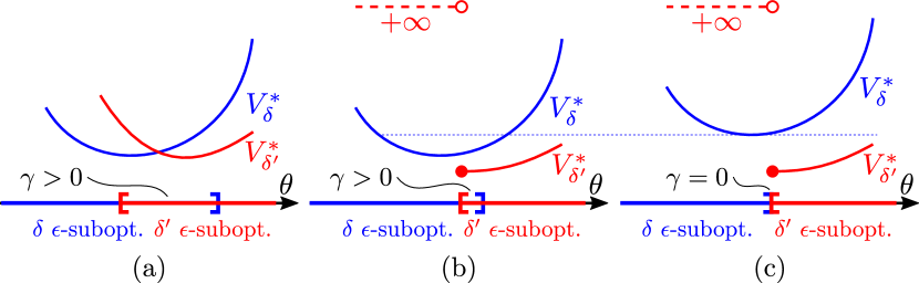
Figure 1: Illustration of “overlap” in Definition 5. In (a) the overlap is positive thanks to local continuity and in (b) it is positive because the downward jump from $V_{\delta}^{*}$ to $V_{\delta^{\prime}}^{*}$ is not too high. In (c) the jump is too high, causing zero overlap.

The overlap $\gamma$ is between sets where a given commutation is $\epsilon$-suboptimal. Its value is a non-trivial property of (P_θ) which increases for larger values of $\epsilon_{\mathrm{a}}$ and $\epsilon_{\mathrm{r}}$. Because Algorithm 1 requires [12, Algorithm 2] to converge, we know that $\gamma\geq 0$ exists. Figure 1 illustrates just three overlap possibilities. For convergence, Algorithm 1 should not “oscillate” between $\delta$ choices for the same $\mathcal{R}$. This is guaranteed by the following lemma.

Lemma 1.

Let $(\mathcal{R},\delta)$ be the node selected on line 3 at some iteration of Algorithm 1. If $\delta$ is replaced with $\delta^{*}$ on line 9, the node $(\mathcal{R},\delta)$ will not reappear in a future iteration.

Proof.

We begin by showing that

$$\min_{\theta\in\mathcal{R}}V_{\delta^{*}}^{*}(\theta)<\min_{\theta\in\mathcal{R}}V_{\delta}^{*}(\theta).$$ (7)

Since ($\bar{\textnormal{D}}_{\delta}^{\mathcal{R}}$) is feasible, $\exists\theta^{*}\in\mathcal{R}$ such that

$$V_{\delta^{*}}^{*}(\theta^{*})\leq\bar{V}_{\delta}(\theta^{*})-\max\{\epsilon_{\mathrm{a}},\epsilon_{\mathrm{r}}V_{\delta^{*}}^{*}(\theta^{*})\}.$$ (8)

Since (3) holds, we have:

$$\bar{V}_{\delta}(\theta^{*}) \leq\max_{\theta\in\mathcal{R}}V_{\delta}^{*}(\theta)$$

$$<\min_{\theta\in\mathcal{R}}V_{\delta}^{*}(\theta)+\max\{\epsilon_{\mathrm{a}},\epsilon_{\mathrm{r}}V_{\delta^{*}}^{*}(\theta^{*})\}.$$ (9)

Substituting (9) into (8) shows that (7) holds. If $(\mathcal{R},\delta)$ reappears in a future iteration, then it must be that all of the preceding iterations finished on line 9. Consider a future iteration where the node is $(\mathcal{R},\tilde{\delta})$. Recursively applying (7), we have:

$$\min_{\theta\in\mathcal{R}}V_{\tilde{\delta}}^{*}(\theta)<\cdots<\min_{\theta\in\mathcal{R}}V_{\delta^{*}}^{*}(\theta)<\min_{\theta\in\mathcal{R}}V_{\delta}^{*}(\theta).$$ (10)

By contradiction, suppose that $\delta$ is chosen on line 7. This means that $\exists\tilde{\theta}\in\mathcal{R}$ such that

$$V_{\delta}^{*}(\tilde{\theta})\leq\bar{V}_{\tilde{\delta}}(\tilde{\theta})-\max\{\epsilon_{\mathrm{a}},\epsilon_{\mathrm{r}}V_{\delta}^{*}(\tilde{\theta})\}.$$ (11)

In the same way that we obtained (9), we have:

$$\bar{V}_{\tilde{\delta}}(\tilde{\theta})<\min_{\theta\in\mathcal{R}}V_{\tilde{\delta}}^{*}(\theta)+\max\{\epsilon_{\mathrm{a}},\epsilon_{\mathrm{r}}V_{\delta}^{*}(\tilde{\theta})\}.$$ (12)

Using (12) in (11), we have

$$V_{\delta}^{*}(\tilde{\theta})<\min_{\theta\in\mathcal{R}}V_{\tilde{\delta}}^{*}(\theta)~{}\Rightarrow~{}\min_{\theta\in\mathcal{R}}V_{\delta}^{*}(\theta)<\min_{\theta\in\mathcal{R}}V_{\tilde{\delta}}^{*}(\theta),$$

which contradicts (10), hence $\delta$ cannot be more optimal than $\tilde{\delta}$ and thus cannot be re-associated with $\mathcal{R}$. ∎

Theorem 3.

Algorithm 1 terminates if and only if Assumption 1 holds.

Proof.

Suppose that Assumption 1 holds. The algorithm terminates when all nodes become leaves. An iteration can exit on line 5, 9 or 14. Since exiting on line 5 terminates a branch, it is necessary and sufficient to show that only a finite number of iterations can exit on lines 9 or 14. Since $V_{\delta}^{*}$ is convex, it is continuous and therefore (3) holds for a small enough $\mathcal{R}$ but with a non-empty interior [13, 14]. If an iteration exits on line 14, the volume of $\mathcal{R}$ is halved and its size is reduced, so after a finite number of iterations $\mathcal{R}$ will be small enough such that (3) holds and $\mathcal{R}\subset\gamma\mathbb{B}+\theta$ for some $\theta\in\Theta$. Once this occurs, by Definition 5 $\exists\delta^{*}\in\Delta$ such that ($\bar{\textnormal{D}}_{\delta}^{\mathcal{R}}$) is feasible. As a result, for any $\delta\in\Delta$ it will take a finite number of iterations until all iterations persistently exit on line 9. However, by Lemma 1 and since $|\Delta|$ is finite, this can only occur a finite number of times. Thus, after a finite number of iterations there will remain only one possible choice of $\delta$ and the iteration will exit on line 5, so the algorithm terminates. If Assumption 1 does not hold, it will take infinite iterations until $\mathcal{R}\subset\gamma\mathbb{B}+\theta$, so the algorithm does not terminate. ∎

Theorem 3 indicates that the partition complexity is driven by $\gamma$ and the required “smallness” of $\mathcal{R}$ such that (3) holds. We formally define the latter quantity below.

Definition 6.

The (conservative) variability is the largest $\nu>0$ such that (3) holds for any $\delta\in\Delta$, any $\mathcal{R}\subset\nu\mathbb{B}+\theta$, any $\theta\in\Theta$ and any $\theta^{*}\in\mathcal{R}$.

Combining Definitions 5 and 6, we can state an overall condition number:

$$\psi\triangleq\min\{\gamma,\nu\}^{-1},$$ (13)

which is positively correlated to how much $\mathcal{R}$ must be subdivided until Theorem 3 assures convergence. We call (P_θ) with small $\psi$ “well-conditioned” and Algorithm 1 will converge faster. Note that larger $\epsilon_{\mathrm{a}}$ and $\epsilon_{\mathrm{r}}$ decrease $\psi$.

IV-B Complexity

This section proves that evaluating (6) has polynomial complexity. We assume that $\Theta$ is a simplex, so the partition $\mathcal{P}$ is a binary tree. We begin by determining the tree depth.

Lemma 2.

The depth $\tau$ of the tree output by Algorithm 1 is $\mathcal{O}(p^{2}\log(\psi))$.

Proof.

In the worst case, Algorithm 1 has to reduce the size of $\mathcal{R}$ until $\mathcal{R}\subset\psi\mathbb{B}+\theta$ for some $\theta\in\Theta$. Once this occurs, Theorem 3 assures that a future iteration will close the corresponding branch without further subdivision. It was shown in [12, Theorem 2] that reducing $\mathcal{R}$ until $\mathcal{R}\subset\psi\mathbb{B}+\theta$ takes $\tau=\mathcal{O}(p^{2}\log(\psi))$ subdivisions. ∎

Theorem 4.

The evaluation complexity of (6) is $\mathcal{O}(p^{4})$.

Proof.

As explained in Section V-A, checking if $\theta\in\mathcal{R}$ can be done via a matrix-vector product, which is $\mathcal{O}(p^{2})$. Since there are $\tau$ such checks to perform and since $\tau=\mathcal{O}(p^{2})$ due to Lemma 2, it takes $\mathcal{O}(p^{4})$ operations to find the $\mathcal{R}$ which contains $\theta$. It subsequently takes $\mathcal{O}(p)$ operations to compute $\hat{x}$, hence the overall evaluation complexity is $\mathcal{O}(p^{4})$. ∎

Theorem 4 stands in contrast to implementing (P_θ) directly with a mixed-integer solver, which has an exponential runtime $\mathcal{O}(2^{m})$.

V Simulation Examples

This section presents two examples to corroborate the effectiveness of Algorithm 1 and the conclusions of Section IV. We consider robust hybrid MPC of a satellite’s out-of-plane (cwh_z) and in-plane (cwh_xy) position. Explicit MPC is relevant for satellite control because the conservative design of space systems typically prohibits the use of on-line optimization. We use Clohessy-Wiltshire-Hill dynamics:

cwh_xy: $$\left\{\begin{array}[]{@{}ll@{}}\ddot{x}=3\omega_{0}^{2}x+2\omega_{o}\dot{y}+u_{x}+w_{x},\\ \ddot{y}=-2\omega_{o}\dot{x}+u_{y}+w_{u},\end{array}\right.$$ (16)

cwh_z: $$\hskip 9.24713pt\ddot{z}=-\omega_{o}^{2}z+u_{z}+w_{z},$$ (17)

where $\omega_{o}$ is the orbital rate in rad/s and $w$ are disturbance terms. The full explanation is provided in [15]. For cwh_xy, the state is $(x,\dot{x},y,\dot{y})\in\mathbb{R}^{4}$ and the input is $(u_{x},u_{y})\in\mathbb{R}^{2}$. For cwh_z, the state is $(z,\dot{z})\in\mathbb{R}^{2}$ and the input is $u_{z}\in\mathbb{R}$. Assuming an impulsive input, the system is discretized at a $T_{\mathrm{s}}=100$ s thruster firing period. On top of [15], we add a lower-bound constraint $\|u\|_{\infty}\geq u_{\min}$ on the thrust magnitude, which arises from the thruster impulse-bit. The constraint is non-convex but can be modeled as the union of convex sets, as illustrated in Figure 2, yielding a mixed-integer second order cone program. We use a prediction horizon $N=4$ and, letting $\mathcal{X}\triangleq[-10,10]~{}\text{cm}\times[-1,1]~{}\text{mm/s}$, choose $\Theta=\mathcal{X}$ for cwh_z and $\Theta=\mathcal{X}\times\mathcal{X}$ for cwh_xy. It was shown in [15] that this $\Theta$ choice is a robust controlled invariant set, hence the partition will be sufficient for controlling the satellite.

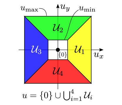
Figure 2: A non-convex input lower-bound constraint for satellite MPC can be modeled as the union of convex sets. This induces a mixed-integer program.

Our implementation is available online and uses Python 3.7.2, CVXPY 1.0.21 [16] and MOSEK 9.0.87 [17]. Recognizing that lines 4-14 can run in parallel across tree branches, we used MPICH 3.2 in CentOS 7 on a cluster of up to 420 2.4 GHz Intel E5-2680 CPU cores with 20 GB of RAM per compute node (28 cores). The code can also run locally.

Example	$s_{\mathrm{a}}$	$\epsilon_{\mathrm{r}}$	$\tau$	$\lambda$	$T_{\mathrm{wall}}$ [hr]	$T_{\mathrm{cpu}}$ [hr]	$M$ [MB]
cwh_z	$0.50$	$2.00$	$13$	$101$	$0.01$	$0.09$	$<0.01$
cwh_z	$0.25$	$1.00$	$17$	$978$	$0.06$	$0.96$	$<0.01$
cwh_z	$0.10$	$0.10$	$20$	$13500$	$0.31$	$7.72$	$11$
cwh_z	$0.03$	$0.05$	$26$	$235231$	$1.91$	$154.19$	$202$
cwh_z	$0.01$	$0.01$	$31$	$3322941$	$6.37$	$2516.98$	$2916$
cwh_xy	$0.50$	$2.00$	$32$	$30448$	$0.57$	$53.44$	$36$
cwh_xy	$0.25$	$1.00$	$49$	$884323$	$3.38$	$1297.35$	$1069$

TABLE I: Numerical results for several $\epsilon$-suboptimality settings; $\tau$ is the tree depth, $\lambda$ is the leaf count, $T_{\mathrm{wall}}$ is the Algorithm 1 runtime, $T_{\mathrm{cpu}}$ is the computation time summed across parallel processors, and $M$ is the tree file size.

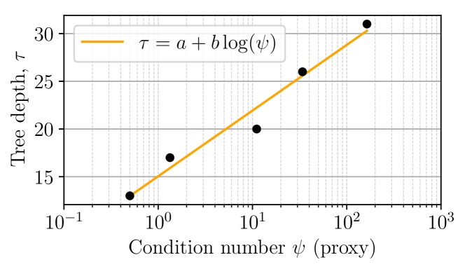
Figure 3: The tree depth for cwh_z is approximately logarithmic in the condition number $\psi$, as predicted by Lemma 2.

Table I summarizes the output of Algorithm 1 using a sequence of increasingly tight $\epsilon$-suboptimality settings. We compute $\epsilon_{a}$ as the largest cost among the vertices of a shrunk $\Theta$, i.e. $\epsilon_{\mathrm{a}}=\max\{V^{*}(\theta)\mid\theta\in\mathcal{V}(s_{\mathrm{a}}\Theta)\}$. The smaller $s_{\mathrm{a}}$ is, the more dense the partition will be in a neighborhood of the origin. Figure 4 shows the progress of Algorithm 1 for the last row of Table I. We can see that the progress is mostly linear. Because multiple cores do not participate in evaluating lines 4-14 for the same node $(\mathcal{R},\delta)$, progress slows down near the end when only a few nodes are left.

Figure 3 confirms that $\tau=\mathcal{O}(\log(\psi))$ using the proxy $\psi=(\epsilon_{\mathrm{a}}/\bar{\epsilon}_{\mathrm{a}}+\epsilon_{\mathrm{r}}/\bar{\epsilon}_{\mathrm{r}})^{-1}$, where $\bar{\epsilon}_{\mathrm{a}}$ and $\bar{\epsilon}_{\mathrm{r}}$ are the largest of the tested values. The leaf count is exponential in $\psi$. It follows that $T_{\mathrm{cpu}}$ and $M$ are also exponential in $\psi$. Note that the exponential increase in $T_{\mathrm{cpu}}$ can be offset by an exponential increase in parallel core count, until a certain limit. Thus, our method allows for reasonable $T_{\mathrm{wall}}$ runtimes.

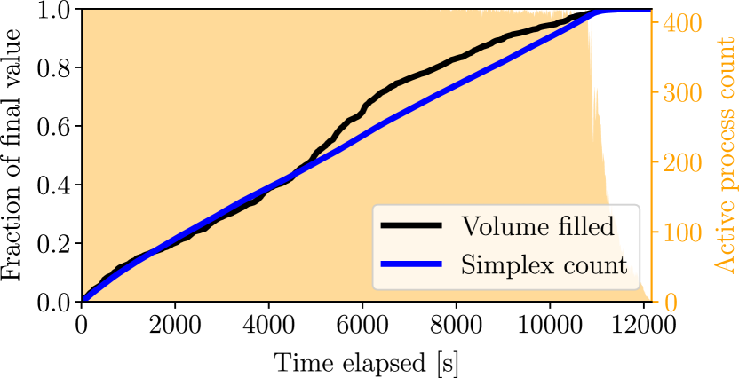
Figure 4: Algorithm 1 progress plot. The partition complexity and the volume fraction of $\Theta$ comprised by completed tree branches steadily increase. The partitioning becomes serialized near the end.

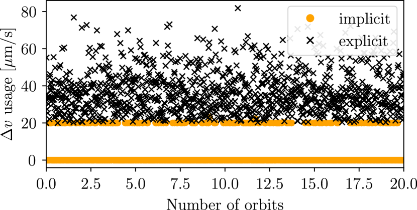
(a) Input 2-norm history for cwh_z with $s_{\mathrm{a}}=0.5$ and $\epsilon_{\mathrm{r}}=2$.

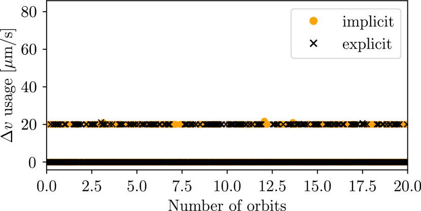
(b) Input 2-norm history for cwh_z with $s_{\mathrm{a}}=0.01$ and $\epsilon_{\mathrm{r}}=0.01$.

Figure 5: Comparison of control input histories for a coarse and a refined $\epsilon$-suboptimal partition. By reducing $\epsilon_{\mathrm{a}}$ and $\epsilon_{\mathrm{r}}$, explicit MPC approaches the behavior of implicit MPC.

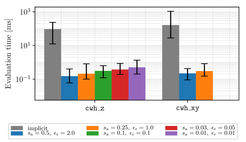
(a) MPC on-line evaluation time. Bars show the mean while error bars shown the minimum and maximum values.

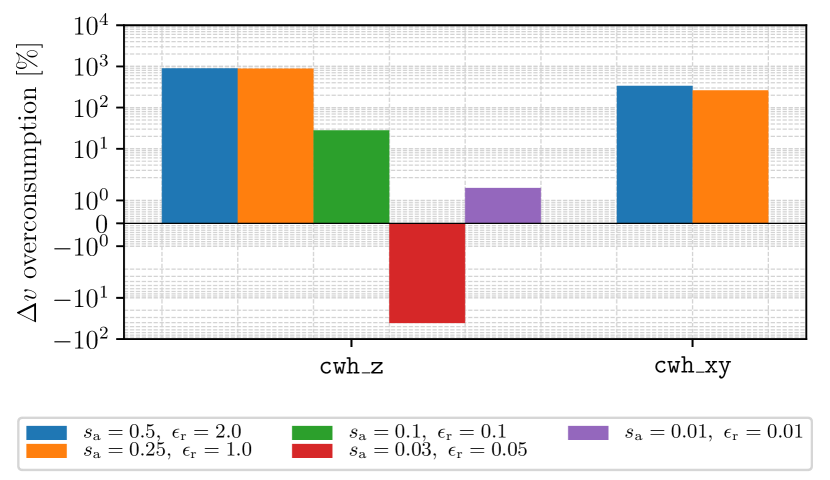
(b) Overconsumption of fuel with respect to implicit MPC due to $\epsilon$-suboptimality. Implicit MPC uses $\approx 4$ mm/s over 20 orbits.

Figure 6: Comparison of the proposed semi-explicit and explicit implementations to implicit MPC in terms of (6(a)) on-line control input computation time and (6(b)) total fuel consumption over $20$ orbits.

Figure 6(a) show statistics for the on-line control input computation time. For implict MPC, this is the mixed-integer solver time. For explicit MPC, it is the time to evaluate (6), which involves querying the partition tree. Statistics are computed by uniformly randomly sampling 1000 values of $\theta\in\Theta$. As expected from Theorem 4, explicit MPC can be up to three orders of magnitude faster. Importantly, explicit MPC provides a real-time guarantee given by the time that it takes to traverse the tree to the deepest leaf. The implicit approach may be arbitrarily slower for some values of $\theta$, subject to the success of the mixed-integer solver’s heuristics.

Figure 6(b) quantifies the fuel consumption suboptimality with respect to implicit MPC. The data is collected based on a 20 orbit simulation where the satellite is initialized at the origin, i.e. with zero control error. As expected, partitions with a tighter $\epsilon$-suboptimality setting perform better. Importantly, explicit MPC can outperform implicit MPC since the control scheme is finite horizon while fuel is an integrated quantity. This is the case for cwh_z with $s_{\mathrm{a}}=0.03$ and $\epsilon_{\mathrm{r}}=0.05$, which achieves $\approx 40~{}\%$ fuel reduction. The source of this reduced fuel consumption is clearly visible in Figure 5, where one can see that with a tighter $\epsilon$-suboptimality setting, explicit MPC better reproduces the optimal behavior of implicit MPC.

V-A Improving the Storage Memory Requirement

Our implementation is not optimized for storage size, so the $M$ values in Table I are far greater than necessary. A more efficient storage model is as follows. Given a simplex $\mathcal{R}\subset\mathbb{R}^{p}$ and its vertices $v_{i}\in\mathcal{V}(\mathcal{R})$, a parameter $\theta\in\mathcal{R}$ if an only if $\alpha=H_{\mathcal{R}}^{-1}(x-v_{1})\geq 0$, $\bm{1}^{\scriptscriptstyle\mathsf{T}}\alpha\leq 1$, where the $i$-th column of $H_{\mathcal{R}}$ equals $v_{i+1}-v_{1}$. Since $\Theta$ and hence $\mathcal{R}$ are full-dimensional, $H_{\mathcal{R}}$ is invertible. By leveraging mutual exclusivity of the partition cells, we can thus store a matrix $H\in\mathbb{R}^{p\times p}$ and a vector $v_{1}\in\mathbb{R}^{p}$ for each “left” child node. For each leaf, in order to evaluate (6) we store the $p+1$ $\epsilon$-suboptimal decision vectors $x_{j}^{*}$ at its vertices. Assuming a perfect binary tree and that $\Theta$ is a simplex, the improved storage size is:

$$M^{*}\approx\frac{3}{2}\lambda\mu_{\mathrm{f}}p(p+1)+\lambda(p+1)\hat{n}\mu_{\mathrm{f}},$$ (18)

where $\mu_{\mathrm{f}}$ is the floating point size and $\hat{n}\leq n$ is the dimension of the part of the decision vector that is necessary to compute the control input (i.e. the first control input for MPC). For the examples in Table I, $M^{*}$ is 3 to 10 times less than $M$. Greater economy is possible by eliminating further redundancy in the stored vertices and optimal decision vectors.

VI Conclusion and Future Work

This paper presented a partitioning algorithm for generating explicit solutions of a very general class of multiparametric mixed-integer convex programs to within a given suboptimality tolerance. We showed that the positivity of a novel cost function overlap metric is necessary and sufficient for algorithm convergence. To the best of our knowledge, this is the first deep theoretical insight into the fundamental driver of convergence rate and partition complexity of suboptimal explicit MPC. In future work it will be interesting to prove the stability of the resulting control law along the lines of [18] and [19], and to see if the selection of $\epsilon_{\mathrm{a}}$ and $\epsilon_{\mathrm{r}}$ could be automated to ensure convergence.

VII Acknowledgments

This research was partially supported by the National Science Foundation (CMMI-1613235). The use of advanced computational, storage, and networking infrastructure was provided by the Hyak supercomputer system and funded by the STF at the University of Washington. The authors would like to thank Martin Cacan, David S. Bayard, Daniel P. Scharf, Jack Aldrich and Carl Seubert of the NASA Jet Propulsion Laboratory, California Institute of Technology, for their helpful insights and discussions.

References

- [1] A. Bemporad and M. Morari, “Control of systems integrating logic, dynamics, and constraints,” Automatica, vol. 35, pp. 407–427, mar 1999.
- [2] L. Blackmore, B. Açıkmeşe, and J. M. Carson III, “Lossless convexification of control constraints for a class of nonlinear optimal control problems,” Systems & Control Letters, vol. 61, pp. 863–870, aug 2012.
- [3] T. Schouwenaars, Safe trajectory planning of autonomous vehicles. Dissertation (Ph.D.), Massachusetts Institute of Technology, 2006.
- [4] Y. Mao, D. Dueri, M. Szmuk, and B. Açıkmeşe, “Successive convexification of non-convex optimal control problems with state constraints,” IFAC-PapersOnLine, vol. 50, pp. 4063–4069, jul 2017.
- [5] M. Szmuk, T. Reynolds, B. Açıkmeşe, M. Mesbahi, and J. M. Carson III, “A tutorial on successive convexification for real-time rocket landing guidance with state-triggered constraints,” in AIAA Scitech 2019 Forum, American Institute of Aeronautics and Astronautics, jan 2019.
- [6] A. Alessio and A. Bemporad, “A survey on explicit model predictive control,” in Nonlinear Model Predictive Control, pp. 345–369, Springer Berlin Heidelberg, 2009.
- [7] A. Bemporad and C. Filippi, “An algorithm for approximate multiparametric convex programming,” Computational Optimization and Applications, vol. 35, pp. 87–108, mar 2006.
- [8] E. N. Pistikopoulos, M. C. Georgiadis, and V. Dua, eds., Multi‐Parametric Programming: Theory, Algorithms, and Applications, vol. 1. Wiley-VCH Verlag GmbH & Co. KGaA, feb 2007.
- [9] T. A. Johansen, “Approximate explicit receding horizon control of constrained nonlinear systems,” Automatica, vol. 40, pp. 293–300, feb 2004.
- [10] A. Alessio and A. Bemporad, “Feasible mode enumeration and cost comparison for explicit quadratic model predictive control of hybrid systems,” IFAC Proceedings Volumes, vol. 39, no. 5, pp. 302–308, 2006.
- [11] V. Dua and E. Pistikopoulos, “An outer-approximation algorithm for the solution of multiparametric MINLP problems,” Computers & Chemical Engineering, vol. 22, pp. S955–S958, mar 1998.
- [12] D. Malyuta, B. Açıkmeşe, M. Cacan, and D. S. Bayard, “Partition-based feasible integer solution pre-computation for hybrid model predictive control,” in 2019 European Control Conference (accepted), p. arXiv:1902.10989, IFAC, jun 2019.
- [13] S. Boyd and L. Vandenberghe, Convex Optimization. Cambridge University Press, 2004.
- [14] H. Royden, Real Analysis. Pearson, 3 ed., 1988.
- [15] D. Malyuta, B. Açıkmeşe, and M. Cacan, “Robust model predictive control for linear systems with state and input dependent uncertainties,” in 2019 American Control Conference (accepted), p. arXiv:1902.10984, IEEE, jul 2019.
- [16] S. Diamond and S. Boyd, “CVXPY: A Python-embedded modeling language for convex optimization,” Journal of Machine Learning Research, vol. 17, no. 83, pp. 1–5, 2016.
- [17] MOSEK ApS, MOSEK Optimizer API for Python 9.0.87, 2019.
- [18] M. de la Pena, A. Bemporad, and C. Filippi, “Robust explicit MPC based on approximate multi-parametric convex programming,” in 2004 43rd IEEE Conference on Decision and Control (CDC) (IEEE Cat. No.04CH37601), IEEE, 2004.
- [19] D. M. D. L. Pena, A. Bemporad, and C. Filippi, “Robust explicit MPC based on approximate multiparametric convex programming,” IEEE Transactions on Automatic Control, vol. 51, pp. 1399–1403, aug 2006.