Partition-based Feasible Integer Solution Pre-computation for Hybrid Model Predictive Control

Abstract

For multiparametric mixed-integer convex programming problems such as those encountered in hybrid model predictive control, we propose an algorithm for generating a feasible partition of a subset of the parameter space. The result is a static map from the current parameter to a suboptimal integer solution such that the remaining convex program is feasible. Convergence is proven with a new insight that the overlap among the feasible parameter sets of each integer solution governs the partition complexity. The partition is stored as a tree which makes querying the feasible solution efficient. The algorithm can be used to warm start a mixed integer solver with a real-time guarantee or to provide a reference integer solution in several suboptimal MPC schemes. The algorithm is tested on randomly generated systems with up to six states, demonstrating the effectiveness of the approach.

I Introduction

Model predictive control (MPC) is a discrete-time control technique in which a receding horizon optimization problem is solved in order to determine the optimal control input at each time step. Advanced formulations of MPC include hybrid MPC (HMPC) and robust MPC (RMPC) [1, 2, 3]. HMPC handles systems like chemical powerplants, pipelines and aerospace vehicles whose dynamics involve either explicit discrete switches such as valves [4, 5] or have nonlinearities that can be appropriately modeled via a piecewise affine approximation [6, 7]. RMPC handles systems that are affected by uncertainties such as in their dynamics, in the state estimate and in the input [2, 8]. Many practical applications call for a combined control of uncertain hybrid systems which requires solving a convex mixed-integer nonlinear program (MINLP) [9, 10, 11]. While possible on powerful hardware, on-line MINLP solution is both slow and $\mathcal{NP}$-complete [4], meaning that there is generally no real-time performance guarantee.

To improve MPC on-line computational efficiency, some authors have worked on explicit MPC techniques which reduce on-line computational demand by pre-computing off-line all or part of the optimal solution. On-line it typically remains to evaluate a piecewise affine (PWA) function. Various explicit MPC methodologies have been proposed [12, 13, 14]. When the MPC law is a linear or a quadratic program, an exact explicit law can be obtained by solving a multiparametric program. Exact solutions for more general programs are generally not possible due to non-convexity of common active constraint regions [15]. Instead, approximate solutions have been proposed via local linearization [16, 17] or via optimal cost bounding by PWA functions over simplices [15, 18, 19] or hyperrectangles [20]. An approximate explicit solution to mixed-integer quadratic programs has been proposed based on difference of convex programming [21] and for MINLPs based on local linearization and primal/master subproblems [22, 23].

Multiparametric programming, however, is restricted to relatively low dimensional systems due to the worst-case exponential partition complexity. Several authors in hybrid MPC have therefore suggested to retain on-line mixed-integer programming and either to reduce the integer variable’s degrees of freedom [24] or to abort the solver at a suboptimal solution when computation time becomes excessive [4]. The former solution, however, has no rigorous way of selecting a reference integer solution while the latter relies on the ability to use the previous time step’s solution to warm start the mixed-integer solver, which is not always possible such as, for example, in some robust MPC schemes [8].

To address the issue of guaranteed real-time computation of a feasible integer solution in the general setting, our main contribution is a novel partitioning algorithm which pre-computes feasible integer solutions in a polytopic subset of the state space. This partition is stored as a tree which can be queried in polynomial time. As a result, the partition provides a guaranteed real-time warm start capability to the mixed-integer solver and thus is helpful for [4, 24]. Our second contribution is a convergence proof of the algorithm which for the first time in literature considers an overlap property as being a driver of partition complexity.

The paper is organized as follows. In Section II the scope of MPC formulations that our algorithm can handle is defined as a generic MINLP. The algorithm is then described in Section III and its convergence, complexity and use-cases are discussed in Section IV. The algorithm is tested on a large set of randomly generated dynamical systems with up to 6 states and 21 integer variable degrees of freedom, indicating that it is robust and can scale to medium dimensional systems. Section VI outlines future research directions and is followed by some concluding remarks in Section VII.

II Problem Formulation

This section defines a template MINLP that generates all MPC laws that our algorithm can handle. Because MPC is fundamentally an optimization problem, we do this without specific mention of a receding-horizon optimal control problem.

We use the following notation. $\mathbb{R}$ denotes the set of reals, $\mathbb{I}\triangleq\{0,1\}$ the binary set and $\mathbb{B}\triangleq\{x:\|x\|_{2}\leq 1\}$ the unit ball. Unless otherwise specified, matrices are uppercase (e.g. $A$), scalars, vectors and functions are lowercase (e.g. $x$) and sets are calligraphic uppercase (e.g. $\mathcal{S}$). We use $1_{n}\in\mathbb{R}^{n}$ to denote the vector of ones and $I_{n}\in\mathbb{R}^{n\times n}$ to denote the identity matrix. The scalar $\ell$ is a placeholder for some integer value. The operator $\mathrm{diag}(\{x_{i}\}_{i=1}^{\ell})\in\mathbb{R}^{\ell\times\ell}$ creates a diagonal matrix with value $x_{i}$ at row and column $i$ and zero otherwise. The constraint $M\succ(\succeq)0$ means that $M\in\mathbb{R}^{n\times n}$ is positive (semi)definite. $\mathcal{S}^{\mathrm{c}}$, $\partial\mathcal{S}$, $c^{\mathcal{S}}$ and $\mathcal{V}(\mathcal{S})$ denote respectively the complement, boundary, barycenter and vertices of $\mathcal{S}$ (with the latter only relevant when $\mathcal{S}$ is a polytope). Given $\mathcal{A}\subseteq\mathbb{R}^{n}$, $s\in\mathbb{R}$ and $b\in\mathbb{R}^{n}$, $\mathcal{A}+b\triangleq\{a+b\in\mathbb{R}^{n}:a\in\mathcal{A}\}$ translates and $s\mathcal{A}\triangleq\{sa:a\in\mathcal{A}\}$ scales the set $\mathcal{A}$. The shorthand $a:b$ denotes the integer sequence $a,\dots,b$.

The following multiparametric conic MINLP generates all MPC formulations that our algorithm can handle:

$$V^{*}(\theta) = \min_{x,\delta}\text{ } f(\theta,x,\delta)$$ (P_θ)

$$\mathrm{s.t.}\text{ } g(\theta,x,\delta)=0,$$

$$h(\theta,x,\delta)\in\mathcal{K},$$

$$\delta\in\mathbb{I}^{m},$$

where $\theta\in\mathbb{R}^{p}$ is the parameter, $x\in\mathbb{R}^{n}$ is the decision vector and $\delta\in\mathbb{I}^{m}$ is a binary vector called the commutation. The cost function $f:\mathbb{R}^{p}\times\mathbb{R}^{n}\times\mathbb{I}^{m}\to\mathbb{R}$ is jointly convex in its first two arguments while the constraint functions $g:\mathbb{R}^{p}\times\mathbb{R}^{n}\times\mathbb{I}^{m}\to\mathbb{R}^{\ell}$ and $h:\mathbb{R}^{p}\times\mathbb{R}^{n}\times\mathbb{I}^{m}\to\mathbb{R}^{d}$ are affine in their first two arguments. The functions can be nonlinear in the last argument. The convex cone $\mathcal{K}=\mathcal{C}_{1}^{c_{1}}\times\cdots\times\mathcal{C}_{q}^{c_{q}}\subset\mathbb{R}^{d}$ is a Cartesian product of $q$ convex cones where $\mathcal{C}_{i}^{c_{i}}\subset\mathbb{R}^{c_{i}}$ and $d\triangleq\sum_{i=1}^{q}c_{i}$, similar to [25]. Examples include the positive orthant $\mathbb{R}_{+}^{n}$, the second-order cone $\mathcal{Q}^{\ell}=\{(t,z)\in\mathbb{R}\times\mathbb{R}^{\ell-1}:t\geq\|z\|_{2}\}$ and the positive semidefinite cone $\mathcal{S}_{+}^{\ell}=\{Z\in\mathbb{R}^{\ell\times\ell}:Z\succeq 0\}$. We also define the following fixed-commutation multiparametric conic NLP:

$$V^{*}_{\delta}(\theta) = \min_{x}\text{ } f(\theta,x,\delta) {}_{\theta}^{\delta}$$ (P)

$$\mathrm{s.t.}\text{ } g(\theta,x,\delta)=0,$$

$$h(\theta,x,\delta)\in\mathcal{K},$$

which corresponds to (P_θ) where $\delta$ has been fixed, i.e. assigned a specific value. The following definitions closely follow [15].

Definition 1.

The feasible parameter set $\Theta^{*}\subset\mathbb{R}^{p}$ is the set of all $\theta$ parameters for which (P_θ) is feasible.

Definition 2.

The fixed-commutation feasible parameter set $\Theta_{\delta}^{*}\subset\mathbb{R}^{p}$ is the set of all $\theta$ parameters for which (P${}_{\theta}^{\delta}$) is feasible.

Definition 3.

The feasible commutation map $f_{\delta}:\Theta^{*}\to\mathbb{I}^{m}$ maps $\theta\in\Theta^{*}$ to a commutation $\delta$ such that $\theta\in\Theta^{*}_{\delta}$.

This paper presents an algorithm for computing $f_{\delta}$ over a subset of its domain $\Theta\subseteq\Theta^{*}$. We shall assume in Section III that the set $\Theta$ is available as a convex and full-dimensional polytope in vertex representation. Section IV-C discusses how one might obtain $\Theta$. It is implicitly assumed throughout this paper that (P_θ) and all related problems are appropriately scaled. We suggest a per-axis unit scaling such that $\max_{\theta\in\Theta}|e_{i}^{\scriptscriptstyle\mathsf{T}}\theta|=1$ $\forall i=1,\dots,p$ where $\{e_{i}\}_{i=1}^{p}$ is the standard Eucledian basis.

III Feasible Commutation Map Computation

This section proposes an algorithm for computing $f_{\delta}$. The main idea is to generate a coarse simplicial partition $\mathcal{R}=\{(\mathcal{R}_{i},\delta_{i})\}_{i=1}^{|\mathcal{R}|}$ such that $\Theta=\bigcup_{i=1}^{|\mathcal{R}|}\mathcal{R}_{i}$ and where each cell $\mathcal{R}_{i}$ is associated with a fixed commutation $\delta_{i}$ that is feasible everywhere in $\mathcal{R}_{i}$, i.e. $\mathcal{R}_{i}\subseteq\Theta^{*}_{\delta_{i}}$. We then define:

$$f_{\delta}(\theta)=\delta_{i}\text{ such that }\theta\in\mathcal{R}_{i}.$$ (1)

Lemma 1.

For any fixed $\delta\in\mathbb{I}^{m}$, $\Theta^{*}_{\delta}$ is a convex set and $V^{*}_{\delta}$ is a convex function.

Proof.

Suppose $\theta^{\prime},\theta^{\prime\prime}\in\Theta^{*}_{\delta}$. Let $\alpha^{\prime},\alpha^{\prime\prime}\in[0,1]$, $\alpha^{\prime}+\alpha^{\prime\prime}=1$ and $\theta=\alpha^{\prime}\theta^{\prime}+\alpha^{\prime\prime}\theta^{\prime\prime}$. Since $g,h$ are affine in their first argument and $\mathcal{K}$ is a convex cone:

$$\begin{split}g(\theta,x,\delta)=\alpha^{\prime}g(\theta^{\prime},x,\delta)+\alpha^{\prime\prime}g(\theta^{\prime\prime},x,\delta)=0,\\ h(\theta,x,\delta)=\alpha^{\prime}h(\theta^{\prime},x,\delta)+\alpha^{\prime\prime}h(\theta^{\prime\prime},x,\delta)\in\mathcal{K},\end{split}$$

so $\theta\in\Theta^{*}_{\delta}$ which is thus a convex set. Next, (P${}_{\theta}^{\delta}$) is a minimization of $f$ over a convex set in $x$ which preserves convexity in $\theta$ by the joint convexity property of $f$ [26]. Thus, $V^{*}_{\delta}$ is a convex function. ∎

1:$\mathcal{R}\leftarrow\emptyset$, $\bar{\Theta}\leftarrow\Theta$

2:for all $\delta\in\mathbb{I}^{m}$ do

3:   $\mathcal{R}\leftarrow\{(\mathcal{R}^{\prime},\delta):\mathcal{R}^{\prime}\in\bar{\Theta}\cap\Theta^{*}_{\delta}\}\cup\mathcal{R}$

4:   $\bar{\Theta}\leftarrow\bar{\Theta}\setminus\Theta^{*}_{\delta}$

5:   if $\bar{\Theta}=\emptyset$ then

6:      STOP    

Algorithm 1 Brute force $f_{\delta}$ computation.

Since $\Theta^{*}_{\delta}$ is convex, an arbitrarily precise inner approximation of it can be found [27]. A conceptually trivial method for generating $\mathcal{R}$ is given by Algorithm 1. The set difference and intersection operations in Algorithm 1 are element-wise [28]. The idea is to exploit the ability to inner approximate $\Theta^{*}_{\delta}$ to procedurally “cover” $\Theta$ by intersecting it with fixed-commutation feasible parameter sets.

The filling problem is combinatorial, however, such that in the worst case all $2^{m}$ possible values of $\delta$ are needed, excepting those that are infeasible directly due to the constraints in (P_θ). Furthermore, accurate polytopic inner approximation of $\Theta^{*}_{\delta}$ in higher-dimensional spaces than about $\mathbb{R}^{4}$ suffers from excessive vertex count [27]. Last but not least, the set intersection and set difference operations used by Algorithm 1 have poor numerical properties such as creating badly conditioned (i.e. quasi lower-dimensional) polytopes. One would like instead an algorithm which may 1) potentially avoid exploring all $2^{m}$ combinations for $\delta$, 2) minimizes vertex count and 3) uses only numerically robust operations. We thus propose Algorithm 2 in which the first requirement is addressed via (V^R) discussed below, the second by using only simplices (which have the lowest vertex count among full-dimensional polytopes) and the third by working solely in the vertex representation which is much more numerically robust than the halfspace representation and avoids the numerically fragile operation of converting between the two representations.

1:Create empty tree with open leaf $\Theta$ as root

2:$\mathcal{S}\leftarrow\mathtt{delaunay}(\mathcal{V}(\Theta))$

3:Add child open leaves $\mathcal{S}_{i}$ $\forall\mathcal{S}_{i}\in\mathcal{S}$

4:while any open leaf exists do

5:   $\mathcal{R}\leftarrow\text{the first open leaf}$

6:   if (P_θ) is infeasible for $\theta=c^{\mathcal{R}}$ then

7:      STOP, $\Theta^{*}\setminus\Theta\neq\emptyset$

8:   else

9:      $\hat{\delta}\leftarrow\text{solve (\ref{eq:maxvol})}$

10:      if (V^R) is infeasible then

11:         $\bar{v},\bar{v}^{\prime}\leftarrow\arg\max_{v,v^{\prime}\in\mathcal{V}(\mathcal{R})}\|v-v^{\prime}\|_{2}$

12:         $v_{\mathrm{mid}}\leftarrow(\bar{v}+\bar{v}^{\prime})/2$

13:         Add child open leaf ${\mathop{\mathrm{missing}}{co}}\{(\mathcal{V}(\mathcal{R})\setminus\{\bar{v}\})\cup\{v_{\mathrm{mid}}\}\}$

14:         Add child open leaf ${\mathop{\mathrm{missing}}{co}}\{(\mathcal{V}(\mathcal{R})\setminus\{\bar{v}^{\prime}\})\cup\{v_{\mathrm{mid}}\}\}$

15:      else

16:         Replace leaf with closed leaf $(\mathcal{R},\hat{\delta})$          

Algorithm 2 Proposed computation of $f_{\delta}$.

Algorithm 2 creates a simplicial partition of $\Theta$ as follows. The partition is stored as a tree whose leaves are cells $(\mathcal{S},\delta)$ storing the set $\mathcal{S}$ and associated commutation $\delta$. Non-leaf nodes in the tree store just the sets and make evaluating (1) more efficient (see Section IV-B). A “closed leaf” refers to a cell that will be a leaf in the final tree while an “open leaf” will be further partitioned at the next iteration and thus will be merely a non-leaf node in the final tree. In the algorithm, we refer to nodes directly by their contents, i.e. $\mathcal{S}$ for open and $(\mathcal{S},\delta)$ for closed leaves. On line 3 the tree root is initialized to $\Theta$ and, since generally $\Theta$ is not a simplex, Delaunay triangulation is first applied [29, Section 9.3]. The tree is then iterated on line 4 in a depth-first manner until no open leaves are left. By doing a depth-first search, Assumption 1 in Section IV-A is disproved more quickly in case that it does not hold, such that the algorithm fails with less wasted time.

An open leaf $\mathcal{R}$ in the tree is selected on line 5. First, it is checked whether (P_θ) is feasible at its barycenter. If not, this point is a certificate of infeasibility of (P_θ) in $\Theta$, in which case Section IV-C should be consulted. If however (P_θ) is feasible, then lines 9-16 partition $\mathcal{R}$ into at most $2$ simplices. First, it is checked whether $\mathcal{R}$ is fully contained inside some particular $\Theta^{*}_{\delta}$. The following lemma is used for this purpose.

Lemma 2.

$\mathcal{R}\subseteq\Theta^{*}_{\hat{\delta}}$ $\Leftrightarrow$ (P${}_{\theta}^{\delta}$) is feasible $\forall\theta\in\mathcal{V}(\mathcal{R})$ and $\delta=\hat{\delta}$.

Proof.

$(\Rightarrow)$ Since $\mathcal{R}\subseteq\Theta^{*}_{\hat{\delta}}$, $\theta\in\mathcal{V}(\mathcal{R})\Rightarrow\theta\in\Theta_{\hat{\delta}}^{*}$. Since $\Theta_{\hat{\delta}}^{*}$ is the fixed-commutation feasible parameter set, (P${}_{\theta}^{\delta}$) is by definition feasible. $(\Leftarrow)$ Any $\theta$ such that (P${}_{\theta}^{\delta}$) is feasible satisfies, by definition, $\theta\in\Theta^{*}_{\hat{\delta}}$. By Lemma 1, since $\Theta^{*}_{\hat{\delta}}$ is convex, ${\mathop{\mathrm{missing}}{co}}\{\theta\in\mathcal{V}(\mathcal{R})\}\equiv\mathcal{R}\subseteq\Theta^{*}_{\hat{\delta}}$. ∎

Using Lemma 2, one can efficiently check if $\mathcal{R}\subseteq\Theta^{*}_{\delta}$ for some $\delta$ via the following feasibility MINLP:

$$\hat{\delta}(\mathcal{R}) = \operatorname*{find}\text{ } \delta$$ (V^R)

$$\mathrm{s.t.}\text{ } g(\theta,x_{\theta},\delta)=0\quad \forall\theta\in\mathcal{V}(\mathcal{R}),$$

$$h(\theta,x_{\theta},\delta)\in\mathcal{K} \forall\theta\in\mathcal{V}(\mathcal{R}),$$

$$\delta\in\mathbb{I}^{m},$$

where $x_{\theta}$ denotes a feasible decision vector corresponding to the particular value of $\theta$. Problem (V^R) can be solved in the standard fashion as a MINLP and the found feasible commutation can be associated with $\mathcal{R}$ and the leaf can be subsequently closed. If (V^R) is infeasible, however, then $\mathcal{R}$ is not fully contained in any $\Theta^{*}_{\delta}$. In this case, $\mathcal{R}$ is split into two smaller simplices at the midpoint of its longest edge. As explained in Section IV-A, this yields a volume reduction that necessarily leads to convergence if Assumption 1 holds.

IV Properties

IV-A Convergence

The main result of this section is Theorem 1 which guarantees convergence of Algorithm 2 under an assumption.

Definition 4.

Let $\Delta\triangleq\{\delta\in\mathbb{I}^{m}:\Theta^{*}_{\delta}\cap\Theta\neq\emptyset\}$. The largest value $\kappa\in\mathbb{R}_{+}$ such that $\forall\theta\in\Theta$ $\exists\delta\in\Delta$ such that $(\kappa\mathbb{B}+\theta)\setminus(\Theta^{*}\cap\Theta)^{\mathrm{c}}\subseteq\Theta^{*}_{\delta}$ is called the overlap.

Assumption 1.

The overlap is positive, i.e. $\kappa>0$.

The overlap depends on (P_θ) and the choice of $\Theta$. Assumption 1 implies that a non-zero overlap between fixed-commutation feasible parameter sets exists everywhere near $\partial\Theta^{*}_{\delta}$ $\forall\delta\in\Delta$. This “fuzzy” commutation transition property is instrumental for the convergence proof in Theorem 1.

Theorem 1.

If Assumption 1 holds then Algorithm 2 either converges or fails in a finite number of iterations.

Proof.

Let $\mathcal{R}_{k}$ be the leaf chosen at the $k$-th call of line 5. Whenever $\mathcal{R}_{k}$ is not closed, it can be shown that the partition along its longest edge on lines 11-14 halves the volume, therefore $\lim_{k\to\infty}\mathrm{vol}(\mathcal{R}_{k})=0$. Since the longest edge length is also halved, $\exists k$ large enough such that $\mathcal{R}_{k}\subseteq(\kappa\mathbb{B}+c^{\mathcal{R}_{k}})$. Two possibilities exist: 1) $\mathcal{R}_{k}\subseteq(\kappa\mathbb{B}+c^{\mathcal{R}_{k}})\setminus(\Theta^{*}\cap\Theta)^{\mathrm{c}}$ or 2) $\mathcal{R}_{k}\cap(\Theta^{*})^{\mathrm{c}}\neq\emptyset$. In the first case, the $\hat{\delta}$ picked on line 9 is then the one feasible $\forall\theta\in\mathcal{V}(\mathcal{R}_{k})$. Leaf $\mathcal{R}_{k}$ is therefore closed on line 16. By this logic, for a large enough (but finite) $k$ all regions that do not intersect the infeasible parameter set $(\Theta^{*})^{\mathrm{c}}$ get closed. If the second case does not occur, the algorithm terminates.

In the second case, recall that $\lim_{k\to\infty}\mathrm{vol}(\mathcal{R}_{k})=0$. Since $\mathcal{R}_{k}\cap(\Theta^{*})^{\mathrm{c}}\neq 0$, in a finite number of iterations $c^{\mathcal{R}_{k}}\notin\Theta^{*}$ so line 6 will evaluate to true and the algorithm will fail on line 7. ∎

Corollary 1.

If Assumption 1 does not hold then Algorithm 2 does not converge.

Proof.

If Assumption 1 does not hold then there exists a region $\Theta^{\prime}\subseteq\Theta$ such that $\forall\theta\in\Theta^{\prime}$, $(\kappa\mathbb{B}+\theta)\setminus(\Theta^{*}\cap\Theta)^{\mathrm{c}}\subseteq\Theta^{*}_{\delta}$ for some $\delta\in\Delta\Leftrightarrow\kappa=0$. This, however, implies that the only simplex that would validate Lemma 2 is a lower-dimensional one, i.e. with zero volume. Since this occurs at iteration $k=\infty$, Algorithm 2 does not converge. ∎

Theorem 1 and Corollary 1 suggest that $\kappa>0$ is not only necessary and sufficient for convergence but that $\kappa$ also drives the convergence rate. A small $\kappa$ implies a high iteration count $k$ until Assumption 1 guarantees leaf closure. We call a MINLP with large $\kappa$ “well-conditioned” and Algorithm 2 will converge more quickly with a rate that is derived in Corollary 2 of Section IV-B.

IV-B Complexity

In this section we analyze the complexity of Algorithm 2 in terms of the partition cell count as well as the on-line evaluation complexity.

Theorem 2.

The maximum tree depth $\tau$ of Algorithm 2 is $\mathcal{O}(p^{2}\log(\kappa^{-1}))$.

Proof.

Algorithm 2 reduces search space volume by halving the longest edge length on lines 11-14. Suppose that $l_{0}$ is the longest edge length of a simplex $\mathcal{R}\subset\mathbb{R}^{p}$, then its length is $l_{k}\triangleq l_{0}/2^{k}$ after $k$ divisions. We wish to determine the number of divisions necessary until $\mathcal{R}\subseteq\kappa\mathbb{B}+c^{\mathcal{R}}$ and gets closed by Theorem 1. This approximately requires $l_{k}\leq\kappa\Rightarrow k\geq\log_{2}(l_{0}/\kappa)$. Since $\mathcal{R}$ has $p(p+1)/2$ edges then an approximate number of required subdivisions, i.e. the depth of the partition tree, is given by:

$$\tau=\left\lceil\frac{p(p+1)\log_{2}(l_{0}/\kappa)}{2}\right\rceil,$$ (2)

which yields $\tau=\mathcal{O}(p^{2}\log(\kappa^{-1}))$. ∎

Corollary 2.

The maximum tree leaf count $\eta$ of Algorithm 2 is $\mathcal{O}(2^{p^{2}\log(\kappa^{-1})})$.

Proof.

In the worst case, Algorithm 2 generates a full binary tree of depth $\tau=\mathcal{O}(p^{2}\log(\kappa^{-1}))$ according to Theorem 2, neglecting the first layer where the node count depends on $|\mathcal{S}|$ on line 2. Such a tree contains $\eta=2^{\tau}=\mathcal{O}(2^{p^{2}\log(\kappa^{-1})})$ leaves. ∎

Corollary 2 tells us that the leaf count is exponential in the parameter dimension and polynomial in the overlap. However, if we assume that the algorithm terminates with a given finite leaf count then the following lemma states that a linearly proportional number of problems will have had to be solved.

Lemma 3.

The iteration count $\iota$ of Algorithm 2 is $\mathcal{O}(\eta)$.

Proof.

A full binary tree with $\eta$ leaves has $2\eta-1$ nodes, thus at most $\iota=\mathcal{O}(\eta)$ iterations will have occured. ∎

We have analyzed the tree complexity alone, with disregard for the complexity of the optimization problems that need to be solved at each iteration of Algorithm 2. Unlike [15] where convex NLPs need to be solved at each iteration (due to their original, implicit MPC algorithm being non-hybrid), we must solve MINLPs whose solution time is $\mathcal{O}(n^{\ell}2^{m})$ in the worst case. However, the basic assumption is that the problem is solvable in the first place and that on-line computation is offloaded to an off-line solution. Therefore, we do not consider the issue of practically solving (P_θ) for a given $\theta\in\Theta$.

Theorem 3.

The on-line evaluation complexity of $f_{\delta}$ is $\mathcal{O}(p^{3})$.

Proof.

Algorithm 2 outputs a tree with $\eta_{\mathrm{o}}$ nodes at the first level followed by a binary tree thereafter, where $\eta_{\mathrm{o}}$ is the number of simplices generated by the Delaunay triangulation of $\Theta$ on line 2. Since a simplex in $\mathbb{R}^{p}$ has $p+1$ facets, there are $p+1$ inequalities to evaluate in order to check $\theta\in\mathcal{R}$. Given a depth $\tau$, there are at most $(\eta_{\mathrm{o}}+\tau-2)(p+1)$ inequalities to evaluate. Since $\tau=\mathcal{O}(p^{2})$ by Theorem 2, the evaluation complexity of $f_{\delta}$ is $\mathcal{O}(p^{3})$. ∎

Since the evaluation complexity of $f_{\delta}$ is polynomial by Theorem 3, $f_{\delta}$ can be used for a guaranteed real-time warm start of an on-line mixed-integer solver.

IV-C Choice of $\Theta$

Throughout this paper we have assumed that $\Theta$ is available. We now explain possible methods of obtaining it. First of all, $\Theta\subseteq\Theta^{*}$ should hold. If it does not, per Theorem 1 Algorithm 2 will report it in a finite number of iterations and a different $\Theta$ must be chosen. Assuming the task of (P_θ) is to drive $\theta$ (e.g. the current state) to the origin, a $\Theta$ in a small enough neighborhood of $0\in\mathbb{R}^{p}$ should satisfy this property as long as (P_θ) is a well-defined controller.

Since $f_{\delta}$ is defined only over $\Theta$, in practice it must be ensured that $\theta\notin\Theta$ is never encountered during runtime. This requires $\Theta$ to be a controlled invariant set of (P_θ). A straightforward method for ensuring this is to include the constraint $\Theta^{+}\subseteq\Theta$ in (P_θ) where $\Theta^{+}$ models all possible future values of $\theta$. This is a common constraint in RMPC. In this case, which is the most common one in practice, $\Theta$ is explicitly known. Note that convergence of Algorithm 2 in this case certifies recursive feasibility of (P_θ).

Finally, note from the proof of Theorem 3 that the practical complexity of $f_{\delta}$ is $\mathcal{O}(\eta_{\mathrm{o}})$ since in practice $\eta_{\mathrm{o}}\gg p$ and $\eta_{\mathrm{o}}\gg\tau$. There is therefore a considerable interest to make the Delaunay triangulation of $\Theta$ yield a small $\eta_{\mathrm{o}}$, e.g. by using a simplex or a small number of simplices to define $\Theta$.

IV-D Extensions

The algorithm has thus far been presented as a method for partitioning $\Theta\subseteq\Theta^{*}$. A possible extension is to partition the entire $\Theta^{*}$. Since by Lemma 1 $\Theta^{*}_{\delta}$ is convex, it may be inner-approximated with arbitrary precision [27]. Doing so for each $\delta$, one can run the algorithm for each commutation $\delta\in\mathbb{I}^{m}$ by taking $\Theta=\Theta^{*}_{\delta}$. To remove overlapping regions, the intersection of $\Theta^{*}_{\delta}$ with all previously considered fixed-commutation feasible parameter sets can be removed.

V Illustrative Example

This section tests Algorithm 2 on a set of randomly generated dynamical systems. The goal is to demonstrate robustness by showing that the algorithm runs successfully for a generic system and to verify the complexity analysis of Section IV-B.

V-A MPC Problem Instance Generation

We first explain how the MPC problem instance is created for a randomly generated dynamical system. Consider the following multiple degree-of-freedom (DOF) oscillator, in continuous time (time is omitted for notational simplicity) and in its configuration basis:

$$M\ddot{r}+C\dot{r}+Kr=Lu,$$ (3)

where $M\in\mathbb{R}^{n_{r}\times n_{r}}$, $M\succ 0$, is the mass matrix, $C\in\mathbb{R}^{n_{r}\times n_{r}}$ is the damping matrix, $K\in\mathbb{R}^{n_{r}\times n_{r}}$, $K\succeq 0$, is the stiffness matrix, $L\in\mathbb{R}^{n_{r}\times n_{u}}$ is an input map, $r\in\mathbb{R}^{n_{r}}$ is a vector of generalized coordinates and $u\in\mathbb{R}^{n_{u}}$ is the input. The task is to generate $M,C,K$ and $L$ such that the system is controllable and has poles located in a prescribed region of the complex plane. Assuming that Caughey’s condition holds [30] such that $M,C,K$ are simultaneously diagonalizable, (3) can be written in its modal basis:

$$\ddot{\eta}+\Lambda\dot{\eta}+\Omega\eta=\Gamma u,$$ (4)

where $\eta=T^{\scriptscriptstyle\mathsf{T}}M^{1/2}r\in\mathbb{R}^{n_{r}}$ are the modal coordinates, $T\in\mathbb{R}^{n_{r}\times n_{r}}$ is the modal matrix, $\Lambda=T^{\scriptscriptstyle\mathsf{T}}M^{-1/2}CM^{-1/2}T$, $\Omega=T^{\scriptscriptstyle\mathsf{T}}M^{-1/2}KM^{-1/2}T$ and $\Gamma=T^{\scriptscriptstyle\mathsf{T}}M^{-1/2}L$. The matrices $\Lambda$ and $\Omega$ are diagonal such that each row of (4) is a 1-DOF oscillator which contributes two poles to the overall system:

$$\ddot{\eta}_{i}+2\zeta_{i}\omega_{\mathrm{n},i}\dot{\eta}_{i}+\omega_{\mathrm{n},i}^{2}\eta_{i}=u_{i}\quad i=1,\dots,n_{r},$$ (5)

where we chose $\Gamma=I_{n_{r}}$ which ensures that (3) is controllable, $\zeta_{i}$ is the damping ratio and $\omega_{\mathrm{n},i}$ is the natural frequency of the $i$-th mode. Note that this implies $n_{u}=n_{r}$. To generate (3), it remains to choose $M$, $T$, $\Lambda$ and $\Omega$. We choose a uniform random diagonal $M=\mathrm{diag}(\{m_{i}\in[0.1,1]\}_{i=1}^{n_{r}})$, $T$ as the orthogonal matrix from QR decomposition of a Gaussian random matrix and $\Lambda,\Omega$ from randomly generating poles in the $s$-plane such that 1) the damping rate is $\in[1,10]$ s and 2) the damped frequency is $\leq 2\pi$ rad/s and 3) damping ratio $\zeta\leq 1$ with a probability of $0.2$ that $\zeta=1$.

Once generated, the system (3) is written in state space form $\dot{x}=Ax+Bu+Ew$:

$$\begin{bmatrix}\dot{r}\\ \ddot{r}\end{bmatrix}=\begin{bmatrix}0&I_{n_{r}}\\ -M^{-1}K&-M^{-1}C\end{bmatrix}\begin{bmatrix}r\\ \dot{r}\end{bmatrix}+\begin{bmatrix}0\\ M^{-1}L\end{bmatrix}u+\begin{bmatrix}0\\ I_{n_{r}}\end{bmatrix}w,$$ (6)

where $w\in\mathbb{R}^{n_{r}}$ is an exogenous disturbance force acting along each generalized coordinate. This system is discretized via zero-order hold with sampling frequency $\omega_{\mathrm{s}}=10\max_{\lambda\in\mathrm{spec}(A)}|\lambda|$, i.e. ten times faster than the fastest natural frequency present in the system [31].

Following Section IV-C, $\Theta$ is chosen to be the smallest robust invariant set for (6) using the uncertainty set $\mathcal{W}\triangleq\{w:\|w\|_{\infty}\leq 10^{-3}\}$ and an LQR controller with a $Q_{\mathrm{lqr}}=0.1I_{2n_{r}}$ state penalty and an $R_{\mathrm{lqr}}=I_{n_{u}}$ input penalty [32, 33]. For the MPC law, the uncertainty model is changed to be norm-bounded:

$$\mathcal{W}^{\prime}\triangleq\{w\in\mathbb{R}^{n_{r}}:\|w\|_{2}\leq 0.4\cdot\frac{10^{-3}\|x\|_{2}}{\max_{v\in\mathcal{V}(\Theta)}\|v\|_{2}}\},$$ (7)

which is a smaller uncertainty but, importantly, introduces second-order cone constraints into (P_θ) [8]. The ad hoc factor of $0.4$ is used to reduce uncertainty such that a planning horizon of $N=3$ is feasible for the robust MPC law, whereas only $N=1$ is guaranteed by the computation method for $\Theta$ [33]. Finally, to make the control problem mixed-integer the control input is constrained to be in a non-convex set:

$$u \in\mathcal{U}=\{0\}\cup(\mathcal{U}_{\mathrm{ext}}\setminus\mathcal{U}_{\mathrm{int}}),$$ (8)

$$\mathcal{U}_{\mathrm{ext}} \triangleq\{u\in\mathbb{R}^{n_{r}}:-u_{\max}\leq u\leq u_{\max}\},$$

$$\mathcal{U}_{\mathrm{int}} \triangleq\{u\in\mathbb{R}^{n_{r}}:-10^{-3}u_{\max}\leq u\leq 10^{-3}u_{\max}\},$$

where $u_{\max,i}=\max_{v\in\mathcal{V}(\Theta)}|e_{i}^{\scriptscriptstyle\mathsf{T}}K_{\mathrm{lqr}}v|$ is the largest input magnitude required by the LQR controller along the $i$-th generalized coordinate. Note that since $\mathcal{U}_{\mathrm{ext}}$ and $\mathcal{U}_{\mathrm{int}}$ are origin-centered hyperrectangles, one can write $\mathcal{U}=\cup_{i=1}^{2n_{r}+1}\mathcal{U}_{i}$ where $\mathcal{U}_{i}$ are convex polytopes and $\mathcal{U}_{1}=\{0\}$. There are then $N(2n_{r}+1)$ degrees of freedom to choose which convex subsets of $\mathcal{U}$ the control inputs are to be in. The robust MPC law is then:

$$\min_{x_{k},u_{k}}\text{ } \sum_{k=0}^{N-1}u_{k}^{\scriptscriptstyle\mathsf{T}}R_{\mathrm{lqr}}u_{k}+x_{k+1}^{\scriptscriptstyle\mathsf{T}}Q_{\mathrm{lqr}}x_{k+1}$$ (9)

$$\mathrm{s.t.}\text{ } x_{0}=\theta,$$

$$x_{k+1}=Ax_{k}+Bu_{k}+Ew_{k}\quad k=0:N-1,$$

$$x_{k}\in\Theta\,\,\forall w_{j}\in\mathcal{W}^{\prime}\,\,\,\,j=0:k-1,k=1:N,$$

$$u_{k}\in\mathcal{U}_{i}\text{ for some }i\in\{1:2n_{r}+1\},k=0:N-1,$$

which can be transformed into the form (P_θ) via Hölder’s inequality as was shown in [8]. Note that $p=2n_{r}$, therefore (9) is constrained to even parameter dimensions.

V-B Algorithm Performance Statistics

Algorithm 2 is applied to 100 randomly generated instances of (9) with $n_{r}=1,2,3$. This demonstrates that the algorithm can scale up to at least $p=6$ and $m=21$, with higher dimensions likely possible as discussed in Section VI.

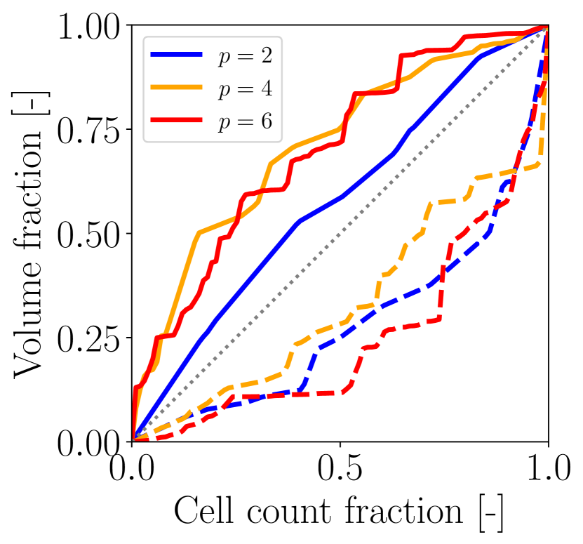
(a) Volume versus cell count.

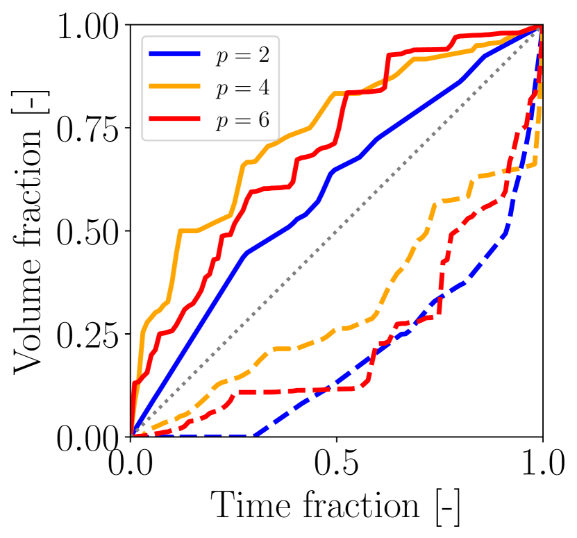
(b) Volume versus runtime.

Figure 1: Normalized convergence plots. Cumulative closed volume, cumulative closed leaf count and runtime are normalized by their final respective values. The solid/dashed lines show the envelope max/min while the dotted reference line shows linear convergence.

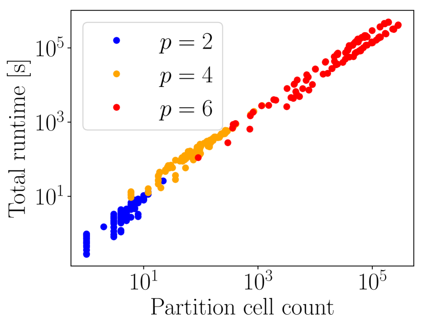
(a) Total runtime statistics.

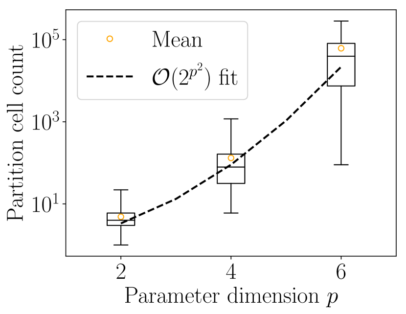
(b) Cell count statistics.

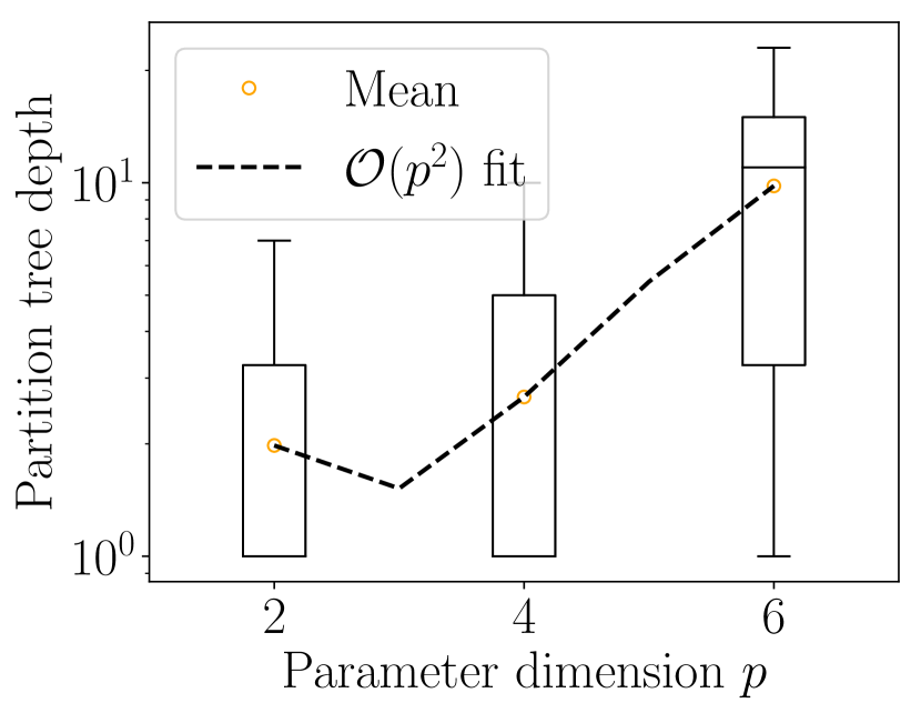
(c) Tree depth statistics.

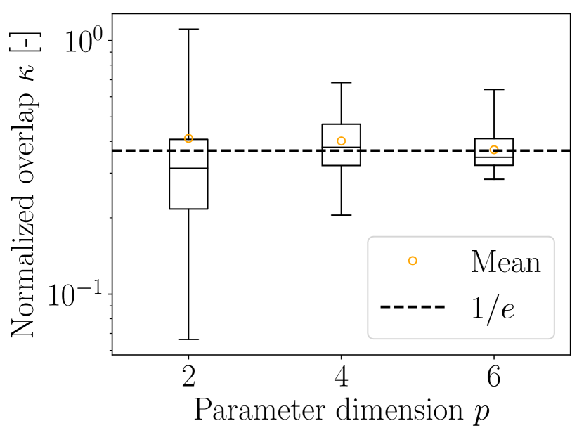
(d) Normalized overlap statistics.

Figure 2: Final partition statistics. Whiskers show the full range.

Figure 1 shows convergence plots using the fraction of the volume of $\Theta$ made up by the closed leafs as the metric. Since at first none and in the end all leaves are closed, this metric goes from $0$ at the start to $1$ at the end of Algorithm 2 and is easily evaluated since the volume of a simplex is well known [34]. The algorithm has a favorable convergence characteristic in that no convergence curve in our tests deviated significantly from a linear rate. The practical significance of this is that the algorithm progresses steadily towards filling up the entire volume of $\Theta$ rather than being very slow at the beginning and very fast at the end or vice versa. Both cases would be poor for the user to supervise since, especially for $p>3$, it becomes difficult to diagnose the reason for slow convergence.

Figure 2(a) shows the wall-clock total runtime corresponding to each run, which appears to increase linearly and with unity slope as a function of the final partition cell count. The linear trend agrees with the linear output complexity of Lemma 3 while the unity slope may be interpreted as that, regardless of $p$, it takes the current implementation on average 1 second to add 1 closed leaf to the partition tree. Note that this measurement includes the time taken to traverse potentially many layers of the tree until adding a closed leaf (up to about 20 layers according to Figure 2(c)). The fact that $p=2,4,6$ all lie on the same trend line indicates that the current implementation’s bottleneck is not the complexity of the intermediate MINLPs that have to be solve but rather e.g. database access speed.

Figures 2(b), 2(c) and 2(d) show statistics on the final tree leaf count and depth along with fitted complexity curves resulting from Section IV-B. Figure 2(b) shows clearly that the partition tree leaf count increases exponentially with $p$ as stipulated by Corollary 2. Interestingly, we note from Figure 2(c) that for some instances of (9) the tree depth does not go beyond the first layer. In other words, sometimes the Delaunay triangulation of $\Theta$ on line 2 of Algorithm 2 suffices. Note that because the complexities in Theorem 2 and Corollary 2 depend also on the overlap $\kappa$, which currently cannot be computed a priori, the regressions in Figures 2(b) and 2(c) carry an omitted variable bias. However, Corollary 2 allows to compute normalized values for $\kappa$ by assuming that the deviations in Figure 2(b) of the actual cell count from the fitted one are due to $\kappa$ alone. This effectively captures the normalized variation required from $\kappa$ in order to explain the deviation of observed results from the regressed theoretical values. This is shown in Figure 2(d) where $\kappa=1/e$ if the match between the fitted and predicted cell counts is perfect. As expected, the effect of $\kappa$ diminishes for higher $p$ where the exponential complexity in $p$ dominates over the polynomial complexity in $\kappa$.

VI Future Work

Algorithm 2 is subject to several potential improvements. First, it would be interesting to compute the overlap $\kappa$ given $\Theta$ and (P_θ). This way, Algorithm 2 could be certified to converge a priori. Next, the partitioning process is parallelizable since lines 5-16 can be executed in parallel for different leafs. Assuming that database communication latency can be highly optimized to the point of being negligible, we can say that lines 5-16 can be made to execute entirely in parallel. Amdahl’s law then predicts that $t_{\mathrm{p}}=t_{\mathrm{s}}/n_{\text{proc}}$ where $t_{\mathrm{p}}$, $t_{\mathrm{s}}$ and $n_{\text{proc}}$ are the parallel total runtime, serial total runtime and number of processors used respectively. The total runtime can thus be reduced in inverse proportion to the number of processors available. Given that modern university facilities can typically provide access to on the order of $10^{2}$ processors and that another $10^{2}$ factor can be achieved by using a compiled programming language, we expect that a compiled parallel implementation can yield a speedup of at least $10^{4}$. According to Figure 2(a), this means that one could compute partitions with $p=4$ in 0.1 s, with $p=6$ in 10 s and (extrapolating) with $p=8$ in 1000 s.

VII Conclusion

This paper presented an algorithm for generating a feasible parameter set partition applicable to hybrid MPC problems. The algorithm consists of systematically breaking down the feasible parameter set into smaller simplices until these can be assigned an integer solution that is feasible everywhere in them. Convergence in a finite number of iterations was proven with novel insight into an overlap characteristic of the MINLP. The on-line evaluation of the partition is polynomial time and thus can be used as a guaranteed real-time warm start of a mixed-integer solver. Extensive testing on randomly generated systems confirmed the complexity calculations, showed favorable convergence properties and suggests that the algorithm is robust enough to be applied on a wide variety of hybrid MPC problems.

VIII Acknowledgment

Part of the research was carried out at the Jet Propulsion Laboratory, California Institute of Technology, under a contract with the National Aeronautics and Space Administration. Government sponsorship acknowledged. The authors would like to extend special gratitude to Daniel P. Scharf, Jack Aldritch and Carl Seubert for their helpful insight and discussions.

References

- [1] D. Mayne, J. Rawlings, C. Rao, and P. Scokaert, “Constrained model predictive control: Stability and optimality,” Automatica, vol. 36, pp. 789–814, jun 2000.
- [2] A. Bemporad and M. Morari, “Robust model predictive control: A survey,” in Robustness in identification and control, pp. 207–226, Springer London, 2007.
- [3] D. Q. Mayne, “Model predictive control: Recent developments and future promise,” Automatica, vol. 50, pp. 2967–2986, dec 2014.
- [4] A. Bemporad and M. Morari, “Control of systems integrating logic, dynamics, and constraints,” Automatica, vol. 35, pp. 407–427, mar 1999.
- [5] C. Ocampo-Martinez, A. Bemporad, A. Ingimundarson, and V. P. Cayuela, “On hybrid model predictive control of sewer networks,” in Identification and Control: the gap between theory and practice (R. Sánchez-Peña, V. Puig, and J. Quevedo, eds.), pp. 87–114, Springer London, 2007.
- [6] L. Blackmore, B. Açıkmeşe, and J. M. Carson, “Lossless convexification of control constraints for a class of nonlinear optimal control problems,” Systems & Control Letters, vol. 61, pp. 863–870, aug 2012.
- [7] T. Schouwenaars, Safe trajectory planning of autonomous vehicles. Dissertation (Ph.D.), Massachusetts Institute of Technology, 2006.
- [8] D. Malyuta, B. Açıkmeşe, and M. Cacan, “Min-max model predictive control for constrained linear systems with state and input dependent uncertainties,” in 2019 American Control Conference (submitted), IEEE, jun 2019.
- [9] A. Richards and J. How, “Model predictive control of vehicle maneuvers with guaranteed completion time and robust feasibility,” in Proceedings of the 2003 American Control Conference, 2003, IEEE, 2003.
- [10] T. S. Hené, V. Dua, and E. N. Pistikopoulos, “A hybrid parametric/stochastic programming approach for mixed-integer nonlinear problems under uncertainty,” Industrial & Engineering Chemistry Research, vol. 41, pp. 67–77, jan 2002.
- [11] D. Corona, I. Necoara, B. D. Schutter, and T. van den Boom, “Robust hybrid MPC applied to the design of an adaptive cruise controller for a road vehicle,” in Proceedings of the 45th IEEE Conference on Decision and Control, IEEE, 2006.
- [12] A. Alessio and A. Bemporad, “A survey on explicit model predictive control,” in Nonlinear Model Predictive Control, pp. 345–369, Springer Berlin Heidelberg, 2009.
- [13] A. Bemporad, “Model predictive control design: New trends and tools,” in Proceedings of the 45th IEEE Conference on Decision and Control, IEEE, 2006.
- [14] E. N. Pistikopoulos, L. Dominguez, C. Panos, K. Kouramas, and A. Chinchuluun, “Theoretical and algorithmic advances in multi-parametric programming and control,” Computational Management Science, vol. 9, pp. 183–203, apr 2012.
- [15] A. Bemporad and C. Filippi, “An algorithm for approximate multiparametric convex programming,” Computational Optimization and Applications, vol. 35, pp. 87–108, mar 2006.
- [16] E. N. Pistikopoulos, M. C. Georgiadis, and V. Dua, eds., Multi‐Parametric Programming: Volume 1: Theory, Algorithms, and Applications, Volume 1, vol. 1. Wiley-VCH Verlag GmbH & Co. KGaA, feb 2007.
- [17] R. H. Oberdieck, Theoretical and algorithmic advances in multi-parametric programming and control. Dissertation (Ph.D.), Imperial College London, 2017.
- [18] M. de la Pena, A. Bemporad, and C. Filippi, “Robust explicit MPC based on approximate multi-parametric convex programming,” in 2004 43rd IEEE Conference on Decision and Control (CDC) (IEEE Cat. No.04CH37601), IEEE, 2004.
- [19] D. M. D. L. Pena, A. Bemporad, and C. Filippi, “Robust explicit MPC based on approximate multiparametric convex programming,” IEEE Transactions on Automatic Control, vol. 51, pp. 1399–1403, aug 2006.
- [20] T. A. Johansen, “Approximate explicit receding horizon control of constrained nonlinear systems,” Automatica, vol. 40, pp. 293–300, feb 2004.
- [21] A. Alessio and A. Bemporad, “Feasible mode enumeration and cost comparison for explicit quadratic model predictive control of hybrid systems,” IFAC Proceedings Volumes, vol. 39, no. 5, pp. 302–308, 2006.
- [22] V. Dua and E. Pistikopoulos, “An outer-approximation algorithm for the solution of multiparametric MINLP problems,” Computers & Chemical Engineering, vol. 22, pp. S955–S958, mar 1998.
- [23] C. Rowe and J. Maciejowski, “An algorithm for multiparametric mixed integer semidefinite optimization,” in 42nd IEEE International Conference on Decision and Control (IEEE Cat. No.03CH37475), IEEE, 2003.
- [24] A. Ingimundarson, C. Ocampo-Martinez, and A. Bemporad, “Suboptimal model predictive control of hybrid systems based on mode-switching constraints,” in 2007 46th IEEE Conference on Decision and Control, IEEE, 2007.
- [25] A. Domahidi, E. Chu, and S. Boyd, “ECOS: An SOCP solver for embedded systems,” in 2013 European Control Conference (ECC), IEEE, jul 2013.
- [26] S. Boyd and L. Vandenberghe, Convex Optimization. Cambridge University Press, 2004.
- [27] D. Dueri, S. V. Rakovic, and B. Acikmese, “Consistently improving approximations for constrained controllability and reachability,” in 2016 European Control Conference (ECC), IEEE, jun 2016.
- [28] M. Baotić, “Polytopic computations in constrained optimal control,,” Automatika, Journal for Control, Measurement, Electronics, Computing and Communications, vol. 50, pp. 119–134, 2009.
- [29] M. de Berg, M. van Kreveld, M. Overmars, and O. Schwarzkopf, Computational Geometry. Springer Berlin Heidelberg, 3 ed., 2008.
- [30] A. S. Phani, “On the necessary and sufficient conditions for the existence of classical normal modes in damped linear dynamic systems,” Journal of Sound and Vibration, vol. 264, pp. 741–745, jul 2003.
- [31] P. J. Antsaklis and A. N. Michel, A Linear Systems Primer. Birkhäuser Boston, 2007.
- [32] J.-C. Hennet, “Discrete time constrained linear systems,” in Control and Dynamic Systems, pp. 157–213, Elsevier, 1995.
- [33] P. Trodden, “A one-step approach to computing a polytopic robust positively invariant set,” IEEE Transactions on Automatic Control, vol. 61, pp. 4100–4105, dec 2016.
- [34] P. Stein, “A note on the volume of a simplex,” The American Mathematical Monthly, vol. 73, p. 299, mar 1966.