Robust Model Predictive Control for Linear Systems with State and Input Dependent Uncertainties

Abstract

This paper presents a computationally efficient robust model predictive control law for discrete linear time invariant systems subject to additive disturbances that may depend on the state and/or input norms. Despite the dependency being non-convex, we are able to handle it as a second-order cone program. Both open-loop and semi-feedback planning strategies are presented. The formulation has linear complexity in the planning horizon length. The approach is thus amenable to efficient real-time implementation with a guarantee on recursive feasibility and global optimality. Robust position control of a satellite is considered as an illustrative example.

I Introduction

In this paper we develop a novel convex formulation for robust model predictive control (RMPC) of discrete linear time invariant systems with additive state and/or input dependent uncertainty. A major advantage of RMPC is its ability to guarantee by design that input and state constraints are satisfied for all uncertainty realizations. Several extensive survey papers cover available modeling assumptions and solution methods [4, 5]. We restrict our attention to discrete linear time invariant systems and focus on developing a real-time implementable algorithm on computationally constrained hardware. We assume a perfect dynamics model affected by additive bounded uncertainty and present open-loop and semi-feedback planning strategies [4, Section 8]. Note that these strategies merely refer to the method of handling uncertainty within the RMPC optimization problem. In each case, the on-line implementation is done in the traditional feedback sense of re-solving and applying the first of the optimal control inputs at every time step. Several authors have considered closed-loop formulations [6, 7, 8, 9, 10]. However, these suffer from combinatorial complexity in the problem dimension unless certain restrictive assumptions are made in terms of cost norm or feedback type.

Closest to our work [11, 12, 13] and [14] use pre-computed constraint tightening factors to guarantee robustness to worst-case uncertainty through a set of linear constraints. The computational cost is marginally higher than that of nominal MPC and the online problem is at most a quadratic program (QP). A similar idea is exploited for nonlinear systems in [15]. Dependent uncertainty has received some attention in nonlinear MPC [16, 17, 18]. These formulations, however, are conservative due to their use of a Lipschitz constant for constraint tightening, which considers uncertainty magnitude but not direction The incrementally conic uncertainty model in [19] is used to assure robustness via a static feedback component obtained by an off-line linear matrix inequality procedure and an on-line nominal MPC law, as in tube MPC [20].

Our main contribution is to present how a state and input dependent uncertainty model can be included in RMPC while retaining low computational complexity. We present an open-loop formulation first and, because it can be overly conservative, extend it to a semi-feedback formulation where a static feedback gain is embedded into the planning task [7, 21]. Our model is a subset of [19] but has the advantage of using the more computationally efficient second-order cone programming (SOCP) for a robust solution. Furthermore, unlike [16, 17, 18], our method captures disturbance directionality effects via Hölder’s inequality and is therefore less conservative. Finally, we illustrate how the uncertainty model can describe the very popular Gates thruster execution-error model for satellites [1, 2, 22]. Because our approach has linear complexity in the horizon length and is at most an SOCP problem, we expect the algorithm to be amenable to real-time implementation [23, 24, 25, 26].

The paper is organized as follows. In Section II the uncertainty model and the resulting robust optimal control problem are introduced. In Section III a solution is presented as an open-loop RMPC law that is at most an SOCP problem. Section IV proves recursive feasibility and suggests a computationally efficient check of robust controlled invariance. Section V converts the formulation to a semi-feedback implementation. An example is presented in Section VI which illustrates the method’s effectiveness. Section VII discusses possible extensions and offers concluding remarks.

Notation: $\mathbb{R}$, $\mathbb{R}_{+}$ and $\mathbb{R}_{++}$ are the reals, non-negative reals and positive reals. Unless otherwise specified, matrices are uppercase (e.g. $A$), scalars and vectors are lowercase (e.g. $x$) and sets are calligraphic uppercase (e.g. $\mathcal{S}$). $0_{n\times m}\in\mathbb{R}^{n\times m}$ and $I_{n}\in\mathbb{R}^{n\times n}$ are the zero and identity matrices respectively, where $n=m=3$ when the subscripts are omitted. Parentheses denote vertical stacking, e.g. $(1,2,3)\in\mathbb{R}^{3}$. $M_{i}^{\scriptscriptstyle\mathsf{T}}$ denotes the $i$-th row of matrix $M$. $\|\cdot\|_{p}$ denotes the $p$-norm, e.g. $p=1,2,\infty$. ${\mathop{\mathrm{missing}}{co}}\mathcal{S}$ is the convex hull of $\mathcal{S}$. Direct set mapping is written as $M\mathcal{S}=\{Mx:x\in\mathcal{S}\}$. The support function of $\mathcal{S}\subseteq\mathbb{R}^{n}$ along a direction $v\in\mathbb{R}^{n}$ is denoted $\sigma_{\mathcal{S}}(v)\triangleq\max_{z\in\mathcal{S}}v^{\scriptscriptstyle\mathsf{T}}z$. The shorthand $a:b$ represents the integer sequence $a,\dots,b$. $\mathcal{S}^{a}$ is the Cartesian product performed $a$ times, e.g. $\mathcal{S}^{3}=\mathcal{S}\times\mathcal{S}\times\mathcal{S}$.

II Problem Formulation

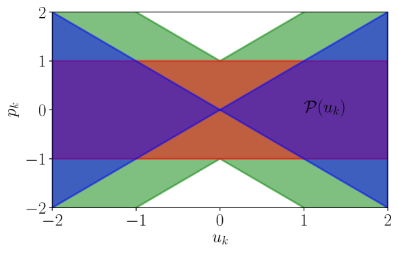
Figure 1: Non-convex input dependent uncertainty set $\mathcal{P}(u_{k})$ (green), expressed as the Minkowski sum of a polytopic independent component (red) and a conic dependent component (blue).

This section describes the control problem and, in particular, defines the state and input dependent uncertainty model. Consider a discrete linear time invariant system with additive uncertainty:

$$x_{k+1}=Ax_{k}+Bu_{k}+Dp_{k},$$ (1)

where $k\in\mathbb{Z}_{+}$, $x_{k}\in\mathbb{R}^{n}$, $u_{k}\in\mathbb{R}^{m}$ and $p_{k}\in\mathbb{R}^{d}$ are, respectively, the time step, state, input and uncertainty, while $A$, $B$ and $D$ are constant matrices of commensurate dimension. The following state and input constraints are to be respected for all time:

$$x_{k} \in\mathcal{X}\subset\mathbb{R}^{n}\quad \forall k\in\mathbb{Z}_{+},$$ (2a)

$$u_{k} \in\mathcal{U}\subset\mathbb{R}^{m}\quad \forall k\in\mathbb{Z}_{+},$$ (2b)

where $\mathcal{X}$ and $\mathcal{U}$ are compact convex polytopes that we express as follows:

$$\mathcal{X} \triangleq\{x\in\mathbb{R}^{n}:Fx\leq f\},$$ (3a)

$$\mathcal{U} \triangleq\{u\in\mathbb{R}^{m}:Hu\leq h\},$$ (3b)

where the rows of $F$, $H$ and the elements of $f$, $h$ define respectively the polytope facet normals and distances. Consider now the following uncertainty model:

$$p_{k} \in\mathcal{P} (x_{k},u_{k})\subset\mathbb{R}^{d},$$ (4a)

$$\mathcal{P}(x_{k},u_{k}) \triangleq\{ Ww+\sum_{i=1}^{n_{q}}L_{i}q_{i}\in\mathbb{R}^{d}:Rw\leq r,$$ (4b)

$$\|q_{i}\|_{p_{q,i}}\leq\phi_{i}(\|F_{x,i}x_{k}\|_{p_{x,i}},\|F_{u,i}u_{k}\|_{p_{u,i}}),$$

$$i=1,\dots,n_{q}\},$$

where each function $\phi_{i}:\mathbb{R}_{+}\times\mathbb{R}_{+}\to\mathbb{R}_{+}$ is convex and non-decreasing such that $\phi_{i}(\|\cdot\|_{p_{x,i}},\|\cdot\|_{p_{u,i}})$ is convex [27]. The uncertainty set is effectively the sum of an independent component originating from a polytope and a state and input dependent component that is bounded by a non-convex inequality. Because unbounded disturbances are not practical, we assume that $\mathcal{P}(x_{k},u_{k})$ is compact $\forall x_{k}\in\mathcal{X},~{}u_{k}\in\mathcal{U}$. Note that $\mathcal{P}(x_{k},u_{k})$ is a non-convex set. A simple example of (4b) for $n=m=d=n_{q}=1$ and no state dependency is illustrated in Figure 1, where:

$$W=1,\,\,R=\begin{bmatrix}1\\ -1\end{bmatrix},\,\,r=\begin{bmatrix}1\\ 1\end{bmatrix},\,\,L_{1}=1,\,\,\phi_{1}(|u_{k}|)=|u_{k}|.$$

Summarizing, the control problem is to chose an input $u_{k}$ at each time $k\in\mathbb{Z}_{+}$ such that given $x_{0}\in\mathcal{X}$ and the system dynamics (1), the constraints (2a) and (2b) are satisfied subject to any uncertainty specified by (4a). We assume that the control objective to be minimized can be expressed as a convex function of $x_{k}$ and $u_{k}$.

III Control Law Description

In this section we develop an RMPC law with a planning horizon of length $N\in\mathbb{Z}_{++}$ that solves the control problem presented in Section II. We begin with a set theoretic motivation for how the state constraint (2a) may be robustly satisfied given the input constraint (2b) and the uncertainty (4a).

Definition 1.

A compact convex set $\mathcal{I}$ is feasible robust controlled invariant (fRCI) for system (1) and constraints (2a), (2b) and (4a) if it satisfies the following definition:

$$\mathcal{I}=\{x\in\mathcal{X}:\exists u\in\mathcal{U}\text{ s.t. }Ax+Bu+Dp\in\mathcal{I}\,\,\forall p\in\mathcal{P}(x,u)\}.$$

By constraining $x_{k}\in\mathcal{I}\subseteq\mathcal{X}$, the state constraint can thus be feasibly satisfied for all time as long as $x_{0}\in\mathcal{I}$. Numerous set-based iterative methods are available for computing the maximal volume $\mathcal{I}$ [28, 29, 30]. Approaches like [30] that attempt to deal with state and input dependent uncertainty, however, scale poorly beyond $n=2$ because they require computing set differences and projections of polytopes. Both operations have $\mathcal{O}(2^{n})$ complexity [31]. For this reason we use a more computationally efficient algorithm developed for independent uncertainty and which avoids these two operations [29]. This requires using the convex hull of our uncertainty model:

$$p_{k}\in{\mathop{\mathrm{missing}}{co}}\{\mathcal{P}(x_{k},u_{k}):x_{k}\in\mathcal{X},\,u_{k}\in\mathcal{U}\}.$$ (5)

While this introduces conservatism into the computation of $\mathcal{I}$ by considering a larger uncertainty set, the approach is more scalable to higher dimensions given existing methods for computing fRCI sets. Furthermore, Corollary 1 in Section IV presents a computationally efficient method for checking if $\mathcal{X}$ itself is fRCI, at which point the computation of $\mathcal{I}$ can be avoided altogether as described in Algorithm 1. The proof of Theorem 1 in Section IV shows that $\mathcal{I}$ is a convex set and may therefore be inner-approximated by a polytope. We henceforth assume that this polytopic description is available:

$$\mathcal{I}\triangleq\{x\in\mathbb{R}^{n}:Gx\leq g\},$$ (6)

where $G\in\mathbb{R}^{n_{g}\times n}$ and $g\in\mathbb{R}^{n_{g}}$.

Since $\mathcal{I}$ is fRCI, for each $x_{k}\in\mathcal{I}$ $\exists u_{k}\in\mathcal{U}$ such that $x_{k+1}\in\mathcal{I}$ $\forall p_{k}\in\mathcal{P}(x_{k},u_{k})$. We compute such a $u_{k}$ via a tightened state constraint in an optimization problem. Letting $x_{k}$ be the current state, the system (1) has the following impulse response over $t=1:N$ future time steps:

$$x_{k+t}=A^{t}x_{k}+\sum_{i=0}^{t-1}B^{A}_{i}u_{k+i}+\sum_{i=0}^{t-1}D^{A}_{i}p_{k+i},$$ (7)

where $B^{A}_{i}\triangleq A^{t-1-i}B$ and $D^{A}_{i}\triangleq A^{t-1-i}D$ (the index $t$ is omitted for notational simplicity). An invariance-preserving input sequence over the $N$-step planning horizon satisfies:

$$G\left(A^{t}x_{k}+\sum_{i=0}^{t-1}B^{A}_{i}u_{k+i}+\sum_{i=0}^{t-1}D^{A}_{i}p_{k+i}\right)\leq g,$$ (8)

for all sequences $p_{k+i}\in\mathcal{P}(x_{k+i},u_{k+i})$, $i=0:t-1$ and $t=1:N$. Similarly to [11, 32] we reformulate this requirement by maximizing the left hand side of (8):

$$G_{j}^{\scriptscriptstyle\mathsf{T}}\bar{x}_{k+t}+\sum_{i=0}^{t-1}\max_{p_{k+i}\in\mathcal{P}(x_{k+i},u_{k+i})}G_{j}^{\scriptscriptstyle\mathsf{T}}D^{A}_{i}p_{k+i}\leq g_{j},$$ (9)

for $j=1:n_{g}$ and $t=1:N$, where $\bar{x}_{k+t}$ denotes the nominal state after $t$ time steps:

$$\bar{x}_{k+t}\triangleq A^{t}x_{k}+\sum_{i=0}^{t-1}B^{A}_{i}u_{k+i}.$$ (10)

Note that the maximization term in (9) is the support function $\sigma_{D^{A}_{i}\mathcal{P}(x_{k+i},u_{k+i})}(G_{j})\in\mathbb{R}_{+}$ where $G_{j}$ is $\mathcal{I}$’s $j$-th facet’s normal. This support function induces constraint tightening.

A complication arises in evaluating the support function due to an algebraic loop in the state dependent uncertainty. The set $\mathcal{P}(x_{k+i},u_{k+i})$ depends on $x_{k+i}$ which itself depends on the uncertainty sequence over time steps $0:i-1$ in the planning horizon. Thus, $p_{k+i}$ becomes dependent on $p_{k},\dots,p_{k+i-1}$ and the maximum value that it can take involves the maximization of a convex function over a non-convex domain. Simulation experience with the example in Section VI shows that a convex upper bound to this maximization is too conservative, thus we prefer to simplify by considering instead the uncertainty set $\mathcal{P}(\bar{x}_{k+i},u_{k+i})$ based on the nominal state. While this choice has no impact at $t=1$ (since $x_{k}=\bar{x}_{k}$), the same cannot be said over the remaining $N-1$ steps because perturbed states with a larger norm may occur, inducing a larger uncertainty than the one predicted by $\mathcal{P}(\bar{x}_{k+i},u_{k+i})$. However, since RMPC is implemented in receding horizon fashion and $u_{k}$ is anyway the only input to be applied, the implementation remains robust. Furthermore, note that the formulation remains exact over the entire planning horizon for input dependent uncertainty.With this in mind, the support function in (9) is simplified using the separable nature of (4b) and Hölder’s inequality:

$$\begin{split}&\sigma_{D^{A}_{i}\mathcal{P}(\bar{x}_{k+i},u_{k+i})}(G_{j})=\sigma_{D^{A}_{i}\mathcal{W}}(G_{j})+\\ &\sum_{l=1}^{n_{q}}\|G_{j}^{\scriptscriptstyle\mathsf{T}}D^{A}_{i}L_{l}\|_{q_{q,l}}\phi_{l}(\|F_{x,l}\bar{x}_{k+i}\|_{p_{x,l}},\|F_{u,l}u_{k+i}\|_{p_{u,l}}),\end{split}$$ (11)

where the $q_{q,l}$-norm is dual to the $p_{q,l}$-norm in (4b), i.e. $1/q_{q,l}+1/p_{q,l}=1$, and we denote by $\mathcal{W}\triangleq\{Ww:Rw\leq r\}$ the polytopic independent uncertainty part of $\mathcal{P}(\bar{x}_{k+i},u_{k+i})$. Note that (11) is not conservative since Hölder’s inequality is tight [27]. Using (11), we can write (9) as a set of $Nn_{g}$ convex constraints:

$$\begin{split}&G_{j}^{\scriptscriptstyle\mathsf{T}}\bar{x}_{k+t}+\sum_{i=0}^{t-1}\sigma_{D^{A}_{i}\mathcal{W}}(G_{j})+\\ &\sum_{i=0}^{t-1}\sum_{l=1}^{n_{q}}\|G_{j}^{\scriptscriptstyle\mathsf{T}}D^{A}_{i}L_{l}\|_{q_{q,l}}\phi_{l}(\|F_{x,l}\bar{x}_{k+i}\|_{p_{x,l}},\\ &\hskip 106.69783pt\|F_{u,l}u_{k+i}\|_{q_{u_{l}}})\leq g_{j},\end{split}$$ (12)

for $j=1:n_{g}$ and $t=1:N$. Importantly, $\sigma_{D^{A}_{i}\mathcal{W}}(G_{j})$ can be pre-computed offline leading to a more efficient implementation. The RMPC on-line optimization problem to be implemented in receding horizon fashion can thus be written as:

$$\underset{u_{k},\dots,u_{k+N-1}}{\text{minimize}} J(\bar{x}_{k+1},\dots,\bar{x}_{k+N},u_{k},\dots,u_{k+N-1})$$ (13)

subject to (2b) and (12).

where the cost function $J:(\mathbb{R}^{n})^{N}\times(\mathbb{R}^{m})^{N}\to\mathbb{R}$ is a design choice which should be convex. If $J$ is linear and the 1- or $\infty$-norms are used for all $\phi_{l}$ in (12), this is a linear program (LP). If $J$ is quadratic, it is a QP. In all cases when the 2-norm is used in the $\phi_{l}$ functions, (13) is an SOCP. Note that all of these problem types are convex and have efficient solvers available that guarantee convergence to the global optimum when the feasible set is non-empty (which it is certified to always be in Section IV). Furthermore, the constraint count of (13) is $\mathcal{O}(N)$ owing to the welcome property that the effect of worst-case uncertainty on a discrete time linear system is explicitly given by (11), avoiding a combinatorial search. Algorithm 1 summarizes the off-line and on-line steps that make up the full RMPC controller.

Off-line:

if Corollary 1 is satisfied for $\mathcal{I}=\mathcal{X}$ then

     $\mathcal{I}\leftarrow\mathcal{X}$

else

     Compute $\mathcal{I}$ using the set-based algorithm in [29]

     if Corollary 1 is not satisfied for $\mathcal{I}$ then

         Report error “$N$ is too large”      

Store $\sigma_{D^{A}_{i}\mathcal{W}}(G_{j})$ for $j=1:n_{g}$, $t=1:N$, $i=0:t-1$

On-line:

Obtain the current state $x$

Set $x_{k}\leftarrow x$, solve (13) and apply $u_{k}$

Sleep $T_{\text{s}}$ seconds$\triangleright$ Discretization time step

Algorithm 1 Off-line and on-line RMPC steps.

IV Main Results

In this section, Theorem 1 proves that the control law (13) is recursively feasible and Corollary 1 provides an alternative sufficient condition for certifying $\mathcal{X}$ to be fRCI. This helps to avoid laborious set-based approaches for computing $\mathcal{I}$.

Theorem 1.

The optimization problem (13) is recursively feasible if and only if it is feasible at the vertices of $\mathcal{I}$.

Proof.

Let $\mathcal{V}\triangleq\{v_{1},...,v_{M}\}$ be the set of vertices of $\mathcal{I}$. The forward implication is trivial. If (13) is recursively feasible then it is feasible in particular when $x_{k}\in\mathcal{V}$. For the reverse implication, suppose that we solve (13) with $x_{k}$ set to each vertex $v_{m}$, $m=1:M$, and obtain associated optimal input sequences $u_{k+t}^{m}$, $t=0:N-1$, and nominal state sequences $\bar{x}_{k+t}^{m}$, $t=0:N$, as given by (10):

$$\bar{x}_{k+t}^{m}=A^{t}v_{m}+\sum_{i=0}^{t-1}B^{A}_{i}u_{k+i}^{m}.$$

Consider now a state $x_{k}\in\mathcal{I}$. Since $\mathcal{I}$ is a convex polytope, we can express $x_{k}$ as a convex combination of $\mathcal{I}$’s vertices:

$$x_{k}=\sum_{m=1}^{M}\theta_{m}v_{m},\,\sum_{m=1}^{M}\theta_{m}=1,\,\theta_{m}\geq 0\,\,\forall m=1:M.$$

It is now possible to sum the constraint (12) applied at each vertex, weighted by $\theta_{m}$, to obtain:

$$\begin{split}&G_{j}^{\scriptscriptstyle\mathsf{T}}\sum_{m=1}^{M}\theta_{m}\bar{x}_{k+t}^{m}+\sum_{i=0}^{t-1}\sigma_{D^{A}_{i}\mathcal{W}}(G_{j})+\\ &\sum_{i=0}^{t-1}\sum_{l=1}^{n_{q}}\|G_{j}^{\scriptscriptstyle\mathsf{T}}D^{A}_{i}L_{l}\|_{q_{q,l}}\sum_{m=1}^{M}\theta_{m}\phi_{l}(\|F_{x,l}\bar{x}_{k+i}^{m}\|_{p_{x,l}},\\ &\hskip 136.57323pt\|F_{u,l}u_{k+i}^{m}\|_{p_{u,l}})\leq g_{j}.\end{split}$$

Because each $\phi_{l}$ is convex, it follows from Jensen’s inequality that:

$$\begin{split}\phi_{l}(\|F_{x,l}&\sum_{m=1}^{M}\theta_{m}\bar{x}_{k+i}^{m}\|_{p_{x,l}},\|F_{u,l}\sum_{m=1}^{M}\theta_{m}u_{k+i}^{m}\|_{p_{u,l}})\leq\\ &\sum_{m=1}^{M}\theta_{m}\phi_{l}(\|F_{x,l}\bar{x}_{k+i}^{m}\|_{p_{x,l}},\|F_{u,l}u_{k+i}^{m}\|_{p_{u,l}}),\end{split}$$

and as a result we have:

$$\begin{split}&G_{j}^{\scriptscriptstyle\mathsf{T}}\sum_{m=1}^{M}\theta_{m}\bar{x}_{k+t}^{m}+\sum_{i=0}^{t-1}\sigma_{D^{A}_{i}\mathcal{W}}(G_{j})+\\ &\sum_{i=0}^{t-1}\sum_{l=1}^{n_{q}}\|G_{j}^{\scriptscriptstyle\mathsf{T}}D^{A}_{i}L_{l}\|_{q_{q,l}}\phi_{l}(\|F_{x,l}\sum_{m=1}^{M}\theta_{m}\bar{x}_{k+i}^{m}\|_{p_{x,l}},\\ &\|F_{u,l}\sum_{m=1}^{M}\theta_{m}u_{k+i}^{m}\|_{p_{u,l}})\leq g_{j}.\end{split}$$ (14)

Because $\mathcal{U}$ is convex and $u_{k+i}^{m}\in\mathcal{U}$ $\forall m=1:M$, $i=0:N-1$, we have $\sum_{m=1}^{M}\theta_{m}u_{k+i}^{m}\in\mathcal{U}$ $\forall i=0:N-1$. Furthermore:

$$\sum_{m=1}^{M}\theta_{m}\bar{x}_{k+t}^{m}=A^{t}x_{k}+\sum_{i=0}^{t-1}B^{A}_{i}\sum_{m=1}^{M}\theta_{m}u_{k+i}^{m}.$$

We thus recognize that (14) is nothing but (12) for the initial state $x_{k}$ and the feasible input sequence $\sum_{m=1}^{M}\theta_{m}u_{k+i}^{m}$, $i=0:N-1$. The feasible set of (13) is thus non-empty. Since this control input ensures that $x_{k+1}\in\mathcal{I}$ under the worst-case disturbance, (13) continues to be feasible at the next time step which means that it is recursively feasible. ∎

The following corollary provides a more computationally efficient method than computational geometry approaches for verifying that a particular polytope is fRCI. This is used in Algorithm 1 for checking if $\mathcal{X}$ in (2a) is fRCI, avoiding an unnecessary call to the more time consuming set-based algorithm in [29], especially for high dimensional systems.

Corollary 1.

Let $\mathcal{I}=\mathcal{X}$. A sufficient condition for $\mathcal{I}$ to be fRCI is for (13) to be feasible at its vertices. The condition becomes also necessary when $N=1$.

Proof.

The sufficient condition follows from Theorem 1 and the fact that (12) yields the fRCI property by design whenever (13) is recursively feasible. The necessity of this condition when $N=1$ is a consequence of that no conservatism in the planning problem is then present. ∎

V Extension to Semi-feedback RMPC

The open-loop RMPC law (13) can be overly conservative because it does not model feedback action, meaning that the open-loop control policy $\{u_{k},\dots,u_{k+N-1}\}$ cannot mitigate the effect of disturbances during the planning stage [4]. Indeed, the disturbance action terms $\sigma_{D_{i}^{A}\mathcal{W}}(G_{j})$ and $\|G_{j}^{\scriptscriptstyle\mathsf{T}}D_{i}^{A}L_{l}\|_{q_{q,l}}$ in (12) are independent of the control policy. This section extends our formulation to semi-feedback RMPC [7, 21] which introduces feedback action into the planning stage without significantly increasing computational complexity. To this end, a static feedback gain $K$ is designed and the control is re-defined as

$$u_{k}=v_{k}+Kx_{k},$$ (15)

such that $v_{k}\in\mathbb{R}^{m}$ becomes the decision variable. The nominal state (10) becomes:

$$\bar{x}_{k+t}=\tilde{A}^{t}x_{k}+\sum_{i=0}^{t-1}B_{i}^{\tilde{A}}v_{k+i},$$ (16)

where $\tilde{A}=A+BK$. The robust constraint (12) becomes:

$$\begin{split}&G_{j}^{\scriptscriptstyle\mathsf{T}}\bar{x}_{k+t}+\sum_{i=0}^{t-1}\sigma_{D^{\tilde{A}}_{i}\mathcal{W}}(G_{j})+\\ &\sum_{i=0}^{t-1}\sum_{l=1}^{n_{q}}\|G_{j}^{\scriptscriptstyle\mathsf{T}}D^{\tilde{A}}_{i}L_{l}\|_{q_{q,l}}\phi_{l}(\|F_{x,l}\bar{x}_{k+i}\|_{p_{x,l}},\\ &\hskip 78.24507pt\|F_{u,l}(v_{k+i}+K\bar{x}_{k+i})\|_{q_{u_{l}}})\leq g_{j},\end{split}$$ (17)

where we have used the nominal state for the input-dependent input error. Applying the discussion in Section III, this choice has no impact at $t=1$ so the RMPC law remains robust when implemented in receding horizon fashion. With these changes, semi-feedback RMPC can be implemented in the same way as (13).

VI Illustrative Example

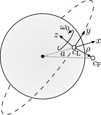
Figure 2: LVLH frame showing the leader and follower satellites.

In this section the control law presented in Sections III and V is applied to satellite robust position control in low Earth orbit. Consider a two satellite formation as shown in Figure 2 with a leader $c_{\text{L}}$ in a circular orbit with radius $a$ and a follower $c_{\text{F}}$. The follower’s translation in a local vertical local horizontal (LVLH) frame is given by the Clohessy-Wiltshire equations (time is omitted for notational simplicity):

$$\ddot{x} =3\omega_{0}^{2}x+2\omega_{0}\dot{y}+u_{x}+w_{x},$$ (18a)

$$\ddot{y} =-2\omega_{0}\dot{x}+u_{y}+w_{y},$$ (18b)

$$\ddot{z} =-\omega_{0}^{2}z+u_{z}+w_{z},$$ (18c)

where $\omega_{0}=\sqrt{\mu/a^{3}}$ and $\mu$ is the standard gravitational parameter. Let $\rho=(x,y,z)\in\mathbb{R}^{3}$ denote the follower’s position relative to the leader, where the coordinate $x$ is not to be confused with the state vector. Using the state $x\triangleq(\rho,\dot{\rho})\in\mathbb{R}^{6}$, input $u=(u_{x},u_{y},u_{z})\in\mathbb{R}^{3}$ and exogenous disturbance $w=(w_{x},w_{y},w_{z})\in\mathbb{R}^{3}$, the dynamics (18a)-(18c) take on the familiar linear form:

$$\dot{x}=A_{\text{c}}x+B_{\text{c}}(u+w).$$ (19)

We use an impulsive control input in which the RCS system can induce an instantaneous velocity increment $\Delta v(\tau)$ at time $\tau$ via the control input $u(t)=\Delta v(\tau)\delta(t-\tau)$, where $\delta$ is the Dirac delta, every $T_{\text{s}}$ seconds. Meanwhile, $w$ is assumed to be a constant acceleration over the $T_{\text{s}}$ period. These assumptions allow (19) to be discretized [33]:

$$x_{k+1}=Ax_{k}+Bu_{k}+Ew_{k},$$ (20)

$$A=e^{A_{\text{c}}T_{\text{s}}},\quad B=AB_{\text{c}},\quad E=\int_{0}^{T_{\text{s}}}e^{A(T_{\text{s}}-t)}B\mathrm{d}t.$$

We include three uncertainty sources:

1. Atmospheric drag, modeled as an independent component $w_{k}\in\{w:\|w\|_{\infty}\leq w_{\max}\}$;

2. Additive input error using the Gates model, which captures the error in the RCS system’s reproduction of a $\Delta v$ desired velocity increment [1, 2, 22]. Because (4b) does not capture directional dependency, we confine ourselves to an isotropic description. In fact this is anyway the best modeling choice if the satellite’s design is unknown [1]. The error term is $v_{k}=v_{k}^{\text{fix}}+v_{k}^{\text{prop}}$ where $v_{k}^{\text{fix}}\in\{v:\|v\|_{2}\leq\sigma_{\text{fix}}\}$ and $v_{k}^{\text{prop}}\in\{v:\|v\|_{2}\leq\sigma_{\text{rcs}}\|u_{k}\|_{2}\}$;

3. Additive state estimation error $e_{k}=e_{k}^{\text{fix}}+(I,0)e_{k}^{\text{pos}}+(0,I)e_{k}^{\text{vel}}$ where:

$$\begin{split}e_{k}^{\text{fix}}&\in\{e\in\mathbb{R}^{6}:\|\begin{bmatrix}I&0\end{bmatrix}e\|_{\infty}\leq p_{\max},\|\begin{bmatrix}0&I\end{bmatrix}e\|_{\infty}\leq v_{\max}\},\\ e_{k}^{\text{pos}}&\in\{e\in\mathbb{R}^{3}:\|e\|_{\infty}\leq\sigma_{\text{pos}}\|\begin{bmatrix}I&0\end{bmatrix}x_{k}\|_{2}\},\\ e_{k}^{\text{vel}}&\in\{e\in\mathbb{R}^{3}:\|e\|_{\infty}\leq\sigma_{\text{vel}}\|\begin{bmatrix}0&I\end{bmatrix}x_{k}\|_{2}\}.\end{split}$$

Altogether, these form a set of independent and dependent polytopic and ellipsoidal uncertainties that is readily described by (4b). In particular, $d=21$, $n_{q}=4$, $w=(w_{k},e_{k}^{\text{fix}})$, $q_{1}=v_{k}^{\text{fix}}$, $q_{2}=v_{k}^{\text{prop}}$, $q_{3}=e_{k}^{\text{pos}}$, $q_{4}=e_{k}^{\text{vel}}$, $p_{q,1}=p_{q,2}=2$, $p_{q,3}=p_{q,4}=\infty$, $\phi_{1}=\sigma_{\text{fix}}$, $\phi_{2}:u_{k}\mapsto\sigma_{\text{rcs}}\|u_{k}\|_{2}$, $\phi_{3}:x_{k}\mapsto\sigma_{\text{pos}}\|\begin{bmatrix}I&0\end{bmatrix}x_{k}\|_{2}$, $\phi_{4}:x_{k}\mapsto\sigma_{\text{vel}}\|\begin{bmatrix}0&I\end{bmatrix}x_{k}\|_{2}$ and the following matrices:

$$D=\begin{bmatrix}E&-A&B&B&-A&-A\end{bmatrix}$$

$$W=(I_{9},0_{18\times 9})\,\,\,\,R=(I_{9},-I_{9})$$

$$r=(w_{\max}\bm{1},p_{\max}\bm{1},v_{\max}\bm{1},w_{\max}\bm{1},p_{\max}\bm{1},v_{\max}\bm{1})$$

$$L_{1}=(0_{9\times 3},I,0_{15\times 3})\,\,\,\,L_{2}=(0_{12\times 3},I,0_{12\times 3})$$

$$L_{3}=(0_{15\times 3},I,0_{9\times 3})\,\,\,\,L_{4}=(0_{24\times 3},I),$$

where $\bm{1}\in\mathbb{R}^{3}$ is a vector of ones. We use the following cost:

$$J\triangleq\sum_{t=0}^{N-1}\hat{u}_{k+t}^{\scriptscriptstyle\mathsf{T}}\hat{u}_{k+t}+\lambda\hat{\bar{x}}_{k+t+1}^{\scriptscriptstyle\mathsf{T}}\hat{\bar{x}}_{k+t+1},$$ (21)

where $\hat{u}_{k+t}$ and $\hat{\bar{x}}_{k+t+1}$ are the scaled input and nominal state such that they attain plus or minus unity at the boundary of their respective constraint polytopes $\mathcal{U}$ and $\mathcal{I}$ while $\lambda=0.003$ is a manually chosen trade-off weight. The input penalty reflects a minimum-fuel type problem and the state penalty endows the finite horizon control law with an otherwise lacking long-term knowledge that the origin corresponds to minimal fuel usage, since nominally it takes zero control action to remain there. In this problem, $\mathcal{X}$ in (2a) takes on the direct interpretation of a maximum control error specification. We use the following numerical values:

$$\mathcal{X}=\{x\in\mathbb{R}^{6}:\|\begin{bmatrix}I&0\end{bmatrix}x\|_{\infty}\leq 10\text{ cm},\|\begin{bmatrix}0&I\end{bmatrix}x\|_{\infty}\leq 1\text{ mm/s}\}$$

$$\mathcal{U}=\{u\in\mathbb{R}^{3}:\|u\|_{\infty}\leq 2\text{ mm/s}\}$$

$$\mu=3.986\cdot 10^{14}\text{ m}^{3}\text{/s}^{2}\,\,\,a=6793.137\text{ km}\,\,\,T_{\text{s}}=100\text{ s}$$

$$w_{\max}=50\text{ nm/s}^{2}\,\,\,\sigma_{\text{fix}}=1\text{ }\mu\text{m/s}\,\,\,p_{\max}=0.4\text{ cm}\,\,\,N=4$$

$$v_{\max}=4\text{ }\mu\text{m/s}\,\,\,\sigma_{\text{rcs}}=\tan\frac{\pi}{180}\,\,\,\sigma_{\text{pos}}=0.02\,\,\,\sigma_{\text{vel}}=0.001.$$

We compare the following four controllers:

1. Nominal MPC: ignores the uncertainty, effectively removing the summations in (12);

2. Conservative RMPC: replaces $\phi_{i}$ in (4b) by its maximum over $x_{k}\in\mathcal{X}$ and $u_{k}\in\mathcal{U}$, which results in a conservative independent uncertainty model;

3. Our open-loop RMPC law (13);

4. Our semi-feedback RMPC law using the modifications described in Section V. We design $K$ via LQR with weight matrices $Q=I_{6}$ and $R=10^{5}I$, scaled to $\mathcal{I}$ and $\mathcal{U}$ respectively in the same way as for (21).

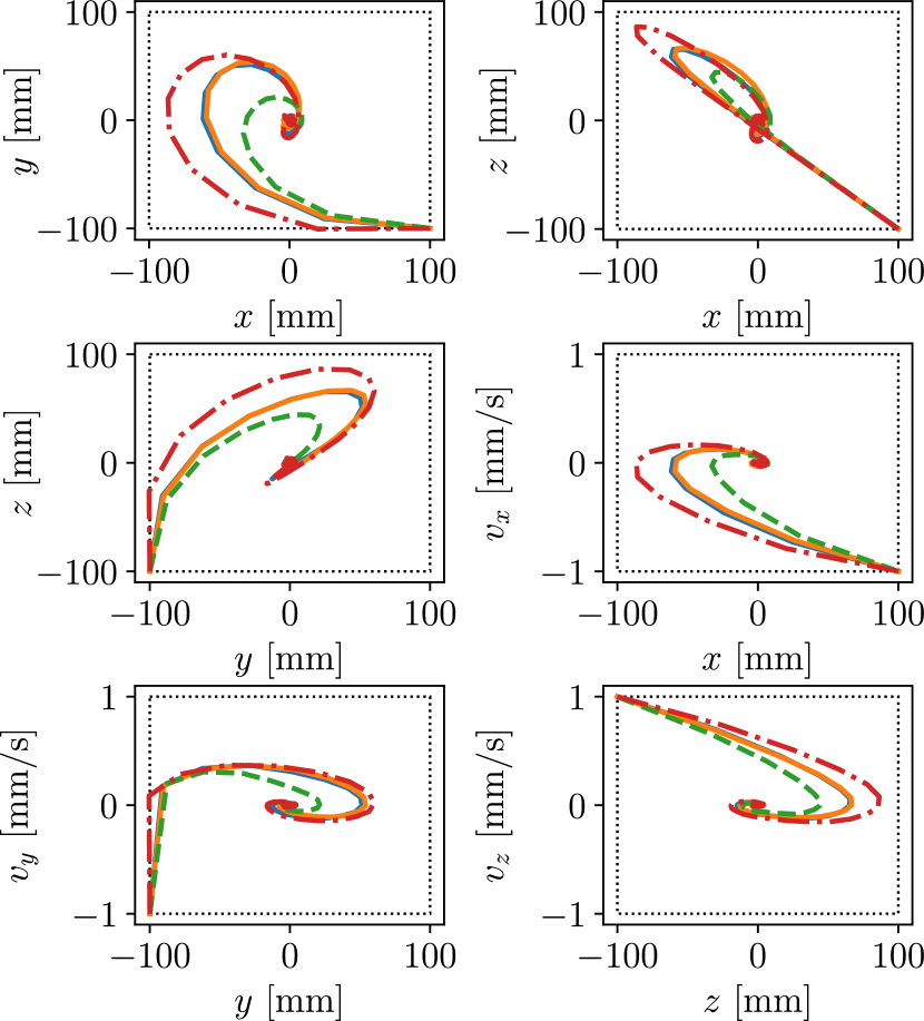
Figure 3: Projections of the transient response shown in dash dotted red for nominal MPC, dashed green for conservative RMPC, solid blue for our open-loop RMPC and solid orange for our semi-feedback RMPC. The dotted black rectangle shows the boundary of $\mathcal{I}$.

In each case the satellite is acted upon by all three of the uncertainty sources described above. It turns out that for this problem, Corollary 1 succeeds and so $\mathcal{I}=\mathcal{X}$. To demonstrate the conservatism exhibited by the conservative RMPC law, consider Figure 3 which shows the four controllers’ transient response when starting from a vertex of $\mathcal{I}$. While nominal MPC briefly exits $\mathcal{I}$, conservative RMPC tends to drive the satellite more quickly into the interior of $\mathcal{I}$ because it assumes more uncertainty than necessary. Open-loop and semi-feedback RMPC yield similar responses that are somewhere in between nominal and conservative MPC, staying within $\mathcal{I}$ and not avoiding the boundaries of $\mathcal{I}$ unnecessarily.

The RMPC law (13) enables the control engineer to work with a richer set of feasible parameters. For example, the required position accuracy can be increased to 5 cm without changing any other parameter, while doing so with the conservative RMPC law requires using $N\leq 2$. The open-loop RMPC law works for $N\leq 4$ before the passively propagated uncertainty “outgrows” $\mathcal{X}$. The less conservative semi-feedback RMPC law works for $N\leq 6$.

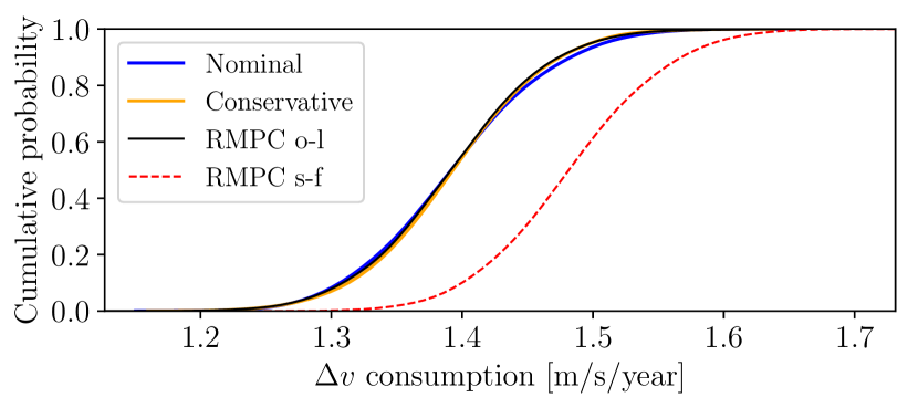
Figure 4: Fuel usage distribution for each controller from 2000 Monte Carlo simulations. RMPC o-l and s-f stand for our open-loop and semi-feedback RMPC laws respectively.

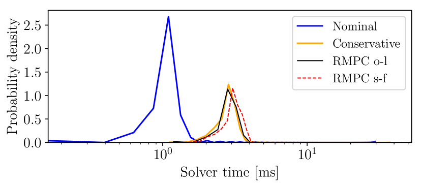
Figure 5: Optimization solver time distribution for each controller from 2000 Monte Carlo simulations. RMPC o-l and s-f stand for our open-loop and semi-feedback RMPC laws respectively.

Next, we compare the fuel consumption and computational efficiency of the three controllers. Fuel consumption is quantified by the sum of velocity increment magnitudes commanded per year as obtained from a linear regression, yielding units of m/s/year. This is common in space applications, where a mission is characterized by a “$\Delta v$ budget”. Computational efficiency is measured by the time taken to solve (13). Since both quantities are affected by the uncertainty realization, we run 2000 Monte Carlo simulations for each controller where the satellite is initialized at the origin and is controlled for a duration of four orbits.

Figure 4 shows a fuel consumption cumulative distribution plot using a Gaussian smoothing kernel. There is no statistically significant difference between the nominal MPC, conservative RMPC and open-loop RMPC laws. As expected, the embedded LQR controller increases the fuel consumption of semi-feedback RMPC by an average amount of $0.09$ m/s/year.

Figure 5 shows the solver time distribution for Python 2.7.15 with ECOS 2.0.7.post1 [26] in Ubuntu 18.04.1 with a 3.60 GHz Intel i7-6850K CPU and 64 GB of RAM. All four controllers have comparable solver times. The distributions reflect the problem difficulty hierarchy, wherein our RMPC laws are the most difficult due to second order cone constraints. On average, nominal MPC takes 1.1 ms, conservative and open-loop RMPC take 2.9 ms, and semi-feedback RMPC takes 3 ms. These differences are all statistically significant at the 99.9% confidence level. Generally speaking, SOCP problems are amenable to real-time implementation and we expect this to be the case here [23, 24, 25, 26].

VII Conclusion

This paper introduced a state and input dependent uncertainty model and a corresponding computationally efficient robust receding horizon control law based on second order cone programming. We have shown that the control law is recursively feasible and that both open-loop and semi-feedback implementations are possible. Simulations of a satellite system demonstrate that the approach is more versatile than RPMC based on an independent uncertainty model. The approach, however, is somewhat hampered by the ability to compute a robust controlled invariant set for the system. Recent work on controllable set computation for convex optimal control problems has the potential to remove this shortcoming [38].

VIII Acknowledgment

This research has been partly supported by the National Science Foundation, grant number CMMI-1613235, and was partially carried out at the Jet Propulsion Laboratory, California Institute of Technology, under a contract with the National Aeronautics and Space Administration. Government sponsorship acknowledged. The authors would like to extend special gratitude to Daniel P. Scharf, David S. Bayard, Jack Aldrich and Carl Seubert for their helpful insight and discussions.

References

- [1] C. R. Gates, “A simplified model of midcourse maneuver execution errors,” Tech. Rep. 32-504, JPL, Pasadena, CA, oct 1963.
- [2] S. V. Wagner, “Maneuver performance assessment of the Cassini spacecraft through execution-error modeling and analysis,” in AAS/AIAA Space Flight Mechanics Meeting, jan 2014.
- [3] H. Navvabi and A. H. D. Markazi, “New AFSMC method for nonlinear system with state-dependent uncertainty: Application to hexapod robot position control,” Journal of Intelligent & Robotic Systems, may 2018.
- [4] A. Bemporad and M. Morari, “Robust model predictive control: A survey,” in Robustness in identification and control, pp. 207–226, Springer London, 2007.
- [5] D. Q. Mayne, “Model predictive control: Recent developments and future promise,” Automatica, vol. 50, pp. 2967–2986, dec 2014.
- [6] J. Lee and Z. Yu, “Worst-case formulations of model predictive control for systems with bounded parameters,” Automatica, vol. 33, pp. 763–781, may 1997.
- [7] A. Bemporad, “Reducing conservativeness in predictive control of constrained systems with disturbances,” in Proceedings of the 37th IEEE Conference on Decision and Control (Cat. No.98CH36171), IEEE, 1998.
- [8] P. Scokaert and D. Q. Mayne, “Min-max feedback model predictive control for constrained linear systems,” IEEE Transactions on Automatic Control, vol. 43, no. 8, pp. 1136–1142, 1998.
- [9] E. C. Kerrigan and J. M. Maciejowski, “Feedback min-max model predictive control using a single linear program: robust stability and the explicit solution,” International Journal of Robust and Nonlinear Control, vol. 14, no. 4, pp. 395–413, 2004.
- [10] J. Löfberg, Minimax approaches to robust model predictive control. Dissertation (Ph.D.), Linköping University, 2003.
- [11] F. Blanchini, “Feedback control for linear time-invariant systems with state and control bounds in the presence of disturbances,” IEEE Transactions on Automatic Control, vol. 35, no. 11, pp. 1231–1234, 1990.
- [12] F. Blanchini, “Control synthesis for discrete time systems with control and state bounds in the presence of disturbances,” Journal of Optimization Theory and Applications, vol. 65, pp. 29–40, apr 1990.
- [13] F. Blanchini, “Constrained control for perturbed linear systems,” in 29th IEEE Conference on Decision and Control, IEEE, 1990.
- [14] F. Blanchini, “Ultimate boundedness control for uncertain discrete-time systems via set-induced Lyapunov functions,” IEEE Transactions on Automatic Control, vol. 39, no. 2, pp. 428–433, 1994.
- [15] D. Marruedo, T. Alamo, and E. Camacho, “Input-to-state stable MPC for constrained discrete-time nonlinear systems with bounded additive uncertainties,” in Proceedings of the 41st IEEE Conference on Decision and Control, 2002., IEEE, dec 2002.
- [16] G. Pin, D. Raimondo, L. Magni, and T. Parisini, “Robust model predictive control of nonlinear systems with bounded and state-dependent uncertainties,” IEEE Transactions on Automatic Control, vol. 54, pp. 1681–1687, jul 2009.
- [17] Y. Lee, B. Kouvaritakis, and M. Cannon, “Constrained receding horizon predictive control for nonlinear systems,” Automatica, vol. 38, pp. 2093–2102, dec 2002.
- [18] D. Limon, T. Alamo, and E. Camacho, “Robust stability of min-max MPC controllers for nonlinear systems with bounded uncertainties,” in Proceedings of the 16th Mathematical Theory of Networks and Systems Conference., 2004.
- [19] B. Açıkmeşe, J. M. Carson III, and D. S. Bayard, “A robust model predictive control algorithm for incrementally conic uncertain/nonlinear systems,” International Journal of Robust and Nonlinear Control, vol. 21, pp. 563–590, jul 2010.
- [20] S. V. Raković, “Set theoretic methods in model predictive control,” in Nonlinear Model Predictive Control, pp. 41–54, Springer Berlin Heidelberg, 2009.
- [21] M. Cannon and B. Kouvaritakis, “Optimizing prediction dynamics for robust MPC,” IEEE Transactions on Automatic Control, vol. 50, pp. 1892–1897, nov 2005.
- [22] T. D. Goodson, “Execution-error modeling and analysis of the GRAIL spacecraft pair,” in AAS/AIAA Space Flight Mechanics Meeting, aug 2013.
- [23] D. Dueri, J. Zhang, and B. Açıkmeşe, “Automated custom code generation for embedded, real-time second order cone programming,” IFAC Proceedings Volumes, vol. 47, no. 3, pp. 1605–1612, 2014.
- [24] D. Dueri, B. Açıkmeşe, D. P. Scharf, and M. W. Harris, “Customized real-time interior-point methods for onboard powered-descent guidance,” Journal of Guidance, Control, and Dynamics, vol. 40, pp. 197–212, feb 2017.
- [25] M. N. Zeilinger, D. M. Raimondo, A. Domahidi, M. Morari, and C. N. Jones, “On real-time robust model predictive control,” Automatica, vol. 50, pp. 683–694, mar 2014.
- [26] A. Domahidi, E. Chu, and S. Boyd, “ECOS: An SOCP solver for embedded systems,” in 2013 European Control Conference (ECC), IEEE, jul 2013.
- [27] S. Boyd and L. Vandenberghe, Convex Optimization. Cambridge University Press, 2004.
- [28] F. Blanchini and S. Miani, Set-Theoretic Methods in Control. Springer International Publishing, 2015.
- [29] M. Kvasnica, B. Takács, J. Holaza, and D. Ingole, “Reachability analysis and control synthesis for uncertain linear systems in MPT,” IFAC-PapersOnLine, vol. 48, no. 14, pp. 302–307, 2015.
- [30] S. V. Raković, E. C. Kerrigan, D. Q. Mayne, and J. Lygeros, “Reachability analysis of discrete-time systems with disturbances,” IEEE Transactions on Automatic Control, vol. 51, pp. 546–561, apr 2006.
- [31] M. Baotić, “Polytopic computations in constrained optimal control,” Automatika, Journal for Control, Measurement, Electronics, Computing and Communications, vol. 50, pp. 119–134, 2009.
- [32] I. Kolmanovsky and E. G. Gilbert, “Theory and computation of disturbance invariant sets for discrete-time linear systems,” Mathematical Problems in Engineering, vol. 4, no. 4, pp. 317–367, 1998.
- [33] P. J. Antsaklis and A. N. Michel, A Linear Systems Primer. Birkhäuser Boston, 2007.
- [34] B. Açıkmeşeand S. R. Ploen, “Convex programming approach to powered descent guidance for mars landing,” Journal of Guidance, Control, and Dynamics, vol. 30, pp. 1353–1366, sep 2007.
- [35] B. Açıkmeşeand L. Blackmore, “Lossless convexification of a class of optimal control problems with non-convex control constraints,” Automatica, vol. 47, pp. 341–347, feb 2011.
- [36] L. Blackmore, B. Açıkmeşe, and J. M. Carson III, “Lossless convexification of control constraints for a class of nonlinear optimal control problems,” Systems & Control Letters, vol. 61, pp. 863–870, aug 2012.
- [37] T. Schouwenaars, Safe trajectory planning of autonomous vehicles. Dissertation (Ph.D.), Massachusetts Institute of Technology, 2006.
- [38] D. Dueri, S. V. Raković, and B. Açıkmeşe, “Consistently improving approximations for constrained controllability and reachability,” in 2016 European Control Conference (ECC), IEEE, jun 2016.