Dynamical properties of acoustic-gravity waves in the atmosphere

Abstract

We study the dynamical behaviors of a system of five coupled nonlinear equations that describes the dynamics of acoustic-gravity waves in the atmosphere. A linear stability analysis together with the analysis of Lyapunov exponents spectra are performed to show that the system can develop from ordered structures to chaotic states. Numerical simulation of the system of equations reveals that an interplay between the order and chaos indeed exists depending on whether the control parameter $s_{1}$, associated with the density scale height of acoustic-gravity waves, is below or above its critical value.

1 Introduction

The nonlinear dynamics of low-frequency finite amplitude acoustic-gravity waves has been studied by a number of authors because of their relevance in atmospheric disturbances [1, 2, 3, 4, 5, 6, 7]. The latter appear due to various meteorological conditions including different pressure and density gradients, as well as the presence of shear flows [5]. It has been shown that the nonlinear acoustic-gravity waves can appear in the forms of localized solitary vortices [1, 5], ordered structures [8], as well as chaos [9] and turbulence [10].

In a paper [4], Stenflo deduced a system of five coupled equations that describes the essential features of low-frequency atmospheric disturbances. His starting point was the most commonly used model equations for two-dimensional acoustic-gravity waves of the form [3]

$$D_{t}\left(\nabla^{2}\psi-\frac{1}{4H^{2}}\psi\right)=-\partial_{x}\chi,$$ (1)

$$D_{t}\chi=\omega^{2}_{g}\partial_{x}\psi,$$ (2)

where $\nabla^{2}\equiv{\partial^{2}}/{\partial x^{2}}+{\partial^{2}}/{\partial z^{2}}$, $D_{t}\equiv\partial_{t}+{\bf v}\cdot\nabla$, $H$ is the density scale height, $\omega_{g}$ is the Brunt-Väisälä frequency, $\psi(x,z)$ is the velocity potential in which $z$ represents the vertical direction, and $\chi(x,z)$ is the normalized density perturbation.

Substitution of the expression for the velocity, i.e., ${\bf v}=-\partial_{z}\psi\hat{x}+\partial_{x}\psi\hat{z}$ into Eqs. (1) and (2) results in

$$\begin{split}\frac{\partial}{\partial t}\nabla^{2}\psi-\frac{1}{4H^{2}}\frac{\partial\psi}{\partial t}&=-J(\psi,\nabla^{2}\psi)-\frac{\partial\chi}{\partial x},\\ \frac{\partial\chi}{\partial t}&=-J(\psi,\chi)+\omega_{g}^{2}\frac{\partial\psi}{\partial x},\end{split}$$ (3)

where $J(f,g)=\left({\partial f}/{\partial x}\right)\left({\partial g}/{\partial z}\right)-\left({\partial g}/{\partial x}\right)\left({\partial f}/{\partial z}\right)$ is the Jacobian.
For a class of solutions of Eqs. (3) of the form

$$\begin{split}\psi&=\left[a(t)\sin(k_{0}x)+b(t)\cos(k_{0}x)+\omega_{0}\right]z/k_{0},\\ \chi&=\left[\alpha(t)\sin(k_{0}x)+\beta(t)\cos(k_{0}x)+\gamma(t)\right]z,\end{split}$$ (4)

where $k_{0}$ and $\omega_{0}$ are constants, Stenflo [4] derived the following set of coupled equations for acoustic-gravity waves, given by,

$$\begin{split}\partial_{t}a+\tilde{\omega_{0}}b+s_{1}\beta&=-\nu_{1}a,\\ \partial_{t}b-\tilde{\omega_{0}}a-s_{1}\alpha&=-\nu_{1}b,\\ \partial_{t}\alpha+\omega_{0}\beta-s_{2}b\gamma+\omega^{2}_{g}b&=-\nu_{2}\alpha,\\ \partial_{t}\beta-\omega_{0}\alpha+s_{2}a\gamma-\omega^{2}_{g}a&=-\nu_{2}\beta,\\ \partial_{t}\gamma+a\beta-\alpha b&=-\nu_{3}\gamma.\end{split}$$ (5)

Here, the terms containing $\nu_{1}$ and $\nu_{2}$ appear when one considers, in addition with the other effects, the dissipative terms proportional to $\nabla^{4}\psi$ and $\nabla^{2}\psi$ respectively in Eqs. (1) and (2), and the term proportional to $\nu_{3}$ corresponds to the damping term. Also, as in Ref. [4], $\omega_{0}$ and $\omega_{g}$ are two control parameters with $\tilde{\omega}_{0}={\omega_{0}}/\left(1+1/4Hk_{0}^{2}\right)=s_{1}\omega_{0}$, $s_{1}=\left(1+1/4H^{2}k_{0}^{2}\right)^{-1}$ and $s_{2}=1$.

In this paper, we numerically study the dynamical behaviors of Eq. (5) in absence of the dissipative and damping effects. By means of the linear stability analysis and the Lyapunov exponent spectra, it is seen that the nonlinear interaction of acoustic-gravity waves can result into an ordered structure or chaos depending on whether the parameter $s_{1}$, associated with the density scale height $H$, is below or above its critical value.

2 Dynamical Properties

In this section, we numerically study the dynamical properties of Eqs. (5). We focus mainly on the development of chaos as well as the tendency to form ordered structures in absence of the dissipative effects (i.e., terms proportional to $\nu_{1}$, $\nu_{2}$ and $\nu_{3}$). Thus, setting $\nu_{1}=\nu_{2}=\nu_{3}=0$ and for convenience, redefining the variables, namely, $a=u,~{}b=v,~{}\alpha=x,~{}\beta=y$ and $\gamma=z$, Eq. (5) can be recast as

$$\begin{split}\frac{du}{dt}&=-\tilde{\omega}_{0}v-{s_{1}}y,\\ \frac{dv}{dt}&=\tilde{\omega}_{0}u+{s_{1}}x,\\ \frac{dx}{dt}&=-\omega_{0}y+vz-{\omega_{g}}^{2}v,\\ \frac{dy}{dt}&=\omega_{0}x-uz+{\omega_{g}}^{2}u,\\ \frac{dz}{dt}&=-uy+xv.\end{split}$$ (6)

2.1 Linear stability analysis

In order to perform the stability analysis of the system (6), we first find its fixed points $\left(u_{0},v_{0},x_{0},y_{0},z_{0}\right)$. These can be obtained by equating the right-hand sides of Eq. (6) to zero and finding solutions for $u,~{}v,~{}x,~{}y$ and $z$. Thus, the fixed points so obtained are the origin $O=(0,0,0,0,0)$ and $P=\left(0,0,0,0,\omega_{0}^{2}+\omega_{g}^{2}\right)$. Next, around the fixed points, we apply the perturbations of the forms: $u^{\prime}=u-u_{0},~{}v^{\prime}=v-v_{0},~{}x^{\prime}=x-x_{0},~{}y^{\prime}=y-y_{0}$ and $z^{\prime}=z-z_{0}$ to obtain a linearized system of perturbation equations: $d{\bf X}/dt=J{\bf X}$, where ${\bf X}=(u^{\prime},v^{\prime},x^{\prime},y^{\prime},z^{\prime})$ and $J$ is the Jacobian matrix. For each fixed point, the eigenvalues $\lambda$ can be obtained from the corresponding eigenvalue problem $J{\bf X}=\lambda{\bf X}$. The stability of the system (6) about the fixed points can then be studied by the nature of these eigenvalues.

The Jacobian matrix corresponding to the fixed point $O$ is given by

$$J_{O}=\begin{bmatrix}0&-\tilde{\omega}_{0}&0&-{s_{1}}&0\\ \tilde{\omega}_{0}&0&{s_{1}}&0&0\\ 0&-\omega_{g}^{2}&0&-\omega_{0}&0\\ \omega_{g}^{2}&0&\omega_{0}&0&0\\ 0&0&0&0&0\end{bmatrix}$$ (7)

and the corresponding eigenvalues of the matrix $J_{O}$ are given by $\lambda=0$ and

$$\lambda=\pm\frac{1}{\sqrt{2}}\left(-B\pm\sqrt{B^{2}-4C}\right)^{1/2},$$ (8)

where $B=\omega_{0}^{2}+\tilde{\omega}_{0}^{2}+2s_{1}\omega_{g}^{2}$ and $C=\left(s_{1}\omega_{g}^{2}-\omega_{0}\tilde{\omega}_{0}\right)^{2}$. We note that since $C>0$ and $B>0$ for $0<s_{1}<1$, the values of $\lambda$ in Eq. (8) are purely imaginary, i.e., $\Re\lambda=0$, implying that the fixed point $O$ corresponds to a stable center.

Next, for the stability of the system (6) around the fixed point $P$, we apply the similar perturbations as discussed before, i.e., $u^{\prime}=u,~{}v^{\prime}=v,~{}x^{\prime}=x,~{}y^{\prime}=y$ but with $z^{\prime}=z-\left(\omega_{0}^{2}+\omega_{g}^{2}\right)$. The corresponding Jacobian matrix $J_{P}$ and the corresponding eigenvalues $\lambda$ are, respectively, given by

$$J_{P}=\begin{bmatrix}0&-\tilde{\omega}_{0}&0&-{s_{1}}&0\\ \tilde{\omega}_{0}&0&{s_{1}}&0&0\\ 0&{\omega_{0}}^{2}&0&-\omega_{0}&0\\ -{\omega_{0}}^{2}&0&\omega_{0}&0&0\\ 0&0&0&0&0\end{bmatrix},$$ (9)

$\lambda=0$ and

$$\lambda=\pm\frac{\omega_{0}}{\sqrt{2}}\left[-(1-s_{1})^{2}\pm(1+s_{1})\sqrt{\left(1-s_{1}\right)^{2}-4s_{1}}\right]^{1/2},$$ (10)

in which we have used the expression $\tilde{\omega}_{0}=s_{1}\omega_{0}$. From Eq. (10), we note that the values of $\lambda$ become purely imaginary for $0<s_{1}\lesssim 0.17$, and in this case, the the fixed point $P$ corresponds to a stable center. However, for values of $s_{1}$ in $0.17<s_{1}<1$, $\lambda$ has complex conjugate values with positive and negative real parts. Thus, it turns out that the system may be unstable (with at least one $\Re\lambda>0$) around the fixed point $P$ for $0.17<s_{1}<1$. From the above analysis it follows that the parameter $s_{1}$, which typically depends on the density scale height $H$ for acoustic-gravity waves, plays a crucial role for the stability and instability of the system (6) about the fixed points $O$ and $P$. In fact, as the the density scale height $H$ increases and so is $s_{1}$, the system’s stability tends to break down, which can lead to the development of chaos as will be shown later.

Figure 1 shows the bifurcation diagram for stable and unstable regions corresponding to the fixed points $O$ and $P$. We plot $\lambda$, given by Eqs. (8) and (10), with respect to the parameter $s_{1}$ $(0<s_{1}<1)$. The dash-dotted line represents $\lambda=0$ corresponding to the fixed point $O$. Also, for the fixed point $P$, $\Re\lambda=0$ in the interval $0<s_{1}\lesssim 0.17$. So, the system is stable around both the fixed points in the domain $0<s_{1}\lesssim 0.17$. However, beyond this domain, i.e., in $0.17<s_{1}<1$, the system is shown to be unstable around the fixed point $P$. In Fig. 1, the upper (solid line) and lower (dashed line) branches are the plots of $\lambda$ corresponding to the $\pm$ sign in the square brackets in Eq. (10).

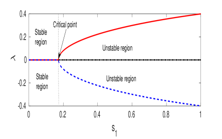
Figure 1: Pitchfork bifurcation diagram showing the stable and unstable regions of the system (6) around the fixed points $O$ and $P$. While the system is stable in the region $0<s_{1}\lesssim 0.17$ where $\lambda=0$ or $\Re\lambda=0$, it exhibits instability in the domain $0.17\lesssim s_{1}<1$ with $\Re\lambda>0$. The upper (solid red line) and lower (dashed blue line) branches are corresponding to the $\pm$ sign in the square brackets of the expression for $\lambda$ [Eq. (10)]. The other parameter values are $\omega_{0}=0.4$, $\omega_{g}=1.01$, and $\tilde{\omega}_{0}=s_{1}\omega_{0}$.

In the next subsection 2.2, we will calculate the Lyapunov exponents spectra to verify the existence of chaos with variations of the parameters $s_{1}$, $\omega_{0}$ and $\omega_{g}$.

2.2 Lyapunov exponents

In order to calculate the Lyapunov exponents, we solve the system of equations (6) with the initial condition $X(0)=\left(u(0),v(0),x(0),y(0),z(0)\right)$. If the system (6) is recast as $\dot{X}=\left(\dot{u}(t),\dot{v}(t),\dot{x}(t),\dot{y}(t),\dot{z}(t)\right)$, its variational form of equation is given by

$$\frac{d}{dt}DX(t)=J_{L}(t)DX(t),$$ (11)

where $D\equiv d/dt$, $DX(0)=I_{5}$ with $I_{5}$ denoting the identity matrix of order $5$ and $J_{L}(t)$ the Jacobian matrix evaluated at the initial value $X(0)$, given by,

$$J_{L}(t)=\begin{bmatrix}0&-\tilde{\omega}_{0}&0&-{s}_{1}&0\\ \tilde{\omega}_{0}&0&{s}_{1}&0&0\\ 0&z(t)-\omega_{g}^{2}&0&-\omega_{0}&v(t)\\ \omega_{0}^{2}-z(t)&0&\omega_{0}&0&u(t)\\ -y(t)&x(t)&v(t)&-u(t)&0\end{bmatrix}.$$ (12)

Since $DX(0)$ is non-singular and so is $DX(t)$, the solution of Eq. (11) is given by

$$\Lambda=\lim_{t\to\infty}\frac{1}{2t}\ln\left[\left(D{X(t)})^{T}D{X(t)}\right)\right],$$ (13)

from which the Lyapunov exponents are obtained as the eigenvalues $\lambda_{i},~{}i=1,...,5$ of the matrix $\Lambda$. Given a fixed initial condition $X(0)$ of the dynamical system, the change of particle’s orbit can be found by the Liouville’s formula: $\Delta(t)=\text{tr}(J_{L}(t))\Delta_{t}$, where $\Delta_{t}\equiv\det DX(t)$, $\Delta_{0}\equiv\det DX(0)=\det I_{5}=1>0$ and ‘tr’ denotes the trace of the matrix $J_{L}(t)$. Thus, for the system (6) we have $\det{DX(t)}=\exp(\int_{0}^{t}\text{tr}(J_{L}(t))dt=1>0$, implying that at least one eigenvalue $\lambda_{i}$ is positive, and so a chaotic orbit exists for a certain time period $[0~{}t]$.

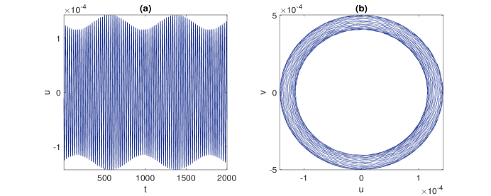
Figure 2: Stable oscillations: (a) the time series and (b) the phase-space diagram showing that the equilibrium point $O$ corresponds to the stable center. The parameter values are $\omega_{0}=0.01$, $s_{1}=0.61$, $\omega_{g}=1.01$ and $\tilde{\omega}_{0}=s_{1}.\omega_{0}=0$.

3 Numerical analysis

We study the dynamical behaviors of solutions of the system (6). To this end, we numerically integrate Eq. (6) by using the 4-th order Runge-Kutta scheme with a time step $\Delta t=10^{-3}$. The results are displayed in Figs. 2 to 4. We note that for certain ranges of values of the parameters $\omega_{0}$, $\omega_{g}$ and $s_{1}$, the system can exhibit stable solutions together with the quasi-periodic and chaotic states. We study these behaviors in three different cases as follows.

Stable Center: We note that for $\omega_{0}=0$, and any values of $\omega_{g}$ and $s_{1}$ in $0<s_{1}<1$, the eigenvalues corresponding to the fixed point $O$ are zero and purely imaginary, while those about the fixed point $P$ are all zero. In this case, the system exhibits stable solutions about the fixed points $O$ and $P$. The system also possesses a class of stable solutions for $\omega_{0}>0$, $\omega_{g}>0$ and $0<s_{1}\lesssim 0.17$ (cf. Sec. 2.1 and the bifurcation diagram in Fig. 1). The corresponding time series (a) and the phase space plots (b) are shown in Fig. 2.

Quasi-periodicity: From the linear stability analysis and the bifurcation diagram (See Fig. 1) it is evident that the system tends to loose its stability for $s_{1}>0.17$ and any positive values of the frequencies $\omega_{0}$ and $\omega_{g}$. In fact, there are two subregions of the parameter $s_{1}$: $0.17<s_{1}\lesssim s_{2}$ and $s_{2}\lesssim s_{1}<1$. In the former, the system exhibits quasi-periodicity while in the latter it has chaotic behaviors. However, it is very difficult to find a particular region of $s_{1}$ in which the quasi-periodicity transits into the chaotic states. Usually, in the quasi-periodic region, we observe a stable torus whereas in the chaotic region, the torus structure breaks down, giving rise to a chaotic structure. For a suitable choice of the initial condition $(-\omega_{0}k_{1},-\omega_{0}k,k,k_{1},-\omega_{0}^{2}-\omega_{g}^{2})$, where $k=0.9$ and $k_{1}=0.8$ together with the parameters $\omega_{0}=1.5$, $\omega_{g}=1.01$ and $s_{1}=0.31$ with $\tilde{\omega}_{0}=s_{1}\omega_{0}=0.465$, Fig. 3 shows that the torus structure forms at $s_{1}=0.31$.

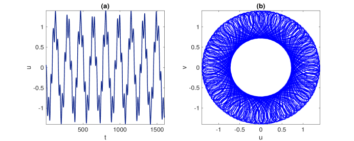
Figure 3: Subplots (a) and (b) are, respectively, the time series and the phase space (torus) showing the quasi-periodicity of the system (6) with parameter values $\omega_{0}=1.5$, $s_{1}=0.31$, $\omega_{g}=1.01$ and $\tilde{\omega}_{0}=s_{1}\omega_{0}=0.465$.

Chaotic property: We note that of the two fixed points $O$ and $P$, the point $O$ always gives a stable center in every possible regions of the parameters and the initial conditions. However, for the other fixed point $P$, we have a stable center in the region of $0<s_{1}\lesssim 0.17$, while in the other region $0.17<s_{1}<1$, the system exhibits either quasi-periodicity or chaos. For a suitable choice of the initial condition and the parameters, namely, $(-\omega_{0}k_{1},-\omega_{0}k,k,k_{1},-\omega_{0}^{2}-\omega_{g}^{2})$ with $k=5$, $k_{1}=5.8$, $\omega_{0}=1.5$, $\omega_{g}=1.01$, $s_{1}=0.91$, and $\tilde{\omega}_{0}=s_{1}\omega_{0}=1.365$, we show that the system (6), indeed, exhibits chaos, i.e., the torus which forms at $s_{1}=0.31$ (see Fig. 3) breaks down at a higher value of $s_{1}=0.91$ (Fig. 4). The corresponding time series [subplot(a)], the phase space [subplot(b)] and the Lyapunov exponents [subplot(c)] are shown in Fig. 4. Here, the appearance of at least one positive Lyapunov exponent ensures the existence of chaos.

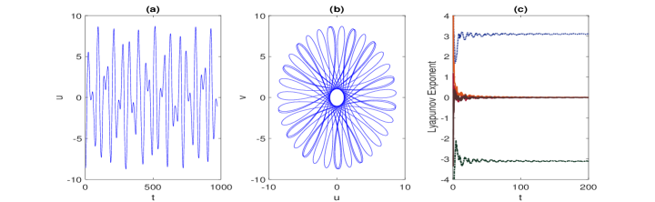
Figure 4: The chaotic time series (a), the chaotic phase space (b) and the Lyapunov exponents (c) are shown with parameters $\omega_{0}=1.5$, $s_{1}=0.91$, $\omega_{g}=1.01$, and $\tilde{\omega}_{0}=s_{1}\omega_{0}=1.365$.

4 Conclusion

We have investigated the dynamical properties of five nonlinear coupled Stenflo equations [4] that describe the evolution of acoustic-gravity waves in atmospheric disturbances. A linear stability analysis together with the analysis of Lyapunov exponents spectra are carried out for different values of the control parameters. It is found that the parameter $s_{1}$, which typically depends on the density scale height of acoustic-gravity waves, plays a vital role for the existence of ordered structures as well as chaos of the Stenflo equations. While the system exhibits stable solutions in the region $0<s_{1}\lesssim 0.17$, it can describe chaotic behaviors in the other region $0.17<s_{1}<1$. The present results should be useful for understanding the chaotic properties of the atmospheres of the Earth and other planets.

References

- [1] Stenflo, L. 1987. Acoustic solitary vortices. Physics of Fluids 30, 3297.
- [2] Stenflo, L. 1991. Equations describing solitary atmospheric waves. Physica Scripta 43, 599.
- [3] Stenflo, L., Stepanyants, Yu.A. 1995. Acoustic-gravity modons in the atmosphere. Annales Geophysicae 13, 973.
- [4] Stenflo, L. 1996. Nonlinear equations for acoustic gravity waves. Physics Letters A 222, 378.
- [5] Jovanovic, D., Stenflo, L. Shukla, P.K. 2002. Acoustic-gravity nonlinear structures. Nonlinear Processes in Geophysics 9, 333.
- [6] Mendonca, J.T., Stenflo, L. 2015. Acoustic-gravity waves in the atmosphere: from Zakharov equations to wave-kinetics. Physica Scripta 90, 055001.
- [7] Kaladze, T.D., Pokhotelov, O.A., Shah, H.A., Khan, M.I., Stenflo, L. 2008. Acoustic-gravity waves in the Earth’s ionosphere. Journal of Atmospheric and Solar-Terrestrial Physics 70, 1607.
- [8] Park, J., Han, B-S, Lee, H., Jeon, Y-L, Baik, J-J 2016. Stability and periodicity of high-order Lorenz–Stenflo equations. Physica Scripta 91, 065202.
- [9] Banerjee, S., Saha, P., Roy Chowdhury, A. 2001. Chaotic Scenario in the Stenflo Equations. Physica Scripta 63, 177.
- [10] Shaikh, D., Shukla, P.K., Stenflo, L. 2008. Spectral properties of acoustic gravity wave turbulence. Journal of Geophysical Research 113, D06108.