A comparative evaluation of novelty detection algorithms for discrete sequences

Abstract

The identification of anomalies in temporal data is a core component of numerous research areas such as intrusion detection, fault prevention, genomics and fraud detection. This article provides an experimental comparison of the novelty detection problem applied to discrete sequences. The objective of this study is to identify which state-of-the-art methods are efficient and appropriate candidates for a given use case. These recommendations rely on extensive novelty detection experiments based on a variety of public datasets in addition to novel industrial datasets. We also perform thorough scalability and memory usage tests resulting in new supplementary insights of the methods’ performance, key selection criterion to solve problems relying on large volumes of data and to meet the expectations of applications subject to strict response time constraints.

1 Introduction

Novelty detection is an unsupervised learning problem and an active research area Aggarwal2015outlier ; Hodge2004outlier . Given a set of training samples, novelty detection is the task of classifying new test samples as nominal when the test data relates to the training set, or as anomalous when they significantly differ. Anomalous data is called novelties or anomalies and is assumed to be generated by a different generative process. Since novelty detection can be considered a one-class classification problem, it has also been described as a semi-supervised problemChandola2012survey when the training set is exempt of outliers. While most anomaly detection problems deal with numerical dataemmott2016anomaly ; breunig2000lof ; Ramaswamy2000kNN , novelty detection methods have been successfully applied to categorical dataHodge2004outlier , time-seriesMarchi2015denoising ; Zbigniew2004change ; Taylor2018prophet , discrete sequenceschandola2008comparative ; stide1999intrusions ; Cohen1995115 and mixed data typesDomingues2018DGP .

This paper surveys the problem of detecting anomalies in temporal data, specifically in discrete sequences of events which have a temporal order. Such a problem can be divided into two categories. The first one is change point detection, where datasets are long sequences in which we seek anomalous and contiguous subsequences, denoting a sudden change of behavior in the data. Use cases relating to this problem are sensor readingsZbigniew2004change and first story detectionPetrovic2010story . A second category considers datasets as sets of sequences, and targets the detection of anomalous sequences with respect to nominal samples. Our study focuses on the latter, which encompasses use cases such as protein identification for genomicschandola2008comparative ; sun2006pst , fraud and intrusion detectionmaxion2002masquerade ; stide1999intrusions ; chandola2008comparative and user behavior analysis (uba)sculley2006compression .

While this is a matter of interest in the literature, most reviews addressing the issue focus on theoretical aspectsGupta2014survey ; Chandola2012survey , and as such do not assess and compare performance. Chandola et al.chandola2008comparative showcase an experimental comparison of novelty detection methods for sequential data, although this work uses a custom metric to measure the novelty detection capabilities of the algorithms and misses methods which have been recently published in the field. Our work extends previous studies by bringing together the following contributions: (i) comparison of the novelty detection performance for 12 algorithms, including recent developments in neural networks, on 81 datasets containing discrete sequences from a variety of research fields; (ii) assessment of the robustness for the selected methods using datasets contaminated by outliers, with contrast to previous studies which rely on clean training data; (iii) scalability measurements for each algorithm, reporting the training and prediction time, memory usage and novelty detection capabilities on synthetic datasets of increasing samples, sequence length and anomalies; (iv) discussion on the interpretability of the different approaches, in order to provide insights and motivate the predictions resulting from the trained model. To our knowledge, this study is the first to perform an evaluation of novelty detection methods for discrete sequences with so many datasets and algorithms. This work is also the first to assess the scalability of the selected methods, which is an important selection criterion for processes subject to fast response time commitments, in addition to resource-constrained systems such as embedded systems.

The paper is organized as follows: Section 2 presents the state-of-the-art of novelty detection methods, Section 3 details the real-world and synthetic datasets used for the study, in addition to the relevant metrics and parameters, Sections 4 and 5 report the results and conclusions of the work.

2 Methods

The current section details novelty detection methods from the literature. In order to provide recommendations relevant to real-world use cases, only methods satisfying the following constraints were selected: (1) the method accepts discrete sequences of events as input, where events are represented as categorical samples; (2) the sequences fed to the method may have variable lengths, which implies a dedicated support or a tolerance for padding; (3) the novelty detection problem induces a distinct training and testing dataset. As such, the selected approach should be able to perform predictions on unseen data which was not presented to the algorithm during the training phase; (4) subject to user inputs and system changes, the set of discrete symbols in the sequences (alphabet) of the training set cannot be assumed to be complete. The algorithm should support new symbols from the test set; (5) in order to perform an accurate evaluation of its novelty detection capabilities and to provide practical predictions on testing data, the method should provide continuous anomaly scores rather than a binary decision. This last point allows for a ranking of the anomalies, and hence a meaningful manual validation of the anomalies, or the application of a user-defined threshold in the case of automatic intervention. The ranking of anomalies is also required by the performance metric used in the study and described in section 3.1.

2.1 Hidden Markov Model

Hidden Markov Models (hmms)RabinerHMM18626 are popular graphical models used to describe temporal data and generate sequences. The approach fits a probability distribution over the space of possible sequences, and is widely used in speech recognition and protein modelling. An hmm is composed of $N$ states which are interconnected by state-transition probabilities, each state generating emissions according to its own emission probability distribution and the previous emission. To generate a sequence, an initial state is first selected based on initial probabilities. A sequence of states is then sampled according to the transition matrix of the hmm. Once the sequence of states is obtained, each state emits a symbol based on its emission distribution. The sequence of emissions is the observed data. Based on a dataset composed of emission sequences, we can achieve the inverse process, i.e. estimate the transition matrix and the emission distributions of a hmm from the emissions observed. Possible sequences of hidden states leading to these emissions are thus inferred during the process. Once we obtain a trained hmm $\lambda=(A,B,\pi)$ with $A$ the transition matrix, $B$ describing the emission probabilities and $\pi$ the initial state probabilities, we can compute the normalized likelihood of a sequence and use it as a score to detect novelties.

2.2 Distance-based methods

Distance-based approaches rely on pairwise distance matrices computed by applying a distance function to each pair of input sequences. The resulting matrix is then used by clustering or nearest-neighbor algorithms to build a model of the data. At test time, a second distance matrix is computed to perform scoring, which contains the distance between each test sample and the training data.

2.2.1 Distance metrics

lcs is the longest common subsequenceBergroth2000Survey shared between two sequences. A common subsequence is defined as a sequence of symbols appearing in the same order in both sequences, although they do not need to be consecutive. For example, ${\textsc{lcs}}(\textsc{xmjyauz},\textsc{mzjawxu})=\textsc{mjau}$. Since lcs expresses a similarity between sequences, we use the negative lcs to obtain a distance.

The Levenshtein distance1966levenshtein , also called the edit distance, is a widely used metric which computes the difference between two strings or sequences of symbols. It represents the minimum number of edit operations required to transform one sequence into another, such as insertions, deletions and substitutions of individual symbols.

Both metrics are normalized by the sum of the sequence lengths (equation 1), which makes them suitable for sequences of different length.

$$distance(x,y)=\frac{metric(x,y)}{|x|+|y|}$$ (1)

2.2.2 Algorithms

The k-nearest neighbors (k-nn) algorithm is often used for classification and regression. In the case of classification, k-nn assigns to each test sample the label the most represented among its k nearest neighbors from the training set. In Ramaswamy2000kNN , the scoring function used to detect outliers is the distance $d(x,n_{k})$ or $d_{k}(x)$ between a point $x$ and its $k^{th}$ nearest neighbor $n_{k}$. This approach was applied to sequences in chandola2008comparative using the lcs metric, and outperformed methods such as hmm and ripper.

Local outlier factor (lof) breunig2000lof also studies the neighborhood of test samples to identify anomalies. It compares the local density of a point $x$ to the local density of its neighbors by computing the reachability distance $rd_{k}(x,y)$ between $x$ and each of its k-nearest neighbors $n_{i}$.

$$rd_{k}(x,n_{i})=\max(d_{k}(n_{i}),d(x,n_{i}))$$ (2)

The computed distances are then aggregated into a final anomaly score detailed in breunig2000lof . The method showed promising results when applied to intrusion detection Lazarevic2003Study .

k-medoids park2009kmedoids is a clustering algorithm which uses data points from the training set, also called medoids, to represent the center of a cluster. The algorithm first randomly samples k medoids from the input data, then cluster the remaining data points by selecting the closest medoid. The medoids of each cluster are further replaced by a data point from the same cluster which minimizes the sum of distances between the new medoid and the points in the cluster. The method uses expectation-maximization and is very similar to k-means, although the latter uses the arithmetic mean of a cluster as a center, called centroid. Since k-means requires numerical data and is more sensitive to outliers park2009kmedoids , it was not selected for this study. We use the distance to the closest medoid to detect anomalies, which is the method used in Budalakoti2009airline and budalakoti2006anomaly . Both papers used the lcs metric to preprocess the data given to k-medoids.

2.3 Window-based techniques

The two following methods observe subsequences of fixed length, called windows, within a given sequence to identify abnormal patterns. This workflow requires to preprocess the data by applying a sliding window to each sequence, shifting the window by one symbol at each iteration and resulting in a larger dataset due to overlapping subsequences.

t-stidestide1999intrusions , which stands for threshold-based sequence time-delay embedding, uses a dictionary or a tree to store subsequences of length k observed in the training data, along with their frequency. Once this model is built, the anomaly score of a test sequence is the number of subsequences within the sequence which do not exist in the model, divided by the number of windows in the test sequence. For increased robustness, subsequences having a frequency lower than a given threshold are excluded from the model. This increases the anomaly score for uncommon patterns, and allows the algorithm to handle datasets contaminated by anomalous sequences. This scoring method is called Locality Frame Count (lfc) and was applied to intrusion detectionstide1999intrusions where it performed almost as well as hmm at a reduced computational cost.

ripper Cohen1995115 is a supervised classifier designed for association rule learning. The training data given to the algorithm is divided into a set of sequences of length k, and the corresponding labels. For novelty detection, subsequences are generated by a sliding window, and the label is the symbol following each subsequence. This allows ripper to learn rules predicting upcoming events. This method was applied to intrusion detection in lee1997learning . To build an anomaly score for a test sequence, the authors retrieve the predictions obtained for each subsequence, along with the confidence of the rule which triggered the prediction. Each time a prediction does not match the upcoming event, the anomaly score is increased by $confidence*100$. The final score is then divided by the number of subsequences for normalization.

2.4 Pattern mining

Sequential Pattern Mining (SPM) consists in the unsupervised discovery of interesting and relevant subsequences in sequential databases. A recent algorithm from this field is Interesting Sequence Miner (ism)Fowkes2016ISM , a probabilistic and generative method which learns a set of patterns leading to the best compression of the database. From a training set, ism learns a set of interesting subsequences ranked by probability and interestingness. To score a test sequence, we count the number of occurrences of each interesting pattern returned by ism, and multiply the number of occurrences by the corresponding probability and interestingness. This score is normalized by the length of the test sequence, a low score denoting an anomaly. While alternatives to ism exist in the literaturegan2018survey , few provide both a probabilistic framework and an open source software.

2.5 Neural networks

Recurrent neural networks (rnns) are widely used algorithms for a variety of supervised tasks related to temporal dataLipton2015Review . Long Short-Term Memory (lstm)hochreiter1997lstm , a specific topology of rnn, has the ability to model long-term dependencies and thus arbitrary long sequences of events. This network can be applied to unsupervised learning problems by using an autoencoder topology, i.e. using input and output layers of same dimensions to present the same data in input and output to the network. This allows the method to learn a compressed representation of the data. For this purpose, the following algorithms use two multilayer lstm networks, the first one encoding the data in a vector of fixed dimensionality (encoder), the second one decoding the target sequence from the vector (decoder).

The Sequence to Sequence (seq2seq)Sutskever2014Seq2Seq network is a recent work designed for language translation. The method is based on lstm cells and uses various mechanisms such as dropout to prevent overfitting and attentionluong2015effective to focus on specific past events to establish correlations. As suggested in sakurada2014anomaly ; Marchi2015denoising , the reconstruction error is used to score anomalies. The reconstruction error is the distance between the input and the reconstructed output, computed by lcs in this study.

We also include a simpler lstm Autoencoder (lstm-ae) for the sake of the comparison, paired with a different scoring system. This network is also composed of two lstm networks, and both seq2seq and lstm-ae perform masking to handle padding characters appended to the end of the sequences of variable length. However, lstm-ae does not benefit from the dropout and attention mechanisms. In addition, instead of comparing the input to the reconstructed output for scoring, we now apply a distinct novelty detection algorithm to the latent representation provided by the network. The goal of lstm-ae is thus to learn a numerical fixed-length vector to represent each input sequence. The resulting representation of the training set is given to Isolation Forestliu2008isolation , an unsupervised novelty detection algorithm for numerical data recommended in emmott2016anomaly . At test time, the input sequence is encoded into a vector which is scored by Isolation Forest.

3 Experimental setup

3.1 Performance tests

Our evaluation uses 81 datasets related to genomics, intrusion detection and user behavior analysis (uba). The datasets are divided into 9 categories detailed in Table 1, and cover a total of 68,832 sequences. For a given dataset, we use 70% of the data for the training, and 30% for the testing.

We detail thereafter the metrics used to evaluate the novelty detection capabilities of the methods. At prediction time, each method provides us with continuous anomaly scores $s$ which allow us to rank novelties from a testing set. We can then define a threshold $\alpha$ and classify test points as anomalies when $s>\alpha$. The novelty detection capabilities of the algorithms can further be assessed by computing the precision and recall metrics on the resulting binary classification (eq. 3). These metrics require a labelled testing dataset where novelties and nominal cases are defined as positive and negative samples. Data points correctly labelled as positives are called true positives (TP), examples incorrectly labelled as positives are called false positives (FP), and positive samples incorrectly labelled as negatives are referred as false negatives (FN).

$$precision=\frac{TP}{TP+FP}\qquad recall=\frac{TP}{TP+FN}$$ (3)

By varying $\alpha$ over the range of values taken by $s$, we can compute different precision and recall measurements resulting in a precision-recall curve. The area under this curve is called average precision (ap) and is the recommended metric to assess the performance of novelty detection methodsdavis2006relationship . An alternative metric used in the literature is the area under the receiver operating characteristic (roc) curve. While the latter is widely used for classification problems, Davis et al.davis2006relationship demonstrated that it was not appropriate when dealing with heavily imbalanced class distributions, which is inherent to novelty detection where anomalies consist in a small proportion of the labelled data. Indeed, false positives have very little impact on the roc, whereas ap is strongly penalized by these, even if their proportion is not significant compared to the size of the negative class.

We thus measure the performance of the algorithms by computing the average precision (ap) over the testing data. To ensure stability and confidence in our results, we perform 5-fold cross-validation for each method and dataset. The final performance given in Table 3 is thus the mean average precision (map), i.e. the ap averaged over the 5 iterations. A robust method is able to learn a consistent model from noisy data, i.e. a training set contaminated by anomalies. We use the same proportion of outliers in the training and testing sets to showcase the robustness of the selected methods.

The corpus of data described in Table 1 includes 6 widely used public collections of datasets, in addition to 3 new collections of industrial datasets from the company Amadeus. pfam (v31.0) describes 5 families of proteins, namely rub (PF00301), tet (PF00335), sno (PF01174), nad (PF02540) and rvp (PF08284). intrusions contains unix system calls for the traces lpr-mit, lpr-unm, sendmail-cert, sendmail-unm, stide and xlock. Concerning industrial datasets, rights details the actions performed by users in a Web application designed to manage the permissions of users and roles. The dataset shows the sessions of the 10 most active users. For each user dataset, anomalies are introduced by sampling sessions from the 9 remaining users. transactions-fr and transactions-mo are generated from a business-oriented flight booking application and covers Web traffic coming from France and Morocco. User selection and anomaly generation were performed as described previously.

Table 1: Datasets benchmarked, related to genomics (gen), intrusion detection (int) or user behavior analysis (gen). D is the number of datasets in each collection. The following characteristics are averaged over the collection of datasets: N is the number of samples, A and $p_{A}$ are the number and proportion of anomalies, respectively, $M_{L}$ is the length of the shortest sequence, $\mu_{L}$ is the average sequence length, $S_{L}$ is the entropy of the sequence lengths, $\sigma$ is the number of unique events, $S_{\sigma}$ is the entropy of the event distribution, $T_{5}$ (Top 5%) is the proportion of events represented by the 5% biggest events and $L_{1}$ (Lowest 1%) is the proportion of the smallest events representing 1% of the events.

Category	Area	D	N	A ($p_{A}$)	$M_{L}$	$\mu_{L}$	$S_{L}$	$\sigma$	$S_{\sigma}$	$T_{5}$	$L_{1}$
splice-junctions	gen	1	1710	55 (3.22%)	60	60	0.00	6	1.39	25.76	16.67
promoter	gen	1	59	6 (10.17%)	57	57	0.00	4	1.39	26.85	0.00
pfam	gen	5	5166	165 (3.19%)	117	1034	0.15	45	1.17	83.97	40.00
masquerade	int	29	94	6 (6.29%)	100	100	0.00	113	3.40	49.69	29.55
intrusions	int	6	2834	202 (7.14%)	56	1310	4.27	43	2.01	66.91	36.43
unix	uba	9	1045	33 (3.20%)	1	31	3.60	379	3.31	77.54	48.86
rights	uba	10	677	22 (3.18%)	1	15	3.31	67	2.19	70.03	55.95
transactions-fr	uba	10	215	7 (3.21%)	4	49	3.57	285	4.16	47.57	33.37
transactions-mo	uba	10	386	12 (3.19%)	5	37	3.88	416	4.18	67.08	33.46

3.2 Scalability tests

Synthetic datasets are generated to measure the scalability of the selected methods. Nominal data is obtained by sampling $N$ sequences of fixed length $L$ from a Markov chain. The transition matrix used by the Markov chain is randomly generated from a uniform distribution and has dimension $\sigma$, where $\sigma$ is the size of the alphabet. Anomalies are sampled from a distinct random transition matrix of same dimension, to which we add the identity matrix. The default proportion of anomalies in the training and testing sets is 10%. Both transition matrices are normalized to provide correct categorical distributions.

We vary $N$, $L$ and the proportion of anomalies to generate datasets of increasing size and complexity. We also studied the impact of $\sigma$ on the methods, and found that it had little effect on the scalability and map. The training time, prediction time, memory usage and novelty detection abilities of the algorithms are measured during this process. For each configuration, we run the algorithms 3 times over distinct sampled datasets and average the metrics to increase confidence in our results. Training and testing datasets are generated from the same two transition matrices, and have the same number of samples and outliers.

The experiments are performed on a VMWare platform running Ubuntu 14.04 LTS and powered by an Intel Xeon E5-4627 v4 CPU (10 cores at 2.6 GHz) and 256GB RAM. We use the Intel distribution of Python 3.5.2, Java 8 and R 3.3.2. Due to the number of algorithms and the size of the datasets, we interrupt training and scoring steps lasting more than 12 hours. Memory usage is measured by memory_profiler for algorithms written in Python and R, and by the unix ps command for other languages. We perform a garbage collection for R and Python before starting the corresponding methods. Memory consumption is measured at intervals of $10^{-4}$ seconds, and shows the maximum usage observed during the training or scoring step. The memory required by the plain running environment and to store the dataset is subtracted to the observed memory peak.

3.3 Algorithms

The implementation and configuration of the methods are detailed in Table 2. Parameter selection was achieved by grid-search and maximizes the map averaged over the testing datasets detailed in Section 3.1. We use rpy2 to run algorithms written in R from Python, and create dedicated subprocesses for Java and C.

Table 2: Parameters and implementations of the selected algorithms.

Algorithm	Language	Parameters
hmm 1	Python	$components=3,iters=30,tol=10^{-2}$
lcs	Python	n/a
Levenshtein	Python	n/a
k-nn	Python	$k=\max(n*0.1,20)$
lof	Python	$k=\max(n*0.1,50)$
k-medoids	Python	$k=2$
t-stide 2	C	$k=6,t=10^{-5}$
ripper 2	R	$K=9,F=2,N=1,O=2$
ism	Java	$iters=100,s=10^{5}$
seq2seq 3	Python	$iters=100,batch=128,hidden=40,enc\_dropout=0.5,dec\_dropout=0.$
lstm-ae 3	Python	$batch=128,iters=50,hidden=40,\delta=10^{-4}$

• New symbols are not supported natively by the method.

• Sequences were split into sliding windows of fixed length.

• Padding symbols were added to the datasets to provide batches of sequences having the same length.

4 Results

4.1 Novelty detection capabilities

The mean average precision (map) resulting from the experiment detailed in Section 3.1 is reported in Table 3 for each algorithm and dataset. When no significant difference can be observed between a given map and the best result achieved on the dataset, we highlight the corresponding map in bold. The null hypothesis is rejected based on a pairwise Friedman testGARCIA20102044 with a significance level of $0.05$.

While we believe that no method outperforms all others, and that each problem may require a distinct method, we attempt to give a broad overview of how methods compare to one another. For this purpose, we extract the rank of each algorithm on each collection of datasets from Table 3 and aggregate them to produce an overall ranking reported in the last column. The aggregation is performed using the Cross-Entropy Monte Carlo algorithm pihur2009rankaggreg and rely on the Spearman distance.

Table 3: Mean area under the precision-recall curve (map) averaged per group of datasets over 5 cross-validation iterations. Results in bold indicate that we cannot reject the null hypothesis of the given map to be identical to the best map achieved for the dataset. Column Rank reports the aggregated rank for each method based on the Spearman footrule distance.

	splice	promot.	pfam	masque.	intrus.	unix	rights	trans-fr	trans-mo	Mean	Rank
hmm	0.027	0.336	0.387	0.166	0.580	0.302	0.246	0.260	0.164	0.274	1
k-nn-lcs	0.032	0.437	0.516	0.132	0.425	0.207	0.270	0.179	0.097	0.255	3
k-nn-lev	0.033	0.412	0.516	0.129	0.405	0.120	0.188	0.185	0.083	0.230	5
lof-lcs	0.042	0.150	0.029	0.167	0.141	0.073	0.042	0.091	0.041	0.086	12
lof-lev	0.031	0.226	0.517	0.156	0.181	0.132	0.191	0.192	0.099	0.192	4
k-medoids-lcs	0.027	0.581	0.510	0.134	0.318	0.155	0.218	0.184	0.092	0.247	6
k-medoids-lev	0.040	0.692	0.513	0.148	0.222	0.086	0.146	0.189	0.078	0.235	7
t-stide	0.048	0.806	0.506	0.122	0.469	0.081	0.130	0.136	0.112	0.268	9
ripper	0.028	0.431	0.034	0.176	0.359	0.053	0.077	0.105	0.079	0.149	10
ism	0.027	0.205	0.116	0.140	0.559	0.220	0.217	0.211	0.111	0.201	2
seq2seq	0.072	0.341	0.035	0.178	0.113	0.076	0.083	0.092	0.063	0.117	11
lstm-ae	0.034	0.494	0.591	0.178	0.174	0.074	0.100	0.173	0.075	0.210	8

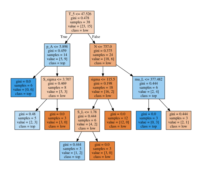
In order to infer the behavior of each method based on the datasets characteristics, we learn an interpretable meta-model using the features introduced in Table 1. While the metrics given in Table 1 are computed over entire datasets, then averaged over the corresponding collection, this experiment focuses on the training data and retains features for each of the 81 datasets. We use these features as input data, and fit one decision tree per algorithm in order to predict how a given method performs. The resulting models are binary classifiers where the target class is whether the average rank of the algorithm is among the top 25% performers (ranks 1 to 3), or if it reaches the lowest 25% (ranks 9 to 12). Figure 1 shows the trained meta-model of k-medoids-lev as an example. These trees expose the strengths and weaknesses of the methods studied, and highlight the most important factors impacting the methods’ performances.

Figure 1: Decision tree showing the position of k-medoids-lev in the overall ranking based on features extracted from the datasets. Ranks have been aggregated into the top and low classes which encompass the best (1 to 3) and worst (10 to 12) 25% ranks, respectively.

In order to provide a concise visual overview of this analysis, we report in Figure 2 the performance of each method based on the datasets’ characteristics. For this purpose, we extract the rules of the nodes for which $depth<4$ in all meta-models, then aggregate these rules per feature to identify values corresponding to the most important splits. The resulting filters are reported in the horizontal axis of the heatmap.

Figure 2: Novelty detection capabilities of the algorithms based on the datasets characteristics. The scores range from 0 to 10 and are based on the rank of the method averaged over the subset of datasets matching the corresponding filter applied to the 81 datasets. A score of 10 corresponds to an average rank of 1, while a score of 0 indicates that the method consistently ended in the last position. $N$ is the number of samples; $p_{A}$ is the proportion of anomalies; $M_{L}$, $\mu_{L}$ and $S_{L}$ are the minimum, average and entropy computed over the sequence length; $\sigma$ and $S_{\sigma}$ are the alphabet size and the corresponding entropy of its distribution, the entropy increasing with the number of events and the distribution uniformity; $T_{5}$ is the proportion of events represented by the 5% biggest events, a high value denotes important inequalities in the distribution; $L_{1}$ is the proportion of the smallest events representing 1% of the data, a high value indicates numerous events with rare occurrences; the genomics (gen), intrusion detection (int) and uba columns target datasets related to the corresponding field of study.

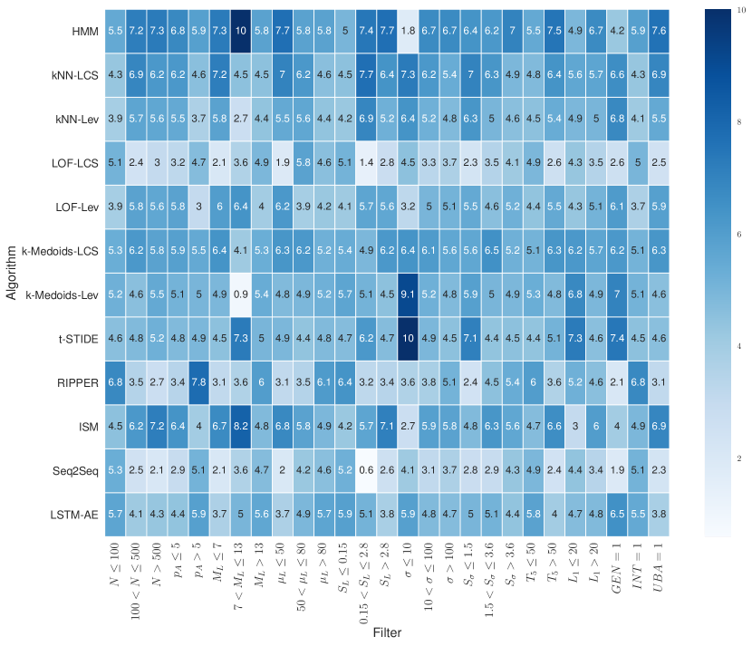
Our experiments show that no algorithm consistently reaches better results than the competing methods, but that hmm, k-nn and ism are promising novelty detection methods. While previous comparisonsstide1999intrusions ; chandola2008comparative ; Budalakoti2009airline use clean datasets exempt of anomalies, our study shows a good robustness for the selected methods, even for datasets with a high proportion of outliers, namely promoter, masquerade and intrusions.

Concerning the applications studied, k-nn, k-medoids, t-stide and lstm-ae show good performance on datasets related to genomics, which are splice-junctions, promoter and pfam. t-stide apart, these methods have successfully addressed numerous supervised numerical problems, and could thus reach good performance when applied to sequence-based supervised use cases. The best methods for intrusion detection are hmm and ripper, while t-stide shows reduced performance compared to stide1999intrusions , likely caused by the introduction of anomalies in the training sets. Our observations for genomics and intrusion detection corroborate the conclusions presented for t-stide and ripper in chandola2008comparative . However, our study shows much better performance for hmm, the previous study using a custom likelihood for hmm based on an aggregated sequence of binary scores. With regard to user behavior analysis, hmm, k-nn, k-medoids-lcs and ism show the best ability to differentiate users. While the performance of t-stide on uba is not sufficient to recommend the method, we believe that increasing the threshold of t-stide would lead to increased performance. Indeed, user actions are often based on well-defined application flows, and most of the possible subsequences are likely to exist in the training sets. The amount of supplementary information which can be provided by the models about the user behaviors will determine the most suitable methods for this field (Section 4.5).

Figure 2 shows that the performance of hmm improves significantly with the number of available samples. Both hmm and ism achieve good performance, even when a high discrepancy is observed among the sequence lengths. hmm, ism and ripper are able to handle efficiently a large alphabet of symbols. ripper also shows good performance for datasets containing a high proportion of outliers, while nearest neighbor methods are strongly impacted by this characteristic. Distance metrics are known to suffer from the curse of dimensionality inherent to a high number of features. Similarly, Figure 2 shows a decrease of performance for k-nn, k-medoids and lof when $\sigma$ increases, these methods relying on the lcs and Levenshtein metrics for distance computations. While lcs is a metric widely used in the literaturechandola2008comparative ; Budalakoti2009airline ; budalakoti2006anomaly , our experiments show that it does not perform better than the Levenshtein distance. If both lcs and the Levenshtein distance metrics provide satisfactory results for novelty detection when paired with k-nn or k-medoids, the combination of lof and lcs produces the lowest accuracy of our evaluation. Nonetheless, the efficiency of lof-lev prevents us from discarding this method, even though k-nn-lev achieves a similar accuracy to lof-lev with a simpler scoring function. For the sake of the experiment, we evaluated the scoring function proposed for t-stide in hofmeyr1998intrusion . For each subsequence of fixed length in a test sequence, the authors compute the hamming distance between the test window and all training windows, and return the shortest distance. This method was much slower than a binary decision based on the presence of the test window in the training set, and did not strongly improve the results. Neural networks do not stand out in this test. The reconstruction error showed good results for detecting numerical anomalies in previous studiessakurada2014anomaly ; Marchi2015denoising , but the approach may not be appropriate for event sequences. The reconstructed sequences provided by seq2seq are often longer than the input data, and the network loops regularly for a while over a given event. Figure 2 show that lstm networks perform better with long sequences and a moderate alphabet size. We repeated our experiments using the Python library difflib as an alternative to lcs for seq2seq, but it did not improve the performance of the network. lstm-ae shows an acceptable novelty detection accuracy, which could be further improved with dropout and attention. Thanks to their moderate depth, these two networks do not require very large datasets to tune their parameters. For example, lstm-ae achieves a good map even for small datasets such as promoter and masquerade. Despite the use of masks to address padding, these methods have difficulty with datasets showing an important disparity in sequence length, such as intrusions and the four collections of uba datasets.

4.2 Robustness

Figures 3 to 5 report the mean area under the precision recall curve (map) for datasets of increasing proportion of outliers, number of samples and sequence length, respectively. The positive class represents the nominal samples in Figure 3, and the anomalies in Figure 4 and 5 (as in Section 4.1).

Figure 3: Robustness for increasing noise density

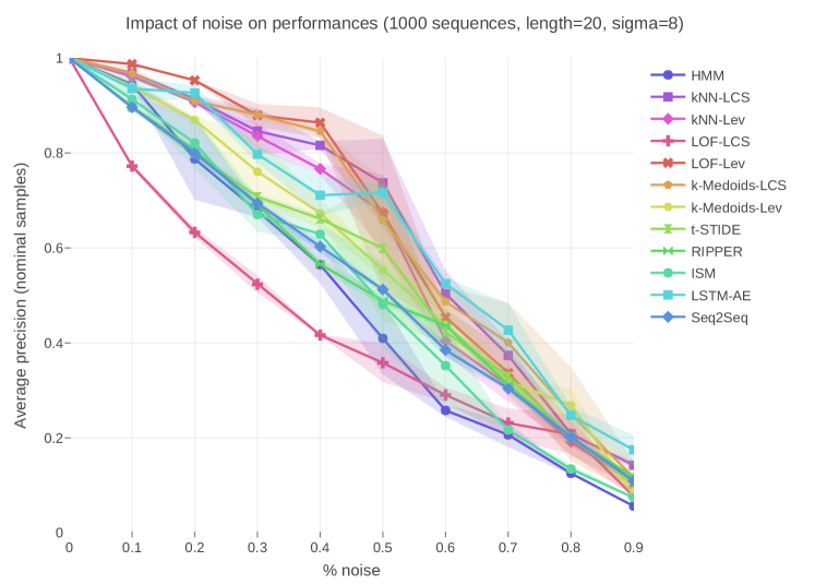
Figure 3 demonstrates a more complex test case than just identifying uniform background noise against a well-defined distribution. In this test, anomalies are sampled according to their own probability distribution, which will affect the models learnt when a sufficient proportion of anomalies is reached. The test highlights thus how algorithms deal with complex data based on multiple distributions. We observe that most algorithms focus on the major distribution as long as the proportion of corresponding samples remains higher than 60%. hmm uses 3 components and may thus learn the second distribution much earlier in the test. On the opposite, most of the distance-based methods discard the smallest distribution even if this one represents up to 40% of the data. lof-lcs shows poor performance from the very beginning, which prevents us from concluding on the behavior of this method.

Figure 4: Robustness for increasing number of samples

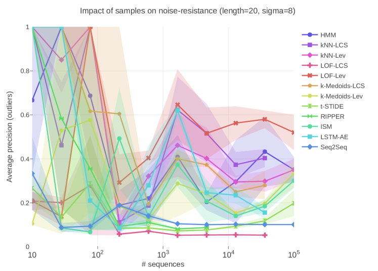
Figure 4 shows that 200 samples are a good basis to reach stable novelty detection results. While we expected the performance of deep learning methods to improve with the number of samples, these networks did not significantly increase their detection with the size of the dataset. The best results on large datasets were achieved by distance-based methods, most of which rely on nearest-neighbor approaches particularly efficient when a high number of samples is available. Good performance were also achieved by hmm, presumably due to a generation method for nominal samples and outliers based on Markov chains, which matches the internal representation of hmm.

Figure 5: Robustness for increasing sequence length

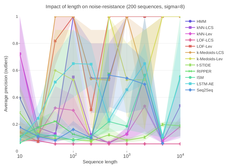
Despite the increasing volume of data over the scalability test reported in Figure 5, important variations can be observed for the results, e.g. for a length of 200 events. Such variations are probably related to the limited number of samples used in the generated datasets, which is a computational requirement to perform experiments with long sequences for several algorithms. k-medoids achieve better performance than other distance-based methods, which suggests a better approach for small datasets. hmm achieves once again good results, while lstm networks show improved novelty detection capabilities for datasets containing sequences longer than 100 events. The performance of ism also increases with the volume of data, although the method require bigger datasets to reach comparable results.

In summary, our experiments show that robust models require at least 200 training samples to provide satisfactory results. lof-lcs and t-stide do not provide satisfactory performance, even though fine-tuning t-stide by increasing the frequency threshold could lead to better results.

4.3 Runtime performance

The computation time for training and prediction steps is reported in Figures 6 to 9. While time measurements are impacted by hardware configuration (Sec. 3.2), the slope of the curves and their ranking compared to other methods should remain the same for most running environments.

Figure 6: Training time for increasing number of samples

Figure 7: Prediction time for increasing number of test samples

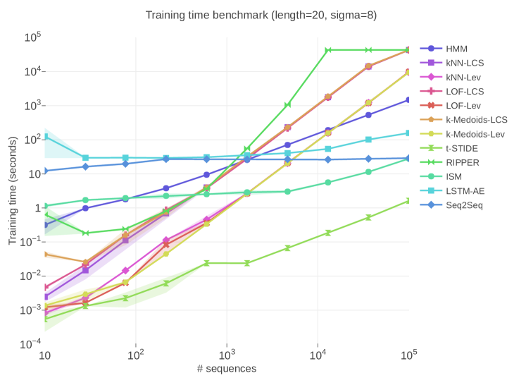
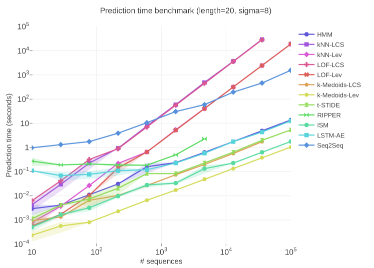
The measurements from Figures 6 and 7 show a poor scalability of algorithms relying on pairwise distance matrices, namely lof, k-nn and k-medoids. Most of the training and prediction time of these methods is dedicated to the computation of the distance matrix, and thus to the lcs and Levenshtein algorithms. Since training and testing sets have the same number of samples in this test, the previous assumption is confirmed by observing a similar training and prediction time for the methods. In addition, k-medoids is the only distance-based algorithm with a faster prediction time, caused by a smaller number of distances to compute. The prediction step of this method requires only to compare a small number of medoids with the testing set, instead of performing a heavy pairwise comparison. Regarding distance metrics, lcs shows a much higher computation time than the Levenshtein distance despite a similar time complexity. The resort to alternative and faster implementationscrochemore2003speedinglcs; hunt1977fastlcs is thus recommended. Furthermore, parallel or distributed algorithms could be used for pairwise distance matrix computations, which would significantly reduce the computation time of these methodschang2008pairwise. However, distance-based methods would likely remain among the most computationally expensive algorithms when applied to a high number of observations. Despite a very small $\sigma$, the rule-learning algorithm ripper shows the highest training time, reaching our 12-hour timeout for 13,000 samples. The missing results for the prediction step (Fig. 7) are thus caused by an interrupted training. On the opposite and as expected, the use of mini-batch learning by lstm-ae and seq2seq allows the two methods to efficiently handle the increasing number of sequences, although we recommend to increase the batch size or the number of iterations according to the size of the training set. However, such technique is only valid for the training step, and both methods show a scoring scalability comparable to the other algorithms. The extreme simplicity of t-stide, which essentially stores subsequences in a dictionary at train time, makes this algorithm one of the fastest methods. The increasing load does not affect much ism, since the method stops iterating over the dataset if it does not find new interesting patterns after a given number of sequences.

Figure 8: Training time for increasing sequence length

Figure 9: Prediction time for increasing sequence length

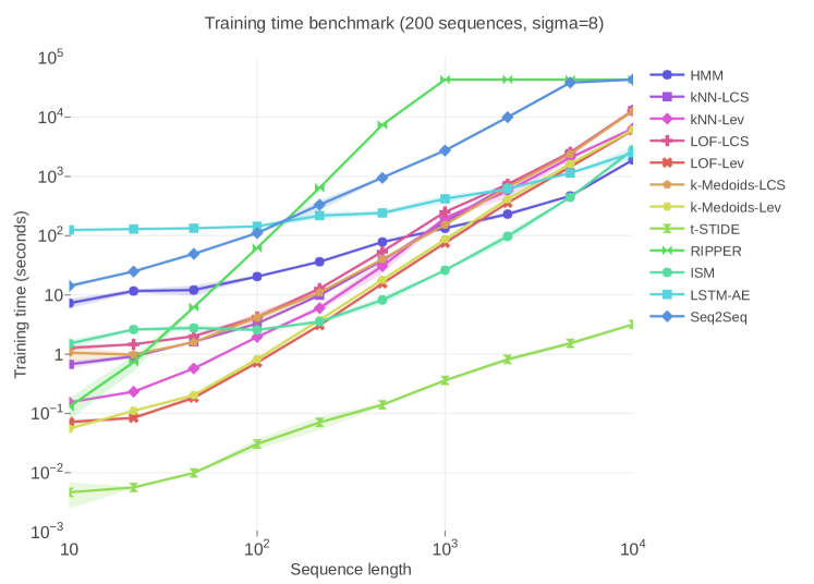
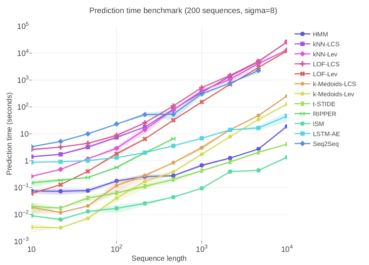
We now use a fixed number of samples while increasing the length of the sequences and report the computation time in Figures 8 and 9. The careful reader will notice that both scalability tests, i.e. number of sequence-based and length-based, produce datasets containing the exact same number of symbols (e.g. $10^{5}\ sequences*20\ symbols=200\ sequences*10^{4}\ symbols$). This configuration reveals the true impact of samples and length on the scalability, while keeping the same volume of data. While we still observe a poor scalability for distance-based algorithms caused by a high computation time to compute distances, the training and prediction time of these methods was reduced due to a smaller number of samples to handle by the core algorithm. On the opposite, ripper and ism show a much higher training time when dealing with long sequences. However, the prediction time of these two methods only depends on the volume of data, i.e. the total number of symbols in the dataset, and will be impacted similarly by the number of samples and length. Mini-batch methods are now subject to training batches of increasing volume, which reveals a poor scalability for seq2seq. lstm-ae performs better due to an early stopping mechanism, interrupting the training when the loss does not improve sufficiently over the iterations. The computation time of these two neural networks could however be improved with the use of dedicated GPU architectures. These tests show the limitations of ripper, which suffers from a long training step, even for datasets of reasonable size. Distance-based methods and seq2seq also show limited scalability, although k-medoids provide fast predictions and seq2seq easily supports datasets containing a large number of samples. ism and t-stide show the best computation time for both training and prediction steps, and could even prove useful in lightweight applications.

4.4 Memory usage

Monitoring the memory consumption in Figures 10 and 11 highlights important scalability constraints for several algorithms.

Figure 10: Memory usage for increasing number of samples

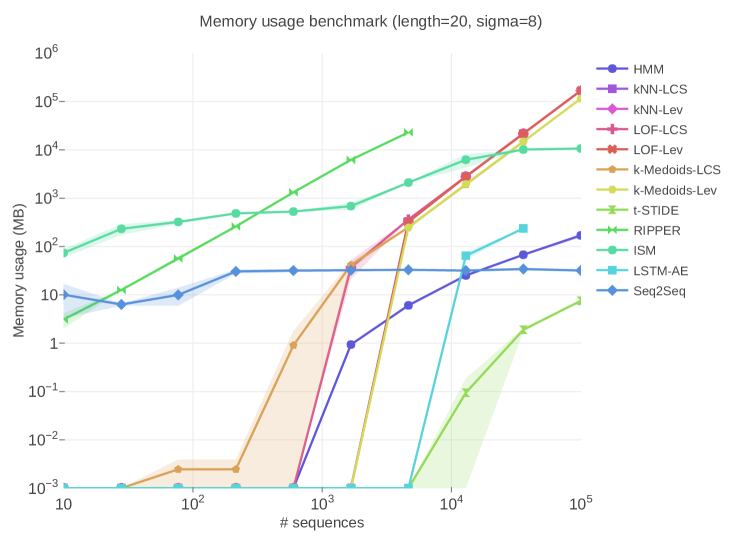
We first observe in Figure 10 that memory usage for ripper and distance-based methods is strongly correlated with the number of input sequences. ripper shows a very high memory usage, although the method reaches our 12h timeout at train time before exceeding the limit of 256GB RAM. Distance-based methods are also strongly impacted by the number of samples. However, most of the memory is here consumed by the pairwise distance matrix. Despite storage optimizations, e.g. symmetric matrix, integers are stored on 24 bytes by Python, resulting in a memory usage of 114GB and 167GB for k-nn-lev and lof-lev, respectively. Interestingly, ism stabilizes at 10GB after having discovered a sufficient number of patterns from the data. Mini-batch neural networks are not strongly impacted by the number of samples, and the small $\sigma$ limits the diversity of sequences, thus reducing the memory usage of t-stide.

Figure 11: Memory usage for increasing sequence length

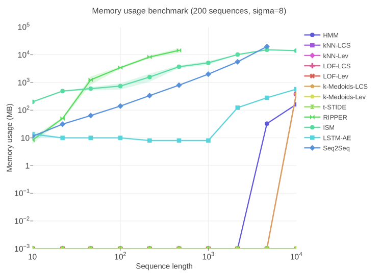
The metrics reported in Figure 11 corroborate the previous conclusions. The experiment reveals a number of rules learnt by ripper increasing linearly with the number of events, the final model containing in average $\frac{\#events}{50}$ rules. The size of the decision tree built by association rule learning is thus correlated with the volume of the data. To the opposite, the memory usage of ISM stabilizes again after convergence, showing a more efficient internal representation of the data than ripper. The memory consumption of distance-based methods is very low due to small distance matrices, although the computation of lcs shows a memory usage increasing with the length of the sequences compared. Neural networks, especially seq2seq, are more impacted by the increasing sequence length. This is caused by a network topology depending on the size of the padded sequences, in addition to matrix multiplications of dimensionalities directly impacted by the length of the sequences.

We have observed that most algorithms have a memory consumption strongly related to the volume of input data. The requirements of ripper are too important for most systems, and distance-based methods are not suitable to address problems pertaining to more than 20,000 sequences. Interestingly, we did not observe correlations between training or prediction time and memory usage, while one could expect fast algorithms consume more memory, performing faster computations due to a massive caching system. If this may be true when comparing similar methods, the important differences in time and memory are here caused by major discrepancies in the approaches taken by the algorithms.

4.5 Interpretability

The ability for humans to understand a machine learning model and the resulting predictions is called interpretability. This trait allows data scientists to validate the final model and provides useful insights on the targeted dataset, e.g. discovering valuable information about user behaviors which have an important business value. While continuous scores are usually sufficient for automatic intervention modules, this information and the corresponding ranking may not be sufficient when a manual investigation of the anomalies is required. This situation arises for critical applications, where false positives could strongly impact the brand image, e.g. deny access to services for a business partner, or incur heavy costs, e.g. component replacement based on failure prediction with applications to data centers and airplanes. In this case, especially if many alerts are raised every day, the time allocated to manual investigation could be greatly reduced if we could provide the motivations behind high scores to the human expert. Transparency is thus an essential criterion for the choice of algorithms in many applications, and data analysts may accept to trade performance for model accountability. If human eyes may differentiate outlying activity from the underlying patterns in numerical time-series, this task is much harder for discrete event sequences, which emphasizes the need for model interpretability.

The internal representation of interpretable methods provides sufficient information to motivate a predicted score with respect to an input sequence. For example, hmm learns intuitive transition and emission matrices, providing an insightful weighted process flowchart. Unusual event transitions in the test sequence can be visually highlighted by putting a threshold on the emission transition probabilities. Pairwise distance matrices also convey valuable information and can be turned into intuitive visualizations. The matrices can be plotted as Voronoi diagrams, heat maps or fed into a multidimensional scaling (MDS) algorithm resulting in a scatter plot of chosen dimensionality. If additional insight on the distance computations is required, lcs is an intuitive metric and the subsequence common to two compared samples can be underlined. On the other hand, the cost matrix computed by Levenshtein is more difficult to read. Further on, the scoring performed by distance-based methods can be easily motived in the previous 2D representations of distance matrices, e.g. by highlighting the test sample and its $k^{th}$ neighbor for k-nn, or the corresponding medoid for k-medoids. The scoring function of lof is more complex, as it studies the local density of a test sample and its neighbors. Moving back to standard sequence representations, t-stide is extremely accountable and subsequences can be underlined based on their frequency in the model, thus motivating the resulting score. Pointing out events incorrectly predicted by ripper should also provide some information, and interesting patterns learnt by ism could be emphasized similarly. Neural networks are closer to black-box systems, and their interpretability has recently gained a lot of attention Zhang2018interpretability . However, recent efforts mostly focus on numerical and convolutional networks, which leaves room for future lstm representations. Differences between the input sequence and the reconstructed output could be highlighted for seq2seq, although it would not explain the underlying model. For lstm-ae, we could learn and plot a low dimensional numerical representation based on the internal representation of the network, but dimensionality reduction methods will often produce an output biased towards the average sample of the dataset onderwater2015outlier and must be selected with care. This is the reason why the reconstruction error is used with seq2seq to identify anomalies.

In order to overcome the lack of accountability of a given algorithm, an alternative approach is to infer meaningful rules based on the inputs and outputs predicted by a trained modelfortuny2015extraction . The rule extraction method should provide simple rules showing a transparent decision, while minimizing the prediction error. This is a popular approach used to improve the interpretability of classification models, in particular neural networks and support vector machines (svms). Two good rule extraction methods for classifiers are osreetchells2006extraction and hypinvsaad2009inversion . These methods are also compatible with novelty detection when the targeted model produces a binary output such as fraud and non-fraud. If a continuous anomaly score is required to rank anomalies, we should then resort to regression rule extraction methods which learn rules producing a continuous output, e.g. REFANNsetiono2002extraction , ITERhuysmans2006extraction or classification and regression trees (cart)breiman2017cart . Both regression and classification rule mining methods show good performance when applied to numerical or one-hot encoded input data. In order to feed temporal data to these algorithms (or to any standard regression or classification methods), numerical features should be extracted from the sequences during a preprocessing step. The feature selection must be performed with great care to minimize the amount of information lost, and was automated for continuous time-series in a previous workchrist2016distributed . While different features should be selected for discrete event sequences, either manually or based on existing techniqueswang2001feature ; saidi2010feature , any regression rule extraction technique can be subsequently applied for both data types. The numerical latent representation provided by lstm autoencoders could be used as input features for rule mining, but it would only improve the interpretability of the decoder, leaving aside the data transformation performed by the encoder. Table 4 summarizes our observations about the scalability and interpretability of the methods surveyed.

Table 4: Scalability and interpretability summary. Runtime and memory consumption are reported for synthetic datasets of increasing number of samples and sequence length.

	Training/prediction time		Mem. usage
Algorithm	$\mathrel{\text{\rotatebox[origin={c}]{45.0}{$\vrule height=0.0pt,width=0.0pt\rightarrow$}}}$ Samples	$\mathrel{\text{\rotatebox[origin={c}]{45.0}{$\vrule height=0.0pt,width=0.0pt\rightarrow$}}}$ Length	$\mathrel{\text{\rotatebox[origin={c}]{45.0}{$\vrule height=0.0pt,width=0.0pt\rightarrow$}}}$ Samples	$\mathrel{\text{\rotatebox[origin={c}]{45.0}{$\vrule height=0.0pt,width=0.0pt\rightarrow$}}}$ Length	Interpretability
hmm	Medium/Low	Low/Low	Low	Low	High
k-nn-lcs	High/High	Medium/High	High	Low	High
k-nn-lev	High/High	Medium/High	High	Low	Medium
lof-lcs	High/High	Medium/High	High	Low	Medium
lof-lev	High/High	Medium/High	High	Low	Medium
k-medoids-lcs	High/Low	Medium/Medium	High	Low	High
k-medoids-lev	High/Low	Medium/Medium	High	Low	Medium
t-stide	Low/Low	Low/Low	Low	Low	High
ripper	High/Low	High/Medium	High	High	Medium
ism	Low/Low	Medium/Low	Medium	Medium	High
seq2seq	Low/Medium	High/High	Low	High	Low
lstm-ae	Low/Low	Low/Low	Low	Medium	Low

5 Conclusions

This work studied the performance and scalability of state-of-the-art novelty detection methods based on a significant collection of real and synthetic datasets. The standard metric used in the literature to compare event sequences is lcs. Given the evidence provided, we found that although lcs produced more transparent insights than the Levenshtein distance, it did not exhibit better anomalies and was computationally more expensive. Our experiments suggest that k-nn, k-medoids, t-stide and lstm-ae are suitable choices to identify outliers in genomics, and that hmm and ripper are efficient algorithms to detect intrusions. hmm is a strong candidate for most novelty detection applications, and shows a good scalability and interpretability. These characteristics make hmm appropriate for user behavior analysis, along with k-nn, k-medoids and ism which also provide a good model accountability. The fast scoring achieved by hmm, t-stide and ism implies an excellent management of heavy loads arising in production environments. Major scalability constraints are pointed out for ripper and distance-based methods, namely k-nn, k-medoids and lof. The resort to alternative approaches when tackling large volumes of data is recommended. The widely used lstm networks show a lack of interpretability, and we believe that improving the understanding of recurrent networks as performed in Karpathy2016 would strongly benefit to the research community. Most approaches evaluated in this study are suitable for supervised tasks based on event sequences. Studying how these methods compare in a supervised context would be of interest.

6 Acknowledgments

The authors wish to thank the Amadeus Middleware Fraud Detection team directed by Virginie Amar and Jérémie Barlet, led by the product owner Christophe Allexandre and composed of Jean-Blas Imbert, Jiang Wu, Yang Pu and Damien Fontanes for building the rights, transactions-fr and transactions-mo datasets. MF gratefully acknowledges support from the AXA Research Fund.

References

- [1] C. C. Aggarwal. Outlier Analysis, pages 237–263. Springer International Publishing, Cham, 2015.
- [2] L. Bergroth, H. Hakonen, and T. Raita. A survey of longest common subsequence algorithms. In Proceedings Seventh International Symposium on String Processing and Information Retrieval. SPIRE 2000, pages 39–48, 2000.
- [3] L. Breiman, J. Friedman, R. Olsen, and C. Stone. Classification and regression trees. Wadsworth and Brooks, 1984.
- [4] M. M. Breunig, H.-P. Kriegel, R. T. Ng, and J. Sander. LOF: Identifying density-based local outliers. SIGMOD Record, 29(2):93–104, May 2000.
- [5] S. Budalakoti, A. N. Srivastava, R. Akella, and E. Turkov. Anomaly detection in large sets of high-dimensional symbol sequences. Technical Report NASA TM-2006-214553, 2006.
- [6] S. Budalakoti, A. N. Srivastava, and M. E. Otey. Anomaly detection and diagnosis algorithms for discrete symbol sequences with applications to airline safety. IEEE Transactions on Systems, Man, and Cybernetics, Part C (Applications and Reviews), 39(1):101–113, Jan 2009.
- [7] V. Chandola, A. Banerjee, and V. Kumar. Anomaly detection for discrete sequences: A survey. IEEE Transactions on Knowledge and Data Engineering, 24(5):823–839, May 2012.
- [8] V. Chandola, V. Mithal, and V. Kumar. Comparative evaluation of anomaly detection techniques for sequence data. In 2008 Eighth IEEE International Conference on Data Mining, pages 743–748, Dec 2008.
- [9] M. Christ, A. W. Kempa-Liehr, and M. Feindt. Distributed and parallel time series feature extraction for industrial big data applications. arXiv preprint arXiv:1610.07717, 2016.
- [10] W. W. Cohen. Fast effective rule induction. In A. Prieditis and S. Russell, editors, Machine Learning Proceedings 1995, pages 115 – 123. Morgan Kaufmann, San Francisco (CA), 1995.
- [11] J. Davis and M. Goadrich. The relationship between precision-recall and roc curves. In Proceedings of the 23rd international conference on Machine learning, pages 233–240. ACM, 2006.
- [12] E. J. de Fortuny and D. Martens. Active learning-based pedagogical rule extraction. IEEE Transactions on Neural Networks and Learning Systems, 26(11):2664–2677, Nov 2015.
- [13] R. Domingues, P. Michiardi, J. Zouaoui, and M. Filippone. Deep gaussian process autoencoders for novelty detection. Machine Learning, Jun 2018.
- [14] A. Emmott, S. Das, T. Dietterich, A. Fern, and W.-K. Wong. A meta-analysis of the anomaly detection problem. arXiv preprint arXiv:1503.01158v2, 2016.
- [15] T. A. Etchells and P. J. G. Lisboa. Orthogonal search-based rule extraction (osre) for trained neural networks: a practical and efficient approach. IEEE Transactions on Neural Networks, 17(2):374–384, March 2006.
- [16] J. Fowkes and C. Sutton. A subsequence interleaving model for sequential pattern mining. In Proceedings of the 22Nd ACM SIGKDD International Conference on Knowledge Discovery and Data Mining, KDD ’16, pages 835–844, New York, NY, USA, 2016. ACM.
- [17] W. Gan, J. C.-W. Lin, P. Fournier-Viger, H.-C. Chao, and P. S. Yu. A survey of parallel sequential pattern mining. arXiv preprint arXiv:1805.10515, 2018.
- [18] S. García, A. Fernández, J. Luengo, and F. Herrera. Advanced nonparametric tests for multiple comparisons in the design of experiments in computational intelligence and data mining: Experimental analysis of power. Information Sciences, 180(10):2044 – 2064, 2010. Special Issue on Intelligent Distributed Information Systems.
- [19] M. Gupta, J. Gao, C. C. Aggarwal, and J. Han. Outlier detection for temporal data: A survey. IEEE Transactions on Knowledge and Data Engineering, 26(9):2250–2267, Sept 2014.
- [20] S. Hochreiter and J. Schmidhuber. Long short-term memory. Neural computation, 9(8):1735–1780, 1997.
- [21] V. Hodge and J. Austin. A survey of outlier detection methodologies. Artificial Intelligence Review, 22(2):85–126, Oct 2004.
- [22] S. A. Hofmeyr, S. Forrest, and A. Somayaji. Intrusion detection using sequences of system calls. Journal of computer security, 6(3):151–180, 1998.
- [23] J. Huysmans, B. Baesens, and J. Vanthienen. Iter: An algorithm for predictive regression rule extraction. In A. M. Tjoa and J. Trujillo, editors, Data Warehousing and Knowledge Discovery, pages 270–279, Berlin, Heidelberg, 2006. Springer Berlin Heidelberg.
- [24] A. Karpathy, J. Johnson, and F. Li. Visualizing and Understanding Recurrent Networks. In Proceedings of the Fourth International Conference on Learning Representations (ICLR 2016), May 2016.
- [25] Z. W. Kundzewicz and A. J. Robson. Change detection in hydrological records - a review of the methodology. Hydrological Sciences Journal, 49(1):7–19, 2004.
- [26] A. Lazarevic, L. Ertoz, V. Kumar, A. Ozgur, and J. Srivastava. A comparative study of anomaly detection schemes in network intrusion detection. In Proceedings of the 2003 SIAM International Conference on Data Mining, pages 25–36, 2003.
- [27] W. Lee, S. J. Stolfo, and P. K. Chan. Learning patterns from unix process execution traces for intrusion detection. In AAAI Workshop on AI Approaches to Fraud Detection and Risk Management, pages 50–56, 1997.
- [28] V. I. Levenshtein. Binary Codes Capable of Correcting Deletions, Insertions and Reversals. Soviet Physics Doklady, 10:707, Feb. 1966.
- [29] Z. C. Lipton, J. Berkowitz, and C. Elkan. A Critical Review of Recurrent Neural Networks for Sequence Learning. ArXiv e-prints, May 2015.
- [30] F. T. Liu, K. M. Ting, and Z.-H. Zhou. Isolation forest. In Proceedings of the 2008 Eighth IEEE International Conference on Data Mining, ICDM ’08, pages 413–422. IEEE Computer Society, 2008.
- [31] M.-T. Luong, H. Pham, and C. D. Manning. Effective approaches to attention-based neural machine translation. arXiv preprint arXiv:1508.04025, 2015.
- [32] E. Marchi, F. Vesperini, F. Eyben, S. Squartini, and B. Schuller. A novel approach for automatic acoustic novelty detection using a denoising autoencoder with bidirectional lstm neural networks. In 2015 IEEE International Conference on Acoustics, Speech and Signal Processing (ICASSP), pages 1996–2000, April 2015.
- [33] R. A. Maxion and T. N. Townsend. Masquerade detection using truncated command lines. In Proceedings International Conference on Dependable Systems and Networks, pages 219–228, 2002.
- [34] M. Onderwater. Outlier preservation by dimensionality reduction techniques. International Journal of Data Analysis Techniques and Strategies, 7(3):231–252, 2015.
- [35] H.-S. Park and C.-H. Jun. A simple and fast algorithm for k-medoids clustering. Expert Systems with Applications, 36(2, Part 2):3336 – 3341, 2009.
- [36] S. Petrović, M. Osborne, and V. Lavrenko. Streaming first story detection with application to twitter. In Human Language Technologies: The 2010 Annual Conference of the North American Chapter of the Association for Computational Linguistics, HLT ’10, pages 181–189, Stroudsburg, PA, USA, 2010. Association for Computational Linguistics.
- [37] V. Pihur, S. Datta, and S. Datta. RankAggreg, an r package for weighted rank aggregation. BMC Bioinformatics, 10(1):62, Feb 2009.
- [38] L. R. Rabiner. A tutorial on hidden markov models and selected applications in speech recognition. Proceedings of the IEEE, 77(2):257–286, Feb 1989.
- [39] S. Ramaswamy, R. Rastogi, and K. Shim. Efficient algorithms for mining outliers from large data sets. In Proceedings of the 2000 ACM SIGMOD International Conference on Management of Data, SIGMOD ’00, pages 427–438, New York, NY, USA, 2000. ACM.
- [40] E. W. Saad and D. C. Wunsch. Neural network explanation using inversion. Neural Networks, 20(1):78 – 93, 2007.
- [41] R. Saidi, M. Maddouri, and E. Mephu Nguifo. Protein sequences classification by means of feature extraction with substitution matrices. BMC Bioinformatics, 11(1):175, Apr 2010.
- [42] M. Sakurada and T. Yairi. Anomaly detection using autoencoders with nonlinear dimensionality reduction. In Proceedings of the MLSDA 2014 2nd Workshop on Machine Learning for Sensory Data Analysis, pages 4–11. ACM, 12 2014.
- [43] D. Sculley and C. E. Brodley. Compression and machine learning: a new perspective on feature space vectors. In Data Compression Conference (DCC’06), pages 332–341, March 2006.
- [44] R. Setiono, W. K. Leow, and J. M. Zurada. Extraction of rules from artificial neural networks for nonlinear regression. IEEE Transactions on Neural Networks, 13(3):564–577, May 2002.
- [45] P. Sun, S. Chawla, and B. Arunasalam. Mining for outliers in sequential databases. In Proceedings of the 2006 SIAM International Conference on Data Mining, pages 94–105, 2006.
- [46] I. Sutskever, O. Vinyals, and Q. V. Le. Sequence to sequence learning with neural networks. In Z. Ghahramani, M. Welling, C. Cortes, N. D. Lawrence, and K. Q. Weinberger, editors, Advances in Neural Information Processing Systems 27, pages 3104–3112. Curran Associates, Inc., 2014.
- [47] S. J. Taylor and B. Letham. Forecasting at scale. The American Statistician, 72(1):37–45, 2018.
- [48] J. T. L. Wang, Q. Ma, D. Shasha, and C. H. Wu. New techniques for extracting features from protein sequences. IBM Systems Journal, 40(2):426–441, 2001.
- [49] C. Warrender, S. Forrest, and B. Pearlmutter. Detecting intrusions using system calls: alternative data models. In Proceedings of the 1999 IEEE Symposium on Security and Privacy (Cat. No.99CB36344), pages 133–145, 1999.
- [50] Q.-s. Zhang and S.-c. Zhu. Visual interpretability for deep learning: a survey. Frontiers of Information Technology & Electronic Engineering, 19(1):27–39, Jan 2018.