Rank–2 $U(1)$ spin liquid on the breathing pyrochlore lattice

Abstract

Higher–rank generalisations of electrodynamics have recently attracted considerable attention because of their ability to host “fracton” excitations, with connections to both fracton topological order and gravity. However, the search for higher–rank gauge theories in experiment has been greatly hindered by the lack of materially–relevant microscopic models. Here we show how a spin liquid described by rank–2 $U(1)$ gauge theory can arise in a magnet on the breathing pyrochlore lattice. We identify Yb–based breathing pyrochlores as candidate systems, and make explicit predictions for how the rank–2 $U(1)$ spin liquid would manifest itself in experiment.

Introduction. It is of great intellectual interest and practical utility to discover novel effective laws of nature emerging from many–body systems. Traditionally, this enterprise has been entwined with the concept of broken symmetry Anderson (1972). However, a powerful alternative has proved to be the local constraints which arise from competing or “frustrated”, interactions. In the context of frustrated magnets, these can lead to the emergence of a local gauge symmetry, and thereby to quantum spin liquids, which defy all usual concepts of magnetic order, and instead exhibit fractionalised excitations and long–range entanglement Anderson (1973); Balents (2010); Savary and Balents (2017); Zhou et al. (2017). A well–studied example is quantum spin ice, a realisation of a $U(1)$ gauge theory on the pyrochlore lattice, whose emergent excitations exactly mimic conventional electrodynamics: photons, electric charges and magnetic monopoles. As such, it has attracted intense theoretical Hermele et al. (2004); Banerjee et al. (2008); Benton et al. (2012); Savary and Balents (2012); Shannon et al. (2012); Hao et al. (2014); Gingras and McClarty (2014); Kato and Onoda (2015); Chen (2017); Huang et al. (2018) and experimental Zhou et al. (2008); Ross et al. (2011); Fennell et al. (2012); Kimura et al. (2013); Sibille et al. (2015); Wen et al. (2017); Thompson et al. (2017); Sibille et al. (2018); Gao et al. (2019) investigation.

Recent work has highlighted the possibility of more exotic forms of emergent electrodynamics Xu (2006); Pretko (2017a); Rasmussen et al. (2016); Pretko (2017b), where electric and magnetic fields have the form of rank–2 (or higher–rank) tensors. These theories have modified conservation laws and gauge symmetries, resulting in some remarkable properties. Some are argued to mimic gravity Xu (2006); Benton et al. (2016); Pretko (2017c), while others are dual to elasticity theory Pretko and Radzihovsky (2018); Gromov (2019). In both cases, the charged excitations, dubbed “fractons”, have constrained mobility, and characterize a new class of topological order Chamon (2005); Shannon et al. (2004); Haah (2011); Vijay et al. (2015, 2016); Bulmash and Barkeshli (2018); Ma et al. (2018); Nandkishore and Hermele (2019); Slagle and Kim (2017); Halász et al. (2017a). Fracton models are also linked to quantum stabilizer codes Schmitz et al. (2018); Kubica and Yoshida (1836) and holography Yan (2019). None the less, these desirable properties come at a price: the local constraint required has a tensor character. As a consequence, prototypical models of fractons require rather complicated interactions Chamon (2005); Xu (2006); Haah (2011); Vijay et al. (2015, 2016), with just a handful of proposals motivated by experiment Slagle and Kim (2017); Halász et al. (2017b); You and von Oppen (2019). In the case of gapless higher–rank gauge theories, only a few concrete models exist Xu and Hořava (2010); Xu and Fisher (2007); Rasmussen et al. (2016), and even less is known about how to achieve such a phase in a real material. For this reason, realizing an emergent higher–rank electrodynamics in experiment presents a significant challenge.

(a) BP Lattice

(b) 0kl plane

(c) hk0 plane

(d) $\langle E_{\sf xy}({\bf q})E_{\sf xy}(-{\bf q})\rangle$

Figure 1: Breathing pyrochlore (BP) lattice, and singular correlations characteristic of a rank–2 $U(1)$ [R2–U1] gauge theory. (a) BP lattice, with A– and B–sublattice tetrahedra of unequal size. The vectors associated with Dzyaloshinskii–Moriya (DM) interactions on the A–sublattice [Eq. (6)] are illustrated with green arrows. (b) Prediction of R2–U1 theory for the correlation function $\langle E_{\sf xy}({\bf q})E_{\sf xy}({\bf-q})\rangle$ [Eq. (17)], showing a 2–fold pinch point in the [0kl] plane. (c) Perpendicular section, showing a 4–fold pinch point (4FPP) in the [hk0] plane. (d) Equivalent results from MC simulation of the breathing pyrochlore model [Eq. (6)].

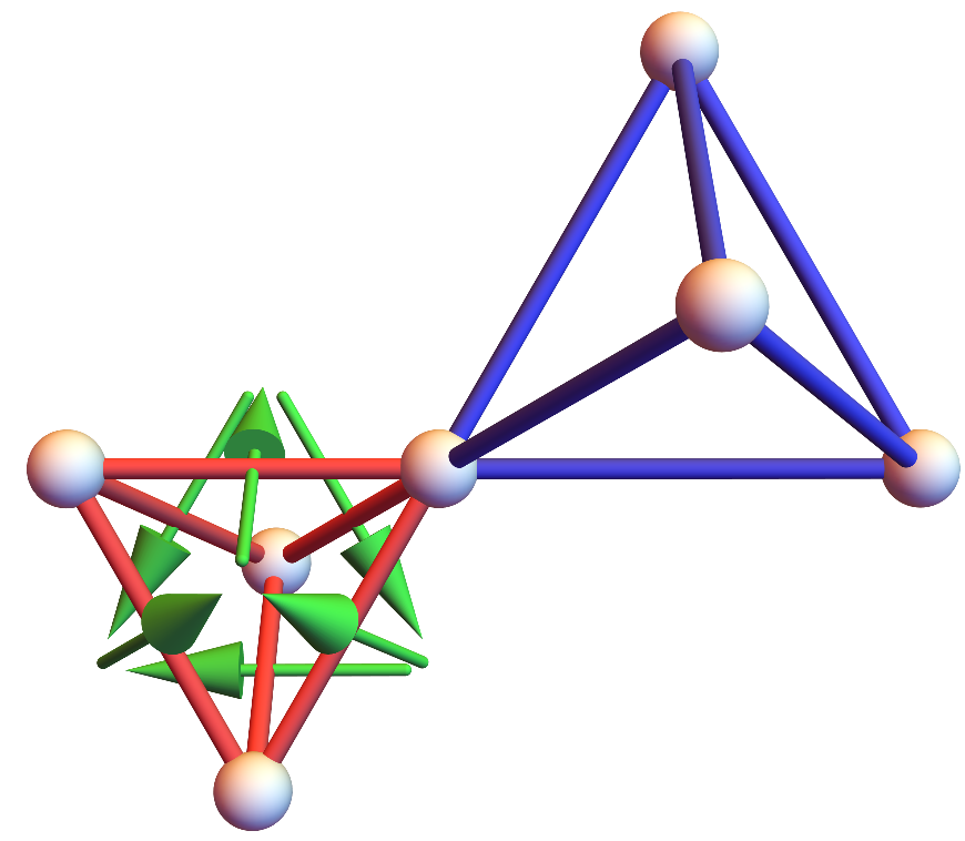
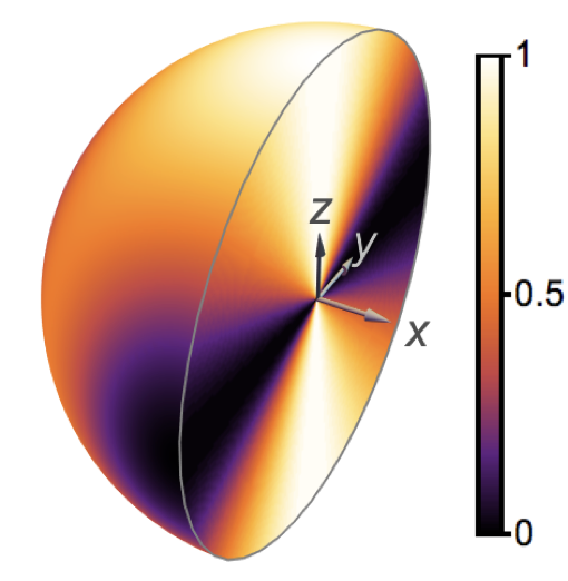
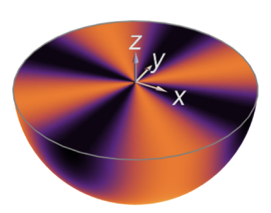
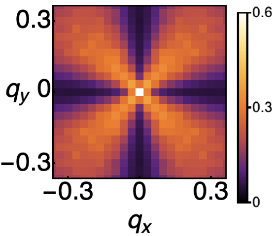
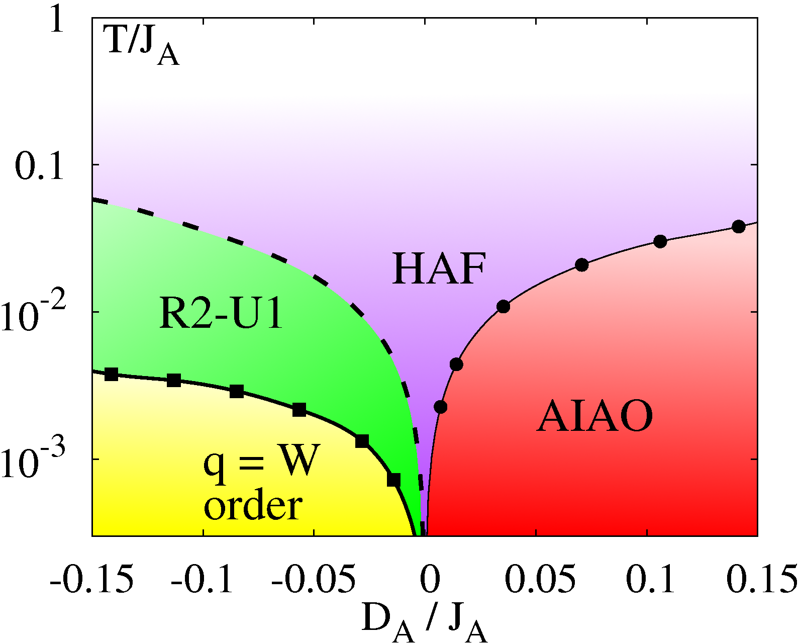
In this Letter we show how a canonical rank–2 $U(1)$ [R2–U1] spin liquid can arise in a realistic model of a frustrated magnet. The model we consider is the Heisenberg antiferromagnet (HAF) on a breathing–pyrochlore (BP) lattice, perturbed by weak Dzyaloshinskii–Moriya (DM) interactions [Fig. 1a]. Working in the classical limit, relevant to a spin liquid at finite temperatures, we establish that fluctuations can be described using a tensor field satisfying the constraints required for a R2–U1 gauge theory. We use classical Monte Carlo (MC) simulation to confirm this scenario, and to explore how a R2–U1 spin liquid could be identified in experiment. We find that 4–fold pinch points (4FPP), characteristic of the R2–U1 state Prem et al. (2018), become visible in polarised neutron scattering. We discuss the application of these ideas to real materials, identifying Yb–based breathing pyrochlores as potential candidates for an R2–U1 spin liquid state. These results complement earlier work exploring gapped, fracton topological order, in models with bilinear interactions Slagle and Kim (2017); Halász et al. (2017b); You and von Oppen (2019), providing an example of an R2–U1 state, in an experimentally–motivated context.

Review of R2–U1 theory. Conventional, $U(1)$, electrodynamics is built around a vector field $\bf E$, subject to a Gauss law $\partial_{i}E_{i}=\rho\;$ so that, in the absence of charges,

$$\partial_{i}E_{i}=0\;.$$ (1)

The key which unlocked the effective electrodynamics of spin ice was the realisation that, at low temperatures, in a classical limit, spins satisfied a local constraint of precisely the form of Eq. (1) Harris et al. (1997); Bramwell and Gingras (2001).

Here we consider instead an R2–U1 electrodynamics, in its self–dual, vector–charged, traceless form Pretko (2017a); Rasmussen et al. (2016); Pretko (2017b), and seek to show that, in an equivalent classical limit, spins satisfy the appropriate generalisation of Eq. (1). The R2–U1 theory is built around a rank–2 tensor electric field $\bf E$ that is symmetric and traceless,

$$E_{ji}=E_{ij}\quad\operatorname{Tr}{\bf E}=0\;,$$ (2)

subject to a generalised Gauss’ law for a vector charge

$$\partial_{i}E_{ij}=\rho_{j}\;.$$ (3)

In the low–energy sector, the theory is charge free, i.e.

$$\partial_{i}E_{ij}=0\;.$$ (4)

These constraints determine the symmetry of the R2–U1 gauge field

$$A_{ij}\rightarrow A_{ij}+\partial_{i}\lambda_{j}+\partial_{j}\lambda_{i}+\gamma\delta_{ij}\;,$$ (5)

which in turn implies the form of the associated magnetic field, $B_{ij}$ Pretko (2017a, b). However the key observable properties of an R2–U1 spin liquid follow from the correlations of its electric field $E_{ij}$ Prem et al. (2018), and our goal will therefore be to show how the spins in a frustrated magnet can be described by a tensor field $E_{ij}$, satisfying the constraints Eqs. (2, 4).

The model. To this end, we consider a HAF, perturbed by weak DM interactions, on a “breathing” pyrochlore (BP) lattice, for which A– and B–sublattice tetrahedra have a different size

$$\begin{split}\mathcal{H}_{\sf BP}=&\sum_{\langle ij\rangle\in\text{A}}\left[J_{A}{\bf S}_{i}\cdot{\bf S}_{j}+D_{A}\hat{\bf d}_{ij}\cdot({\bf S}_{i}\times{\bf S}_{j})\right]\\ &+\sum_{\langle ij\rangle\in\text{B}}\left[J_{B}{\bf S}_{i}\cdot{\bf S}_{j}+D_{B}\hat{\bf d}_{ij}\cdot({\bf S}_{i}\times{\bf S}_{j})\right]\;.\end{split}$$ (6)

Definitions of the bond–dependent vectors $\hat{\bf d}_{ij}$ Kotov et al. (2005); Poole et al. (2007); Elhajal et al. (2005); Canals et al. (2008) are given in the Supplemental Material [cf. Fig. 1a]. This model finds experimental motivation in Yb–based breathing pyrochlores, discussed below.

Transcription to symmetry–based coordinates. Our next step is to seek a continuum representation of Eq. (6). To accomplish this, we consider the classical limit where individual components of spin commute, and introduce a set of coarse–grained fields ${\bf m}_{\mathsf{X}}$ which transform as irreducible representations of the lattice symmetry Benton (2014); Yan et al. (2017); Benton et al. (2016). In this basis , the Hamiltonian becomes

$$\mathcal{H}=\frac{1}{2}\sum_{{\sf tet\in A},\mathsf{X}}a_{\text{A},\mathsf{X}}m^{2}_{\mathsf{X}}+\frac{1}{2}\sum_{{\sf tet\in B},\mathsf{X}}a_{\text{B},\mathsf{X}}m^{2}_{\mathsf{X}}\;,$$ (7)

where $\mathsf{X}$ runs over irreps of the group $T_{d}$, i.e. $\{\mathsf{A_{2}},\mathsf{E},\mathsf{T_{2}},\mathsf{T_{1+}},\mathsf{T_{1-}}\}$, with the fields $m_{\mathsf{X}}$ and the coefficients $a_{\sf X}$ defined in Table I and Table II of the Supplementary Material.

Before considering the effect of DM interactions, it is helpful to explore how this approach works in the case of a known spin liquid, the HAF on a pyrochlore lattice Anderson (1956); Reimers et al. (1991); Moessner and Chalker (1998a, b); Henley (2005, 2010). Setting

$$J_{A}=J_{B}\;,\;D_{A}=D_{B}=0\;,$$ (8)

we find

$$0<a_{\mathsf{A_{2}}}=a_{\mathsf{E}}=a_{\mathsf{T_{2}}}=a_{\mathsf{T_{1-}}}<a_{\mathsf{T_{1+}}}\;.$$ (9)

It follows that the fields $m_{\mathsf{A_{2}}},m_{\mathsf{E}},m_{\mathsf{T_{2}}},m_{\mathsf{T_{1-}}}$ are all free to fluctuate in the ground state. We can conveniently collect all of these fields in the rank–2 tensor

$${\bf E}^{\sf HAF}={\bf E}^{\sf HAF}_{\sf sym.}+{\bf E}^{\sf HAF}_{\sf antisym.}+{\bf E}^{\sf HAF}_{\sf trace}$$ (10)

where

$${\bf E}^{\sf HAF}_{\sf sym.}=\begin{bmatrix}\frac{2}{\sqrt{3}}m_{\mathsf{E}}^{1}&m_{\mathsf{T_{1-}}}^{z}&m_{\mathsf{T_{1-}}}^{y}\\ m_{\mathsf{T_{1-}}}^{z}&-\frac{1}{\sqrt{3}}m_{\mathsf{E}}^{1}-m_{\mathsf{E}}^{2}&m_{\mathsf{T_{1-}}}^{x}\\ m_{\mathsf{T_{1-}}}^{y}&m_{\mathsf{T_{1-}}}^{x}&-\frac{1}{\sqrt{3}}m_{\mathsf{E}}^{1}+m_{\mathsf{E}}^{2}\end{bmatrix},$$ (11)

$$(E^{\sf HAF}_{\sf antisym.})_{ij}=-\epsilon_{ijk}m_{\mathsf{T_{2}}}^{k},\quad({E}^{\sf HAF}_{\sf trace})_{ij}=-\delta_{ij}\sqrt{\frac{2}{3}}m_{\mathsf{A_{2}}}.$$ (12)

The requirement of the continuity of the fields $m_{\mathsf{X}}$ Benton (2014) imposes the conditions

$$\frac{2}{\sqrt{3}}\begin{bmatrix}\partial_{x}m_{\mathsf{E}}^{1}\\ -\frac{1}{2}\partial_{y}m_{\mathsf{E}}^{1}-\frac{\sqrt{3}}{2}\partial_{y}m_{\mathsf{E}}^{2}\\ -\frac{1}{2}\partial_{y}m_{\mathsf{E}}^{1}+\frac{\sqrt{3}}{2}\partial_{y}m_{\mathsf{E}}^{2}\end{bmatrix}-\begin{bmatrix}\partial_{y}m_{\mathsf{T_{1-}}}^{z}+\partial_{z}m_{\mathsf{T_{1-}}}^{y}\\ \partial_{z}m_{\mathsf{T_{1-}}}^{x}+\partial_{x}m_{\mathsf{T_{1-}}}^{z}\\ \partial_{x}m_{\mathsf{T_{1-}}}^{y}+\partial_{y}m_{\mathsf{T_{1-}}}^{x}\end{bmatrix}$$

$$-\sqrt{\frac{2}{3}}\bm{\nabla}m_{\mathsf{A_{2}}}+\bm{\nabla}\times\mathbf{m}_{\mathsf{T_{2}}}=0\;.$$ (13)

We obtain exactly the same constraint if we substitute ${\bf E}^{\sf HAF}$ in Eq. (4), implying that HAF automatically satisfies one of the two constraints defining the R2–U1 spin liquid .

To convert the HAF into an R2–U1 spin liquid, we need to make the theory symmetric and traceless, and so satisfy Eq. (2). This means eliminating fluctuations of ${\bf E}^{\sf HAF}_{\sf antisym.}$ and ${\bf E}^{\sf HAF}_{\sf trace}$ from the ground state, something which can be accomplished by opening gaps to the fields $m_{\mathsf{T_{2}}}$ and $m_{\mathsf{A_{2}}}$. For the BP model, Eq. (6), this is achieved by any parameter set for which

$$J_{A}\ ,\ J_{B}>0\ ,\ D_{A}<0\ ,\ D_{B}=0\;.$$ (14)

In this case, the coefficients $a_{\mathsf{X},\text{A}}$ satisfy the condition

$$a_{\mathsf{E},\text{A}}=a_{\mathsf{T_{1-}},\text{A}}<a_{\mathsf{A_{2}},\text{A}},\ a_{\mathsf{T_{2}},\text{A}},\ a_{\mathsf{T_{1+}},\text{A}}\;,$$ (15)

which implies that only the fields $\mathbf{m}_{\mathsf{E}}$ and $\mathbf{m}_{\mathsf{T_{1-}}}$ enter into the ground state of Eq. (7). Meanwhile, on the B–sublattice, we recover the condition Eq. (9), previously found for the HAF, which imposes the constraint Eq. (13), with the caveat that the fields $m_{\mathsf{A_{2}}}$ and $\mathbf{m}_{\mathsf{T_{2}}}$ can now be set identically equal to zero. When expressed in terms of the remaining tensor field ${\bf E}^{\sf HAF}_{\sf sym}$, this is exactly Eq. (4). It follows that, in this classical limit, an R2–U1 gauge theory, satisfying both Eq. (2) and Eq. (4) emerges as the effective description at the low–energy sector of the BP model, Eq. (6).

It is worth noting that, as in the regular pyrochlore lattice Canals et al. (2008); Chern (2010), DM interaction is only a singular perturbation in the context of the classical ground–state manifold. At finite temperature, classical spin liquids owe their stability to entropy, and a finite value of $D_{A}$ will be needed to stabilise an R2–U1 spin liquid. For exactly the same reason, introducing a finite value of $D_{B}$ does not immediately invalidate the mechanism driving the R2–U1 spin liquid, but will reduce the range of temperatures over which it is observed. We will see that both of these expectations are fulfilled by classical Monte Carlo simulations of Eq. (6), described below

Figure 2: Finite–temperature phase diagram of the BP model, Eq. (6), as a function of DM interaction $D_{A}$. The crossover between the R2–U1 spin liquid, and the $U(1)\times U(1)\times U(1)$ spin liquid (HAF) is shown with a dashed line. The thin solid line indicates a continuous transition into all–in all–out order (AIAO), while thick solid line denotes a first order phase transition into a state with ${\bf q}=W$ order. Results are taken from MC simulation with $J_{A}=J_{B}=1$, $D_{B}=0$.

Characteristic signatures of R2–U1 state. We now turn to the question of how the R2–U1 spin liquid can be identified, in both simulation and in experiment. The zero–divergence condition in spin ice, Eq. (1), manifests itself in a pinch–point singularity Henley (2005)

$$\langle E_{i}({\bf q})E_{j}(-{\bf q})\rangle\propto\delta_{ij}-\frac{q_{i}q_{j}}{q^{2}}\;,$$ (16)

which is observed in neutron scattering experiments Fennell et al. (2009). In the same way, the constraints associated with an R2–U1 gauge theory, Eq. (2) and Eq. (4), lead to a characteristic singularity in correlations of the tensor field $E_{ij}$ Prem et al. (2018)

$$\begin{split}&\langle E_{ij}({\bf q})E_{kl}(-{\bf q})\rangle\propto\frac{1}{2}(\delta_{ik}\delta_{jl}+\delta_{il}\delta_{jk})+\frac{q_{i}q_{j}q_{k}q_{l}}{q^{4}}\\ &\quad-\frac{1}{2}\bigg{(}\delta_{ik}\frac{q_{i}q_{l}}{q^{2}}+\delta_{jk}\frac{q_{i}q_{l}}{q^{2}}+\delta_{il}\frac{q_{j}q_{k}}{q^{2}}+\delta_{jl}\frac{q_{i}q_{k}}{q^{2}}\bigg{)}\\ &\quad-\frac{1}{2}\left(\delta_{ij}-\frac{q_{i}q_{j}}{q^{2}}\right)\left(\delta_{kl}-\frac{q_{k}q_{l}}{q^{2}}\right)\;.\end{split}$$ (17)

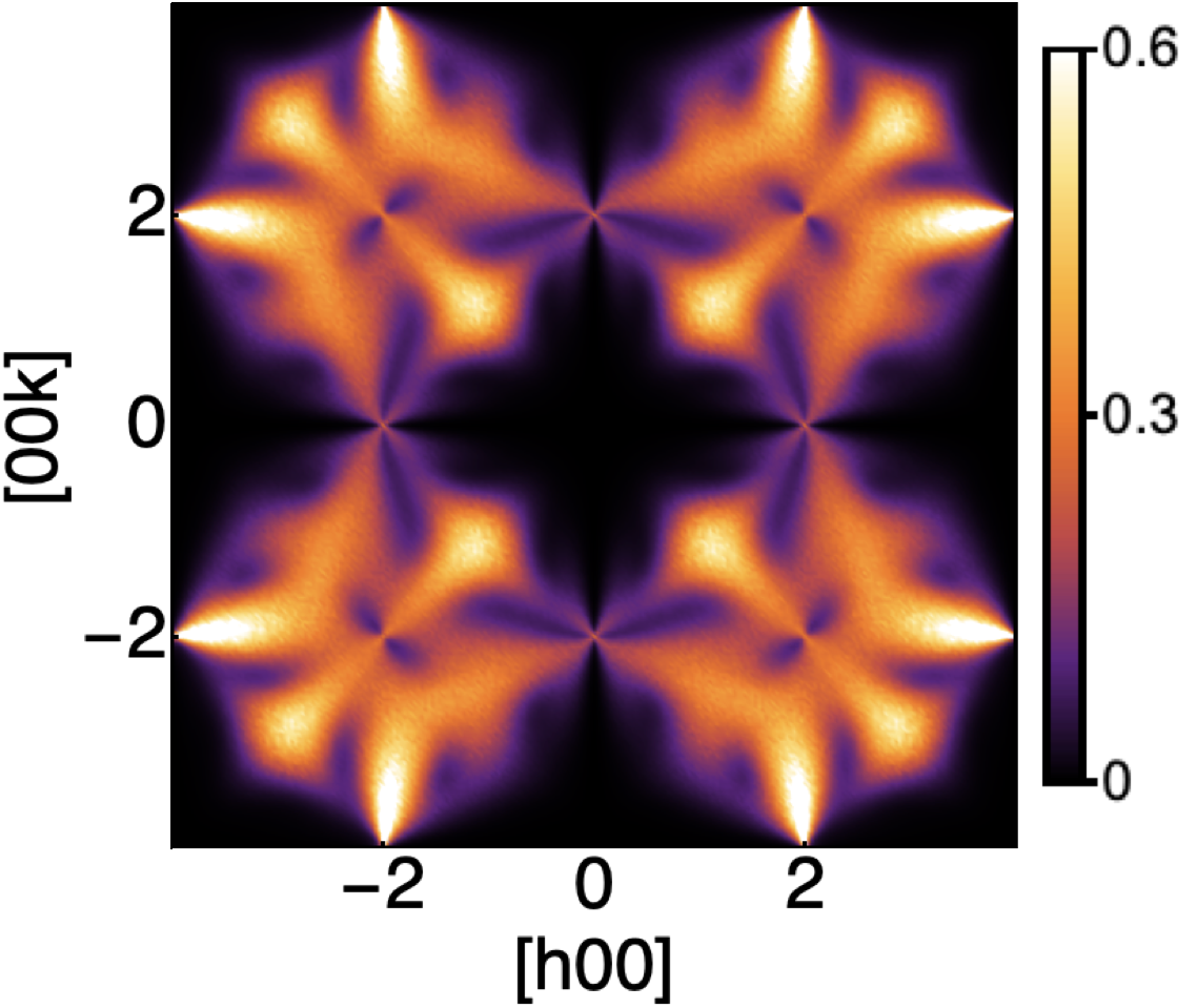
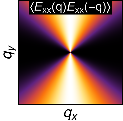
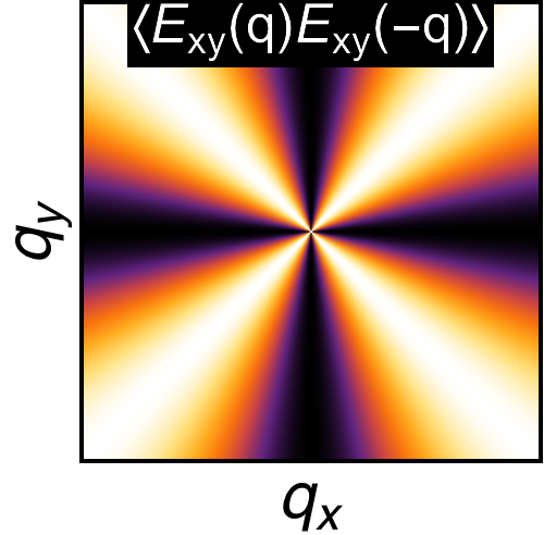
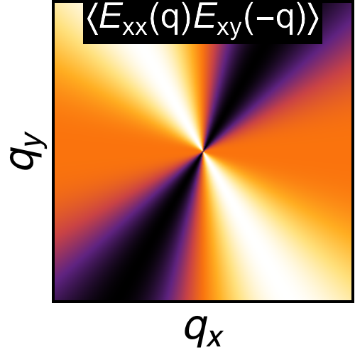
The three–dimensional structure of the correlation $\langle E_{\sf xy}({\bf q})E_{\sf xy}({\bf-q})\rangle$ is illustrated in Fig. 1. In the $[0kl]$ plane, correlations exhibit a conventional 2–fold pinch point, comparable to that found in spin ice [Fig. 1b]. However in the perpendicular $[hk0]$ plane, we observe a 4–fold pinch point (4FPP) [Fig. S1], which unambiguously distinguishes R2–U1 electrodynamics from lower–rank theories Prem et al. (2018).

Comparison with simulation. We can use the existence of this 4FPP as a test for the R2–U1 spin liquid in simulation. We have carried out classical Monte Carlo (MC) simulations of Eq. (6), for the parameter–set

$$J_{A}=J_{B}=1\;,\;D_{A}=-0.01\;,\;D_{B}=0\;.$$ (18)

where the constraints Eq. (2) and Eq. (4) are expected to hold. The resulting correlations of $E_{ij}$, at a temperature $T=2.5\times 10^{-3}\ J_{A}$, are shown in Fig. 1d. For ${\bf q}\to 0$, these are identical to the predictions of Eq. (17), confirming that the model realizes an R2–U1 spin liquid.

Phase diagram. The results of simulations for a range of values of $D_{A}$ are collected in Fig. 2. At finite temperature, a finite value of $D_{A}<0$ is required to achieve a crossover from the $U(1)\times U(1)\times U(1)$ spin liquid of the pyrochlore HAF, with 2–fold pinch points, into an R2–U1 spin liquid, with 4FPP. An analytic theory of this crossover, which is controlled by the dimensionless parameter $\eta\sim|D_{A}|/k_{B}T$, is provided in Section VI of the Supplemental Material. Meanwhile, at low temperatures, sufficiently negative values of $D_{A}$ drive a first–order phase transition into an ordered state which involves the characteristic wavevector ${\bf q}={\bf W}$ (i.e. corners of the Brillouin zone) . In contrast, a finite value of $D_{A}>0$ leads to a continuous phase transition into a state with ${\bf q}=0$, all–out (AIAO) order.

Predictions for neutron scattering. Neutron scattering experiments do not measure correlations of $E_{ij}$ directly, but rather the spin structure factor $S^{\alpha\beta}({\bf q})=\langle S^{\alpha}({\bf q})S^{\beta}(-{\bf q})\rangle$. On general grounds Prem et al. (2018), $S^{\alpha\beta}({\bf q})$ is expected to bear witness to the singularity in Eq. (17). But exactly how 4FPPs would manifest themselves in experiment remains an open question. In Fig. 3 we present simulation results for $S^{\alpha\beta}({\bf q})$ for parameters equivalent to Fig. 3a. We find that the 4FPP is not visible in the structure factor measured by unpolarised neutron scattering [see Supplemental Material]. However the 4FPP can be resolved using polarised neutrons. In this case, it manifests itself in the spin–flip (SF) channel for neutrons polarised perpendicular to the scattering plane Fennell et al. (2009), [Fig. S1].

Application to materials. Breathing–pyrochlore magnets were first studied as a tractable limit of the pyrochlore HAF Harris et al. (1991); Canals and Lacroix (1998, 2000); Tsunetsugu (2001), but have since been realised in materials based on both transition–metal Okamoto et al. (2013); Tanaka et al. (2014); Nilsen et al. (2015); Wawrzyńczak et al. (2017); Okamoto et al. (2018) and rare–earth ions Kimura et al. (2014); Haku et al. (2016). Interesting parallels are also found in lacunar spinels Widmann et al. (2016); Jeong et al. (2017). To date, most theoretical work has concentrated on $SU(2)$–invariant models Harris et al. (1991); Canals and Lacroix (1998, 2000); Tsunetsugu (2001); Benton and Shannon (2015); Li et al. (2016); Essafi et al. (2017). However, in the presence of spin–orbit coupling, the symmetry of the lattice permits anisotropic exchange Rau et al. (2016); Haku et al. (2016); Savary et al. (2016); Rau and Gingras (2018). And, with respect to higher–rank gauge theories, a promising line of enquiry are Yb–based materials, where the required form of interactions appear to predominate.

One concrete example is Ba₃Yb₂Zn₅O₁₁ Kimura et al. (2014); Rau et al. (2016); Haku et al. (2016); Rau and Gingras (2018), where A–tetrahedra are estimated to have the coupling parameters $J_{A}\approx 0.57\ \text{meV}$, $D_{A}\approx-0.16\ \text{meV}$, with other interactions negligible. This is exactly the form of interactions needed for an R2–U1 spin liquid, a feature which is expected to be robust Rau and Gingras (2018), since it holds for a wide range of Slater–Koster overlap ratios Slater and Koster (1954). Meanwhile, exchange interactions on the larger B–tetrahedra of Ba₃Yb₂Zn₅O₁₁, while less well understood, appear to be orders of magnitude smaller Rau et al. (2016); Haku et al. (2016). Thus, while it seems plausible that Ba₃Yb₂Zn₅O₁₁ could realise a R2–U1 spin liquid, this may occur at temperatures too low to measure.

(a) $S_{\sf SF}({\bf q})$, $D_{B}=0$

(b) $S_{\sf SF}({\bf q})$, $D_{B}\ll D_{A}$

Figure 3: Spin structure factor found in MC simulation of the BP model, Eq. (6), showing 4–fold pinch points (4FPPs) characteristic of a R2–U1 spin liquid. (a) Correlations in the $[h0k]$ plane, in the spin–flip (SF) channel measured using polarised neutrons. 4FPP are visible at $[0,0,2]$ and points related by symmetry. Results are for parameters Eq. (18), $T=2.5\times 10^{-3}J_{A}$. (b) Equivalent results for parameters motivated by Ba₃Yb₂Zn₅O₁₁, Eq. (19), $T=252\ \text{mK}$.

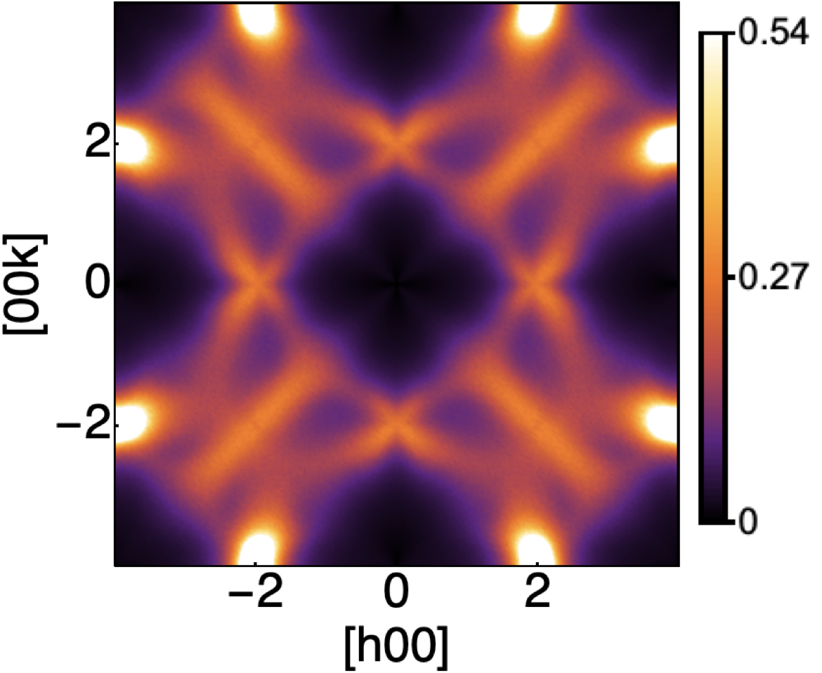
The encouraging example of Ba₃Yb₂Zn₅O₁₁ motivates us to consider the possibility of a magnet with similar structure, but smaller B–tetrahedra, such that the interactions on the B–sublattice become non–negligible. For concreteness, we consider a parameter set:

$$J_{A}=0.57\ \text{meV},\;J_{B}=0.028\ \text{meV}\;,$$

$$D_{A}=-0.16\ \text{meV},\;D_{B}=-0.007\ \text{meV}\;,$$ (19)

where we assume that the interactions on the B–sublattice are of the same form as on the A–sublattice, but substantially weaker, $J_{A}/J_{B}=D_{A}/D_{B}\approx 20$. To demonstrate that the R2–U1 physics persists in the presence of finite $D_{B}$ we have used MC simulation to calculate the spin structure factor. Once again, the 4FPP associated with the R2–U1 spin liquid remains clearly visible for a range of temperatures [Fig. 3b]. The same will hold for a more general choice of interactions, as long as the anisotropic part of the exchange on the B–sublattice is sufficiently weak; for $D_{B}\sim D_{A}$, fluctuations are restricted to the local easy plane, and the R2–U1 physics will be lost.

Quantum effects. The theory of an R2–U1 spin liquid presented above is classical, so it is important to ask what might change once quantum effects are taken into account. A useful point of comparison is quantum spin ice (QSI), where quantum fluctuations leads to tunnelling between different spin configurations satisfying the “ice rules” constraint Eq. (1). This tunnelling, which occurs on loops of spins, introduces a fluctuating magnetic field ${\bf B}$, and the result, at $T=0$, is a QSL described by a the deconfined phase of a $U(1)$ quantum lattice gauge theory Hermele et al. (2004); Banerjee et al. (2008); Benton et al. (2012); Savary and Balents (2012); Shannon et al. (2012); Hao et al. (2014); Gingras and McClarty (2014); Kato and Onoda (2015); Chen (2017); Huang et al. (2018). However it is important to note that the temperature scale associated with this QSL is three orders of magnitude smaller than the range of temperatures over which Eq. (1) holds Huang et al. (2018). Moreover, since the $U(1)$ QSL is gapless, any finite temperature immediately restores classical correlations at long length scales Benton et al. (2012). As a consequence, the spin structure factor $S({\bf q})$ continues to be dominated by pinch–point singularities of the form Eq. (16), down to the lowest temperatures studied Kato and Onoda (2015).

The quantum limit of R2–U1 gauge theories has already been studied as a continuum field theory, and is qualitatively very similar to QSI Pretko (2017a, b); Prem et al. (2018). The lowest lying excitations are gapless emergent photons which modify, but do not eliminate, the singular features observed in scattering Benton et al. (2012); Prem et al. (2018). The microscopic study of quantum effects in Eq. (6) lies outside the scope of this Letter. However we anticipate that coherent gauge fluctuations will be confined to an even lower temperature scale than in QSI, by the fact that the magnetic field $B_{ij}$ is an extended object, involving third–order derivatives of $A_{ij}$ Pretko (2017a, b). For this reason the classical theory developed here should prove sufficient to interpret experiments searching for an R2–U1 in a BP material.

Summary and perspectives. In this Letter, we have used a combination of analytic field theory and classical Monte Carlo simulation to show how a rank–2 $U(1)$ [R2–U1] spin liquid, a state described by a higher–rank generalisation of electrodynamics, can arise in a pyrochlore magnet with breathing anisotropy and Dzyaloshinskii–Moriya interactions, Eq. (6) [cf. Fig. S1]. These results provide a concrete starting point for the experimental search for higher–rank gauge theories, and clarify the type of neutron scattering experiment which would be needed to resolve the 4–fold pinch points (4FPP) of a R2–U1 spin liquid [cf. Fig. 3].

This work opens a number of interesting perspectives. On the experimental side, we identify Yb based breathing–pyrochlore materials as potential candidates for a R2–U1 spin liquid state. On the theoretical side, determining the quantum ground state of Eq. (6), should ultimately prove tractable, since breathing anisotropy provides a natural control parameter for both perturbative Canals and Lacroix (1998, 2000) and variational approaches Benton et al. (2018). And, while the model studied here does not correspond to a fracton stabilizer code upon Higgsing Bulmash and Barkeshli (2018); Ma et al. (2018), the parital–confinement mechanism used to eliminate selected components of the tensorial electric field is very versatile, and easily adapted to generate other versions of R2–U1 theory Yan and Benton (shed).

Acknowledgements. The authors acknowledge helpful conversations with Jeffrey Rau and Daniel Khomskii. This work was supported by the Theory of Quantum Matter Unit, Okinawa Institute of Science and Technology Graduate University (OIST). H.Y. is also supported by Japan Society for the Promotion of Science (JSPS) Research Fellowship for Young Scientists. L. J. acknowledges financial support from the French “Agence Nationale de la Recherche” under Grant No. ANR-18-CE30-0011-01, and hospitality from Gakushuin University under Grants-in-Aid for Scientific Research on innovative areas “Topological Materials Science” (No.JP15H05852) from JSPS. The research was also supported in part by the National Science Foundation under Grant No. NSF PHY-1748958, and the KITP program ”Topological Quantum Matter: From Concepts to Realizations”.

Supplemental Material

I Rank–2 $U(1)$ gauge theory: electrostatics

Here, following Ref. Xu (2006); Pretko (2017a), we derive the relationship between electric, magnetic and gauge fields within the rank–2 $U(1)$ [R2–U1] electrodynamics considered in the main text. This section focuses on the classical electrostatics which is realized in our work. The next section will focus on the quantum dynamics of the theory, which is beyond the scope of this work but nevertheless essential for future developments.

Our starting point is an electric field described by a symmetric, traceless rank–2 tensor,

$$E_{ij}=E_{ji},\quad E_{ii}=0.$$ (S1)

Here we do not distinguish super and subscript since we are dealing with spacial indices.

The low energy sector of the electric field has vanishing vector charge, and is traceless,

$$\partial_{i}E_{ij}=0$$ (S2)

Here we keep all indices as subscripts but still use the Einstein summation rule. The proper rank-2 tensor with the proper Gauss law as a classical spin liquid system is achieved in this work.

II Rank–2 $U(1)$ gauge theory: dynamics

A quantum spin liquid requires quantum dynamics in addition to the emergent Gauss law. Broadly speaking, the dynamics play the role of ${\bf B}^{2}$ term in electrodynamics. They are to tunnel different classical spin liquid states between each other, leading to a long-range entangled quantum ground state and gapless photon excitations. This section explains how to derive such terms and also their implication on mobility of electric charges (fractons).

As in conventional electrodynamics, the conjugate of ${\bf E}$ is the rank-two gauge field $\bf A$, which also has to be symmetric to match the degrees of freedom,

$$A_{ij}=A_{ji}.$$ (S3)

These two conditions determine the form of gauge transformation. Consider a wave-function

$$\ket{\Psi({\bf A})}.$$ (S4)

We take a low energy configuration of $\bf E$ obeying Eq. (S2) and construct a symmetrized operator that is identical to zero to act upon the wave-function

$$-i(\lambda_{j}\partial_{i}E_{ij}+\lambda_{j}\partial_{i}E_{ij})\ket{\Psi({\bf A})}=0.$$ (S5)

By integration by parts and assuming vanishing boundary terms, we have

$$i(\partial_{i}\lambda_{j}+\partial_{i}\lambda_{j})E_{ij}\ket{\Psi({\bf A})}=0.$$ (S6)

Since $E_{ij}$ conjugates with $A_{ij}$, it generates a transformation of $\bf A$. Thus

$$i(\partial_{i}\lambda_{j}+\partial_{i}\lambda_{j})E_{ij}\ket{\Psi({\bf A})}=\ket{\Psi({\bf A}+\bm{\nabla}\otimes\bm{\lambda}+(\bm{\nabla}\otimes\bm{\lambda})^{T})}-\ket{\Psi({\bf A})}=0.$$ (S7)

That is, the low energy sector wave-function is invariant under gauge transformation

$$\begin{split}{\bf A}+\bm{\nabla}\otimes\bm{\lambda}+(\bm{\nabla}\otimes\bm{\lambda})^{T},\quad\text{ i.e., }\quad A_{ij}\rightarrow A_{ij}+\partial_{i}\lambda_{j}+\partial_{i}\lambda_{j}.\end{split}$$ (S8)

Similarly, the traceless condition

$$-i\gamma\delta_{ij}E_{ij}\ket{\Psi({\bf A})}=0.$$ (S9)

leads to another gauge symmetry

$$A_{ij}\rightarrow A_{ij}+\gamma\delta_{ij}.$$ (S10)

Finally, the magnetic field is obtained by finding the simplest gauge-invariant quantity. In this case, it has to have three derivatives acting on the gauge field,

$$\begin{split}B_{ij}=&\frac{1}{2}[\epsilon_{jab}(\partial_{a}\partial_{k}\partial_{i}A_{bk}-\partial_{a}\partial^{2}A_{bi})\\ &+\epsilon_{iab}(\partial_{a}\partial_{k}\partial_{j}A_{bk}-\partial_{a}\partial^{2}A_{bj})].\end{split}$$ (S11)

Finally, the Gauss law, the traceless and symmetric conditions of the electric field can be used to derive:

$$\int dv\vec{\rho}=0$$ (S12)

$$\int dv\vec{x}\times\vec{\rho}=-\int dv\epsilon_{ijk}E_{jk}=0$$ (S13)

$$\int dv\vec{x}\cdot\vec{\rho}=-\int dvE_{ii}=0$$ (S14)

In this case, a vector charge excitation is fully fractonic, i.e., it cannot move in any direction of the system.

Further details of the phenomenology of R2–U1 phases can be found in Refs. Pretko (2017a, b).

III Derivation of Effective Field Theory

We show how a rank–2 tensor electric field, satisfying the constraint required for R2–U1 electrodynamics [Eqs. (1,2)], can be derived from a breathing pyrochlore lattice model [Eq. (6)]. The pattern of this derivation closely follows Refs. Benton et al. (2016); Benton (2014); Yan et al. (2017).

Our starting point is the breathing pyrochlore lattice with a spin on each of its sites, and nearest neighbor interactions between the spins. “Breathing” means the lattice is bi-partitioned into A- and B-tetrahedra [Fig. (1)], and each type of tetrahedron has its own interactions.

The model that hosts a rank-2 spin liquid has breathing Heisenberg antiferromagnetic interactions on both the A- and B-tetrahedra, and negative Dzyaloshinskii-Moriya (DM) interactions on A-tetrahedra only. The Hamiltonian for the model is

$$\mathcal{H}=\sum_{\langle ij\rangle\in\text{A}}\left[J_{A}{\bf S}_{i}\cdot{\bf S}_{j}+D_{A}\hat{\bf d}_{ij}\cdot({\bf S}_{i}\times{\bf S}_{j})\right]+\sum_{\langle ij\rangle\in\text{B}}\left[J_{B}{\bf S}_{i}\cdot{\bf S}_{j}+D_{B}\hat{\bf d}_{ij}\cdot({\bf S}_{i}\times{\bf S}_{j})\right].$$ (S15)

where $\langle ij\rangle\in\text{A(B)}$ denotes nearest neightbour bonds belonging to the A(B)-tetrahedra. The sites $0,\ 1,\ 2,\ 3$ are at positions relative to the center of an A-tetrahedron

$${\bf r}_{0}=\frac{a}{8}(1,1,1),\;{\bf r}_{1}=\frac{a}{8}(1,-1,-1),\;{\bf r}_{2}=\frac{a}{8}(-1,1,-1),\;{\bf r}_{3}=\frac{a}{8}(-1,-1,1),$$ (S16)

where $a$ is the length of the unit cell. Vectors $\hat{\bf d}_{ij}$ are bond dependent, defined in accordance with Ref Kotov et al. (2005); Canals et al. (2008); Rau et al. (2016):

$$\begin{split}&\hat{\bf d}_{01}=\frac{(0,-1,1)}{\sqrt{2}},\;\hat{\bf d}_{02}=\frac{(1,0,-1)}{\sqrt{2}},\;\hat{\bf d}_{03}=\frac{(-1,1,0)}{\sqrt{2}},\\ &\hat{\bf d}_{12}=\frac{(-1,-1,0)}{\sqrt{2}},\;\hat{\bf d}_{13}=\frac{(1,0,1)}{\sqrt{2}},\;\hat{\bf d}_{23}=\frac{(0,-1,-1)}{\sqrt{2}}.\end{split}$$ (S17)

Equivalently, this model can be written in a standard matrix-exchange form for a breathing-pyrochlore lattice model as

$$\mathcal{H}=\sum_{\langle ij\rangle\in\text{A}}S_{i}^{\alpha}\mathcal{J}_{\text{A,ij}}^{\alpha\beta}S_{j}^{\beta}+\sum_{\langle ij\rangle\in\text{B}}S_{i}^{\alpha}\mathcal{J}_{\text{B}}^{\alpha\beta}S_{j}^{\beta}$$ (S18)

where $\mathcal{J}_{\text{A,ij}}$ is a three-by-three matrix that couples spins on sub-lattice sites $i,j$ whose bond belongs to A-tetrahedra, and $\mathcal{J}_{\text{B}}$ is the coupling matrix for B-tetrahedra. In the case of $D_{B}=0$ that we are interested in, $\mathcal{J}_{\text{B}}$ is identical for any pair of $i,j$,

$$\mathcal{J}_{\text{B}}=\begin{bmatrix}J_{B}&0&0\\ 0&J_{B}&0\\ 0&0&J_{B}\end{bmatrix}.$$ (S19)

Matrices $\mathcal{J}_{\text{A,ij}}$ are bond dependent and related to each other by the lattice symmetry. Their values are

$$\begin{split}&\mathcal{J}_{\text{A,01}}=\begin{bmatrix}J_{A}&D_{A}/\sqrt{2}&D_{A}/\sqrt{2}\\ -D_{A}/\sqrt{2}&J_{A}&0\\ -D_{A}/\sqrt{2}&0&J_{A}\end{bmatrix},\;\mathcal{J}_{\text{A,02}}=\begin{bmatrix}J_{A}&-D_{A}/\sqrt{2}&0\\ D_{A}/\sqrt{2}&J_{A}&D_{A}/\sqrt{2}\\ 0&-D_{A}/\sqrt{2}&J_{A}\end{bmatrix},\;\\ &\mathcal{J}_{\text{A,03}}=\begin{bmatrix}J_{A}&0&-D_{A}/\sqrt{2}\\ 0&J_{A}&-D_{A}/\sqrt{2}\\ D_{A}/\sqrt{2}&D_{A}/\sqrt{2}&J_{A}\end{bmatrix},\;\mathcal{J}_{\text{A,12}}=\begin{bmatrix}J_{A}&0&D_{A}/\sqrt{2}\\ 0&J_{A}&-D_{A}/\sqrt{2}\\ -D_{A}/\sqrt{2}&D_{A}/\sqrt{2}&J_{A}\end{bmatrix},\;\\ &\mathcal{J}_{\text{A,13}}=\begin{bmatrix}J_{A}&D_{A}/\sqrt{2}&0\\ -D_{A}/\sqrt{2}&J_{A}&D_{A}/\sqrt{2}\\ 0&-D_{A}/\sqrt{2}&J_{A}\end{bmatrix},\;\mathcal{J}_{\text{A,23}}=\begin{bmatrix}J_{A}&-D_{A}/\sqrt{2}&D_{A}/\sqrt{2}\\ D_{A}/\sqrt{2}&J_{A}&0\\ -D_{A}/\sqrt{2}&0&J_{A}\end{bmatrix}.\end{split}$$ (S20)

order	definition in terms	associated
parameter	of spin components	ordered phases
$m_{\sf A_{2}}$	$\frac{1}{2\sqrt{3}}\left(S_{0}^{x}+S_{0}^{y}+S_{0}^{z}+S_{1}^{x}-S_{1}^{y}-S_{1}^{z}-S_{2}^{x}+S_{2}^{y}-S_{2}^{z}-S_{3}^{x}-S_{3}^{y}+S_{3}^{z}\right)$	“all in-all out”
${\bf m}_{\sf E}$	$\begin{pmatrix}\frac{1}{2\sqrt{6}}\left(-2S_{0}^{x}+S_{0}^{y}+S_{0}^{z}-2S_{1}^{x}-S_{1}^{y}-S_{1}^{z}+2S_{2}^{x}+S_{2}^{y}-S_{2}^{z}+2S_{3}^{x}-S_{3}^{y}+S_{3}^{z}\right)\\ \frac{1}{2\sqrt{2}}\left(-S_{0}^{y}+S_{0}^{z}+S_{1}^{y}-S_{1}^{z}-S_{2}^{y}-S_{2}^{z}+S_{3}^{y}+S_{3}^{z}\right)\end{pmatrix}$	$\begin{matrix}\Gamma_{5},\textrm{including}\\ \Psi_{2}\textrm{ and }\Psi_{3}\end{matrix}$
${\bf m}_{\sf T_{1+}}$	$\begin{pmatrix}\frac{1}{2}(S_{0}^{x}+S_{1}^{x}+S_{2}^{x}+S_{3}^{x})\\ \frac{1}{2}(S_{0}^{y}+S_{1}^{y}+S_{2}^{y}+S_{3}^{y})\\ \frac{1}{2}(S_{0}^{z}+S_{1}^{z}+S_{2}^{z}+S_{3}^{z})\end{pmatrix}$	collinear FM
${\bf m}_{\sf T_{1,-}}$	$\begin{pmatrix}\frac{-1}{2\sqrt{2}}(S_{0}^{y}+S_{0}^{z}-S_{1}^{y}-S_{1}^{z}-S_{2}^{y}+S_{2}^{z}+S_{3}^{y}-S_{3}^{z})\\ \frac{-1}{2\sqrt{2}}(S_{0}^{x}+S_{0}^{z}-S_{1}^{x}+S_{1}^{z}-S_{2}^{x}-S_{2}^{z}+S_{3}^{x}-S_{3}^{z})\\ \frac{-1}{2\sqrt{2}}(S_{0}^{x}+S_{0}^{y}-S_{1}^{x}+S_{1}^{y}+S_{2}^{x}-S_{2}^{y}-S_{3}^{x}-S_{3}^{y})\end{pmatrix}$	non-collinear FM
${\bf m}_{\sf T_{2}}$	$\begin{pmatrix}\frac{1}{2\sqrt{2}}\left(-S_{0}^{y}+S_{0}^{z}+S_{1}^{y}-S_{1}^{z}+S_{2}^{y}+S_{2}^{z}-S_{3}^{y}-S_{3}^{z}\right)\\ \frac{1}{2\sqrt{2}}\left(S_{0}^{x}-S_{0}^{z}-S_{1}^{x}-S^{z}_{1}-S_{2}^{x}+S_{2}^{z}+S_{3}^{x}+S_{3}^{z}\right)\\ \frac{1}{2\sqrt{2}}\left(-S_{0}^{x}+S_{0}^{y}+S_{1}^{x}+S_{1}^{y}-S_{2}^{x}-S_{2}^{y}+S_{3}^{x}-S_{3}^{y}\right)\end{pmatrix}$	Palmer–Chalker ($\Psi_{4}$)

Table 1: Order parameters ${\bf m}_{\mathsf{X}}$, describing how the point-group symmetry of a single tetrahedron within the pyrochlore lattice is broken by magnetic order. Order parameters transform according to irreducible representations of the point-group ${\sf T}_{d}$, and are expressed in terms of linear combinations of spin-components ${\bf S}_{i}=(S^{x}_{i},S^{y}_{i},S^{z}_{i})$, in the global frame of the crystal axes — cf. $\mathcal{H}$ [Eq. (S15))]. Labelling of spins within the tetrahedron follows the convention of Ross et al. Ross et al. (2011). The notation $\Psi_{i}$ for ordered phases is taken from Ref. Poole et al. (2007).

The spin degrees of freedom on each tetrahedron can be rewritten in terms of fields forming the irreducible representations of the lattice symmetry,

$${m}_{\mathsf{A_{2}}},\quad\mathbf{m}_{\mathsf{E}},\quad\mathbf{m}_{\mathsf{T_{2}}},\quad\mathbf{m}_{\mathsf{T_{1+}}},\quad\mathbf{m}_{\mathsf{T_{1-}}},$$ (S21)

whose definition can be found in Table 1. They are linear combinations of the spin degrees of freedom, allowing for a fully quadratic Hamiltonian:

$$\mathcal{H}=\frac{1}{2}\sum_{\mathsf{X}}a_{\mathsf{X},\text{A}}m^{2}_{\mathsf{X},\text{A}}+\frac{1}{2}\sum_{\mathsf{X}}a_{\mathsf{X},\text{B}}m^{2}_{\mathsf{X},\text{B}},$$ (S22)

where $\mathsf{X}$ runs over irreps of the group $T_{d}$, i.e. $\{\mathsf{A_{2}},\mathsf{E},\mathsf{T_{2}},\mathsf{T_{1+}},\mathsf{T_{1-}}\}$ as listed in Eq. (S21), and the subscript A,B denotes on which type of tetrahedra they are defined. The coefficients $a_{\mathsf{X}}$ are listed in Table. 2.

coefficient of $|{\bf m}_{\mathsf{X}}|^{2}$ in Eq.(S22)	definition in terms of $J$ and $D$
$a_{\mathsf{A_{2}}}$	$-J-4D/\sqrt{2}$
$a_{\mathsf{E}}$	$-J+2D/\sqrt{2}$
$a_{\mathsf{T_{2}}}$	$-J-2D/\sqrt{2}$
$a_{\mathsf{T_{+}}}$	$3J$
$a_{\mathsf{T_{-}}}$	$-J+2D/\sqrt{2}$

Table 2: Coefficients $a_{\mathsf{X}}$ of the irrep invariants $|{\bf m}_{\mathsf{X}}|^{2}$ appearing in $\mathcal{H}$ [Eq.(S22)]. Coefficients are expressed as a function of $J$ and $D$. Here the subscripts for the A- and B-tetrahedra are suppressed.

For the couplings in Eq. (S15), we have on A-tetrahedra

$$a_{\mathsf{A_{2}},\text{A}} = -J_{A}-4D_{A}/\sqrt{2}\;,$$ (S23)

$$a_{\mathsf{T_{2}},\text{A}} = -J_{A}-2D_{A}/\sqrt{2}\;,$$ (S24)

$$a_{\mathsf{T_{1+}},\text{A}} = 3J_{A}\;,$$ (S25)

$$a_{\mathsf{T_{1-}},\text{A}}=a_{\mathsf{E},\text{A}} = -J_{A}+2D_{A}/\sqrt{2},$$ (S26)

and on B-tetrahedra

$$a_{\mathsf{A_{2}},\text{B}}=a_{\mathsf{E},\text{B}}=a_{\mathsf{T_{2}},\text{B}}=a_{\mathsf{T_{1-}},\text{B}} = -J_{B},$$ (S27)

$$a_{\mathsf{T_{1+}},\text{B}} = 3J_{B}.$$ (S28)

For $J_{A},J_{B}>0$ and $D_{A}<0$, these parameters are in order

$$\text{on A-tetrahedra:}\qquad a_{\mathsf{E},\text{A}}=a_{\mathsf{T_{1-}},\text{A}}<a_{\mathsf{A_{2}},\text{A}},\ a_{\mathsf{T_{2}},\text{A}},\ a_{\mathsf{T_{1+}},\text{A}},$$ (S29)

$$\text{on B-tetrahedra:}\qquad a_{\mathsf{A_{2}},\text{B}}=a_{\mathsf{E},\text{B}}=a_{\mathsf{T_{2}},\text{B}}=a_{\mathsf{T_{1-}},\text{B}}<a_{\mathsf{T_{1+}},\text{B}},$$ (S30)

which plays the central role of dictating the low energy physics.

The irreducible representation fields are subject to constraints arising from fixed spin length

$$\sum_{\mathsf{X}}m^{2}_{\mathsf{X}}=1$$ (S31)

for both A- and B-tetrahedra. As a consequence, the low energy sector allows the $m^{2}_{\mathsf{X}}$ corresponding to the smallest $a_{\mathsf{X}}$ to fluctuate, while all other fields have to vanish. This principle applied to our model leads to

• On A-tetrahedra, the fields $\mathbf{m}_{\mathsf{E}}$ and $\mathbf{m}_{\mathsf{T_{1-}}}$ can fluctuate;

• On A-tetrahedra, the fields ${\bf m}_{\mathsf{T_{1+}}}={\bf m}_{\mathsf{T_{2}}}=\mathbf{0},\ {m}_{\mathsf{A_{2}}}=0$;

• On B-tetrahedra, the fields ${m}_{\mathsf{A_{2}}},\;\mathbf{m}_{\mathsf{E}},\;\mathbf{m}_{\mathsf{T_{2}}},\;\mathbf{m}_{\mathsf{T_{1-}}}$ can fluctuate;

• On B-tetrahedra,

  $${\bf m}_{\mathsf{T_{1+}}}=0$$ (S32)

Since every spin is shared by an A- and a B-tetrahedron, the fluctuating fields $\mathbf{m}_{\mathsf{E}}$ and $\mathbf{m}_{\mathsf{T_{1-}}}$ on A-tetrahedra must obey additional constraints to respect the the low-energy sector condition on B-tetrahedron imposed by Eq. (S32). Assuming that the fields are varying slowly in space such that the continuous limit can be taken, the constraint Eq. (S32) can be expressed in terms of fields living on A-tetrahedron as

$$\frac{2}{\sqrt{3}}\begin{bmatrix}\partial_{x}m_{\mathsf{E}}^{1}\\ -\frac{1}{2}\partial_{y}m_{\mathsf{E}}^{1}-\frac{\sqrt{3}}{2}\partial_{y}m_{\mathsf{E}}^{2}\\ -\frac{1}{2}\partial_{y}m_{\mathsf{E}}^{1}+\frac{\sqrt{3}}{2}\partial_{y}m_{\mathsf{E}}^{2}\end{bmatrix}-\begin{bmatrix}\partial_{y}m_{\mathsf{T_{1-}}}^{z}+\partial_{z}m_{\mathsf{T_{1-}}}^{y}\\ \partial_{z}m_{\mathsf{T_{1-}}}^{x}+\partial_{x}m_{\mathsf{T_{1-}}}^{z}\\ \partial_{x}m_{\mathsf{T_{1-}}}^{y}+\partial_{y}m_{\mathsf{T_{1-}}}^{x}\end{bmatrix}=0.$$ (S33)

From this constraint we can build the symmetric, traceless, rank-two magnetic field $E_{ij}$ as

$$E_{ij}=\begin{bmatrix}\frac{2}{\sqrt{3}}m_{\mathsf{E}}^{1}&m_{\mathsf{T_{1-}}}^{z}&m_{\mathsf{T_{1-}}}^{y}\\ m_{\mathsf{T_{1-}}}^{z}&-\frac{1}{\sqrt{3}}m_{\mathsf{E}}^{1}-m_{\mathsf{E}}^{2}&m_{\mathsf{T_{1-}}}^{x}\\ m_{\mathsf{T_{1-}}}^{y}&m_{\mathsf{T_{1-}}}^{x}&-\frac{1}{\sqrt{3}}m_{\mathsf{E}}^{1}+m_{\mathsf{E}}^{2}\end{bmatrix}\;,$$ (S34)

such that Eq. (S33) becomes

$$\partial_{i}E_{ij}=0\;,$$ (S35)

with symmetric and traceless conditions

$$E_{ji}=E_{ji},\qquad\operatorname{Tr}{\bf E}=0$$ (S36)

by the definition of $E_{ij}$. Hence a rank-2, traceless, vector charged magnetic field emerges at the low-energy sector from the microscopic model of Eq. (S15).

Equation (S36) constrains the form of correlations functions of $\langle E_{ij}({\bf q})E_{kl}(-{\bf q})\rangle$, in the same spirit as how the two-in-two-out condition constrains the spin-spin correlation of spin ice. It is, however, in a more complicated form. The explicit results for the traceful scalar-charged and vector-charged versions of R2–U1 are discussed in detail in Ref. Prem et al. (2018). The vector-charge field correlation is

$$\begin{split}\langle E_{ij}({\bf q})E_{kl}(-{\bf q})\rangle\propto&\frac{1}{2}(\delta_{ik}\delta_{jl}+\delta_{il}\delta_{jk})+\frac{q_{i}q_{j}q_{k}q_{l}}{q^{4}}\\ &-\frac{1}{2}\left(\delta_{ik}\frac{q_{i}q_{l}}{q^{2}}+\delta_{jk}\frac{q_{i}q_{l}}{q^{2}}+\delta_{il}\frac{q_{j}q_{k}}{q^{2}}+\delta_{jl}\frac{q_{i}q_{k}}{q^{2}}\right)\end{split}$$ (S37)

In close analogy, we derive the correlation function of our traceless vector-charged model by deducting the trace,

$$\begin{split}\langle E_{ij}({\bf q})E_{kl}(-{\bf q})\rangle\propto&\frac{1}{2}(\delta_{ik}\delta_{jl}+\delta_{il}\delta_{jk})+\frac{q_{i}q_{j}q_{k}q_{l}}{q^{4}}\\ &-\frac{1}{2}\left(\delta_{ik}\frac{q_{i}q_{l}}{q^{2}}+\delta_{jk}\frac{q_{i}q_{l}}{q^{2}}+\delta_{il}\frac{q_{j}q_{k}}{q^{2}}+\delta_{jl}\frac{q_{i}q_{k}}{q^{2}}\right)\\ &-\frac{1}{2}\left(\delta_{ij}-\frac{q_{i}q_{j}}{q^{2}}\right)\left(\delta_{kl}-\frac{q_{k}q_{l}}{q^{2}}\right),\end{split}$$ (S38)

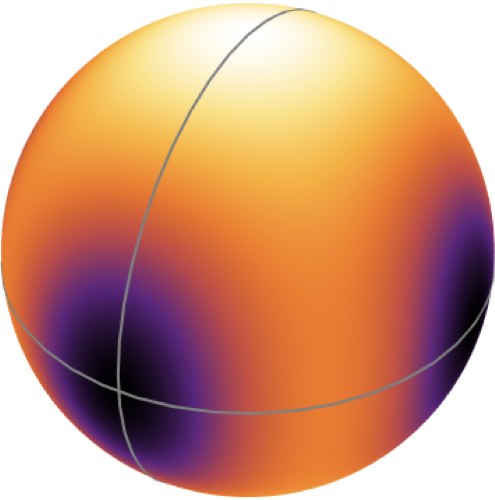
which encodes a singularity at ${\bf q}\rightarrow 0$. Different choices of the components $E_{ij}$ and $E_{kl}$ show different patterns. A few representative ones can be found in Figs. S1,S2a.

(a)

(b)

(c)

Figure S1: Structure of the 4–fold pinch point (4FPP) associated with rank–2 $U(1)$ [R2–U1] gauge theory. (a) Prediction of R2–U1 theory for the correlation function $\langle E_{\sf xy}({\bf q})E_{\sf xy}({\bf-q})\rangle$, on a surface of fixed $|{\bf q}|$ near to a Brillouin zone center. (b) Exploded view, showing a 2–fold pinch point in the [0kl] plane. (c) Perpendicular cut, showing a 4FPP in the [hk0] plane.

(a)

(b)

(c)

(d)

(e)

Figure S2: Different components of correlation function $\langle E_{ij}({\bf q})E_{kl}(-{\bf q})\rangle$ in $q_{x}-q_{y}$ plane, calculated from Eq. (S38).

     

Fig. S2b,S2c have the four-fold pinch-point (4FPP) singularity, which differentiates the rank-2 gauge theories uniquely from the conventional $U(1)$ gauge theory. It is the key signature to be looked for in experiments.

IV Alternative forms of R2–U1 spin liquid

In the main text we have shown how a classical spin liquid described by a symmetric, traceless R2–U1 gauge theory, descends from the $U(1)\times U(1)\times U(1)$ spin liquid found in the classical Heisenberg Antiferromagnet (HAF) on a pyrochlore lattice. The approach taken is very versatile, and by tuning the Hamiltonian, one can also obtain other forms of R2–U1 spin liquid.

Notice that the diagonal and off-diagonal components of ${\bf E}^{\sf HAF}_{\sf sym.}$ come from different irreps ${\bf m}_{\mathsf{E}}$ and ${\bf m}_{\mathsf{T_{1-}}}$. In the most general Hamiltonian (Eq.S22), these two irreps have their individually tunable coefficients $a_{\mathsf{E}}$ and $a_{\mathsf{T_{1-}}}$. So the symmetric part of ${\bf E}^{\sf HAF}$ can be decomposed into three components

$${\bf E}^{\sf HAF}_{\sf trace}+{\bf E}^{\sf HAF}_{\sf sym-diagonal}+{\bf E}^{\sf HAF}_{\sf symm-off-diagonal},$$ (S39)

and each component can be individually tuned to be active or suppressed by choosing the proper Hamiltonian. The vector-charged Gauss law is unaffected. This allows us to build a variety of rank-2 U(1) gauge theories, including a “hollow” version with vanishing diagonal terms Ma et al. (2018) .

V Predictions for Neutron Scattering

The 4FPP is a unique pattern that differentiates the R2–U1 from vector $U(1)$ gauge theory, which only has the conventional two-fold pinch points. The 4FPPs are most unambiguously presented in the correlation function of the irrep fields as discussed in the main text. These correlation functions are, however, not directly accessible in experiment.

In magnetism, neutron scattering is widely used to measure the spin-spin correlation of the form

$$S({\bf q})=\sum_{\alpha,\beta,i,j}\left(\delta_{\alpha\beta}-\frac{q^{\alpha}q^{\beta}}{q^{2}}\right)\langle S_{i}^{\alpha}({\bf q})S_{j}^{\beta}(-{\bf q})\rangle$$ (S40)

where $\alpha,\beta=x,y,z$ are spin-component indices and $i,j=0,1,2,3$ are sub-lattice site indices.

Furthermore, with neutrons polarized in direction of unit vector $\hat{\bf v}$ perpendicular to the scattering plane, one can measure the spin-flip (SF) channel neutron scattering defined by

$$S({\bf q})_{\text{SF}}=\sum_{\alpha,\beta,i,j}(v_{\perp}^{\alpha}v_{\perp}^{\beta})\langle S_{i}^{\alpha}({\bf q})S_{j}^{\beta}(-{\bf q})\rangle,$$ (S41)

where

$$\hat{\bf v}_{\perp}=\frac{\hat{\bf v}\times{\bf q}}{|\hat{\bf v}\times{\bf q}|}.$$ (S42)

One can also measure the non-spin-flip (NSF) channel defined by

$$S({\bf q})_{\text{NSF}}=\sum_{\alpha,\beta,i,j}(v^{\alpha}v^{\beta})\langle S_{i}^{\alpha}({\bf q})S_{j}^{\beta}(-{\bf q})\rangle$$ (S43)

Here we show the spin structure factor of the $[h0k]$ and $[hhk]$ plane, with zoomed-in view of the 4FPPs.

Figure S3: 4-Fold Pinch Points (4FPPs) in spin structure factor in the $[h0k]$ and $[hhk]$ plane of momentum space of the model [Eq. (6)] from MC simulations. The exchange parameters are from the idealized theoretical case $J_{A}=J_{B}=1.0,\ D_{A}=-0.01,\ D_{B}=0.0$, at $T=2.5\times 10^{-3}\ J_{A}$. (a) Total structure factor in $[h0k]$ plane. (b) Non-spin-flip (NSF) channel in $[h0k]$ plane. (c) Spin-flip (SF) channel in $[h0k]$ plane. (d) Enlarged 4FPP in $[h0k]$ plane. (a) Total structure factor in $[hhk]$ plane. (b) Non-spin-flip (NSF) channel in $[hhk]$ plane. (c) Spin-flip (SF) channel in $[hhk]$ plane. (d) Enlarged 4FPP in $[hhk]$ plane. The 4FPPs can be clearly observed in the SF channel, centered on [0, 0, 2] (and points related by symmetry), but weaker than in the $[h0k]$ plane.

Figure S4: 4-Fold Pinch Points (4FPPs) in spin structure factors in the $[h0k]$ and $[hhk]$ planes of momentum space of the model [Eq. (6)] from MC simulations. The exchange parameters are from the experimental case Eq. (19) at $T=252\ \text{mK}$. (a) Total structure factor in $[h0k]$ plane. (b) Non-spin-flip (NSF) channel in $[h0k]$ plane. (c) Spin-flip (SF) channel in $[h0k]$ plane. (d) Enlarged 4FPP in $[h0k]$ plane. (a) Total structure factor in $[hhk]$ plane. (b) Non-spin-flip (NSF) channel in $[hhk]$ plane. (c) Spin-flip (SF) channel in $[hhk]$ plane. (d) Enlarged 4FPP in $[hhk]$ plane. The 4FPPs can be observed in the SF channel, centered on [0, 0, 2] (and points related by symmetry), but weaker than in the $[h0k]$ plane.

VI Temperature evolution of 4–fold pinch point into a conventional 2–fold pinch point

The cross–over from the HAF phase to the R2–U1 phase, with decreasing temperature, is manifested in the structure factor as a cross–over between a conventional, 2–fold, pinch point and the 4–fold pinch point (4FPP) characteristic of an R2–U1 gauge theory Prem et al. (2018). To provide further quantitative details of this cross–over, here we present an analysis of correlations based on a coarse–grained field theory.

As shown above, the $U(1)\times U(1)\times U(1)$ spin liquid of the Heisenberg model can be described in terms of a non-symmetric matrix ${\bf E}$, with a Gauss’ law applied to each column. The traceless R2-U(1) spin liquid is described in the same way, but with the constraint that ${\bf E}$ be symmetric and traceless.

The following effective theory captures both cases:

$$\mathcal{Z}=\int\prod_{\mu,\nu}dE_{\mu\nu}\exp(-\beta H_{eff}[E_{\mu\nu}])$$ (S44)

$$\beta H_{eff}=\frac{\lambda}{2}\int d^{3}{\bf r}\bigg{(}\sum_{\mu\nu}E_{\mu\nu}^{2}+\delta\sum_{\nu}\bigg{[}\sum_{\mu}\partial_{\mu}E_{\mu\nu}\bigg{]}^{2}+\eta\bigg{[}\frac{1}{3}{\rm Tr}[{\bf E}]^{2}+\frac{1}{2}(E_{xy}-E_{yx})^{2}+\frac{1}{2}(E_{xz}-E_{zx})^{2}+\frac{1}{2}(E_{yz}-E_{zy})^{2}\bigg{]}\bigg{)}$$

(S45)

where the integral in Eq. (S44) is taken independently over all components of the matrix ${\bf E}$ and $\beta=1/T$ is the inverse temperature.

The limit $\delta\to\infty,\eta\to 0$, captures the Heisenberg model spin liquid, with Gauss’ law enforced on every column of ${\bf E}$ and no correlations between columns. The limit $\delta\to\infty,\eta\to\infty$ captures the R2-U(1) spin liquid, with ${\bf E}$ forced to be symmetric and traceless and still obeying Gauss’ law for each column.

In terms of the parameters of the microscopic model:

$$\delta\sim\beta J,\quad\eta\sim\beta|D_{A}|.$$ (S46)

since $\delta$ is the coefficient enforcing the Gauss’ law (which is generated by $J$) and $\eta$ is the coefficient enforcing the symmetric and traceless conditions (which are generated by $D_{A}$).

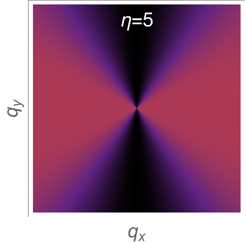
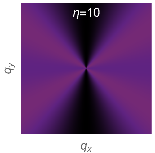
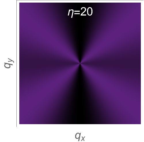
We can study the crossover from the Heisenberg to R2-U(1) spin liquids by first taking $\delta\to\infty$ and observing the behavior as a function of $\eta$. The crossover can be illustrated by calculating the correlation function

$$\langle E^{yx}(\mathbf{q})E^{yx}(-\mathbf{q})\rangle$$

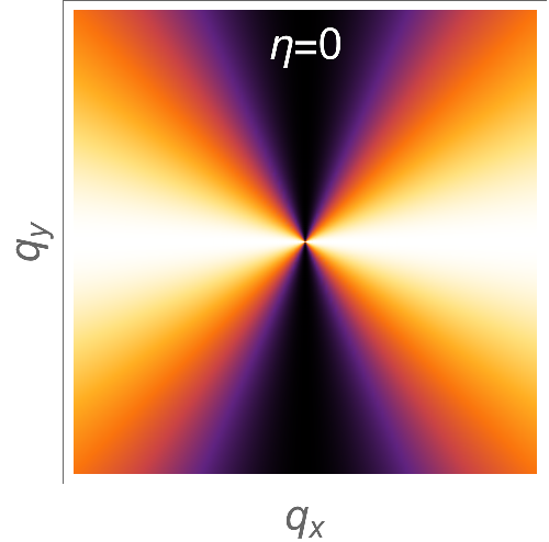
which should have a 2-fold pinch point in the Heisenberg limit and a 4-fold pinch point in the R2-U(1) limit.

Calculating the correlation function from Eqs. (S44)-(S45) and taking the limit $\delta\to\infty$. gives us

$$\langle E^{yx}(\mathbf{q})E^{yx}(-\mathbf{q})\rangle=\frac{f(\mathbf{q},\eta)}{2\lambda q^{4}(1+\eta)(2+\eta)(3+2\eta)}$$ (S47)

$$f(\mathbf{q},\eta)=4q_{x}^{4}(1+\eta)(3+2\eta)+q_{z}^{2}(q_{y}^{2}+qz^{2})(2+\eta)^{2}(3+2\eta)+2q_{x}^{2}q_{y}^{2}(1+\eta)(2+\eta)(3+\eta)+q_{x}^{2}q_{z}^{2}(3+2\eta)(8+8\eta+\eta^{2}).$$

The $\eta\to 0$ limit of Eq. (S47) gives the Heisenberg limit of the correlation function (a 2-fold pinch point)

$$\lim_{\eta\to 0}\langle E^{yx}(\mathbf{q})E^{yx}(-\mathbf{q})\rangle=\frac{1}{\lambda}\left(1-\frac{q_{y}^{2}}{q^{2}}\right).$$ (S49)

Whereas, the $\eta\to\infty$ limit gives the R2-U(1) correlation function (a 4-fold pinch point):

$$\lim_{\eta\to\infty}\langle E^{yx}(\mathbf{q})E^{yx}(-\mathbf{q})\rangle=\frac{1}{2\lambda}\frac{(q^{2}-q_{x}^{2})(q^{2}-q_{y}^{2})}{q^{4}}.$$ (S50)

Since $\eta\sim\beta|D_{A}|$, we can see from Eq. (S47) that for a fixed ${\bf q}$ at any, fixed, finite temperature the evolution as a function of $D_{A}$, will be smooth, although at small temperatures, a small change in $D_{A}$ will give a large change in $\eta$ and hence the correlation function. Only at $T=0$ does the correlation function behave in a singular fashion as a function of $D_{A}$, but this is not surprising, since the Heisenberg limit has a highly degenerate ground state.

The progression of the correlation function as $\eta$ is increased is given in Fig (S5). This progression can either be seen as decreasing the temperature at fixed, small, $|D_{A}|$ or as increasing $|D_{A}|$ at fixed small temperature.

Figure S5: Evolution of the correlation function $\langle E^{yx}(\mathbf{q})E^{yx}(-\mathbf{q})\rangle$ [Eq. (S47)] from a 2-fold pinch point to a 4-fold pinch point as we tune from the Heisenberg to R2-U(1) spin liquids by increasing the parameter $\eta$ [Eq. (S45)]. In terms of our microscopic model, this may be viewed either as decreasing the temperature at fixed, small, $|D_{A}|$ or as increasing $|D_{A}|$ at fixed small temperature.

VII Monte Carlo simulations

Monte Carlo simulations are performed on systems of classical O(3) spins with $16L^{3}$ sites, where $L^{3}$ is the number of cubic unit cells. The spin length is $|S|=1/2$. To decorrelate the system, we use jointly the heatbath method, over-relaxation and parallel tempering. Thermalization is made in two steps: first a slow annealing from high temperature to the temperature of measurement $T$ during $t_{e}$ Monte Carlo steps (MCs) followed by $t_{e}$ MCS at temperature $T$. After thermalization, measurements are done every 10 MCs during $t_{m}=10~{}t_{e}$ MCs. All structure factors have been computed from simulations with $L=30$ and $t_{m}=5\times 10^{5}$ MCs. The phase diagram of Fig. 5 has been computed from simulations with $L=8$ and $t_{m}=10^{7}$ MCs.

References

- Anderson (1972) P. W. Anderson, Science 177, 393 (1972).
- Anderson (1973) P. Anderson, Materials Research Bulletin 8, 153 (1973).
- Balents (2010) L. Balents, Nature (London) 464, 199 (2010).
- Savary and Balents (2017) L. Savary and L. Balents, Reports on Progress in Physics 80, 016502 (2017).
- Zhou et al. (2017) Y. Zhou, K. Kanoda, and T.-K. Ng, Rev. Mod. Phys. 89, 025003 (2017).
- Hermele et al. (2004) M. Hermele, M. P. A. Fisher, and L. Balents, Phys. Rev. B 69, 064404 (2004).
- Banerjee et al. (2008) A. Banerjee, S. V. Isakov, K. Damle, and Y. B. Kim, Phys. Rev. Lett. 100, 047208 (2008).
- Benton et al. (2012) O. Benton, O. Sikora, and N. Shannon, Phys. Rev. B 86, 075154 (2012).
- Savary and Balents (2012) L. Savary and L. Balents, Phys. Rev. Lett. 108, 037202 (2012).
- Shannon et al. (2012) N. Shannon, O. Sikora, F. Pollmann, K. Penc, and P. Fulde, Phys. Rev. Lett. 108, 067204 (2012).
- Hao et al. (2014) Z. Hao, A. G. R. Day, and M. J. P. Gingras, Phys. Rev. B 90, 214430 (2014).
- Gingras and McClarty (2014) M. J. P. Gingras and P. A. McClarty, Reports on Progress in Physics 77, 056501 (2014).
- Kato and Onoda (2015) Y. Kato and S. Onoda, Phys. Rev. Lett. 115, 077202 (2015).
- Chen (2017) G. Chen, Phys. Rev. B 96, 195127 (2017).
- Huang et al. (2018) C.-J. Huang, Y. Deng, Y. Wan, and Z. Y. Meng, Phys. Rev. Lett. 120, 167202 (2018).
- Zhou et al. (2008) H. D. Zhou, C. R. Wiebe, J. A. Janik, L. Balicas, Y. J. Yo, Y. Qiu, J. R. D. Copley, and J. S. Gardner, Phys. Rev. Lett. 101, 227204 (2008).
- Ross et al. (2011) K. A. Ross, L. Savary, B. D. Gaulin, and L. Balents, Phys. Rev. X 1, 021002 (2011).
- Fennell et al. (2012) T. Fennell, M. Kenzelmann, B. Roessli, M. K. Haas, and R. J. Cava, Phys. Rev. Lett. 109, 017201 (2012).
- Kimura et al. (2013) K. Kimura, S. Nakatsuji, J.-J. Wen, C. Broholm, M. B. Stone, E. Nishibori, and H. Sawa, Nature Communications 4, 1934 (2013).
- Sibille et al. (2015) R. Sibille, E. Lhotel, V. Pomjakushin, C. Baines, T. Fennell, and M. Kenzelmann, Phys. Rev. Lett. 115, 097202 (2015).
- Wen et al. (2017) J.-J. Wen, S. M. Koohpayeh, K. A. Ross, B. A. Trump, T. M. McQueen, K. Kimura, S. Nakatsuji, Y. Qiu, D. M. Pajerowski, J. R. D. Copley, and C. L. Broholm, Phys. Rev. Lett. 118, 107206 (2017).
- Thompson et al. (2017) J. D. Thompson, P. A. McClarty, D. Prabhakaran, I. Cabrera, T. Guidi, and R. Coldea, Phys. Rev. Lett. 119, 057203 (2017).
- Sibille et al. (2018) R. Sibille, N. Gauthier, H. Yan, M. Ciomaga Hatnean, J. Ollivier, B. Winn, U. Filges, G. Balakrishnan, M. Kenzelmann, N. Shannon, and T. Fennell, Nature Physics 14, 711715 (2018).
- Gao et al. (2019) B. Gao, T. Chen, D. W. Tam, C.-L. Huang, K. Sasmal, D. T. Adroja, F. Ye, H. Cao, G. Sala, M. B. Stone, C. Baines, J. A. T. Verezhak, H. Hu, J.-H. Chung, X. Xu, S.-W. Cheong, M. Nallaiyan, S. Spagna, M. B. Maple, A. H. Nevidomskyy, E. Morosan, G. Chen, and P. Dai, Nature Physics 15, 1052 (2019).
- Xu (2006) C. Xu, Phys. Rev. B 74, 224433 (2006).
- Pretko (2017a) M. Pretko, Phys. Rev. B 96, 035119 (2017a).
- Rasmussen et al. (2016) A. Rasmussen, Y.-Z. You, and C. Xu, arXiv e-prints , arXiv:1601.08235 (2016), arXiv:1601.08235 [cond-mat.str-el] .
- Pretko (2017b) M. Pretko, Phys. Rev. B 95, 115139 (2017b).
- Benton et al. (2016) O. Benton, L. D. C. Jaubert, H. Yan, and N. Shannon, Nature Communications 7, 11572 (2016).
- Pretko (2017c) M. Pretko, Phys. Rev. D 96, 024051 (2017c).
- Pretko and Radzihovsky (2018) M. Pretko and L. Radzihovsky, Phys. Rev. Lett. 120, 195301 (2018).
- Gromov (2019) A. Gromov, Phys. Rev. Lett. 122, 076403 (2019).
- Chamon (2005) C. Chamon, Phys. Rev. Lett. 94, 040402 (2005).
- Shannon et al. (2004) N. Shannon, G. Misguich, and K. Penc, Phys. Rev. B 69, 220403(R) (2004).
- Haah (2011) J. Haah, Phys. Rev. A 83, 042330 (2011).
- Vijay et al. (2015) S. Vijay, J. Haah, and L. Fu, Phys. Rev. B 92, 235136 (2015).
- Vijay et al. (2016) S. Vijay, J. Haah, and L. Fu, Phys. Rev. B 94, 235157 (2016).
- Bulmash and Barkeshli (2018) D. Bulmash and M. Barkeshli, Phys. Rev. B 97, 235112 (2018).
- Ma et al. (2018) H. Ma, M. Hermele, and X. Chen, Phys. Rev. B 98, 035111 (2018).
- Nandkishore and Hermele (2019) R. M. Nandkishore and M. Hermele, Annual Review of Condensed Matter Physics 10, 295 (2019).
- Slagle and Kim (2017) K. Slagle and Y. B. Kim, Phys. Rev. B 96, 165106 (2017).
- Halász et al. (2017a) G. B. Halász, T. H. Hsieh, and L. Balents, Phys. Rev. Lett. 119, 257202 (2017a).
- Schmitz et al. (2018) A. T. Schmitz, H. Ma, R. M. Nandkishore, and S. A. Parameswaran, Phys. Rev. B 97, 134426 (2018).
- Kubica and Yoshida (1836) A. Kubica and B. Yoshida, (arXiv:1805.01836).
- Yan (2019) H. Yan, Phys. Rev. B 99, 155126 (2019).
- Halász et al. (2017b) G. B. Halász, T. H. Hsieh, and L. Balents, Phys. Rev. Lett. 119, 257202 (2017b).
- You and von Oppen (2019) Y. You and F. von Oppen, Phys. Rev. Research 1, 013011 (2019).
- Xu and Hořava (2010) C. Xu and P. Hořava, Phys. Rev. D 81, 104033 (2010).
- Xu and Fisher (2007) C. Xu and M. P. A. Fisher, Phys. Rev. B 75, 104428 (2007).
- Prem et al. (2018) A. Prem, S. Vijay, Y.-Z. Chou, M. Pretko, and R. M. Nandkishore, Phys. Rev. B 98, 165140 (2018).
- Harris et al. (1997) M. J. Harris, S. T. Bramwell, D. F. McMorrow, T. Zeiske, and K. W. Godfrey, Phys. Rev. Lett. 79, 2554 (1997).
- Bramwell and Gingras (2001) S. T. Bramwell and M. J. P. Gingras, Science 294, 1495 (2001).
- Kotov et al. (2005) V. N. Kotov, M. Elhajal, M. E. Zhitomirsky, and F. Mila, Phys. Rev. B 72, 014421 (2005).
- Poole et al. (2007) A. Poole, A. S. Wills, and E. Lelièvre-Berna, Journal of Physics: Condensed Matter 19, 452201 (2007).
- Elhajal et al. (2005) M. Elhajal, B. Canals, R. Sunyer, and C. Lacroix, Phys. Rev. B 71, 094420 (2005).
- Canals et al. (2008) B. Canals, M. Elhajal, and C. Lacroix, Phys. Rev. B 78, 214431 (2008).
- Benton (2014) O. Benton, “Classical and quantum spin liquids on the pyrochlore lattice,” Ph.D. Thesis, University of Bristol (2014).
- Yan et al. (2017) H. Yan, O. Benton, L. Jaubert, and N. Shannon, Phys. Rev. B 95, 094422 (2017).
- Note (1) See Supplemental Materials for a more detailed derivation.
- Anderson (1956) P. W. Anderson, Phys. Rev. 102, 1008 (1956).
- Reimers et al. (1991) J. N. Reimers, A. J. Berlinsky, and A.-C. Shi, Phys. Rev. B 43, 865 (1991).
- Moessner and Chalker (1998a) R. Moessner and J. T. Chalker, Phys. Rev. Lett. 80, 2929 (1998a).
- Moessner and Chalker (1998b) R. Moessner and J. T. Chalker, Phys. Rev. B 58, 12049 (1998b).
- Henley (2005) C. L. Henley, Phys. Rev. B 71, 014424 (2005).
- Henley (2010) C. L. Henley, Annual Review of Condensed Matter Physics 1, 179 (2010).
- Note (2) This system of equations can also be viewed as three independent copies of a gauge theory Henley (2005).
- Chern (2010) G.-W. Chern, “Pyrochlore antiferromagnet with antisymmetric exchange interactions: critical behavior and order from disorder,” (2010), arXiv:1008.3038 [cond-mat.str-el] .
- Fennell et al. (2009) T. Fennell, P. P. Deen, A. R. Wildes, K. Schmalzl, D. Prabakharan, A. T. Boothroyd, R. J. Aldus, D. F. McMorrow, and S. T. Bramwell, Science 326, 415 (2009).
- Note (3) A more complex, multiple– ground state is hard to rule out categorically, because of the difficulty of thermalising simulations at the lowest temperatures.
- Harris et al. (1991) A. Harris, A. Berlinsky, and B. C., J. Appl. Phys. 69, 5200 (1991).
- Canals and Lacroix (1998) B. Canals and C. Lacroix, Phys. Rev. Lett. 80, 2933 (1998).
- Canals and Lacroix (2000) B. Canals and C. Lacroix, Phys. Rev. B 61, 1149 (2000).
- Tsunetsugu (2001) H. Tsunetsugu, Journal of the Physical Society of Japan 70, 640 (2001).
- Okamoto et al. (2013) Y. Okamoto, G. J. Nilsen, J. P. Attfield, and Z. Hiroi, Phys. Rev. Lett. 110, 097203 (2013).
- Tanaka et al. (2014) Y. Tanaka, M. Yoshida, M. Takigawa, Y. Okamoto, and Z. Hiroi, Phys. Rev. Lett. 113, 227204 (2014).
- Nilsen et al. (2015) G. J. Nilsen, Y. Okamoto, T. Masuda, J. Rodriguez-Carvajal, H. Mutka, T. Hansen, and Z. Hiroi, Phys. Rev. B 91, 174435 (2015).
- Wawrzyńczak et al. (2017) R. Wawrzyńczak, Y. Tanaka, M. Yoshida, Y. Okamoto, P. Manuel, N. Casati, Z. Hiroi, M. Takigawa, and G. J. Nilsen, Phys. Rev. Lett. 119, 087201 (2017).
- Okamoto et al. (2018) Y. Okamoto, M. Mori, N. Katayama, A. Miyake, M. Tokunaga, A. Matsuo, K. Kindo, and K. Takenaka, Journal of the Physical Society of Japan 87, 034709 (2018).
- Kimura et al. (2014) K. Kimura, S. Nakatsuji, and T. Kimura, Phys. Rev. B 90, 060414(R) (2014).
- Haku et al. (2016) T. Haku, K. Kimura, Y. Matsumoto, M. Soda, M. Sera, D. Yu, R. A. Mole, T. Takeuchi, S. Nakatsuji, Y. Kono, T. Sakakibara, L.-J. Chang, and T. Masuda, Phys. Rev. B 93, 220407(R) (2016).
- Widmann et al. (2016) S. Widmann, A. Günther, E. Ruff, V. Tsurkan, H.-A. Krug von Nidda, P. Lunkenheimer, and A. Loidl, Phys. Rev. B 94, 214421 (2016).
- Jeong et al. (2017) M. Y. Jeong, S. H. Chang, B. H. Kim, J.-H. Sim, A. Said, D. Casa, T. Gog, E. Janod, L. Cario, S. Yunoki, M. J. Han, and J. Kim, Nature Communications 8, 782 (2017).
- Benton and Shannon (2015) O. Benton and N. Shannon, Journal of the Physical Society of Japan 84, 104710 (2015).
- Li et al. (2016) F.-Y. Li, Y.-D. Li, Y. B. Kim, L. Balents, Y. Yu, and G. Chen, Nature Communications 7, 12691 EP (2016).
- Essafi et al. (2017) K. Essafi, L. D. C. Jaubert, and M. Udagawa, J. Phys. Condens. Matter 29, 315802 (2017).
- Rau et al. (2016) J. G. Rau, L. S. Wu, A. F. May, L. Poudel, B. Winn, V. O. Garlea, A. Huq, P. Whitfield, A. E. Taylor, M. D. Lumsden, M. J. P. Gingras, and A. D. Christianson, Phys. Rev. Lett. 116, 257204 (2016).
- Savary et al. (2016) L. Savary, X. Wang, H.-Y. Kee, Y. B. Kim, Y. Yu, and G. Chen, Phys. Rev. B 94, 075146 (2016).
- Rau and Gingras (2018) J. G. Rau and M. J. P. Gingras, Phys. Rev. B 98, 054408 (2018).
- Slater and Koster (1954) J. C. Slater and G. F. Koster, Phys. Rev. 94, 1498 (1954).
- Benton et al. (2018) O. Benton, L. D. C. Jaubert, R. R. P. Singh, J. Oitmaa, and N. Shannon, Phys. Rev. Lett. 121, 067201 (2018).
- Yan and Benton (shed) H. Yan and O. Benton, (unpublished).