Origin of flat-band superfluidity on the Mielke checkerboard lattice

Abstract

The Mielke checkerboard is known to be one of the simplest two-band lattice models exhibiting an energetically flat band that is in touch with a quadratically dispersive band in the reciprocal space, i.e., its flat band is not isolated. Motivated by the growing interest in understanding the origins of flat-band superfluidity in various contexts, here we provide an in-depth analysis showing how the mean-field BCS correlations prevail in this particular model. Our work reveals the quantum-geometric origin of flat-band superfluidity through uncovering the leading role by a band-structure invariant, i.e., the so-called quantum metric tensor of the single-particle bands, in the inverse effective mass tensor of the Cooper pairs.

I Introduction

Given the successful realizations of Kagome jo12 ; nakata12 ; li18 and Lieb taie15 ; diebel16 ; kajiwara16 ; ozawa17 lattices in a variety of settings that include optical potentials and photonic wave guides, flat-band physics is gradually becoming one of the central themes in modern physics liu14 ; leykam18 . From the many-body physics perspective, there has been a growing interest in understanding its ferromagnetism tasaki98 , fractional quantum Hall physics parameswaran13 , and superconductivity khodel90 ; kopnin11 ; iglovikov14 ; tovmasyan18 ; mondaini18 . In addition, the electronic band structure of ‘twisted bilayer graphene’ also exhibits flat bands near zero Fermi energy cao18 ; yankowitz19 , and these flat regions are believed to characterize most of the physical properties of this two-dimensional wonder material, e.g., its relatively high superconducting transition temperature. In fact, the theoretical interest on flat-band superconductors goes back a long time since they were predicted to be a plausible route for our ultimate goal of reaching a room-temperature superconductor khodel90 ; kopnin11 . This expectation was based on the naive BCS theory, implied simply by the relatively high single-particle density of states for narrower bands.

It is important to emphasize that not only the physical mechanism for the origin of flat-band superfluidity was missing in these earlier works but also it was not absolutely clear whether superfluidity can exist in a flat band. This is because superfluidity is strictly forbidden if the allowed single-particle states in the reciprocal ($\mathbf{k}$) space are only from a single flat band. These issues were partially resolved back in 2015 once the superfluid (SF) density was shown to depend not only on the energy dispersion but also on the Bloch wave functions of a lattice Hamiltonian torma15 . The latter dependence is a direct result of the band geometry in such a way that the superfluidity may succeed in an isolated flat band only in the presence of other bands, through the interband processes torma15 ; torma16 ; torma17a ; torma19 . These geometric effects are characterized by a band-structure invariant known as the quantum metric tensor provost80 ; berry89 ; thouless98 .

Following up this line of research in various directions torma15 ; torma16 ; torma17a ; torma19 ; iskin17 ; iskin18b ; iskin19 , here we expose the quantum-geometric origin of flat-band superfluidity in the Mielke checkerboard lattice mielke91 ; montambaux18 , which is known to be one of the simplest two-band lattice models exhibiting an energetically flat band that is in touch with a quadratically dispersive one in $\mathbf{k}$ space. For instance, in the weak-binding regime of arbitrarily low interactions, we show that the inverse effective mass tensor of the Cooper pairs is determined entirely by a $\mathbf{k}$-space sum over the quantum metric tensor, but with a caveat for the non-isolated flat band. Since the effective band mass of a non-interacting particle is infinite in a flat band, our finding illuminates the physical mechanism behind how the mass of the SF carriers becomes finite with a finite interaction. That is how the quantum geometry is responsible for it through the interband processes. When the interaction increases, we also show that the geometric interband contribution gradually gives way to the conventional intraband one, eventually playing an equally important role in the strong-binding regime. Given that the pair mass plays direct roles in a variety of SF properties that are thoroughly discussed in this paper but not limited to them, our work also illuminates how the mean-field BCS correlations prevail in a non-isolated flat band.

The rest of the paper is organized as follows. Starting with a brief introduction to the checkerboard lattice of interest in Sec. II, we outline the single-particle problem and the mean-field Hamiltonian in Sec. II.1, overview the resultant self-consistency equations in Sec. II.2, and then comment on the strong-binding regime of molecular pairs in Sec. II.3. Our numerical calculations are presented in Secs. III and IV, and they are supported by an in-depth analysis showing how the flat-band superfluidity prevails both in the Mielke checkerboard lattice in Sec. IV.1 and in its low-energy continuum approximation in Sec. IV.2. The paper ends with a summary of our conclusions in Sec. V.

II Theoretical Background

The Mielke checkerboard lattice belongs to a special class of lattices known as line graphs, and they are by construction in such a way that a destructive interference between nearest-neighbor sites gives rise to a flat band mielke91 ; montambaux18 . For instance, the line graph of a given lattice is obtained as follows: first introduce new lattice points in the middle of every bond in the original lattice, and then connect only those new points that belong to the nearest-neighbor bonds in the original lattice, i.e., the ones sharing a common site. This is such that the line graph of a honeycomb lattice is a Kagome lattice, and that of the checkerboard lattice is a Mielke checkerboard liu14 ; leykam18 . In this paper, we first consider a more general lattice that is sketched in Fig. 1(a), and study the Mielke checkerboard case as one of its limits.

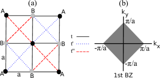
Figure 1: (color online) Sketches of (a) the crystal structure together with the hopping parameters in the real space, and (b) the corresponding first Brillouin zone in the reciprocal space.

To describe the hopping kinematics of the single-particle problem on such a lattice, we choose the primitive lattice vectors $\mathbf{a_{1}}=(a,-a)$ and $\mathbf{a_{2}}=(a,a)$ together with a basis of two sites. We are particularly interested in the competition between the following hopping parameters: if the location of a given site on the $A$ sublattice is $(0,0)$ then the intersublattice hopping $t$ connects it to the nearest-neighbor sites $\{(\pm a,0),(0,\pm a)\}$ on the $B$ sublattice, and the intrasublattice ones $t^{\prime}$ and $t^{\prime\prime}$ connect it to the next-nearest-neighbor sites $\{(a,a),(-a,-a)\}$ and $\{(a,-a),(-a,a)\}$, respectively, on the $A$ sublattice. In this paper, we assume $t>0$ and $t^{\prime}>t^{\prime\prime}\geq 0$ without loss of generality. The corresponding reciprocal lattice vectors $\mathbf{b_{1}}=(\pi/a,-\pi/a)$ and $\mathbf{b_{2}}=(\pi/a,\pi/a)$ give rise to the first Brillouin zone that is sketched in Fig. 1(b).

Depending on the interplay of these hopping parameters, such a crystal structure is known to exhibit two single-particle energy bands with very special features, e.g., an energetically flat band that shares quadratic touching points with a dispersive band in the reciprocal space, as discussed next.

II.1 Mean-field Hamiltonian

In the reciprocal space, the hopping contribution to the Hamiltonian can be written as $H_{0}=\sum_{\mathbf{\sigma k}}\psi_{\sigma\mathbf{k}}^{\dagger}h_{\mathbf{k}}\psi_{\sigma\mathbf{k}},$ where $\psi_{\sigma\mathbf{k}}^{\dagger}=(c_{\sigma A\mathbf{k}}^{\dagger}\,c_{\sigma B\mathbf{k}}^{\dagger})$ is the creation operator for a two-component sublattice spinor, and

$$h_{\mathbf{k}}=d_{\mathbf{k}}^{0}\tau_{0}+\mathbf{d_{\mathbf{k}}}\cdot\boldsymbol{\tau}$$ (1)

is the Hamiltonian density with $\tau_{0}$ a unit matrix, $\boldsymbol{\tau}=(\tau_{x},\tau_{z})$ a vector of Pauli matrices, and $\mathbf{d_{k}}=(d_{\mathbf{k}}^{x},d_{\mathbf{k}}^{z}).$ While the diagonal elements of $h_{\mathbf{k}}$ are due solely to the next-nearest-neighbor hoppings, the off-diagonal elements are due to the nearest-neighbor ones in such a way that

$$d_{\mathbf{k}}^{0} =-2(t^{\prime}+t^{\prime\prime})\cos(k_{x}a)\cos(k_{y}a),$$ (2)

$$d_{\mathbf{k}}^{x} =-2t\cos(k_{x}a)-2t\cos(k_{y}a),$$ (3)

$$d_{\mathbf{k}}^{z} =2(t^{\prime}-t^{\prime\prime})\sin(k_{x}a)\sin(k_{y}a).$$ (4)

The single-particle energy bands are determined by $\varepsilon_{s\mathbf{k}}=d_{\mathbf{k}}^{0}+sd_{\mathbf{k}},$ where $s=\pm$ denotes the upper/lower band and $d_{\mathbf{k}}=|\mathbf{d_{k}}|$. These bands touch each other at the following points $\mathbf{k}\equiv\{(\pm\pi/a,0),(0,\pm\pi/a)\}$ in the reciprocal space, i.e., at the four corners of the first Brillouin zone, where $d_{\mathbf{k}}=0$ and $\varepsilon_{s\mathbf{k}}=2(t^{\prime}+t^{\prime\prime})$. In particular when $t^{\prime}=t>t^{\prime\prime}=0$, the band structure reduces to $\varepsilon_{+,\mathbf{k}}=2t$ and $\varepsilon_{-,\mathbf{k}}=-2t-4t\cos(k_{x}a)\cos(k_{y}a),$ and therefore, a flat upper band that shares quadratic touching points with a dispersive lower band emerges. This is known to be one of the simplest two-band lattice models exhibiting a flat band.

For a given relation between the hopping parameters, the relative positions of these bands together with some of their important features are sketched in Fig. 2. For instance, when $t>t^{\prime}+t^{\prime\prime}$, sketch 2(a) implies that the upper band edges of the lower band touch to the local band minima of the upper band at the energy $2(t^{\prime}+t^{\prime\prime})$. The band width $4(t-t^{\prime})$ of the upper band is narrow compared to that $4(t+t^{\prime}+t^{\prime\prime})$ of the lower band. Thus, when $t>t^{\prime}>t^{\prime\prime}=0$, the upper band edges of the lower band touch precisely to the lower band edges of the upper band at the energy $2t^{\prime}$. On the other hand, when $t\leq t^{\prime}+t^{\prime\prime}$, sketch 2(b) implies that the upper band edges of the lower band touch to the upper band edges of the upper band at the energy $2(t^{\prime}+t^{\prime\prime})$. Since the band width $4t^{\prime\prime}$ of the upper band is controlled independently of that $8t$ of the lower band, an energetically quasi-flat upper band eventually appears in the $t^{\prime\prime}/t\to 0$ limit.

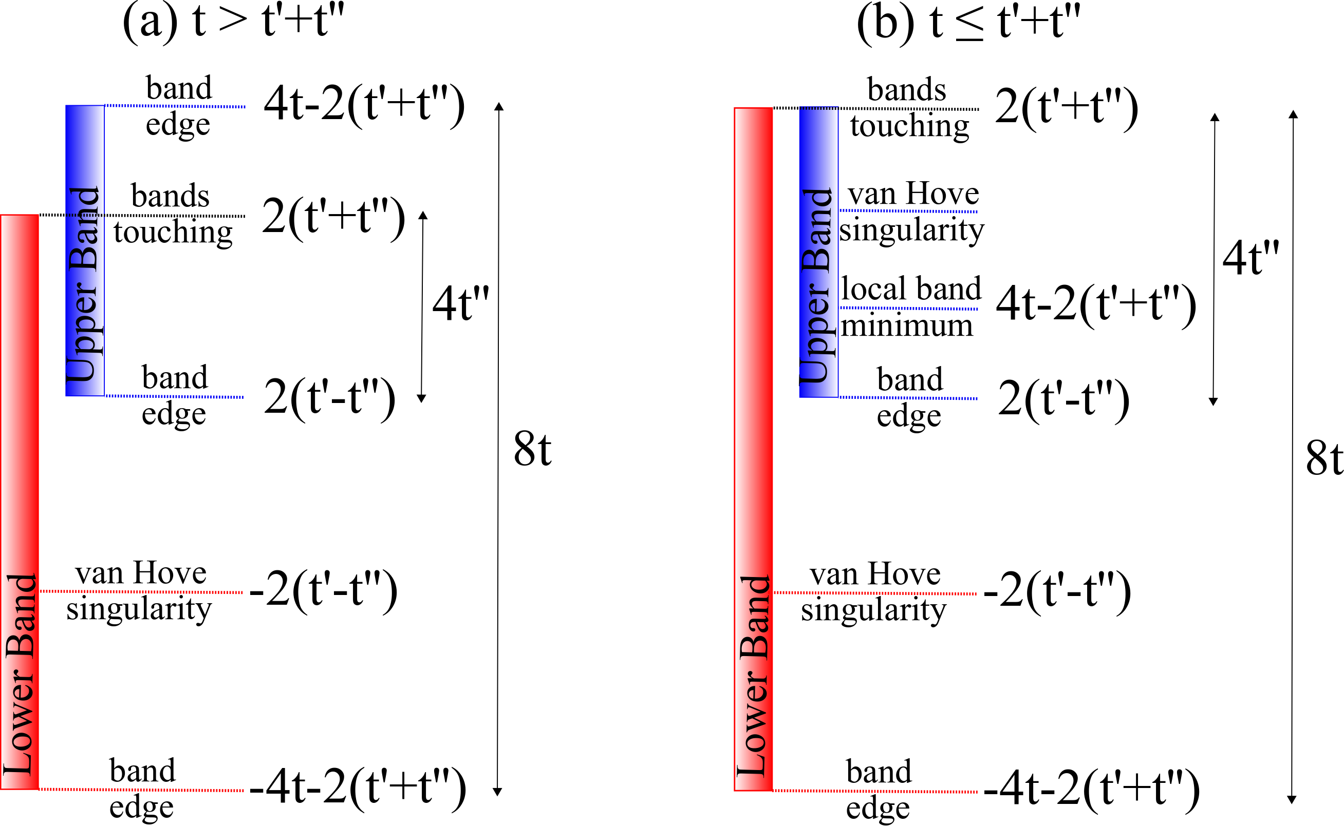
Figure 2: (color online) Sketches of the single-particle bands depending on whether the hopping parameters are related to each other through $t>t^{\prime}+t^{\prime\prime}$ or not. Here, and throughout this paper, we assume $t^{\prime}>t^{\prime\prime}\geq 0$ without loss of generality.

In direct analogy with the recent works torma17a ; iskin17 ; iskin18b ; iskin19 , the $\mathbf{k}$-space structure of $\mathbf{d_{k}}$ suggests that the quantum geometry of the reciprocal space is nontrivial as long as $t^{\prime}\neq t^{\prime\prime}$ for a given $t\neq 0$, i.e., the quantum metric tensor plays an important role in the formation of Cooper pairs and the related phenomena. To illustrate the quantum metric effects on the many-body problem, here we consider the case of attractive onsite interactions between $\uparrow$ and $\downarrow$ particles, and take them into account within the BCS mean-field approximation for pairing. The resultant Hamiltonian for the stationary Cooper pairs can be written as

$$H_{\textrm{mf}} =\sum_{\mathbf{k}}\Psi_{\mathbf{k}}^{\dagger}\left(\begin{array}[]{cc}h_{\mathbf{k}}-\mu\tau_{0}&\boldsymbol{\Delta}\\ \boldsymbol{\Delta}^{\dagger}&-h_{-\mathbf{k}}^{*}+\mu\tau_{0}\\ \end{array}\right)\Psi_{\mathbf{k}}$$ (7)

$$+2\sum_{\mathbf{k}}(d_{0}^{\mathbf{k}}-\mu)+M\frac{\Delta^{2}}{U},$$ (8)

where $\Psi_{\mathbf{k}}^{\dagger}=(\psi_{\uparrow\mathbf{k}}^{\dagger}\,\psi_{\downarrow,-\mathbf{k}})$ is a four-component spinor operator, $\boldsymbol{\Delta}_{SS^{\prime}}=\Delta_{S}\delta_{SS^{\prime}}$ is the order parameter with $\delta_{ij}$ the Kronecker-delta, $\mu$ is the chemical potential, $M$ is the number of lattice sites, and $U\geq 0$ is the strength of the interaction. It turns out that $\Delta_{S}=(2U/M)\sum_{\mathbf{k}}\langle c_{\downarrow S,-\mathbf{k}}c_{\uparrow S\mathbf{k}}\rangle$ with $\langle\ldots\rangle$ denoting the thermal average is uniform for the entire lattice, and we take $\Delta=\Delta_{S}$ as real without loss of generality.

II.2 Self-consistency equations

Given the mean-field Hamiltonian above by Eq. (8), a compact way to express the resultant self-consistency (order parameter and number) equations are iskin19 ,

$$1 =\frac{U}{2M}\sum_{s\mathbf{k}}\frac{\mathcal{X}_{s\mathbf{k}}}{E_{s\mathbf{k}}},$$ (9)

$$F =1-\frac{1}{M}\sum_{s\mathbf{k}}\frac{\mathcal{X}_{s\mathbf{k}}}{E_{s\mathbf{k}}}\xi_{s\mathbf{k}},$$ (10)

where $\xi_{s\mathbf{k}}=\varepsilon_{s\mathbf{k}}-\mu$ is the shifted dispersion, $\mathcal{X}_{s\mathbf{k}}=\tanh[E_{s\mathbf{k}}/(2T)]$ is a thermal factor with $k_{\textrm{B}}\to 1$ the Boltzmann constant and $T$ the temperature, $E_{s\mathbf{k}}=\sqrt{\xi_{s\mathbf{k}}^{2}+\Delta^{2}}$ is the quasi-particle energy spectrum, and $0\leq F=N/M\leq 2$ is the total particle filling with $N=\sum_{\sigma S\mathbf{k}}\langle c_{\sigma S\mathbf{k}}^{\dagger}c_{\sigma S\mathbf{k}}\rangle$ the total number of particles. Thus, the naive BCS mean-field theory corresponds to the self-consistent solutions of Eqs. (9) and (10) for $\Delta$ and $\mu$ for any given set of model parameters $t^{\prime}$, $t^{\prime\prime}$, $U$, $F$, and $T$. For instance, the critical BCS transition temperature $T_{\textrm{BCS}}$ is determined by the condition $\Delta\to 0^{+}$, and it gives a reliable estimate for the critical SF transition temperature in the weak-binding regime where $U\ll W$. Here, $W$ is the band width of the relevant band for pairing. This is in sharp contrast with the strong-binding regime, for which $T_{\textrm{BCS}}\propto U$ is known to characterize not the critical SF transition temperature but the pair formation one when $U\gg W$, i.e., the naive BCS mean-field theory breaks down.

The standard approach to circumvent this long-known difficulty is to include the fluctuations of the order parameter on top of the BCS mean-field in such a way that the critical SF transition temperature is determined by the universal BKT relation through an analogy with the XY model b ; kt ; nk . Such an analysis has recently been carried out for a class of two-band Hamiltonians, including the model of interest here torma17a . A compact way to express the resultant universal BKT relation is torma17a ; iskin17 ; iskin19 ,

$$T_{\textrm{BKT}} =\frac{\pi}{8}\sqrt{\det{\boldsymbol{D}}},$$ (11)

$$\boldsymbol{D}_{\mu\nu}^{\textrm{conv}} =\frac{\Delta^{2}}{\mathcal{A}}\sum_{s\mathbf{k}}\left(\frac{\mathcal{X}_{s\mathbf{k}}}{E_{s\mathbf{k}}^{3}}-\frac{\mathcal{Y}_{s\mathbf{k}}}{2TE_{s\mathbf{k}}^{2}}\right)\frac{\partial\xi_{s\mathbf{k}}}{\partial k_{\mu}}\frac{\partial\xi_{s\mathbf{k}}}{\partial k_{\nu}},$$ (12)

$$\boldsymbol{D}_{\mu\nu}^{\textrm{geom}} =\frac{2\Delta^{2}}{\mathcal{A}}\sum_{s\mathbf{k}}\frac{d_{\mathbf{k}}\mathcal{X}_{s\mathbf{k}}}{s(\mu-d_{\mathbf{k}}^{0})E_{s\mathbf{k}}}\boldsymbol{g}_{\mu\nu}^{\mathbf{k}},$$ (13)

where the tensor $\boldsymbol{D}=\boldsymbol{D}^{\textrm{conv}}+\boldsymbol{D}^{\textrm{geom}}$ corresponds to the SF phase stiffness, $\mathcal{A}$ is the area of the system, and $\mathcal{Y}_{s\mathbf{k}}=\mathrm{sech}^{2}[E_{s\mathbf{k}}/(2T)]$ is a thermal factor. The SF stiffness has two distinct contributions depending on the physical processes involved: while the intraband ones are called conventional, the interband ones are called geometric since only the latter is controlled by the total quantum metric tensor $\boldsymbol{g^{\mathbf{k}}}$ of the single-particle bands. A compact way to express its elements is resta11

$$\boldsymbol{g}_{\mu\nu}^{\mathbf{k}}=\frac{1}{2}\frac{\partial\widehat{\mathbf{d}}_{\mathbf{k}}}{\partial k_{\mu}}\cdot\frac{\partial\widehat{\mathbf{d}}_{\mathbf{k}}}{\partial k_{\nu}},$$ (14)

where $\widehat{\mathbf{d}}_{\mathbf{k}}=\mathbf{d}_{\mathbf{k}}/d_{\mathbf{k}}$ is a unit vector. Thus, the extended BCS mean-field theory corresponds to the self-consistent solutions of Eqs. (9), (10) and (11) for $\Delta(T_{\textrm{BKT}})$, $\mu(T_{\textrm{BKT}})$ and $T_{\textrm{BKT}}$ for any given set of model parameters $t^{\prime}$, $t^{\prime\prime}$, $U$, and $F$. In addition to reproducing the well-known BCS result for the weak-binding regime where $T_{\textrm{BKT}}\to T_{\textrm{BCS}}$ from below in the $U\ll W$ limit, this approach provides a reliable description of the strong-binding regime where $T_{\textrm{BKT}}\propto W^{2}/U$ in the $U\gg W$ limit.

II.3 Strongly-bound molecular pairs

Since $T_{\textrm{BKT}}\ll W\ll\Delta$ in the molecular regime, the self-consistency equations turn out to be analytically tractable, and their closed-form solutions provide considerable physical insight into the problem. For instance, the order parameter and number equations lead to $\Delta=(U/2)\sqrt{F(2-F)}$ and $\mu=-(U/2)(1-F).$ Similarly, the total SF stiffness reduces to $\boldsymbol{D}_{\mu\nu}=\{\Delta^{2}/[\mathcal{A}(\mu^{2}+\Delta^{2})^{3/2}]\}\sum_{\mathbf{k}}\textrm{Tr}\{(\partial h_{\mathbf{k}}/\partial k_{\mu})(\partial h_{\mathbf{k}}/\partial k_{\nu})\}$ with the trace Tr over the sublattice sector, and it is a diagonal matrix $\boldsymbol{D}_{\mu\nu}=D_{0}\delta_{\mu\nu}$ with an isotropic value $D_{0}=2\Delta^{2}(t^{2}+t^{\prime 2}+t^{\prime\prime 2})/(\mu^{2}+\Delta^{2})^{3/2}.$ Plugging these expressions into the universal BKT relation, we eventually obtain $T_{\textrm{BKT}}=\pi F(2-F)(t^{2}+t^{\prime 2}+t^{\prime\prime 2})/(2U),$ showing that $t^{\prime}$ and $t^{\prime\prime}$ increases $T_{\textrm{BKT}}$ for a given $F$ in the $U\gg t$ limit. Furthermore, we may relate $D_{0}$ to the density $\rho_{p}$ and effective mass $m_{p}$ of the SF pairs through the relation $D_{0}=4\hbar^{2}\rho_{p}/m_{p},$ where $\rho_{p}=F_{p}/a^{2}$ with $F_{p}$ the filling of SF pairs. To a good approximation, we may identify $F_{p}=F_{c}/2$ using the well-known expression leggett

$$F_{c}=\frac{\Delta^{2}}{2M}\sum_{s\mathbf{k}}\frac{\mathcal{X}_{s\mathbf{k}}^{2}}{E_{s\mathbf{k}}^{2}}$$ (15)

for the filling of condensed particles. In the strong-binding regime, this leads to $F_{p}\to F_{0}=F(2-F)/4$ as the filling of SF pairs whose effective mass $m_{p}=\hbar^{2}U/[4a^{2}(t^{2}+t^{\prime 2}+t^{\prime\prime 2})]$ increases with $U$ but decreases with $t^{\prime}$ and $t^{\prime\prime}$ in the $U\gg t$ limit. In the next section, these analytical expressions are used as a benchmark for our numerics, where we explore the solutions of the self-consistency equations as a function of $U$.

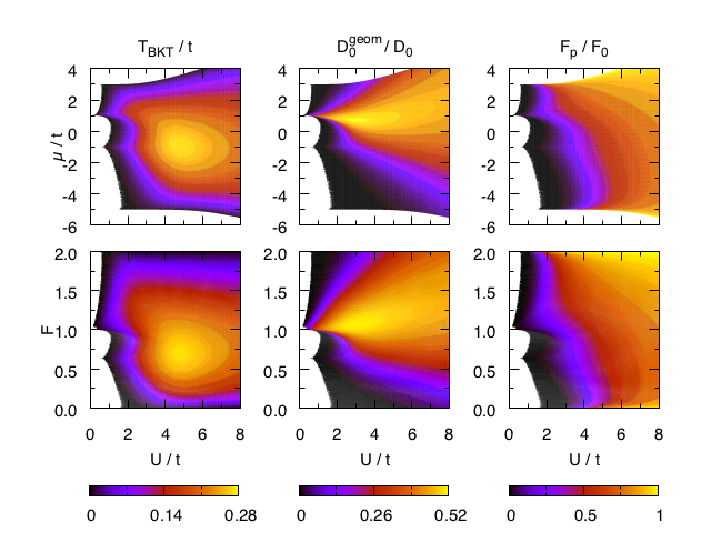
Figure 3: (color online) Left column is the critical SF transition temperature $T_{\textrm{BKT}}/t$, middle column is the relative weight $D_{0}^{\textrm{geom}}/D_{0}$ of the geometric SF stiffness, and right column is the faction $F_{c}/F_{0}$ of condensed particles. Here, the next-nearest-neighbor hoppings are $t^{\prime}=0.5t>t^{\prime\prime}=0$, corresponding to the sketch Fig. 2(a).

III Numerical Analysis

One of our main objectives in this paper is to study how the quantum geometry exposes itself in various SF properties through its contribution to the SF stiffness given above by Eq. (13). This expression suggests that a nonzero geometric contribution requires $t^{\prime}\neq t^{\prime\prime}$ for a given $t\neq 0$, which is simply because the band structure consists effectively of a single band when $t^{\prime}=t^{\prime\prime}$, and therefore, the interband processes necessarily vanish. Thus, for the sake of its conceptual simplicity, let us initially set one of the next-nearest-neighbor hopping parameters to zero, and consider $t^{\prime}=0.5t>t^{\prime\prime}=0$ as an example. Most important features for the corresponding single-particle problem can be extracted from the sketch Fig. 2(a), and the self-consistent solutions for the many-body problem are presented in Fig. 3.

First of all, having $t^{\prime}\neq 0$ splits the van Hove singularity of the usual square lattice model (for which the singularity lies precisely at $\mu=0$ or half filling $F=1$ when $t^{\prime}=t^{\prime\prime}=0$) into two, and produces one singularity per band. In Fig. 3, these singularities are clearly visible at $\mu=\pm t$, and the plus sign corresponds also to the energy at which the upper band edges of the lower band touch quadratically to the lower band edges of the upper band at $F=1$. In the $U/t\to 0$ limit, we note that the weakly-bound pairs first occupy the lower band for $-5t\leq\mu<t$ until it is full at $F=1$, and than they occupy the upper band for $t\leq\mu<3t$ until it is full at $F=2$. This figure reveals that it is the competition between these singularities that ultimately determines the critical SF transition temperature $T_{\textrm{BKT}}$ in the weak-binding regime, i.e., while $T_{\textrm{BKT}}$ is favored by the increase in the single-particle density of states near the van Hove singularity of the lower band, it is also enhanced by the geometric contribution to the SF stiffness emanating near the band edges/touchings. Since the band width $2t$ of the upper band is relatively much narrower than that $6t$ of the lower band, the geometric contribution plays a more decisive role for $F\gtrsim 1$. For completeness, the fraction $F_{p}/F_{0}$ of condensed particles is also shown in Fig. 3. In comparison to the half filling ($F=1$) where half of the pairs or holes may at most be condensed with $F_{0}\to 1/2$ in the strong-binding regime, all of the particle (hole) pairs are condensed with $F_{0}\to F/2$ ($F_{0}\to 1-F/2$) in the low particle (hole) filling $F\to 0$ ($F\to 2$) limit.

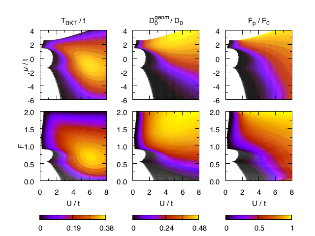
Figure 4: (color online) Same as in Fig. 3 but for $t^{\prime}=t$ and $t^{\prime\prime}=0.3t$, corresponding to the sketch Fig. 2(b).

Choosing a different value for $t^{\prime}<t$ does not change these results in any qualitative way, and that the competition between the contributions from the van Hove singularity of the lower band and the geometric SF stiffness near the band touchings always controls the weak-binding regime. This also turns out to be the case when both of the next-nearest-neighbor hoppings $t^{\prime}>t^{\prime\prime}\neq 0$ are at play. For instance, the self-consistent solutions for the $t^{\prime}=t$ and $t^{\prime\prime}=0.3t$ case are shown in Fig. 4 as an example. Most important features for the single-particle problem can be extracted from the sketch Fig. 2(b). In the $U/t\to 0$ limit, we find that the weakly-bound pairs first occupy the lower band for $-6.6t\leq\mu<1.4t$ until $F\approx 0.92$, and than they occupy both bands for $1.4t\leq\mu<2.6t$ until they are full at $F=2$. While the van Hove singularity of the lower band is clearly seen at $\mu=-1.4t$ or $F\approx 0.55$, that of the upper band is barely visible around $\mu\approx 1.62t$ or $F\approx 1.23$. In comparison to Fig. 3, since the band width $1.2t$ of the upper band is much narrower than that $8t$ of the lower band, and it lies fully within the energy interval of the latter, the geometric contribution plays an even more decisive role for $F\gtrsim 0.9$. In addition, having $t^{\prime\prime}\neq 0$ also increases the maximal $T_{\textrm{BKT}}/t$, which is in agreement with the analysis given above in Sec. II.3.

Given our sketches above in Figs. 2(a) and 2(b) for the single-particle bands depending on whether the hopping parameters are related to each other through $t>t^{\prime}+t^{\prime\prime}$ or not, it is possible to reach qualitative conclusions for other parameter sets including the flat-band limit when $t=t^{\prime}>t^{\prime\prime}=0$. However, motivated by the growing interest in understanding the origins of flat-band superfluidity in various other contexts discussed above in Sec. I, next we present an in-depth analysis showing how the flat-band superfluidity prevails in our model.

IV Flat-Band Superfluidity

When $t\leq t^{\prime}+t^{\prime\prime}$, our sketch Fig. 2(b) implies that decreasing the ratio $t^{\prime\prime}/t$ flattens the upper band with respect to the lower one, turning it eventually to an energetically quasi-flat band in the $t^{\prime\prime}/t\to 0$ limit. Here, we first set $t=t^{\prime}>t^{\prime\prime}=0$ and analyze the so-called Mielke checkerboard lattice model mielke91 ; montambaux18 , and then gain more physical insight by studying an effective low-energy continuum model for it.

IV.1 Mielke checkerboard lattice model

As discussed in Sec. II.1, the band structure in the Mielke checkerboard lattice is simply determined by

$$\varepsilon_{+,\mathbf{k}} =2t,$$ (16)

$$\varepsilon_{-,\mathbf{k}} =-2t-4t\cos(k_{x}a)\cos(k_{y}a),$$ (17)

for which the van Hove singularity of the lower band is precisely at $\varepsilon=-2t$ or $F=0.5$. This is in such a way that the lower band lies within the energy interval $-6t\leq\varepsilon_{-,\mathbf{k}}<2t$, and its upper band edges touch to the flat band at the four corners of the first Brillouin zone. All of these features are clearly visible in the self-consistent solutions for the many-body problem that are presented in Fig. 5. In the $U/t\to 0$ limit, we find that the weakly-bound pairs first occupy the lower band for $-6t\leq\mu<2t$ until $F=1$, and than they occupy the upper band at $\mu=2t$ until it is full at $F=2$. Since the upper band is entirely flat, the geometric contribution dominates the parameter space for $F\gtrsim 1$ in especially the weak-binding regime.

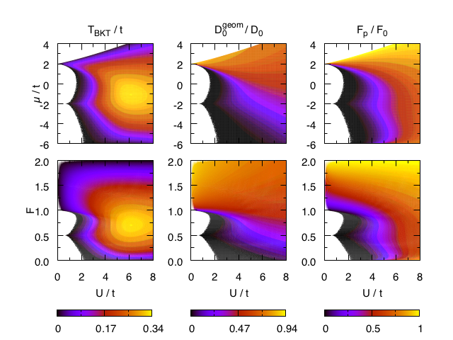
Figure 5: (color online) Same as in Fig. 3 but for $t^{\prime}=t>t^{\prime\prime}=0$, corresponding to a special limit in the sketch Fig. 2(b), i.e., for the so-called Mielke checkerboard lattice model discussed in Sec. IV.1.

Thanks to its analytical tractability, next we focus only on the $\mu=2t$ case, and reveal the origins of flat-band superfluidity as a function of $U/t$. For instance, when $\mu$ coincides with an isolated flat band at $U=0$ iskin17f , the ground state (i.e., at $T=0$ the zero temperature) is determined by $\Delta=(U/2)\sqrt{f(1-f)}$ and $\mu=2t+(U/2)(f-1/2)$ as soon as $U/t\neq 0$. Here, $0\leq f=F-1\leq 1$ is the filling of the isolated flat band for which $F_{c}=f(1-f)$ gives the filling of condensed particles. Thus, setting $\mu=2t$ in the $U/t\to 0$ limit, we find $f=1/2$, $\Delta=U/4$, $F=3/2$ and $F_{c}=1/4$, which are in perfect agreement with our numerics. Furthermore, our numerical calculations for the conventional contribution Eq. (12) to the SF stiffness $\boldsymbol{D}_{\mu\nu}^{\textrm{conv}}=(\Delta^{2}/\mathcal{A})\sum_{\mathbf{k}}(\partial\xi_{-,\mathbf{k}}/\partial k_{\mu})(\partial\xi_{-,\mathbf{k}}/\partial k_{\nu})/E_{-,\mathbf{k}}^{3}$ in the ground state fit perfectly well with $D_{0}^{\textrm{conv}}/(2F_{c})=U/(4\pi)$ when $\Delta/t\to 0$ in the $U/t\to 0$ limit. Similarly, the geometric contribution Eq. (13) to the SF stiffness $\boldsymbol{D}_{\mu\nu}^{\textrm{geom}}=(2\Delta/\mathcal{A})\sum_{\mathbf{k}}\boldsymbol{g}_{\mu\nu}^{\mathbf{k}}(1-\Delta/E_{-,\mathbf{k}})$ in the ground state fit extremely well (i.e., up to the machine precision) with $D_{0}^{\textrm{geom}}/(2F_{c})=U[\ln(64t/U)-1]/(4\pi)$ when $\Delta/t\to 0$ in the $U/t\to 0$ limit. In comparison, one can also calculate that $D_{0}^{\textrm{geom}}/(2F_{c})=D_{0}^{\textrm{conv}}/(2F_{c})=4t^{2}/U$ when $\Delta/t\gg 1$ in the $U/t\gg 1$ limit, which is in agreement with the analysis given above in Sec. II.3 where $F_{c}=F(2-F)/2\to 0.5$ in the $F\to 1$ limit when $\mu=2t$.

We also observe that the very same analytical expressions, i.e., $D_{0}^{\textrm{conv}}/(2F_{c})=U/(4\pi)$ for the conventional contribution and $D_{0}^{\textrm{geom}}/(2F_{c})=U[\ln(64t/U)-1]/(4\pi)$ for the geometric contribution, fit extremely well with the numerical results at $T=T_{\textrm{BKT}}$ in the $U/t\to 0$ limit. Here, $F_{c}$ also needs to be evaluated at $T_{\textrm{BKT}}$, for which Eq. (15) leads to $F_{c}\to 0$ when $\Delta/t\to 0$ in the $U/t\to 0$ limit. This observation is illustrated in Fig. 6, where we plot the self-consistent numerical solutions together with the analytical fits. We note that the $U$ dependence of the total SF stiffness $D_{0}/(2F_{c})=U\ln(64t/U)$ is very different from those $D_{0}/(2F_{c})\propto U$ of the isolated flat bands torma15 ; torma16 ; torma17a , which is one of the direct consequences of the band touchings as discussed below in Sec. IV.2.

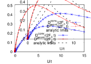
Figure 6: (color online) Conventional and geometric contributions to the SF stiffness for the Mielke checkerboard lattice model. Here, we set $t^{\prime}=t>t^{\prime\prime}=0$ and $\mu=2t$, and evaluate the contributions self-consistently at $T=T_{\textrm{BKT}}$.

The main physical reason behind the success of the very same fit at both $T=0$ and $T=T_{\textrm{BKT}}$ has to do with the effective mass $m_{p}$ of the strongly-bound molecular pairs. This is because, in accordance with the analysis given above in Sec. II.3, one may define the inverse of the effective pair-mass tensor $\boldsymbol{m_{p}}$ through plugging $\rho_{p}=F_{c}/(2a^{2})$ for the density of SF pairs in the relation

$$\boldsymbol{D}=4\hbar^{2}\rho_{p}\boldsymbol{m_{p}^{-1}}.$$ (18)

Thus, our analytical fits suggest that the effective mass of the pairs diverges as $m_{p}=4\pi\hbar^{2}/[Ua^{2}\ln(64t/U)]$ when $\mu=2t$ in the $U/t\to 0$ limit, which is directly caused by the diverging effective band mass of a single particle in a flat band. Furthermore, by separating the $\boldsymbol{D}$ and $\boldsymbol{m_{p}^{-1}}$ tensors into their conventional and geometric contributions, i.e., $(\boldsymbol{m_{p}^{-1}})_{\mu\nu}=(\boldsymbol{m_{p}^{-1}})_{\mu\nu}^{\textrm{conv}}+(\boldsymbol{m_{p}^{-1}})_{\mu\nu}^{\textrm{geom}},$ and using Eq. (13) along with the ground state parameters, we may also identify

$$(\boldsymbol{m_{p}^{-1}})_{\mu\nu}^{\textrm{geom}}=\frac{U}{\hbar^{2}M}\sum_{\mathbf{k}}\boldsymbol{g}_{\mu\nu}^{\mathbf{k}}\left(1-\frac{1}{\sqrt{1+\frac{16\xi_{-,\mathbf{k}}^{2}}{U^{2}}}}\right)$$ (19)

in the $U/t\to 0$ limit. This expression is almost identical to a very recent result torma19 where the inverse mass tensor of the two-body problem in an isolated flat band is reported as $(\boldsymbol{m_{p}^{-1}})_{\mu\nu}^{\textrm{geom}}=[U/(\hbar^{2}M)]\sum_{\mathbf{k}}\boldsymbol{g}_{\mu\nu}^{\mathbf{k}}.$ Since the Mielke flat band is not entirely isolated from the lower band, there is an extra term in Eq. (19) that cancels precisely those band touchings from the sum, i.e., when $\xi_{-,\mathbf{k}}\to 0$ in the $U/t\to 0$ limit. To show that the sum $\sum_{\mathbf{k}}\boldsymbol{g}_{\mu\nu}^{\mathbf{k}}$ by itself is infrared divergent for a flat band that is in touch with a dispersive one, next we construct a low-energy continuum model for the Mielke checkerboard lattice.

IV.2 Effective low-energy continuum model

For this purpose, we expand the single-particle Hamiltonian density $h_{\mathbf{k}}$ given above by Eqs. (1)-(4) near the band touchings, and arrive at its low-energy description where

$$d_{\mathbf{k}}^{0} =2t-t(k_{x}^{2}+k_{y}^{2})a^{2},$$ (20)

$$d_{\mathbf{k}}^{x} =-t(k_{x}^{2}-k_{y}^{2})a^{2},$$ (21)

$$d_{\mathbf{k}}^{z} =-2tk_{x}k_{y}a^{2}.$$ (22)

Then, the band structure is simply determined by $\varepsilon_{+,\mathbf{k}}=2t$ for the upper band and $\varepsilon_{-,\mathbf{k}}=2t-2tk^{2}a^{2}$ for the lower band, exhibiting a quadratic touching point at $\mathbf{k}=\mathbf{0}$ as sketched in Fig. 7. In addition, given that the band geometry is also characterized by a much simpler quantum metric tensor, i.e., Eq. (14) reduces to

$$\boldsymbol{g}_{\mu\nu}^{\mathbf{k}}=2\frac{k^{2}\delta_{\mu\nu}-k_{\mu}k_{\nu}}{k^{4}},$$ (23)

one can gain further physical insight by studying this continuum model at $\mu=2t$ in the $U/t\to 0$ limit.

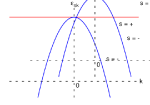
Figure 7: (color online) Band structure of the effective low-energy continuum model discussed in Sec. IV.2.

In perfect agreement with Sec. IV.1, the ground state is again determined by $\Delta=U/4$ and $F_{c}=1/4$, and we find $D_{0}^{\textrm{conv}}=\Delta/(2\pi)$ for the conventional contribution. Furthermore, we find that the infrared divergence of the sum $\sum_{\mathbf{k}}\boldsymbol{g}_{\mu\nu}^{\mathbf{k}}=[\mathcal{A}/(2\pi)]\ln(k_{\max}/k_{\min})\delta_{\mu\nu}$ is precisely cancelled by the infrared divergence of the sum $\Delta\sum_{\mathbf{k}}\boldsymbol{g}_{\mu\nu}^{\mathbf{k}}/E_{-,\mathbf{k}}=-[\mathcal{A}/(4\pi)]\ln(tk_{\min}^{2}a^{2}/\Delta)\delta_{\mu\nu},$ assuming $2tk_{\min}^{2}a^{2}\ll\Delta\ll 2tk_{\max}^{2}a^{2}$ in the $U/t\to 0$ limit. Here, $W=2tk_{\max}^{2}a^{2}$ is the band width of the lower band. Note that the analytical fit given above in Sec. IV.1 implies that $k_{\max}a\simeq 4/\sqrt{e}\approx 2.426.$ However, using the relation $\sum_{s\mathbf{k}}1=M$ for the number of lattice sites, we find $k_{\max}a=\sqrt{2\pi}\approx 2.507$ and $W=4\pi t$, leading eventually to $D_{0}^{\textrm{geom}}=[\Delta/(2\pi)]\ln[W/(2\Delta)].$ Thus, the low-energy model explains most of our findings in Sec. IV.1.

V Conclusions

To summarize, we exposed the quantum-geometric origin of flat-band superfluidity in the Mielke checkerboard lattice whose two-band band structure consists of an energetically flat band that is in touch with a quadratically dispersive one, i.e., a non-isolated flat band. For instance, in the weak-binding regime of arbitrarily low $U/t$, we found that the inverse effective mass tensor $\boldsymbol{m_{p}^{-1}}$ of the Cooper pairs is determined entirely by a $\mathbf{k}$-space sum over the so-called quantum metric tensor of the single-particle bands, leading to $m_{p}=4\pi\hbar^{2}/[Ua^{2}\ln(64t/U)]$ in the $U/t\to 0$ limit. Since the effective band mass of a non-interacting particle is infinite in a flat band, this particular result illuminates the physical mechanism behind how the mass of the SF carriers becomes finite with a finite interaction, i.e., how the quantum geometry is responsible for $m_{p}\neq\infty$ through interband processes as soon as $U/t\neq 0$. When $U/t$ increases from $0$, we also found that the geometric interband contribution gradually gives way to the conventional intraband one, eventually playing an equally important role in the strong-binding regime when $U/t\gg 1$.

Furthermore, given that $m_{p}$ plays direct roles in a variety of SF properties that are thoroughly discussed in this paper (i.e., the SF stiffness and critical SF transition temperature) but not limited to them (e.g., the sound velocity), this result also illuminates how the mean-field BCS correlations prevail in a non-isolated flat band. Curiously enough, such revelations of a fundamental connection between a physical observable and the underlying quantum geometry turn out to be quite rare in nature resta11 , making their cold-atom realization a gold mine for fundamental physics. We hope that our work motivates further research along these lines.

- (1) G.-B. Jo, J. Guzman, C. K. Thomas, P. Hosur, A. Vishwanath, and D. M. Stamper-Kurn, “Ultracold Atoms in a Tunable Optical Kagome Lattice”, Phys. Rev. Lett. 108, 045305 (2012).
- (2) Y. Nakata, T. Okada, T. Nakanishi, and M. Kitano, “Observation of flat band for terahertz spoof plasmons in a metallic kagomé lattice”, Phys. Rev. B 85, 205128 (2012).
- (3) Z. Li, J. Zhuang, L. Wang, H. Feng, Q. Gao, X. Xu, W. Hao, X. Wang, C. Zhang, K. Wu, S. X. Dou, L. Chen, Z. Hu, and Y. Du, “Realization of flat band with possible nontrivial topology in electronic Kagome lattice”, Science Advances 4, eaau4511 (2018).
- (4) S. Taie, H. Ozawa, T. Ichinose, T. Nishio, S. Nakajima, and Y. Takahashi, “Coherent driving and freezing of bosonic matter wave in an optical Lieb lattice”, Science Advances 1, e1500854 (2015)
- (5) F. Diebel, D. Leykam, S. Kroesen, C. Denz, and A. S. Desyatnikov “Conical Diffraction and Composite Lieb Bosons in Photonic Lattices”, Phys. Rev. Lett. 116, 183902 (2016).
- (6) S. Kajiwara, Y. Urade, Y. Nakata, T. Nakanishi, and M. Kitano, “Observation of a nonradiative flat band for spoof surface plasmons in a metallic Lieb lattice”, Phys. Rev. B 93, 075126 (2016).
- (7) H. Ozawa, S. Taie, T. Ichinose, and Y. Takahashi, “Interaction-Driven Shift and Distortion of a Flat Band in an Optical Lieb Lattice”, Phys. Rev. Lett. 118, 175301 (2017).
- (8) Z. Liu, F. Liu, and Yong-Shi Wu, “Exotic electronic states in the world of flat bands: from theory to material”, Chin. Phys. B 23, 077308 (2014).
- (9) D. Leykam, A. Andreanov, and S. Flach, “Artificial flat band systems: from lattice models to experiments”, Adv. Phys.: X 3, 1473052 (2018).
- (10) H. Tasaki, “From Nagaoka’s Ferromagnetism to Flat-Band Ferromagnetism and Beyond: An Introduction to Ferromagnetism in the Hubbard Model”, Prog. of Theoretical Physics 99, 489 (1998).
- (11) S. A. Parameswaran, R. Roy, and S. L. Sondhi, “Fractional Quantum Hall Physics in Topological Flat Bands”, Comptes Rendus Physique 14, 816 (2013).
- (12) V. A. Khodel and V. R. Shaginyan, “Superfluidity in systems with fermion condensate”, JETP Lett. 51, 553 (1990).
- (13) N. B. Kopnin, T. T. Heikkilä, and G. E. Volovik, “High-temperature surface superconductivity in topological flat-band systems”, Phys. Rev. B 83, 220503(R) (2011)
- (14) V. I. Iglovikov, F. Hébert, B. Grémaud, G. G. Batrouni, and R. T. Scalettar, “Superconducting transitions in flat-band systems”, Phys. Rev. B 90, 094506 (2014).
- (15) M. Tovmasyan, S. Peotta, L. Liang, P. Törmä, and S. D. Huber, “Preformed pairs in flat Bloch bands”, Phys. Rev. B 98, 134513 (2018).
- (16) R. Mondaini, G. G. Batrouni, and B. Grëmaud, “Pairing and superconductivity in the flat band: Creutz lattice”, Phys. Rev. B 98, 155142 (2018).
- (17) Y. Cao, V. Fatemi, S. Fang, K. Watanabe, T. Taniguchi, E. Kaxiras, and P. Jarillo-Herrero, “Unconventional superconductivity in magic-angle graphene superlattices”, Nature 556, 43 (2018).
- (18) M. Yankowitz, S. Chen, H. Polshyn, K. Watanabe, T. Taniguchi, D. Graf, A. F. Young, and C. R. Dean, “Tuning superconductivity in twisted bilayer graphene”, arXiv:1808.07865.
- (19) S. Peotta and P. Törmä, “Superfluidity in topologically nontrivial flat bands”, Nat. Com. 6, 8944 (2015).
- (20) A. Julku, S. Peotta, T. I. Vanhala, D.-H. Kim, and P. Törmä, “Geometric Origin of Superfluidity in the Lieb-Lattice Flat Band”, Phys. Rev. Lett. 117, 045303 (2016).
- (21) L. Liang, T. I. Vanhala, S. Peotta, T. Siro, A. Harju, and P. Törmä, “Band geometry, Berry curvature, and superfluid weight”, Phys. Rev. B 95, 024515 (2017).
- (22) P. Törmä, L. Liang, and S. Peotta, “Quantum metric and effective mass of a two-body bound state in a flat band”, Phys. Rev. B 98, 220511(R) (2018).
- (23) J. P. Provost and G. Vallee, “Riemannian structure on manifolds of quantum states”, Commun. Math. Phys. 76, 289 (1980).
- (24) M. V. Berry, “The quantum phase, five years after in Geometric Phases in Physics”, edited by A. Shapere and F. Wilczek (World Scientific, Singapore, 1989).
- (25) D. J. Thouless, “Topological Quantum Numbers in Nonrelativistic Physics”, (World Scientific, Singapore,1998)
- (26) M. Iskin, “Exposing the quantum geometry of spin-orbit coupled Fermi superfluids”, Phys. Rev. A 97, 063625 (2018).
- (27) M. Iskin, “Quantum metric contribution to the pair mass in spin-orbit-coupled Fermi superfluids”, Phys. Rev. A 97, 033625 (2018).
- (28) M. Iskin, “Superfluid stiffness for the attractive Hubbard model on a honeycomb optical lattice”, Phys. Rev. A 989, 023608 (2019).
- (29) A. Mielke, “Ferromagnetism in the Hubbard model on line graphs and further considerations”, J. Phys. A 24, 3311 (1991).
- (30) For a recent experimental proposal, see the supplemental material for G. Montambaux, L.-K. Lim, J.-N. Fuchs, and F. Piéchon, “Winding Vector: How to Annihilate Two Dirac Points with the Same Charge”, Phys. Rev. Lett. 121, 256402 (2018).
- (31) V. L. Berezinskii, “Destruction of long-range order in one-dimensional and two-dimensional systems having a continuous symmetry group I. classical systems”, JETP 32, 493 (1971).
- (32) J. M. Kosterlitz and D. J. Thouless, “Ordering, metastability and phase transitions in two-dimensional systems”, J. Phys. C: Solid State Phys. 6, 1181 (1973).
- (33) D. R. Nelson and J. M. Kosterlitz, “Universal Jump in the Superfluid Density of Two-Dimensional Superfluids”, Phys. Rev. Lett. 39, 1201 (1977).
- (34) R. Resta, “The insulating state of matter: a geometrical theory”, Eur. Phys. J. B 79, 121137 (2011).
- (35) A. J. Leggett, Quantum Liquids: Bose Condensation and Cooper Pairing in Condensed-Matter Systems (Oxford University Press, New York, 2006), Chap. 5.
- (36) M. Iskin, “Hofstadter-Hubbard model with opposite magnetic fields: Bardeen-Cooper-Schrieffer pairing and superfluidity in the nearly flat butterfly bands”, Phys. Rev. A 96, 043628 (2017).