Sparse Depth Enhanced Direct Thermal-infrared SLAM
Beyond the Visible Spectrum

Abstract

In this paper, we propose a thermal-infrared SLAM (SLAM) system enhanced by sparse depth measurements from LiDAR (LiDAR). Thermal-infrared cameras are relatively robust against fog, smoke, and dynamic lighting conditions compared to RGB cameras operating under the visible spectrum. Due to the advantages of thermal-infrared cameras, exploiting them for motion estimation and mapping is highly appealing. However, operating a thermal-infrared camera directly in existing vision-based methods is difficult because of the modality difference. This paper proposes a method to use sparse depth measurement for 6-DOF motion estimation by directly tracking under 14-bit raw measurement of the thermal camera. In addition, we perform a refinement to improve the local accuracy and include a loop closure to maintain global consistency. The experimental results demonstrate that the system is not only robust under various lighting conditions such as day and night, but also overcomes the scale problem of monocular cameras. The video is available at https://youtu.be/oO7lT3uAzLc.

I Introduction

Ego-motion estimation and mapping is a crucial factor for an autonomous vehicle. Much of the research in robotics has focused on imaging sensors and LiDAR [1, 2, 3] for navigating through environments without GPS (GPS). Conventional RGB cameras operating under the human visible spectrum hinder operating in a challenging environment such as fog, dust, and complete darkness. Recently, thermal-infrared cameras have been highlighted by studies for their perceptual capability beyond the visible spectrum and robustness to environmental changes.

Despite the outperformance against conventional RGB cameras, leveraging a thermal-infrared camera into previous visual perception approaches is a challenge in several respects. In particular, the distribution of data is usually low contrast because the temperature range sensed by a thermal-infrared camera is wider than the ordinary temperature range of daily life. In addition, due to the nature of thermal radiation, observable texture information in the human visible spectrum is lost and contrast is low in the images. To utilize previous approaches, a strategy of rescaling thermal images is used in [4, 5, 6, 7]. There are roughly two ways to rescale 14-bit raw radiometric data. First is to apply the histogram equalization technique using the full range of radiometric data present in the scene. However, performing a rescale using the entire range in this way causes a sudden contrast change if a hot or cold object suddenly appears. The change in contrast causes problems for both direct methods that require photometric consistency and feature-based methods that require thresholding for feature extraction. The second method is to manually set the range in which the rescale technique operates. Although there is a limitation to changing the range depending on the operating environment, this method maintains the photometric consistency according to the thermal condition. When a long-term operation is required, image degradation appears due to accumulated sensor noise and eventually deteriorates the performance of the SLAM[8].

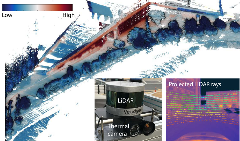
Figure 1: Sample 3D thermographic mapping result. Left thumbnail image shows the configuration of the thermal-lidar sensor system. Right thumbnail is the projected LiDAR points on the thermal image.

In this paper, we propose a direct thermal-infrared SLAM system enhanced by sparse range measurements. The proposed method tightly combines a thermal-infrared camera with a LiDAR to overcome the abovementioned challenges. Note that as shown in Fig. 1, only sparse measurement is available from the LiDAR. In addition, this sensor configuration solves the problem of initialization and scale of monocular SLAM approaches. However, precise calibration is required to utilize the two tightly coupled sensors. We achieve the calibration by utilizing the observable chessboard plane as a constraint in the thermal-infrared camera.

Inspired by direct methods [9, 1, 10], the proposed system tracks the sparse depth provided by LiDAR directly on the 14-bit raw thermal image. Unlike previous approaches that scale this 14-bit image to 8-bit, we utilize the raw temperature in 14-bit without conversion; doing so eliminates the heuristic preprocessing that rescales the value of the thermal image to 8-bit. Furthermore, we avoid applying RGB-D sensors based on structured IR (IR) patterns and obtain depth measurement that operates regardless of light condition from day to night.

The main characteristics of the proposed method can be explained as follows:

• We eliminate the heuristic preprocessing of the thermal imaging camera by tracking the sparse depth measurement on a 14-bit raw thermal image. Hence the high accuracy in the motion estimation stage can be guaranteed without geometric error models such as reprojection error of feature correspondences or ICP (ICP).

• The proposed method introduces a thermal image based loop-closure to maintain global consistency. When calculating the pose constraint, we consider the thermographic change from a temporal difference between the candidate keyframe and the current keyframe.

• Our system completes thermographic 3D reconstruction by assigning temperature values to points. The proposed method performs robustly regardless of day and night.

• Finally, experimental results show that a thermal-infrared camera with a depth measurement beyond the visible spectrum ultimately leads to an all-day visual SLAM.

II Related Works

During the last decade, vision-based motion estimation using consecutive images has matured into two main streams. One of them is a 6-DOF motion estimation method that utilizes visual feature correspondence [2, 11]. The other approach, called a direct method, estimates the ego-motion by minimizing the intensity difference of reprojected pixels from depth [9, 1, 12, 10]. It depends on visually rich information under sufficient lighting conditions.

The robustness of motion estimation under varying illumination is a critical issue for robotic applications. Due to the physical limitations of the generic imaging sensor, securing robustness of visual odometry methods under various lighting conditions (e.g., sunrise, sunset and night) has hardly been achieved [13]. In this respect, utilizing unconventional imaging sensors operatable under non-visible spectra has drawn attention.

Among them, thermal-infrared imaging has been highlighted. One approach introduces a method of visual and thermal-infrared image fusion based on DWT (DWT) and applies the representation to the visual odometry framework for the robustness in [5]. Another study suggested an odometry module that uses multi-spectral stereo matching instead of the fusion-based approach [6]. The authors used MI (MI) to perform cross-modality matching and temporal matching to improve matching accuracy. Instead of tightly fusing a multi-spectral sensor, a method of integrating each sensor’s measurement as a map point has also been introduced by [8]. Additionally, using thermal stereo for odometry module has been proposed for UAV (UAV) in [4].

In past decades, many studies on the 3D thermographic mapping have been introduced. Particularly in the remote sensing field, research has been conducted to integrate aerial thermal imagery and LiDAR data for ground survey and cities modeling [14, 15]. A thermographic mapping approach utilizing a terrestrial laser scanner has also been proposed instead of requiring expensive aerial equipment [16]. However, these methods have limitations in mobility because they require expensive equipment and have significantly lower portability.

Together with the real-time mobile 3D reconstruction [17, 18], portable mobile thermographic mapping methods have also been studied for building inspection [19, 20]. Since dense depth is available from an RGB-D sensor in their application, a geometric error model such as ICP was utilized. Recent studies have used the thermographic error model to improve robustness. More recently, methods have been introduced that combine thermographic error models to improve robustness [21, 22]. However, these methods that heavily rely on RGB-D sensors and are less suitable for an outdoor environment.

Targetting both indoor and outdoor, we take advantage of the direct visual-LiDAR SLAM method to our sensor system [23] and modify it to the newly proposed thermal-LiDAR system as shown in Fig. 1. In this paper, we summarize modifications and changes toward depth-enhanced direct SLAM for thermal cameras enabling all-day motion estimation and 3D thermographic mapping. The detailed topic includes 14-bit loss function for direct method, extrinsic calibration between a thermal camera and a LiDAR, and temperature bias correction during a loop-closure.

III Automatic Thermal Camera-to-LIDAR Calibration

In this section, we describe the estimation of the relative transformation $\mathbf{T}^{c}_{v}$ between the thermal camera coordinate frame $\{c\}$ and the LiDAR coordinate frame $\{v\}$ where two sensors are assembled as shown in Fig. 1. Given the initial transformation by hardware design, we optimize to obtain relative transformation between two sensors in terms of the extrinsic calibration parameters. The calibration accuracy is critical in the proposed method as a small calibration error may yield a large drift in the entire trajectory estimation.

Existing methods often aimed at estimating the relative pose between the RGB camera and the range sensor [24, 25, 26]. Even though the geometry of the thermal camera is similar to that of an RGB camera, these methods do not directly apply to our sensor system because the visible spectrum is completely different. The existing approaches for thermal-LiDAR extrinsic calibration [27, 28] require dense range data together with a user intervention for data selection. Instead, we propose an automated extrinsic calibration method that utilizes an observable chessboard pattern in the spectrum of a thermal-infrared camera, while requiring little user intervention. Using a pattern board that is visible to a thermal camera, we leverage a pattern board plane obtained from a data stream instead of using multiple planes in a single scene.

III-A Pattern Board

Pattern boards printed on generic paper are widely used in RGB camera calibration. However, they are only effective in the visible spectrum and reveal near-uniform radiation for a thermal camera. Hence, several chessboard patterns have been introduced to obtain intrinsic parameters of thermal cameras [28]. Inspired by these methods, we used a pattern board that utilizes a PCB (PCB). Because a conductive copper surface appears as a white region in a thermal camera image, we can use the conventional method of chessboard detection. This pattern board was used for both intrinsic and extrinsic calibration of thermal cameras.

III-B Plane segmentation

The purpose of segmentation in the calibration phase is to automatically find a pattern board and plane parameter from two sensors. The proposed method assumes that the initial extrinsic parameters can be obtained by hardware design.

Once the intrinsic parameters of the thermal camera and the size of the pattern have been given, we can easily estimate the chessboard pose in the camera coordinate system using existing methods [29]. Then, we detect the plane of the pattern board observed in the LiDAR coordinate system. Using the initial extrinsic parameter, we project the 3D points of the LiDAR coordinate system onto the thermal image. We use the plane-model based RANSAC algorithm using only those existing on the pattern board. As a result, we estimate plane models from the sparse points in the LiDAR coordinate system.

III-C Initial Parameter Estimation

The process of estimating extrinsic parameters between two sensors was inspired by [24]. Unlike [24], who utilized single shot data, we exploit a temporal data stream. Given a plane data pair from a LiDAR and a thermal camera, the relative transformation between the sensors is obtained using the geometric constraints of the plane model. Since the proposed method uses a temporal data stream in which a single chessboard is observed, the information from plane models, $ax+by+cz+d=0$, oriented in a similar direction becomes redundant. At least three plane models are required to calculate the transformation, and all possible combinations of selected indexes are precomputed. Among them, the algorithm selects three plane pairs ($p_{a},p_{b},p_{c}$) from the thermal camera to maximize the following probability:

$$\small p(s_{p_{a}},s_{p_{b}},s_{p_{c}})=\frac{1}{Z}\exp(-\mathbf{n}_{p_{a}}^{T}\mathbf{n}_{p_{b}}-\mathbf{n}_{p_{b}}^{T}\mathbf{n}_{p_{c}}-\mathbf{n}_{p_{a}}^{T}\mathbf{n}_{p_{a}}),$$ (1)

where $Z$ is the normalization factor, $s_{p_{a}},s_{p_{b}},s_{p_{c}}$ are the indices of the three selected plane pairs, and $\mathbf{n}$ is the normal of the plane. Intuitively, the greater the difference between the normals of the three planes, the higher the probability. Given three plane pairs, we solve the relative rotation of the two sensors via the equation below:

$$\operatorname*{argmax}_{\mathbf{R}^{v}_{c}}\sum_{i\in\{p_{a},p_{b},p_{c}\}}{\mathbf{n}^{i}_{v}}^{T}\mathbf{R}^{v}_{c}\mathbf{n}^{i}_{c}=\mathbf{V}\mathbf{U}^{T},$$ (2)

where the subscripts $c$ and $v$ indicate the coordinates of the camera and LiDAR. By performing SVD (SVD) of the covariance matrix $\sum_{i}{\mathbf{n}^{i}_{c}{\mathbf{n}^{i}_{v}}^{T}}=\mathbf{U}\Sigma\mathbf{V}^{T}$, the rotation matrix $\mathbf{R}^{v}_{c}$ estimation that maximizes the alignments of the normal vectors is calculated:

$$\operatorname*{argmin}_{\mathbf{t}}\sum_{i\in\{p_{a},p_{b},p_{c}\}}{\mathbf{n}^{i}_{v}}^{T}(\mathbf{R}^{v}_{c}\mathbf{p}^{i}_{c}+\mathbf{t}^{v}_{c})+d_{v}.$$ (3)

Next, we obtain a translational vector that minimizes the distance between a point found in the camera and a plane-model extracted from LiDAR.

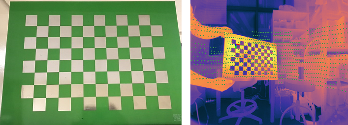
Figure 2: Pattern board and the calibration result. The green points represent lidar measurements projected onto a thermal image.

III-D Refinement

Following the previous section, the initial parameters were calculated using the normal and plane-to-point distances of the planes observed at each sensor. This method can be computed quickly in a closed form, but is less accurate and requires additional refinement. In this work, we use a gradient descent method to refine the relative transformation that minimizes the cost as following:

$$\operatorname*{argmin}_{\mathbf{R^{v}_{c}},\mathbf{t}}\sum_{i}{\mathbf{n}^{i}_{v}}^{T}(\mathbf{R}^{v}_{c}\mathbf{p}^{i}_{c}+\mathbf{t}^{v}_{c})+d_{v}.$$ (4)

At this stage, we use all plane data pairs obtained from the segmentation procedure mentioned in the previous section. Fig. 2 shows the calibration results by the proposed method. The points in the LiDAR coordinate system are projected into thermal camera images.

IV Sparse Depth Enhanced Direct Thermal-Infrared SLAM

Given an extrinsic calibration, we can project LiDAR points onto a thermal image frame. Fig. 3 provides the pipeline of the thermal-infrared SLAM. The proposed thermal-infrared SLAM method focuses on (i) accurate 6-DOF tracking of the direct method and (ii) a reliable loop detection method based on the visual features. The thermal-infrared SLAM consists of a tracking thread for estimating the 6-DOF motion of the input frame and a mapping thread for maintaining global consistency. We assume that the LiDAR and the thermal camera are already synchronized. Because depth measurements from LiDAR are available even in a sparse form, we are able to exploit the measurement instead of triangulating the corresponding points from the thermal-infrared camera.

The tracking thread directly estimates the relative motion by tracking the points of the previous frame and then performs pose refinement from multiple keyframes to improve local accuracy. We utilized the point sampling method for computational efficiency similar to [23]. By tracking the LiDAR depth measurement associated with the 14-bit raw thermal image, we can easily take advantage of the direct method. Note that we exploit only the sparse points within the camera FOV (FOV), suggesting potential application to a limited FOV LiDAR (e.g., solid-state LiDAR).

Lastly, the mapping thread aims to maintain global consistency. We utilized a bag-of-word-based loop detection when the current frame is revisited. However, the thermal images lack detailed texture information unlike the RGB images in the visible spectrum, thus naive implementation results in repetitive frequently detected pattern features and inaccurate loop candidates. Hence, we enforce the geometric verification to avoid adding incorrect loop constraints to the pose-graph.

IV-A Notation

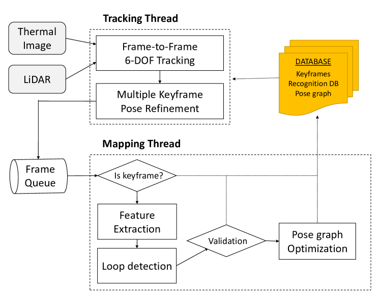
Figure 3: Block diagram of the direct thermal-infrared SLAM with sparse depth. The proposed method consists of a tracking module for estimating the pose of each frame and a loop closing module for global consistency.

A temperature image $\mathcal{I}_{i}$ and a sparse point cloud $\mathbf{\mathcal{P}}^{i}_{v}$ are provided via synchronization. Using the extrinsic parameters obtained in the previous section, we obtain the transformed point cloud $\mathbf{\mathcal{P}}^{i}_{c}$ in the camera coordinate. Then, each point $\mathbf{p}^{k}_{c}=(x,y,z)^{\top}\in\mathbb{R}^{3}$ is represented as a pixel $\mathbf{u_{k}}=(u,v)\in\mathbb{R}^{2}$ on the image coordinate system through the projection function $\pi(\mathbf{p}_{k})$ via

$$\mathbf{u_{k}}=\pi(\mathbf{p}_{k})=\left(\frac{xf_{x}}{z}+c_{x},\frac{yf_{y}}{z}+c_{y}\right).$$ (5)

The transformation matrix $\mathbf{T}_{n}\in SE(3)$ on the world coordinate represents the pose of each frame and the relative pose between $\mathcal{F}_{n}$ and $\mathcal{F}_{m}$ is denoted by $\mathbf{T}_{m}^{n}=\mathbf{T}_{n}^{-1}\mathbf{T}_{m}$. This relative pose is also used for the coordinate transformation of points as follows:

$$\mathbf{p}_{n}=\mathbf{T}_{m}^{n}\mathbf{p}_{m}=\begin{bmatrix}\mathbf{R}_{m}^{n}&\mathbf{t}_{m}^{n}\\ \mathbf{0}&1\end{bmatrix}\mathbf{p}_{m},$$ (6)

where $\mathbf{p}_{m}$ represent points on the frame $\mathcal{F}_{m}$, $\mathbf{R}_{m}^{n}\in SO(3)$ and $\mathbf{t}_{m}^{n}\in\mathbb{R}^{3}$ are a rotation matrix and translation vector. Lie algebra elements $\mathbf{\xi}\in\mathbb{R}^{6}$ are used as linearized pose increments. The twist $\xi=[\mathbf{w},\mathbf{v}]$ consist of an angular and linear velocity vector. The updated transformation matrix using the increment can be calculated by exponential mapping from Lie algebra to Lie group: $se(3)\times SE(3)\rightarrow SE(3)$, i.e.,

$$\mathbf{\mathrm{bar}{T}}_{m}^{n}=\exp(\hat{\xi})\mathbf{T}_{m}^{n}.$$ (7)

IV-B Tracking

Inspired by recent direct methods [1, 10], our tracking method utilizes a thermographic error model. Instead of a photometric error model that utilizes the intensity of the image, we use the 14-bit temperature value provided by the thermal-infrared camera. Additionally, we apply a patch $\Omega$ of the sparse pattern to ensure robustness as in [10]. Although this patch-based approach requires more computation, it provides robust results for image degradation such as motion blur or noise.

In the tracking process, the points $\mathbf{p}_{m}$ of the $m^{\text{th}}$ frame can be projected onto the image $\mathcal{I}_{n}$ of the current frame $\mathcal{F}_{n}$ by the initial relative pose. Thermographic residuals are expressed as the difference in temperature value as shown below

$$r(\mathbf{p}_{m})=\mathcal{I}_{n}(\pi(\mathbf{T}_{m}^{n}\mathbf{p}_{m}))-\mathcal{I}_{m}(\pi(\mathbf{p}_{m})).$$ (8)

Finally, our objective function for tracking is defined as follow:

$$\mathit{E}_{track}=\sum_{\mathbf{p}\in\Omega}w(r(\mathbf{p}))(r(\mathbf{p}))^{2},$$ (9)

where $\Omega$ is the patch of the sparse pattern and the function $w(\cdot)$ is a weight function based on the t-distribution, which is calculated iteratively and recursively as shown in [9, 23]:

$$w(r)=\frac{\nu+1}{\nu+(\frac{r}{\sigma_{r}})^{2}},$$ (10)

where $\nu$ is the degree of freedom, which was set to five, and the variance of residual $\sigma_{r}$ is iteratively estimated while performing the Gauss-Newton optimization algorithm. The effect of weighting is reported in [9]. Finally, a coarse-to-fine scheme is used to prevent large displacements that cause a local minimum of the cost function.

IV-C Local Refinement

In the previous section, the tracking process estimates 6-DOF relative motion by frame-to-frame. When the time interval between frames is short, tracking loss and potential local drift inevitably occur. To reduce this drift and improve local accuracy, we perform a multiple keyframe-based refinement. Once the frame-to-frame tracking process is completed, we perform optimization using the recent keyframes. The main difference with the tracking process is that optimization is performed on map coordinates based on multiple keyframes.

Given that the poses of the keyframes are defined in the map coordinate, we update the current frame pose using the relative motion obtained from the tracking process prior to the refinement phase using the cost below:

$$\mathit{E}_{refine}=\sum_{\mathcal{KF}_{i}\in\mathbf{W}_{kf}}\sum_{\mathbf{p}_{k}\in\mathbf{P}_{\mathbf{i}}}\sum_{\mathbf{p}_{k}\in\Omega}w(r(\mathbf{p}_{k}))(r(\mathbf{p}_{k}))^{2},$$ (11)

where $\mathbf{W}$ represents the window of multiple keyframes, $\mathbf{p}$ indicates the points of the keyframe and $\Omega$ means the patch of the sparse pattern. The weight function $w(\cdot)$ uses t-distribution, as described in the previous section. The residual function $r(\cdot)$ is defined using the raw values of the keyframe and the current frame as:

$$r(\mathbf{p}_{m})=\mathcal{I}_{f}(\pi(\mathbf{T}_{f}^{-1}\mathbf{T}_{kf}\mathbf{p}_{k}))-\mathcal{I}_{kf}(\pi(\mathbf{p}_{k})).$$ (12)

Lastly, the equation (11) is optimized with respect to the pose of the current frame using the Gauss-Newton method.

IV-D Loop Closing

IV-D1 Loop Detection

The inferred thermal odometry estimation may deteriorate the global consistency due to the accumulation of small drifts and errors. We handle this issue by relying on a loop closure that takes advantage of the constraints between the revisited place and the current frame. In the mapping thread, detection of the revisiting area depends on DBoW, a place recognition method based on the bag-of-binary-words [30].

Each time a new keyframe is created, we extract the ORB feature from the thermal image. Instead of directly utilizing the 14-bit raw data for loop closure, we chose a strategy that performs equalization through a linear operation in a fixed range of ordinary temperature ($0^{\circ}$ to $30^{\circ}$). Because only the simple linear operation is required, we can expect the applicability of the feature extraction methodology to 14-bit raw data.

Next, we calculate the bag-of-words vectors then calculate the normalized similarity score from the keyframe database.

$$\eta(\mathbf{v}_{c},\mathbf{v}_{q})=\frac{s(\mathbf{v}_{c},\mathbf{v}_{q})}{s(\mathbf{v}_{c},\mathbf{v}_{1})}$$ (13)

where $\mathbf{v}_{q}$ is the BoW vector of the previous keyframes. To calculate the similarity score $s(\mathbf{v}_{c},\mathbf{v}_{q})$, the $L_{1}$ distance is used as shown below:

$$s(\mathbf{v}_{c},\mathbf{v}_{q})=1-\frac{1}{2}\left|\frac{\mathbf{v}_{c}}{|\mathbf{v}_{c}|}-\frac{\mathbf{v}_{q}}{|\mathbf{v}_{q}|}\right|$$ (14)

Since keyframes are added sequentially while excluding keyframes with a timestamp close to the current frame from the loop candidate, an additional check on the ratio of common words is performed to prevent false positives.

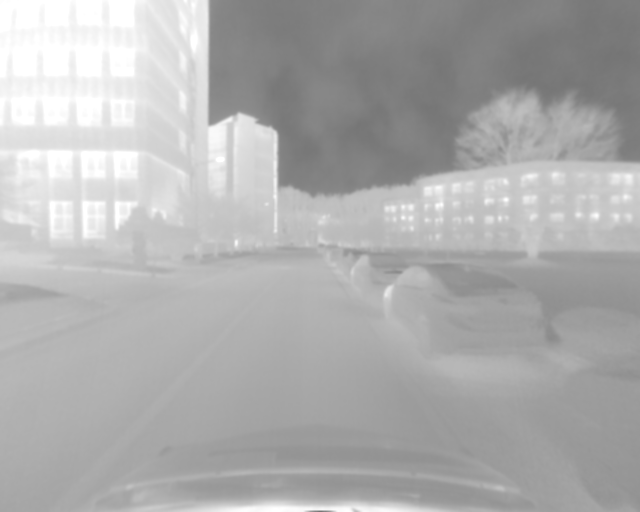
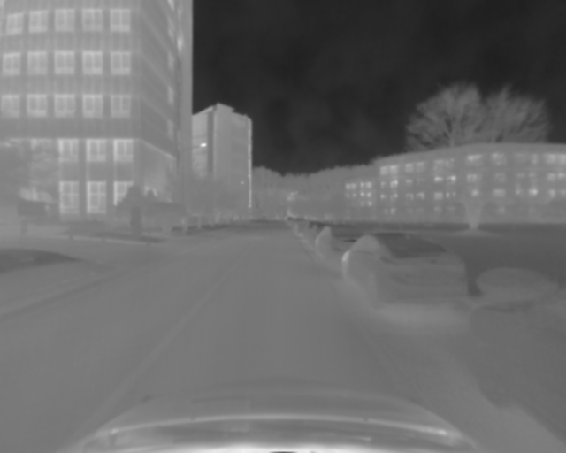
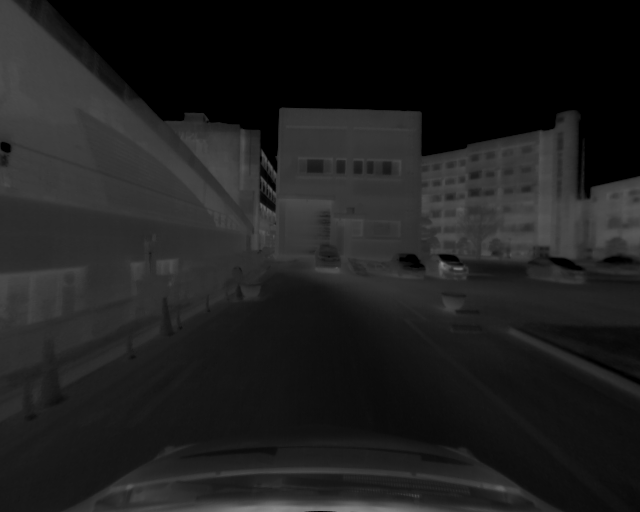
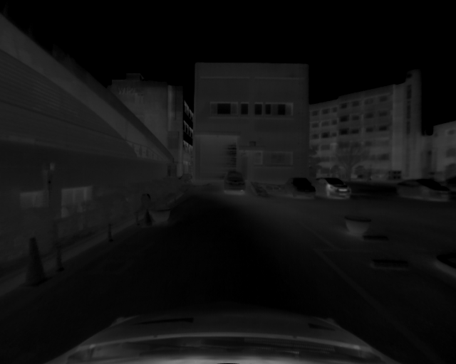
Figure 4: Example of inconsistency due to temporal difference between loop candidate keyframe and query frame. The left column is the query frame and the right image is the image of the revisited keyframe found. Note the image intensity (temperature) difference over time.

IV-D2 Loop Correction

When a candidate keyframe $\mathcal{F}_{kf}$ is detected for the loop-closure, we perform cross-validation by calculating each relative pose using the points owned by the current frame $\mathcal{F}_{c}$ and the candidate keyframe $\mathcal{F}_{kf}$. Given a current frame $\mathcal{F}_{c}$ and a candidate keyframe $\mathcal{F}_{kf}$, we estimate two relative motions $\mathbf{T}^{kf}_{c}$ and $\mathbf{T}^{c}_{kf}$.

Another notable phenomenon in operating thermal visual odometry outdoors is the gradual shift in the temperature during a mission. When a significant temporal difference between the two frames occurred, the consistency of the two images collapsed. As shown in Fig. 4, unlike RGB images that rarely change within an hour, we notice that the temperature may reveal substantial bias over a relatively short period of time. Therefore, the conventional relative motion estimation using the residual model as in RGB images is aggravated. To cope with this difference in the thermal images, we used an affine illumination model from [31].

$$r(\mathbf{p}_{ref})=(a\mathcal{I}_{n}(\pi(\mathbf{T}_{ref}^{n}\mathbf{p}_{ref}))+b)-\mathcal{I}_{ref}(\pi(\mathbf{p}_{ref})).$$ (15)

Above, the residual model applies to (9) and can be solved iteratively. However, the parameters $a$ and $b$ for the affine illumination model are known to react differently to outliers with the 6-DOF motion parameter $\xi$ from [32]. We applied an alternative optimization method to disjointly solve $a$ and $b$ in an iterative optimization process.

$$\left\lVert{\log{\left(\mathbf{T}_{kf}^{c}\mathbf{T}_{c}^{kf}\right)}}\right\rVert<\epsilon$$ (16)

When two relative poses are obtained, we lastly check the consistency between the two estimates prior to adding the loop-closure to the pose-graph. If the difference between the two relative pose estimates is smaller than the threshold $\epsilon$ in (16), a loop constraint is added to the pose graph and the correction is performed.

V Experimental Results

The proposed method was validated using a sensor system with rigidly coupled LiDAR and a thermal-infrared camera as shown in Fig. 1. The detailed specifications of the sensors that make up the system are shown in Table. I. An A65 thermal camera from FLIR was used in the experiment. The camera senses the spectral range in the LWIR (LWIR) region and provides 14-bit raw images with a $90^{\circ}$ of horizontal FOV.

TABLE I: Specifications of thermal camera and LiDAR

Type	Manufacturer	Model	Description
Thermal Camera	FLIR	A65	$90^{\circ}\times 69^{\circ}$ FOV with 7.5mm lens 7.5 $\sim$13 um spectral range (LWIR) 14-bit 640x512 resolution @ 30Hz $-40^{\circ}$ to $550^{\circ}$ temperature range
3D LiDAR	Velodyne	VLP-16	16 channel $360^{\circ}$ FOV @ 5$\sim$20Hz measurement range up to 100m

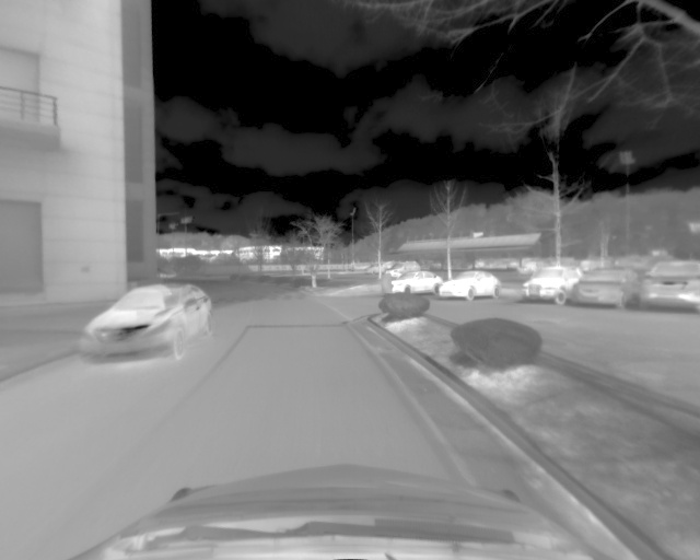
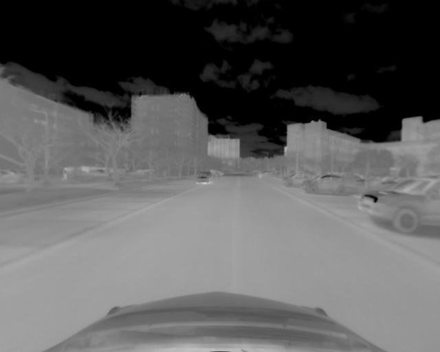
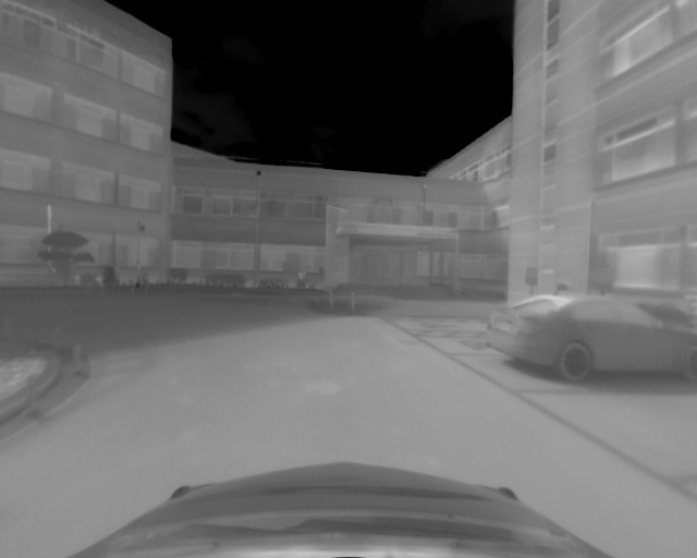
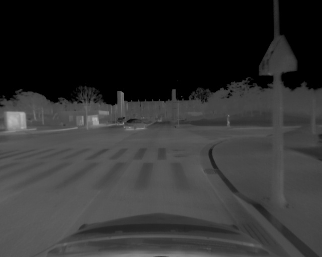
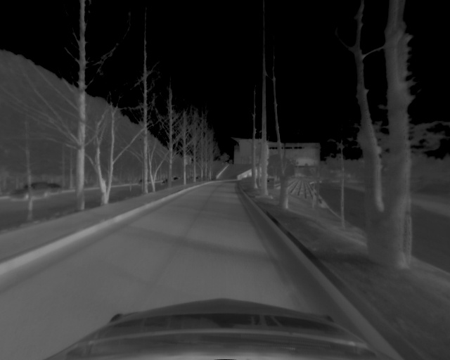
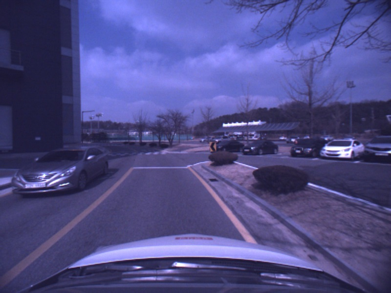
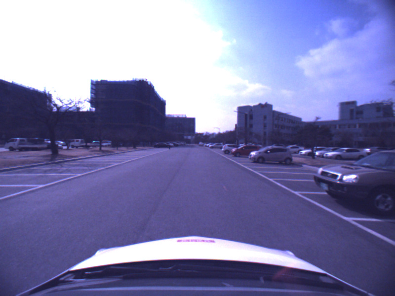
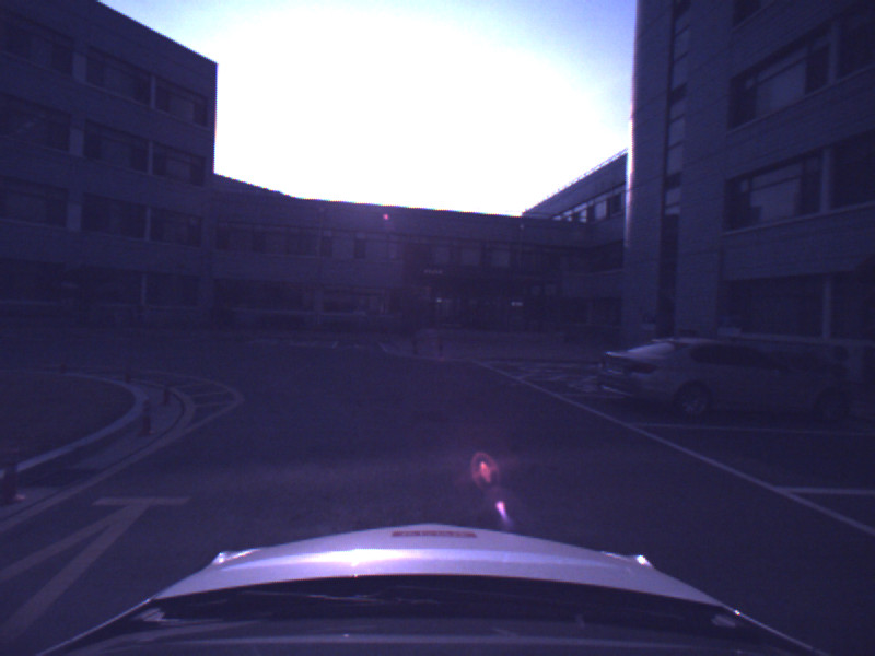
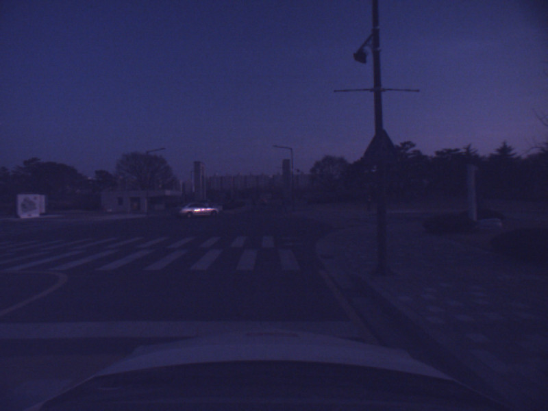
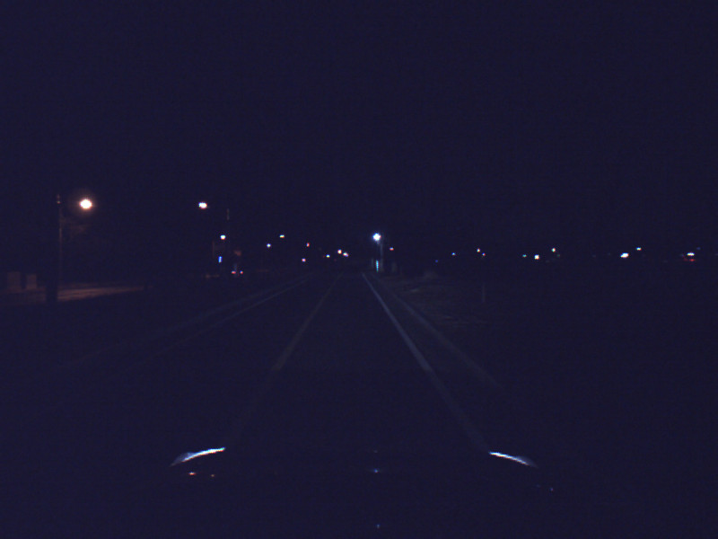
Figure 5: Sample thermal-infrared images (first row) and RGB images (second row). Unlike RGB images, thermal images are clearly captured regardless of light condition (day or night).

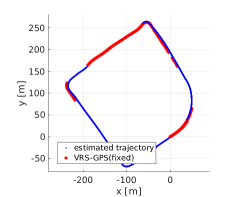
(a) Seq 9

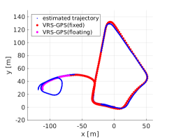
(b) Seq 11

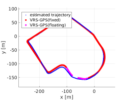
(c) Seq 14

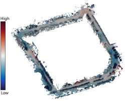
(d) Map 9

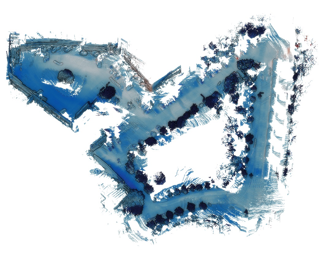
(e) Map 11

(f) Map 14

Figure 6: Result of estimated trajectory and 3D temperature mapping. 6(a)-6(c) the estimated trajectory and VRS-GPS position information. Regions lacking VRS-GPS accuracy are excluded. 6(d)-6(f) the temperature range is colored from 0 to 30 degrees. Note that the night-time temperature is close to $0^{\circ}$, so it represents a dark blue color. We used balance colormap from cmoceans [33].

In general, the output image of a thermal-infrared camera is known to degrade due to spatial non-uniformities induced from fixed-pattern noise [34]. To solve this problem, most thermal cameras provide NUC (NUC) using a mechanical shutter. However, every time the NUC is executed, the camera delays by a few seconds and new incoming data may be lost. This blackout causes fatal defects in motion estimation. Our entire experiment was performed with the NUC disabled. The results show that the effects of fixed-pattern noise are negligible.

The thermal-LiDAR sensor system was mounted on a car-like vehicle (outdoors) or was hand-held (subterranean). For the outdoor experiment, the vehicle was also equipped with a VRS-GPS providing accurate positions ($20\text{\,}\mathrm{m}\mathrm{m}$ in a fixed state and $1\text{\,}\mathrm{m}$ in a floating state). Therefore, we leveraged the measured position at fixed and floating state as the ground truth when computing the estimation error.

V-A Outdoor Experiments

TABLE II: RMSE between the VRS-GPS and estimated positions. The blank (-) indicates failures.

Seq. Number	Traveled distance [m]	Time of day	Proposed [m]	ORB-SLAM [m]
Seq 01 (2019-01-17-16-27-31)	108	day (4pm)	0.698	1.160
Seq 02 (2019-01-17-16-47-37)	996	day (4pm)	4.758	6.693
Seq 03 (2019-01-17-17-15-56)	1031	day (5pm)	5.340	15.553
Seq 04 (2019-01-30-23-28-13)	129	night (11pm)	0.690	-
Seq 05 (2019-01-30-23-30-43)	284	night (11pm)	1.076	-
Seq 06 (2019-01-31-01-09-33)	835	night (1am)	3.586	-
Seq 07 (2019-02-16-13-08-52)	390	day (1pm)	1.521	1.667
Seq 08 (2019-02-16-13-15-27)	383	day (1pm)	1.264	6.821
Seq 09 (2019-02-16-16-41-04)	924	day (4pm)	2.931	6.601
Seq 10 (2019-02-16-16-54-30)	883	day (4pm)	3.519	42.014
Seq 11 (2019-02-16-17-15-36)	604	day (5pm)	1.818	3.108
Seq 12 (2019-02-16-19-53-31)	365	night (7pm)	1.195	-
Seq 13 (2019-02-16-20-02-51)	1003	night (8pm)	6.398	8.830
Seq 14 (2019-02-16-20-16-59)	877	night (8pm)	4.193	7.744

The outdoor experiments were conducted on a campus environment including parking lots, roads, surrounding buildings, and trees. Unlike the RGB image acquired from the visible camera, the thermal camera detects the infrared energy emitted or reflected from the object, not being affected by the light source and applicable regardless of day and night as shown in Fig. 5.

For evaluation, we collected a dataset consisting of 14 sequences. The traversed distance of the dataset is $8.8\text{\,}\mathrm{k}\mathrm{m}$ in total, containing data in the daytime and night-time. In each sequence, we compared the trajectory of the proposed method against ORB-SLAM using the global position provided by the VRS-GPS. Since the ground truth was provided at intervals of $1\text{\,}\mathrm{H}\mathrm{z}$ and the accuracy is sparsely guaranteed only in the fixed and float states, we interpolated and aligned the estimated trajectories based on the timestamp of the VRS-GPS and then calculated the absolute position error with the global position. In addition, since ORB-SLAM utilizes only a thermal-camera, an accurate scale cloud not be obtained. For a fair evaluation, we calculated the absolute position error after compensating the scale to match the trajectory provided by the VRS-GPS with the trajectory of the ORB-SLAM. For ORB-SLAM requiring an 8-bit intensity image in this evaluation, we used an image that rescaled the raw temperature value from $0^{\circ}$ to $30^{\circ}$.

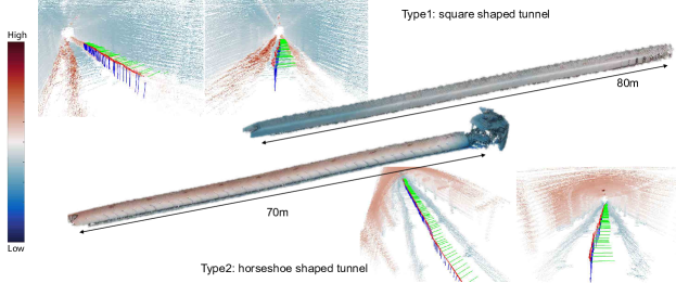
Figure 7: 3D temperature map generated from subterranean tunnels. We performed experiments in two tunnels, a horseshoe type tunnel, and a square type tunnel. The width and height of the two tunnels are 2.5m. The path lengths are 70m and 80m, respectively. Our experiments were carried out by moving the thermal-LiDAR sensor hand-held and walking in the forward direction. The temperature distribution of the two tunnels was quite different. The square type tunnel has colder ceiling while the horseshoe type tunnel overall warmer temperature as can be seen in the local view of each tunnel. The estimated camera coordinates are plotted colored coordinate in the local views. The color code is red for the x-axis, green for the y-axis, and blue for the z-axis.

Fig. 6 depicts trajectory estimation and 3D thermal mapping results in three sequences. The plot was generated excluding GPS-denied regions where VRS-GPS was unavailable to provide a precise global position at the cm-level. Our method is not only globally consistent but also provides a smooth trajectory over all regions. We depicted temperature associated point could simultaneously performing both 3D thermal mapping and the motion estimation.

Table. II shows the absolute position error between the estimated position and ground truth. The proposed method outperformed the ORB-SLAM for the entire sequence. Compared to ORB-SLAM failing at night-time, the proposed method presents consistent performance both in the daytime and night-time. In both methods, the absolute position error tends to increase as the traveled distance increases. This is considered to be due to an accumulation of errors caused by an increase in traveled distance. For the night time missions, Seq 04 to 06, rescaling to 8-bit with a fixed range resulted in a low contrast image and initialization failure for ORB-SLAM. These low contrast images also induced some larger errors in the ORB-SLAM under rotational motion during Seq 03 and 11.

V-B Subterranean Experiments

Secondly, we conducted experiments in two man-made subterranean tunnels, a horseshoe and a square type tunnel. By hand-holding the sensor systems, the data was captured by human working along the tunnel. In particular, the square type tunnel was surveyed in a completely dark environment. Since there is no available ground-truth, we only show the generated 3D temperature map as a qualitative result in Fig. 7.

VI Conclusions

We present a direct thermal-infrared SLAM that utilizes sparse depth from LiDAR. Our approach is to perform motion estimation by directly tracking the sparse depth on a 14-bit raw thermal image. Keyframe-based local refinement improved local accuracy, while loop closure modules enhanced global consistency. The experiment was conducted with a portable thermal-infrared camera and LiDAR. Including daytime and night-time and complete darkness, we achieved an all-day visual SLAM with an accurate trajectory and a 3D thermographic map.

References

- [1] C. Forster, M. Pizzoli, and D. Scaramuzza, “SVO: Fast semi-direct monocular visual odometry,” in Proc. IEEE Intl. Conf. on Robot. and Automat., 2014, pp. 15–22.
- [2] R. Mur-Artal, J. M. M. Montiel, and J. D. Tardós, “ORB-SLAM: A versatile and accurate monocular SLAM system,” IEEE Trans. Robot., vol. 31, no. 5, pp. 1147–1163, 2015.
- [3] J. Zhang, M. Kaess, and S. Singh, “A real-time method for depth enhanced visual odometry,” Autonomous Robots, vol. 41, no. 1, pp. 31–43, 2017.
- [4] T. Mouats, N. Aouf, L. Chermak, and M. A. Richardson, “Thermal stereo odometry for UAVs,” IEEE Sensors J., vol. 15, no. 11, pp. 6335–6347, Nov 2015.
- [5] J. Poujol, C. A. Aguilera, E. Danos, B. X. Vintimilla, R. Toledo, and A. D. Sappa, “A visible-thermal fusion based monocular visual odometry,” in Second Iberian Robotics Conference, 2016, pp. 517–528.
- [6] A. Beauvisage, N. Aouf, and H. Courtois, “Multi-spectral visual odometry for unmanned air vehicles,” in IEEE Sys., Man, and Cybernetics Magn., Oct 2016, pp. 001 994–001 999.
- [7] C. Papachristos, S. Khattak, and K. Alexis, “Autonomous exploration of visually-degraded environments using aerial robots,” in ICUAS, June 2017, pp. 775–780.
- [8] L. Chen, L. Sun, T. Yang, L. Fan, K. Huang, and Z. Xuanyuan, “RGB-T SLAM: A flexible SLAM framework by combining appearance and thermal information,” in Proc. IEEE Intl. Conf. on Robot. and Automat., May 2017, pp. 5682–5687.
- [9] C. Kerl, J. Sturm, and D. Cremers, “Robust odometry estimation for RGB-D cameras,” in Proc. IEEE Intl. Conf. on Robot. and Automat., 2013, pp. 3748–3754.
- [10] J. Engel, V. Koltun, and D. Cremers, “Direct sparse odometry,” IEEE Trans. Pattern Analysis and Machine Intell., vol. PP, no. 99, pp. 1–1, 2017.
- [11] I. Cvišić, J. Ćesić, I. Marković, and I. Petrović, “SOFT-SLAM: Computationally efficient stereo visual simultaneous localization and mapping for autonomous unmanned aerial vehicles,” J. of Field Robot., vol. 35, no. 4, pp. 578–595, 2018.
- [12] J. Engel, T. Schöps, and D. Cremers, “LSD-SLAM: Large-scale direct monocular SLAM,” in Proc. European Conf. on Comput. Vision, 2014.
- [13] P. Kim, B. Coltin, O. Alexandrov, and H. J. Kim, “Robust visual localization in changing lighting conditions,” in Proc. IEEE Intl. Conf. on Robot. and Automat., May 2017, pp. 5447–5452.
- [14] G. Bitelli, P. Conte, T. Csoknyai, F. Franci, V. A. Girelli, and E. Mandanici, “Aerial thermography for energetic modelling of cities,” Remote Sensing, vol. 7, no. 2, pp. 2152–2170, 2015.
- [15] E. Mandanici, P. Conte, and V. A. Girelli, “Integration of aerial thermal imagery, LiDAR data and ground surveys for surface temperature mapping in urban environments,” Remote Sensing, vol. 8, p. 880, 2016.
- [16] D. González-Aguilera, P. Rodriguez-Gonzalvez, J. Armesto, and S. Lagüela, “Novel approach to 3D thermography and energy efficiency evaluation,” Energy and Buildings, vol. 54, pp. 436 – 443, 2012.
- [17] R. A. Newcombe, S. Izadi, O. Hilliges, D. Molyneaux, D. Kim, A. J. Davison, P. Kohi, J. Shotton, S. Hodges, and A. Fitzgibbon, “KinectFusion: Real-time dense surface mapping and tracking,” in Proc. Intl. Symp. on Mixed and Aug. Reality, 2011, pp. 127–136.
- [18] T. Whelan, M. Kaess, H. Johannsson, M. Fallon, J. J. Leonard, and J. McDonald, “Real-time large-scale dense RGB-D slam with volumetric fusion,” Intl. J. of Robot. Research, vol. 34, no. 4-5, pp. 598–626, 2015.
- [19] S. Vidas, P. Moghadam, and M. Bosse, “3D thermal mapping of building interiors using an RGB-D and thermal camera,” in Proc. IEEE Intl. Conf. on Robot. and Automat., May 2013, pp. 2311–2318.
- [20] S. Vidas and P. Moghadam, “HeatWave: A handheld 3D thermography system for energy auditing,” Energy and Buildings, vol. 66, pp. 445 – 460, 2013.
- [21] S. Zhao, Z. Fang, and S. Wen, “A real-time handheld 3D temperature field reconstruction system,” in IEEE Trans. Cybernetics, July 2017, pp. 289–294.
- [22] Y. Cao, B. Xu, Z. Ye, J. Yang, Y. Cao, C.-L. Tisse, and X. Li, “Depth and thermal sensor fusion to enhance 3D thermographic reconstruction,” Opt. Express, vol. 26, no. 7, pp. 8179–8193, Apr 2018.
- [23] Y.-S. Shin, Y. S. Park, and A. Kim, “Direct visual SLAM using sparse depth for camera-lidar system,” in Proc. IEEE Intl. Conf. on Robot. and Automat., Brisbane, May. 2018, pp. 1–8.
- [24] A. Geiger, F. Moosmann, O. Car, and B. Schuster, “Automatic camera and range sensor calibration using a single shot,” in Proc. IEEE Intl. Conf. on Robot. and Automat., May 2012, pp. 3936–3943.
- [25] A. Kassir and T. Peynot, “Reliable automatic camera-laser calibration,” G. Wyeth and B. Upcroft, Eds., Brisbane, Queensland, December 2010.
- [26] Q. Zhang and R. Pless, “Extrinsic calibration of a camera and laser range finder (improves camera calibration),” in Proc. IEEE/RSJ Intl. Conf. on Intell. Robots and Sys., Sep. 2004, pp. 2301–2306.
- [27] J. T. Lussier and S. Thrun, “Automatic calibration of RGBD and thermal cameras,” in Proc. IEEE/RSJ Intl. Conf. on Intell. Robots and Sys., Sep. 2014, pp. 451–458.
- [28] Y. Choi, N. Kim, S. Hwang, K. Park, J. S. Yoon, K. An, and I. S. Kweon, “KAIST multi-spectral day/night data set for autonomous and assisted driving,” IEEE Trans. Intell. Transport. Sys., vol. 19, no. 3, pp. 934–948, March 2018.
- [29] R. Hartley and A. Zisserman, Multiple view geometry in computer vision. Cambridge university press, 2003.
- [30] D. Gálvez-López and J. D. Tardós, “Bags of binary words for fast place recognition in image sequences,” IEEE Trans. Robot., vol. 28, no. 5, pp. 1188–1197, 2012.
- [31] H. Jin, P. Favaro, and S. Soatto, “Real-time feature tracking and outlier rejection with changes in illumination,” in Proc. IEEE Intl. Conf. on Comput. Vision, vol. 1, July 2001, pp. 684–689 vol.1.
- [32] J. Engel, J. Stückler, and D. Cremers, “Large-scale direct SLAM with stereo cameras,” in Proc. IEEE/RSJ Intl. Conf. on Intell. Robots and Sys., Sep. 2015, pp. 1935–1942.
- [33] K. Thyng, C. Greene, R. Hetland, H. Zimmerle, and S. DiMarco, “True colors of oceanography,” Oceanography, vol. 29, no. 3, 2016.
- [34] S. K. Sobarzo and S. N. Torres, “Real-time Kalman filtering for nonuniformity correction on infrared image sequences: Performance and analysis,” in Prog. in Patt. Recog., Img. Anal. and App., A. Sanfeliu and M. L. Cortés, Eds., 2005, pp. 752–761.