Deep Interpretable Non-Rigid Structure from Motion

Abstract

All current non-rigid structure from motion (NRSfM) algorithms are limited with respect to: (i) the number of images, and (ii) the type of shape variability they can handle. This has hampered the practical utility of NRSfM for many applications within vision. In this paper we propose a novel deep neural network to recover camera poses and 3D points solely from an ensemble of 2D image coordinates. The proposed neural network is mathematically interpretable as a multi-layer block sparse dictionary learning problem, and can handle problems of unprecedented scale and shape complexity. Extensive experiments demonstrate the impressive performance of our approach where we exhibit superior precision and robustness against all available state-of-the-art works. The considerable model capacity of our approach affords remarkable generalization to unseen data. We propose a quality measure (based on the network weights) which circumvents the need for 3D ground-truth to ascertain the confidence we have in the reconstruction. Once the network’s weights are estimated (for a non-rigid object) we show how our approach can effectively recover 3D shape from a single image – outperforming comparable methods that rely on direct 3D supervision.

1 Introduction

Building an AI capable of inferring the 3D structure and pose of an object from a single image is a problem of immense importance. Training such a system using supervised learning requires a large number of labeled images – how to obtain these labels is currently an open problem for the vision community. Rendering [33] is problematic as the synthetic images seldom match the appearance and geometry of the objects we encounter in the real-world. Hand annotation is preferable, but current strategies rely on associating the natural images with an external 3D dataset (e.g. ShapeNet [5], ModelNet [39]), which we refer to as 3D supervision. If the 3D shape dataset does not capture the variation we see in the imagery, then the problem is inherently ill-posed.

(a) Non-rigid object: moving person.

(b) Object category: chair.

Figure 1: Randomly selected 3D reconstructions by our deep NRSfM method based on multi-layer sparse coding model. Spheres in (a) and red cubes in (b) are reconstructed points. Bars, planes are manually added for visualization.

Non-Rigid Structure from Motion (NRSfM) offers computer vision a way out of this quandary – by recovering the pose and 3D structure of an object category solely from hand annotated 2D landmarks with no need of 3D supervision. Classically [3], the problem of NRSfM has been applied to objects that move non-rigidly over time such as the human body and face. But NRSfM is not restricted to non-rigid objects; it can equally be applied to rigid objects whose object categories deform non-rigidly [20]. Consider, for example, the four objects in Figure 1 (b), our reconstructions from the visual object category “chair”. Each object in isolation represents a rigid chair, but the set of all 3D shapes describing “chair” is non-rigid. In other words, each object instance can be modeled as a deformation from its category’s general shape.

Current NRSfM algorithms [21, 23, 7] all suffer from the difficulty of processing large-scale image sequences, limiting their ability to reliably model complex shape variations. This additionally hinders their ability to generalize to unseen images. Deep Neural Networks (DNNs) are an obvious candidate to help with such issue. However, the influence of DNNs has been most noticeable when applied to raster representations (e.g. raw pixel intensities [11]). While DNNs have recently exhibited their success to 3D point representations (e.g. point clouds) [30, 18], their use has not been explored in recovering poses and 3D shapes from an ensemble of vector-based 2D landmarks.

1.0.1 Contributions

We propose a novel DNN to solve the problem of NRSfM. Our employment of DNNs moves from an opaque black-box to a transparent “glass-box” in terms of its interpretability. The term “black-box” is often used as a critique of DNNs with respect to the general lack of understanding surrounding the inner workings. We demonstrate how the problem of NRSfM can be cast as a multi-layer block sparse dictionary learning problem. Through recent theoretical innovations [29], we then show how this problem can be reinterpreted as a feed-forward DNN auto-encoder that can be efficiently solved through modern deep learning environments.

Our deep NRSfM is capable of handling hundreds of thousands of images and learning large parameterizations to model non-rigidity. Our proposed approach is completely unsupervised in a 3D sense, relying solely on the projected 2D landmarks of the non-rigid object or object category to recover the pose and 3D shape. Our approach dramatically outperforms state-of-the-art methods on a number of benchmarks, and gets impressive qualitative reconstructions on the problem of NRSfM – examples of which are shown in Figure 1. Moreover, the considerable capacity of modeling non-rigidity allows us to efficiently apply it to unseen data. This facilitates an accurate 3D reconstruction of objects from a single view with no aid of 3D ground-truth. Finally, we propose a measure of model quality (using coherence and trained parameters), which improves the practical utility of our model in the real world applications.

2 Related Work

2.0.1 Non-rigid structure from motion

NRSfM is an inherently ill-posed problem since the 3D shapes can vary between images, resulting in more variables than equations. To alleviate the ill-posedness, various constraints are exploited including temporal  [1, 14, 22, 21], and articulation [31] priors. Dai et al. [8] pioneered the exploration of NRSfM with minimum assumptions. They proposed a low-rank model of non-rigidity and a factorization algorithm recovering both cameras and 3D shapes with no need of additional priors. The major drawback of this method is the low rank assumption, which highly restricts the application to complex sequences. To solve this problem, Kong and Lucey [19] proposed to use an over-complete dictionary with sparsity to model non-rigid objects and upgraded the factorization algorithm by characterizing the uniqueness of dictionary learning. However, due to the enormous parameter space, their method was sensitive to noise and thus had limited utility in real world applications.

2.0.2 Structure from category

NRSfM has often been criticized as solving a toy problem with few useful applications beyond being a theoretical curiosity for computer vision. Recently, Kong et al. [20] proposed a novel concept—Structure from Category (SfC)—directly connecting NRSfM to inferring camera poses and 3D structure within an ensemble of images stemming from the same object category. The strength of this approach is the ability to solely use 2D landmarks without 3D supervision. They provided a convex relaxation solution to this problem. However, the proposed optimization algorithm could not be applied to large-scale images, limiting its effectiveness for modeling complex shape variations.

2.0.3 Single view human pose estimation

Besides SfC and NRSfM, there is another task related to our work, that is single view human pose estimation. A common solution is assuming that the human body can be represented through a sparse dictionary. Ramakrishna et al. [31] proposed to use a matching pursuit algorithm to estimate the sparse representation. However, since the problem is not convex, their algorithm fails when initialization is poor. Zhou et al. [40] proposed to utilize a convex relaxation to alleviate sensitivities to initialization, but inevitably introduce additional errors. Another drawback from Zhou et al. [40, 31] is its dependence on external 3D models for estimating the model dictionary (i.e. 3D supervision).

3 Background

Sparse dictionary learning can be considered as an unsupervised learning task and divided into two sub-problems: (i) dictionary learning, and (ii) sparse code recovery. Let us consider sparse code recovery problem, where we estimate a sparse representation $\mathbf{z}$ for a measurement vector $\mathbf{x}$ given the dictionary $\mathbf{W}$ i.e.

$$\min_{\mathbf{z}}\|\mathbf{x}-\mathbf{W}\mathbf{z}\|_{2}^{2}\quad\ \mathrm{s.t.}\ \|\mathbf{z}\|_{0}<\lambda,$$ (1)

where $\lambda$ related to the trust region controls the sparsity of recovered code. One classical algorithm to recover the sparse representation is Iterative Shrinkage and Thresholding Algorithm (ISTA) [9, 32, 2]. ISTA iteratively executes the following two steps with $\mathbf{z}^{[0]}=\mathbf{0}$:

$$\mathbf{v}=\mathbf{z}^{[i]}-\alpha\mathbf{W}^{T}(\mathbf{W}\mathbf{z}^{[i]}-\mathbf{x}),$$ (2)

$$\mathbf{z}^{[i+1]}=\operatorname*{argmin}_{\mathbf{u}}\frac{1}{2}\|\mathbf{u}-\mathbf{v}\|^{2}_{2}+\tau\|\mathbf{u}\|_{1},$$ (3)

which first uses the gradient of $\|\mathbf{x}-\mathbf{W}\mathbf{z}\|_{2}^{2}$ to update $\mathbf{z}^{[i]}$ in step size $\alpha$ and then finds the closest sparse solution using an $\ell_{1}$ convex relaxation. It is well known in literature that the second step has a closed-form solution using soft thresholding operator. Therefore, ISTA can be summarized as the following recursive equation:

$$\mathbf{z}^{[i+1]}=h_{\tau}\big{(}\mathbf{z}^{[i]}-\alpha\mathbf{W}^{T}(\mathbf{W}\mathbf{z}^{[i]}-\mathbf{x})\big{)},$$ (4)

where $h_{\tau}$ is a soft thresholding operator and $\tau$ is related to $\lambda$ for controlling sparsity.

Recently, Papyan [29] proposed to use ISTA and sparse coding to reinterpret feed-forward neural networks. They argue that feed-forward passing a single-layer neural network $\mathbf{z}=\mathop{\mathrm{ReLU}}(\mathbf{W}^{T}\mathbf{x}-b)$ can be considered as one iteration of ISTA when $\mathbf{z}~{}\geq~{}0,\alpha=1$ and $\tau=b$. Based on this insight, the authors extend this interpretation to feed-forward neural network with $n$ layers

$$\mathbf{z}_{1} =\mathop{\mathrm{ReLU}}(\mathbf{W}_{1}^{T}\mathbf{x}-b_{1})$$ (5)

$$\mathbf{z}_{2} =\mathop{\mathrm{ReLU}}(\mathbf{W}_{2}^{T}\mathbf{z}_{1}-b_{2})$$

$$\quad\vdots$$

$$\mathbf{z}_{n} =\mathop{\mathrm{ReLU}}(\mathbf{W}_{n}^{T}\mathbf{z}_{n-1}-b_{n})$$

as executing a sequence of single-iteration ISTA, serving as an approximate solution to the multi-layer sparse coding problem: find $\{\mathbf{z}_{i}\}_{i=1}^{n}$, such that

$$\mathbf{x}=\mathbf{W}_{1}\mathbf{z}_{1} ,\quad\|\mathbf{z}_{1}\|_{0}<\lambda_{1},\mathbf{z}_{1}\geq 0,$$ (6)

$$\mathbf{z}_{1}=\mathbf{W}_{2}\mathbf{z}_{2} ,\quad\|\mathbf{z}_{2}\|_{0}<\lambda_{2},\mathbf{z}_{2}\geq 0,$$

$$\vdots ,\quad\quad\vdots$$

$$\mathbf{z}_{n-1}=\mathbf{W}_{n}\mathbf{z}_{n} ,\quad\|\mathbf{z}_{n}\|_{0}<\lambda_{n},\mathbf{z}_{n}\geq 0,$$

where the bias terms $\{b_{i}\}_{i=1}^{n}$ (in a similar manner to $\tau$) are related to $\{\lambda_{i}\}_{i=1}^{n}$, adjusting the sparsity of recovered code. Furthermore, they reinterpret back-propagating through the deep neural network as learning the dictionaries $\{\mathbf{W}_{i}\}_{i=1}^{n}$. This connection offers a novel breakthrough for understanding DNNs. In this paper, we extend this to the block sparse scenario and apply it to solving our NRSfM problem.

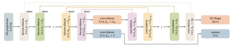
Figure 2: Deep NRSfM architecture. The network can be divided into two parts: encoder and decoder that are symmetric and share convolution kernels (i.e. dictionaries). The symbol $a\times b,c\to d$ refers to the operator using kernel size $a\times b$ with $c$ input channels and $d$ output channels.

4 Deep Non-Rigid Structure from Motion

Under weak-perspective projection, NRSfM deals with the problem of factorizing a 2D projection matrix $\mathbf{W}\in\mathbb{R}^{p\times 2}$ as the product of a 3D shape matrix $\mathbf{S}\in\mathbb{R}^{p\times 3}$ and camera matrix $\mathbf{M}\in\mathbb{R}^{3\times 2}$. Formally,

$$\mathbf{W}=\mathbf{S}\mathbf{M},$$ (7)

$$\mathbf{W}=\begin{bmatrix}u_{1}&v_{1}\\ u_{2}&v_{2}\\ \vdots&\vdots\\ u_{p}&v_{p}\end{bmatrix},~{}\mathbf{S}=\begin{bmatrix}x_{1}&y_{1}&z_{1}\\ x_{2}&y_{2}&z_{2}\\ \vdots&\vdots&\vdots\\ x_{p}&y_{p}&z_{p}\end{bmatrix},~{}\mathbf{M}^{T}\mathbf{M}=\mathbf{I}_{2},$$ (8)

where $(u_{i},v_{i}),(x_{i},y_{i},z_{i})$ are the image and world coordinates of the $i$-th point. Due to the scale ambiguity between camera focal length and shape size, we ignore camera scale. The goal of NRSfM is to recover simultaneously the shape $\mathbf{S}$ and the camera $\mathbf{M}$ for each projection $\mathbf{W}$ in a given set $\mathbb{W}$ of 2D landmarks. In a general NRSfM including SfC, this set $\mathbb{W}$ could contain deformations of a non-rigid object or various instances from an object category.

4.1 Modeling via multi-layer sparse coding

To alleviate the ill-posedness of NRSfM and also guarantee sufficient freedom on shape variation, we propose a novel prior assumption on 3D shapes via multi-layer sparse coding: The vectorization of $\mathbf{S}$ satisfies

$$\mathbf{s}=\mathbf{D}_{1}\boldsymbol{\psi}_{1} ,\quad\|\boldsymbol{\psi}_{1}\|_{0}<\lambda_{1},\boldsymbol{\psi}_{1}\geq 0,$$ (9)

$$\boldsymbol{\psi}_{1}=\mathbf{D}_{2}\boldsymbol{\psi}_{2} ,\quad\|\boldsymbol{\psi}_{2}\|_{0}<\lambda_{2},\boldsymbol{\psi}_{2}\geq 0,$$

$$\vdots ,\quad\quad\vdots$$

$$\boldsymbol{\psi}_{n-1}=\mathbf{D}_{n}\boldsymbol{\psi}_{n} ,\quad\|\boldsymbol{\psi}_{n}\|_{0}<\lambda_{n},\boldsymbol{\psi}_{n}\geq 0,$$

where $\mathbf{D}_{1}\in\mathbb{R}^{3p\times k_{1}},\mathbf{D}_{2}\in\mathbb{R}^{k_{1}\times k_{2}},\dots,\mathbf{D}_{n}\in\mathbb{R}^{k_{n-1}\times k_{n}}$ are hierarchical dictionaries. In this prior, each non-rigid shape is represented by a sequence of hierarchical dictionaries and corresponding sparse codes. Each sparse code is determined by its lower-level neighbor and affects the next-level. Clearly this hierarchy adds more parameters, and thus more freedom into the system. We now show that it paradoxically results in a more constrained global dictionary and sparse code recovery.

4.1.1 More constrained code recovery

In a classical single dictionary system, the constraint on the representation is element-wise sparsity. Further, the quality of its recovery entirely depends on the quality of the dictionary. In our multi-layer sparse coding model, the optimal code not only minimizes the difference between measurements $\mathbf{s}$ and $\mathbf{D}_{1}\boldsymbol{\psi}_{1}$ along with sparsity regularization $\|\boldsymbol{\psi}_{1}\|_{0}$, but also satisfies constraints from its subsequent representations. This additional joint inference imposes more constraints on code recovery, helps to control the uniqueness and therefore alleviates its heavy dependency on the dictionary quality.

4.1.2 More constrained dictionary

When all equality constraints are satisfied, the multi-layer sparse coding model degenerates to a single dictionary system. From Equation 9, by denoting $\mathbf{D}^{(l)}=\prod_{i=1}^{l}\mathbf{D}_{i}$, it is implied that $\mathbf{s}=\mathbf{D}_{1}\mathbf{D}_{2}\dots\mathbf{D}_{n}\boldsymbol{\psi}_{n}=\mathbf{D}^{(n)}\boldsymbol{\psi}_{n}$. However, this differs from other single dictionary models [41, 42, 19, 20, 40] in terms that a unique structure is imposed on $\mathbf{D}^{(n)}$ [34]. The dictionary $\mathbf{D}^{(n)}$ is composed by simpler atoms hierarchically. For example, each column of $\mathbf{D}^{(2)}=\mathbf{D}_{1}\mathbf{D}_{2}$ is a linear combination of atoms in $\mathbf{D}_{1}$, each column of $\mathbf{D}^{(3)}=\mathbf{D}^{(2)}\mathbf{D}_{3}$ is a linear combination of atoms in $\mathbf{D}^{(2)}$ and so on. Such a structure results in a more constrained global dictionary and potentially leads to higher quality with lower mutual coherence [13].

4.2 Multi-layer block sparse coding

Given the proposed multi-layer sparse coding model, we now build a conduit from the proposed shape code $\{\boldsymbol{\psi}_{i}\}_{i=1}^{k}$ to the 2D projected points. From Equation 9, we reshape vector $\mathbf{s}$ to a matrix $\mathbf{S}\in\mathbb{R}^{p\times 3}$ such that $\mathbf{S}=\mathbf{D}^{\sharp}_{1}(\boldsymbol{\psi}_{1}\otimes\mathbf{I}_{3})$, where $\otimes$ is Kronecker product and $\mathbf{D}_{1}^{\sharp}\in\mathbb{R}^{p\times 3k_{1}}$ is a reshape of $\mathbf{D}_{1}$ [8]. From linear algebra, it is well known that $\mathbf{A}\mathbf{B}\otimes\mathbf{I}=(\mathbf{A}\otimes\mathbf{I})(\mathbf{B}\otimes\mathbf{I})$ given three matrices $\mathbf{A},\mathbf{B}$, and identity matrix $\mathbf{I}$. Based on this lemma, we can derive that

$$\mathbf{S}=\mathbf{D}^{\sharp}_{1}(\boldsymbol{\psi}_{1}\otimes\mathbf{I}_{3}) ,\quad\|\boldsymbol{\psi}_{1}\|_{0}<\lambda_{1},\boldsymbol{\psi}_{1}\geq 0,$$ (10)

$$\boldsymbol{\psi}_{1}\otimes\mathbf{I}_{3}=(\mathbf{D}_{2}\otimes\mathbf{I}_{3})(\boldsymbol{\psi}_{2}\otimes\mathbf{I}_{3}) ,\quad\|\boldsymbol{\psi}_{2}\|_{0}<\lambda_{2},\boldsymbol{\psi}_{2}\geq 0,$$

$$\vdots ,\quad\quad\vdots$$

$$\boldsymbol{\psi}_{n-1}\otimes\mathbf{I}_{3}=(\mathbf{D}_{n}\otimes\mathbf{I}_{3})(\boldsymbol{\psi}_{n}\otimes\mathbf{I}_{3}) ,\quad\|\boldsymbol{\psi}_{n}\|_{0}<\lambda_{n},\boldsymbol{\psi}_{n}\geq 0.$$

Further, from Equation 7, by right multiplying the camera matrix $\mathbf{M}\in\mathbb{R}^{3\times 2}$ to the both sides of Equation 10 and denote $\boldsymbol{\Psi}_{i}=\boldsymbol{\psi}_{i}\otimes\mathbf{M}$, we obtain that

$$\mathbf{W}=\mathbf{D}^{\sharp}_{1}\boldsymbol{\Psi}_{1} ,\quad\|\boldsymbol{\Psi}_{1}\|_{0}^{(3\times 2)}<\lambda_{1},$$ (11)

$$\boldsymbol{\Psi}_{1}=(\mathbf{D}_{2}\otimes\mathbf{I}_{3})\boldsymbol{\Psi}_{2} ,\quad\|\boldsymbol{\Psi}_{2}\|_{0}^{(3\times 2)}<\lambda_{2},$$

$$\vdots ,\quad\quad\vdots$$

$$\boldsymbol{\Psi}_{n-1}=(\mathbf{D}_{n}\otimes\mathbf{I}_{3})\boldsymbol{\Psi}_{n} ,\quad\|\boldsymbol{\Psi}_{n}\|_{0}^{(3\times 2)}<\lambda_{n},$$

where $\|\cdot\|_{0}^{(3\times 2)}$ divides the argument matrix into blocks with size $3\times 2$ and counts the number of active blocks. Since $\boldsymbol{\psi}_{i}$ has active elements less than $\lambda_{i}$, $\boldsymbol{\Psi}_{i}$ has active blocks less than $\lambda_{i}$, that is $\boldsymbol{\Psi}_{i}$ is block sparse. This derivation demonstrates that if the shape vector $\mathbf{s}$ satisfies the multi-layer sparse coding prior described by Equation 9, then its 2D projection $\mathbf{W}$ must be in the format of multi-layer block sparse coding described by Equation 11. We hereby interpret NRSfM as a hierarchical block sparse dictionary learning problem i.e. factorizing $\mathbf{W}$ as products of hierarchical dictionaries $\{\mathbf{D}_{i}\}_{i=1}^{n}$ and block sparse coefficients $\{\boldsymbol{\Psi}_{i}\}_{i=1}^{n}$.

4.3 Block ISTA and DNNs solution

Before solving the multi-layer block sparse coding problem in Equation 11, we first consider the single-layer problem:

$$\min_{\mathbf{Z}}\|\mathbf{X}-\mathbf{W}\mathbf{Z}\|_{F}^{2}\quad\ \mathrm{s.t.}\ ~{}\|\mathbf{Z}\|_{0}^{(3\times 2)}<\lambda.$$ (12)

Inspired by ISTA, we propose to solve this problem by iteratively executing the following two steps:

$$\mathbf{V}=\mathbf{Z}^{[i]}-\alpha\mathbf{W}^{T}(\mathbf{W}\mathbf{Z}^{[i]}-\mathbf{X}),$$ (13)

$$\mathbf{Z}^{[i+1]}=\operatorname*{argmin}_{\mathbf{U}}\frac{1}{2}\|\mathbf{U}-\mathbf{V}\|^{2}_{F}+\tau\|\mathbf{U}\|_{F1}^{(3\times 2)},$$ (14)

where $\|\cdot\|_{F1}^{(3\times 2)}$ is defined as the summation of Frobenius norm of each $3\times 2$ block, serving as a convex relaxation of block sparsity constraint. It is derived in [12] that the second step has a closed-form solution computing each block separately by $\small\mathbf{Z}^{[i+1]}_{j}=(h_{\tau}(\|\mathbf{V}_{j}\|_{F})/\|\mathbf{V}_{j}\|_{F})\mathbf{V}_{j}$, where the subscript $j$ represents the $j$-th block and $h_{\tau}$ is a soft thresholding operator. However, soft thresholding the Frobenius norms for every block brings unnecessary computational complexity. We show in the supplementary material that an efficient relaxation is $\mathbf{Z}^{[i+1]}_{j}=h_{b_{j}}(\mathbf{V}_{j})$, where $b_{j}$ is the threshold for the $j$-th block, controlling its sparsity. Based on this relaxation, a single-iteration block ISTA with step size $\alpha=1$ can be represented by :

$$\mathbf{Z}=h_{\mathbf{b}}\big{(}\mathbf{W}^{T}\mathbf{X}\big{)}=\mathop{\mathrm{ReLU}}(\mathbf{W}^{T}\mathbf{X}-\mathbf{b}\otimes\mathbf{1}_{3\times 2}),$$ (15)

where $h_{\mathbf{b}}$ is a soft thresholding operator using the $j$-th element $b_{j}$ as threshold of the $j$-th block and the second equality holds if $\mathbf{Z}$ is non-negative.

4.3.1 Encoder

Recall from Section 3 that the feed-forward pass through a deep neural network can be considered as a sequence of single ISTA iterations and thus provides an approximate recovery of multi-layer sparse codes. We follow the same scheme: we first relax the multi-layer block sparse coding to be non-negative and then sequentially use single-iteration block ISTA to solve it i.e.

$$\boldsymbol{\Psi}_{1} =\mathop{\mathrm{ReLU}}((\mathbf{D}^{\sharp}_{1})^{T}\mathbf{W}-\mathbf{b}_{1}\otimes\mathbf{1}_{3\times 2}),$$ (16)

$$\boldsymbol{\Psi}_{2} =\mathop{\mathrm{ReLU}}((\mathbf{D}_{2}\otimes\mathbf{I}_{3})^{T}\boldsymbol{\Psi}_{1}-\mathbf{b}_{2}\otimes\mathbf{1}_{3\times 2}),$$

$$\quad\vdots$$

$$\boldsymbol{\Psi}_{n} =\mathop{\mathrm{ReLU}}((\mathbf{D}_{n}\otimes\mathbf{I}_{3})^{T}\boldsymbol{\Psi}_{n-1}-\mathbf{b}_{n}\otimes\mathbf{1}_{3\times 2}),$$

where thresholds $\mathbf{b}_{1},...,\mathbf{b}_{n}$ are learned, controlling the block sparsity. This learning is crucial because in previous NRSfM algorithms utilizing low-rank [8], subspaces [41] or compressible [19] priors, the weight given to this prior (e.g. rank or sparsity) is hand-selected through a cumbersome cross validation process. In our approach, this weighting is learned simultaneously with all other parameters removing the need for any irksome cross validation process. This formula composes the encoder of our proposed DNN.

4.3.2 Decoder

Let us for now assume that we can extract camera $\mathbf{M}$ and regular sparse hidden code $\boldsymbol{\psi}_{n}$ from $\boldsymbol{\Psi}_{n}$ by some functions i.e. $\mathbf{M}=\mathcal{F}(\boldsymbol{\Psi}_{n})$ and $\boldsymbol{\psi}_{n}=\mathcal{G}(\boldsymbol{\Psi}_{n})$, which will be discussed in the next section. Then we can compute the 3D shape vector $\mathbf{s}$ by:

$$\boldsymbol{\psi}_{n-1} =\mathop{\mathrm{ReLU}}(\mathbf{D}_{n}\boldsymbol{\psi}_{n}-\mathbf{b}_{n}^{\prime}),$$ (17)

$$\quad\vdots$$

$$\boldsymbol{\psi}_{1} =\mathop{\mathrm{ReLU}}(\mathbf{D}_{2}\boldsymbol{\psi}_{2}-\mathbf{b}_{2}^{\prime}),$$

$$\mathbf{s} =\mathbf{D}^{\sharp}_{1}\boldsymbol{\psi}_{1},$$

Note we preserve the ReLU and bias term during decoding to further enforce sparsity and improve robustness. These portion forms the decoder of our DNN.

4.3.3 Variation of implementation

The Kronecker product of identity matrix $\mathbf{I}_{3}$ dramatically increases the time and space complexity of our approach. To eliminate it and make parameter sharing easier in modern deep learning environments (e.g. TensorFlow, PyTorch), we reshape the filters and features and show that the matrix multiplication in each step of the encoder and decoder can be equivalently computed via multi-channel $1\times 1$ convolution ($*$) and transposed convolution ($*^{T}$) i.e.

$$(\mathbf{D}_{1}^{\sharp})^{T}\mathbf{W}=\mathsf{d}_{1}^{\sharp}*^{T}\mathsf{w},$$ (18)

where $\mathsf{d}_{1}^{\sharp}\in\mathbb{R}^{3\times 1\times k_{1}\times p},\mathsf{w}\in\mathbb{R}^{1\times 2\times p}$.

$$(\mathbf{D}_{i+1}\otimes\mathbf{I}_{3})^{T}\boldsymbol{\Psi}_{i}=\mathsf{d}_{i+1}*^{T}\Psi_{i},$$ (19)

where $\mathsf{d}_{i+1}\in\mathbb{R}^{1\times 1\times k_{i+1}\times k_{i}},\Psi_{i}\in\mathbb{R}^{3\times 2\times k_{i}}.$

$$\mathbf{D}_{i}\boldsymbol{\psi}_{i}=\mathsf{d}_{i}*\psi_{i},$$ (20)

where $\mathsf{d}_{i}\in\mathbb{R}^{1\times 1\times k_{i}\times k_{i-1}},\psi_{i}\in\mathbb{R}^{1\times 1\times k_{i}}.$

4.3.4 Code and camera recovery

Estimating $\boldsymbol{\psi}_{n}$ and $\mathbf{M}$ from $\boldsymbol{\Psi}_{n}$ is discussed in [19] and solved by a closed-form formula. Due to its differentiability, we could insert the solution directly within our pipeline. An alternative solution is using a relaxation i.e. a fully connected layer connecting $\boldsymbol{\Psi}_{n}$ and $\boldsymbol{\psi}_{n}$ and a linear combination among each blocks of $\boldsymbol{\Psi}_{n}$ to estimate $\mathbf{M}$, where the fully connected layer parameters and combination coefficients are learned from data. In our experiments, we use the relaxed solution and represent them via convolutions, as shown in Figure 2, for conciseness and maintaining proper dimensions. Since the relaxation has no way to force the orthonormal constraint on the camera, we seek help from the loss function.

	Subject	1	5	18	23	64	70	102	106	123	127
	# of frames	45025	13773	10024	10821	11621	10788	5929	12335	10788	9502
	EM-SfM [36]	110.23%	119.97%	111.05%	110.94%	114.04%	127.11%	111.60%	113.81%	107.67%	108.07%
	Simple [8]	16.45%	14.07%	13.85%	20.03%	18.13%	18.91%	18.78%	18.63%	19.32%	23.70%
	Sparse [19]	71.23%	66.30%	46.72%	52.44%	70.83%	39.42%	74.12%	47.00%	44.46%	73.85%
Shape Error (%)	Ours	10.74%	13.40%	4.73%	3.24%	4.38%	2.17%	7.32%	6.83%	2.23%	6.00%
	EM-SfM [36]	53.1818	60.5971	53.0413	52.2671	50.3960	56.3713	48.5891	50.3306	47.7355	50.8183
	Simple [8]	7.9905	6.9406	6.6340	9.5139	8.1784	8.4294	8.0171	8.1782	8.6922	10.9473
	Sparse [19]	35.0283	35.3014	22.6930	25.3302	32.4681	17.7433	30.8274	21.2735	20.3565	32.4896
Point Error (cm)	Ours	5.0638	6.6717	2.2664	1.5138	2.2909	0.9622	3.0240	2.9130	0.9844	2.6820

Table 1: Quantitative comparison of our method against the state-of-the-art methods in NRSfM task. Human skeletons are scaled to real-world sizes, around 1.8 meters high, and the mean point distance is measured in centimeters.

4.3.5 Loss function

The loss function must measure the reprojection error between input 2D points $\mathbf{W}$ and reprojected 2D points $\mathbf{S}\mathbf{M}$ while simultaneously encouraging orthonormality of the estimated camera $\mathbf{M}$. One solution is to use spectral norm regularization of $\mathbf{M}$ because spectral norm minimization is the tightest convex relaxation of the orthonormal constraint [40]. An alternative solution is to hard code the singular values of $\mathbf{M}$ to be exact ones with the help of Singular Value Decomposition (SVD). Even though SVD is generally non-differentiable, the numeric computation of SVD is differentiable and most deep learning packages implement its gradients (e.g. PyTorch, TensorFlow). In our implementation and experiments, we use SVD to ensure the success of the orthonormal constraint and a simple Frobenius norm to measure reprojection error,

$$Loss=\|\mathbf{W}-\mathbf{S}\tilde{\mathbf{M}}\|_{F},\quad\tilde{\mathbf{M}}=\mathbf{U}\mathbf{V}^{T},$$ (21)

where $\mathbf{U}\boldsymbol{\Sigma}\mathbf{V}^{T}=\mathbf{M}$ is the SVD of the camera matrix.

5 Experiments

We conduct extensive experiments to evaluate the performance of our deep solution for solving NRSfM and SfC problems. Further, for evaluating generalizability, we conduct an experiment applying the pre-trained DNN to unseen data and reconstruct 3D human pose from a single view. Note that in all experiments, our model has no access to 3D ground-truth except qualitative and quantitative evaluations for comparison against the state-of-art methods. A detailed description of our architectures is in the supplementary material.

5.1 NRSfM on CMU Motion Capture

We first apply our method to solving the problem of NRSfM using the CMU motion capture dataset. For evaluation on complex sequences, we concatenate all motions of the same subject and select ten subjects from CMU MoCap so that each subject contains tens of thousands of frames. We randomly create orthonormal cameras for each frame to project the 3D human joints onto images. We compare our method against state-of-the-art NRSfM works with code released online [36, 8, 19]. Since none of them are capable of scaling up to this number of frames, we shuffle each sequence, divide them into mini batches each containing 500 frames, feed each mini batch into baselines, and then compute the mean error. Our model is trained on the entire sequence. For error metrics, we use the shape error ratio defined as $\small\frac{1}{|\mathcal{S}|}\sum_{\mathcal{S}}\frac{\|\mathbf{S}-\hat{\mathbf{S}}\|_{F}}{\|\hat{\mathbf{S}}\|_{F}},$ where $\hat{\mathbf{S}}$ is the 3D ground-truth and $\mathcal{S}$ is the set of all shapes; as well as the mean point distance defined as $\frac{1}{|\mathcal{S}|}\sum_{\mathcal{S}}\sum_{i}\frac{\|\mathbf{S}_{i}-\hat{\mathbf{S}}_{i}\|_{2}}{p},$ where $\mathbf{S}_{i}$ is 3D coordinates of $i$-th point on shape $\mathbf{S}$ and $p$ is the number of points. Note that shapes are normalized to real-world sizes so that each human skeleton is around 1.8 meters high, and the mean point distance is computed in centimeters. The results are summarized in Table 1. One can see that our method obtains impressive reconstruction performance and outperforms others in every sequences. We randomly select a frame for each subject and render the reconstructed human skeleton in Figure 6 (a) to 6 (j). To give a sense of the quality of reconstructions when our method fails, we go through all ten subjects in a total of 140,606 frames and select the frames with the largest errors as shown in Figure 6(k) and 6 (l). Even in the worst cases, our method grasps a rough 3D geometry of human body instead of completely diverging.

5.1.1 Noise performance

To analyze the robustness of our method, we re-train the neural network for Subject 70 using projected points with Gaussian noise perturbation. The results are summarized in Figure 3. The noise ratio is defined as $\|\text{noise}\|_{F}/\|\mathbf{W}\|_{F}$. One can see that our method gets far more precise reconstructions even when adding up to $20\%$ noise to our image coordinates compared to baselines with no noise perturbation. This experiment clearly demonstrates the robustness of our model and its high accuracy against state-of-the-art works.

Figure 3: NRSfM with noise perturbation. The red solid line is ours while the green dashed line is the lowest error achieved by baselines with no noise perturbation.

5.1.2 Missing data

Landmarks are not always visible from the camera owing to the occlusion by other objects or itself. In the present paper, we focus on a complete measurement situation not accounting for invisible landmarks. However, thanks to recent progress in deep-learning-based depth map reconstruction from sparse observations [6, 27, 24, 25, 4], our central pipeline of DNN can be easily adapted to handling missing data.

5.2 SfC on IKEA furnitures

We now apply our method to the application of SfC using IKEA dataset [26, 38]. The IKEA dataset contains four object categories: bed, chair, sofa, and table. For each object category, we employ all annotated 2D point clouds and augment them with 2K ones projected from the 3D ground-truth using randomly generated orthonormal cameras. We compare our method against the baselines [8, 20] again using the shape error ratio metric. The error evaluated on real images are reported and summarized into Table 2. One can observe that our method outperforms baselines with a large margin, clearly showing the superiority of our model. Table 2 from another perspective reveals the dilemma suffered by baselines of restricting ill-possedness and modeling high variance of object category. For qualitative evaluation, we randomly select frames from each object category and show them in Figure 6. It shows that our model successfully learns the intra-category shape variation and reconstructed landmarks effectively depict the 3D geometry of objects.

	Bed	Chair	Sofa	Table
Simple [8]	17.81%	33.32%	14.78%	12.40%
SfC [20]	22.51%	27.58%	13.35%	11.78%
Ours	0.23%	1.15%	0.35%	0.81%

Table 2: Quantitative comparison against state-of-the-art algorithms in SfC task. Results are evaluated by shape error ratio. Our method outperforms others in all four object categories with a large margin.

5.3 Shape from single-view landmarks

Even though almost all NRSfM algorithms learn a shape dictionary from 2D projections, none of them apply the learned dictionary to unseen data. This is because all of them are facing the difficulty of handling large amount of images and thus cannot generalize well. In this experiment, we show the generalization of our learned dictionary by evaluating it using sequences invisible to training. Specifically, we follow the same training and evaluation scheme in [40], training with Subject 86 in CMU MoCap and evaluating on Subject 13, 14 and 15. We compare our model to methods for human pose estimation [31, 40] following the same error metrics in [40]. It is worth mentioning that all baselines learn shape dictionaries directly from 3D ground-truth, but our method learns such dictionaries purely from 2D projections (i.e. no 3D supervision). Even in such an unfair scenario, our method achieves competitive results as summarized in Table 3. This clearly demonstrates that our method effectively learns the underlying geometry from pure 2D projections with no need for 3D supervision, and the learned dictionaries generalize well to unseen data.

5.4 Coherence as guide

As explained in Section 4.1, every sparse code $\boldsymbol{\psi}_{i}$ is constrained by its subsequent representation and thus the quality of code recovery depends less on the quality of the corresponding dictionary. However, this is not applicable to the final code $\boldsymbol{\psi}_{n}$, making it least constrained with the most dependency on the final dictionary $\mathbf{D}_{n}$. From this perspective, the quality of the final dictionary measured by mutual coherence [13] could serve as a lower bound of the entire system. To verify this, we compute the error and coherence in a fixed interval during training in NRSfM experiments. We consistently observe strong correlations between 3D reconstruction error and the mutual coherence of the final dictionary. We plot this relationship in Figure 4. We thus propose to use the coherence of the final dictionary as a measure of model quality for guiding training to efficiently avoid over-fitting especially when 3D evaluation is not available. This improves the utility of our deep NRSfM in future applications without 3D ground-truth.

	PMP	Alternate	Convex	Ours
Subject 13	0.390	0.293	0.259	0.229
Subject 14	0.393	0.308	0.258	0.261
Subject 15	0.340	0.286	0.204	0.200

Table 3: Comparison of our method against the state-of-the-art algorithms in single image human pose estimation task. Our method achieves competitive results using solely 2D projections while all others learn from 3D ground truth.

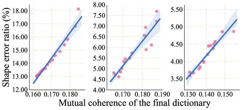
Figure 4: A scatter plot of the shape error ratio in percentage against the final dictionary coherence. A line is fitted based on the data. The left comes from subject 05, the middle from subject 18, the right from subject 64.

6 Conclusion

In this paper, we proposed multi-layer sparse coding as a novel prior assumption for representing 3D non-rigid shapes and designed an innovative encoder-decoder neural network to solve the problem of NRSfM using no 3D supervision. The proposed DNN was derived by generalizing the classical sparse coding algorithm ISTA to a block sparse scenario. The proposed DNN architecture is mathematically interpretable as a NRSfM multi-layer sparse dictionary learning problem. Extensive experiments demonstrated our superior performance against the state-of-the-art methods and the impressive generalization to unseen data. Finally, we propose to use the coherence of the final dictionary as a generalization measure, offering a practical way to avoid over-fitting and selecting the best model without 3D ground-truth.

(a) Subject 01.

(b) Subject 05.

(c) Subject 18.

(d) Subject 23.

(e) Subject 48.

(f) Subject 70.

(g) Subject 102.

(h) Subject 106.

(i) Subject 123.

(j) Subject 127.

(k) Failure case.

(l) Failure case.

Figure 5: Qualitative evaluation on reconstructed human skeletons. (a) to (j) are randomly selected from each subject. (k) and (l) are two failure cases with the largest errors among all 140,606 images. In each sub-figure, the left is the reconstruction of [8], the middle is the ground-truth, and the right is ours.

(m) Object table.

(n) Object sofa.

(o) Object chair.

(p) Object bed.

Figure 6: Qualitative results of SfC task. Reconstructions are randomly selected from each object category. Red cubes are reconstructed points while the planes and bars are manually added for descent rendering.

References

- [1] I. Akhter, Y. Sheikh, S. Khan, and T. Kanade. Trajectory space: A dual representation for nonrigid structure from motion. Pattern Analysis and Machine Intelligence, IEEE Transactions on, 33(7):1442–1456, 2011.
- [2] A. Beck and M. Teboulle. A fast iterative shrinkage-thresholding algorithm with application to wavelet-based image deblurring. In Acoustics, Speech and Signal Processing, 2009. ICASSP 2009. IEEE International Conference on, pages 693–696. IEEE, 2009.
- [3] C. Bregler, A. Hertzmann, and H. Biermann. Recovering non-rigid 3d shape from image streams. In Computer Vision and Pattern Recognition, 2000. Proceedings. IEEE Conference on, volume 2, pages 690–696. IEEE, 2000.
- [4] C. Cadena, A. R. Dick, and I. D. Reid. Multi-modal auto-encoders as joint estimators for robotics scene understanding. In Robotics: Science and Systems, 2016.
- [5] A. X. Chang, T. A. Funkhouser, L. J. Guibas, P. Hanrahan, Q. Huang, Z. Li, S. Savarese, M. Savva, S. Song, H. Su, J. Xiao, L. Yi, and F. Yu. Shapenet: An information-rich 3d model repository. CoRR, abs/1512.03012, 2015.
- [6] Z. Chen, V. Badrinarayanan, G. Drozdov, and A. Rabinovich. Estimating depth from rgb and sparse sensing. European Conference on Computer Vision (ECCV), 2018.
- [7] A. Chhatkuli, D. Pizarro, T. Collins, and A. Bartoli. Inextensible non-rigid shape-from-motion by second-order cone programming. In Proceedings of the IEEE Conference on Computer Vision and Pattern Recognition, pages 1719–1727, 2016.
- [8] Y. Dai, H. Li, and M. He. A simple prior-free method for non-rigid structure-from-motion factorization. International Journal of Computer Vision, 107(2):101–122, 2014.
- [9] I. Daubechies, M. Defrise, and C. De Mol. An iterative thresholding algorithm for linear inverse problems with a sparsity constraint. Communications on Pure and Applied Mathematics: A Journal Issued by the Courant Institute of Mathematical Sciences, 57(11):1413–1457, 2004.
- [10] A. Del Bue, F. Smeraldi, and L. Agapito. Non-rigid structure from motion using ranklet-based tracking and non-linear optimization. Image and Vision Computing, 25(3):297–310, 2007.
- [11] J. Deng, W. Dong, R. Socher, L.-J. Li, K. Li, and L. Fei-Fei. Imagenet: A large-scale hierarchical image database. In Computer Vision and Pattern Recognition, 2009. CVPR 2009. IEEE Conference on, pages 248–255. IEEE, 2009.
- [12] W. Deng, W. Yin, and Y. Zhang. Group sparse optimization by alternating direction method. In SPIE Optical Engineering+ Applications, pages 88580R–88580R. International Society for Optics and Photonics, 2013.
- [13] D. L. Donoho, M. Elad, and V. N. Temlyakov. Stable recovery of sparse overcomplete representations in the presence of noise. IEEE Transactions on information theory, 52(1):6–18, 2006.
- [14] P. F. Gotardo and A. M. Martinez. Computing smooth time trajectories for camera and deformable shape in structure from motion with occlusion. Pattern Analysis and Machine Intelligence, IEEE Transactions on, 33(10):2051–2065, 2011.
- [15] P. F. Gotardo and A. M. Martinez. Kernel non-rigid structure from motion. In Computer Vision (ICCV), 2011 IEEE International Conference on, pages 802–809. IEEE, 2011.
- [16] P. F. Gotardo and A. M. Martinez. Non-rigid structure from motion with complementary rank-3 spaces. 2011.
- [17] O. C. Hamsici, P. F. Gotardo, and A. M. Martinez. Learning spatially-smooth mappings in non-rigid structure from motion. In European Conference on Computer Vision, pages 260–273. Springer, 2012.
- [18] J. Huang and S. You. Point cloud labeling using 3d convolutional neural network. In Pattern Recognition (ICPR), 2016 23rd International Conference on, pages 2670–2675. IEEE, 2016.
- [19] C. Kong and S. Lucey. Prior-less compressible structure from motion. Computer Vision and Pattern Recognition (CVPR), 2016.
- [20] C. Kong, R. Zhu, H. Kiani, and S. Lucey. Structure from category: a generic and prior-less approach. International Conference on 3DVision (3DV), 2016.
- [21] S. Kumar, A. Cherian, Y. Dai, and H. Li. Scalable dense non-rigid structure-from-motion: A grassmannian perspective. arXiv preprint arXiv:1803.00233, 2018.
- [22] S. Kumar, Y. Dai, and H. Li. Multi-body non-rigid structure-from-motion. In 3D Vision (3DV), 2016 Fourth International Conference on, pages 148–156. IEEE, 2016.
- [23] M. Lee, J. Cho, and S. Oh. Consensus of non-rigid reconstructions. In Proceedings of the IEEE Conference on Computer Vision and Pattern Recognition, pages 4670–4678, 2016.
- [24] Y. Li, K. Qian, T. Huang, and J. Zhou. Depth estimation from monocular image and coarse depth points based on conditional gan. In MATEC Web of Conferences, volume 175, page 03055. EDP Sciences, 2018.
- [25] Y. Liao, L. Huang, Y. Wang, S. Kodagoda, Y. Yu, and Y. Liu. Parse geometry from a line: Monocular depth estimation with partial laser observation. In Robotics and Automation (ICRA), 2017 IEEE International Conference on, pages 5059–5066. IEEE, 2017.
- [26] J. J. Lim, H. Pirsiavash, and A. Torralba. Parsing IKEA Objects: Fine Pose Estimation. ICCV, 2013.
- [27] F. Mal and S. Karaman. Sparse-to-dense: Depth prediction from sparse depth samples and a single image. In 2018 IEEE International Conference on Robotics and Automation (ICRA), pages 1–8. IEEE, 2018.
- [28] M. Paladini, A. Del Bue, M. Stosic, M. Dodig, J. Xavier, and L. Agapito. Factorization for non-rigid and articulated structure using metric projections. In Computer Vision and Pattern Recognition, 2009. CVPR 2009. IEEE Conference on, pages 2898–2905. IEEE, 2009.
- [29] V. Papyan, Y. Romano, and M. Elad. Convolutional neural networks analyzed via convolutional sparse coding. The Journal of Machine Learning Research, 18(1):2887–2938, 2017.
- [30] C. R. Qi, H. Su, K. Mo, and L. J. Guibas. Pointnet: Deep learning on point sets for 3d classification and segmentation. Proc. Computer Vision and Pattern Recognition (CVPR), IEEE, 1(2):4, 2017.
- [31] V. Ramakrishna, T. Kanade, and Y. Sheikh. Reconstructing 3d human pose from 2d image landmarks. In European Conference on Computer Vision, pages 573–586. Springer, 2012.
- [32] C. J. Rozell, D. H. Johnson, R. G. Baraniuk, and B. A. Olshausen. Sparse coding via thresholding and local competition in neural circuits. Neural computation, 20(10):2526–2563, 2008.
- [33] H. Su, C. R. Qi, Y. Li, and L. J. Guibas. Render for cnn: Viewpoint estimation in images using cnns trained with rendered 3d model views. In Proceedings of the IEEE International Conference on Computer Vision, pages 2686–2694, 2015.
- [34] J. Sulam, V. Papyan, Y. Romano, and M. Elad. Multi-layer convolutional sparse modeling: Pursuit and dictionary learning. arXiv preprint arXiv:1708.08705, 2017.
- [35] J. Taylor, A. D. Jepson, and K. N. Kutulakos. Non-rigid structure from locally-rigid motion. IEEE, 2010.
- [36] L. Torresani, A. Hertzmann, and C. Bregler. Learning non-rigid 3d shape from 2d motion. In Advances in Neural Information Processing Systems, pages 1555–1562, 2004.
- [37] S. Vicente and L. Agapito. Soft inextensibility constraints for template-free non-rigid reconstruction. In European conference on computer vision, pages 426–440. Springer, 2012.
- [38] J. Wu, T. Xue, J. J. Lim, Y. Tian, J. B. Tenenbaum, A. Torralba, and W. T. Freeman. Single image 3d interpreter network. European Conference on Computer Vision (ECCV), 2016.
- [39] Z. Wu, S. Song, A. Khosla, F. Yu, L. Zhang, X. Tang, and J. Xiao. 3d shapenets: A deep representation for volumetric shapes. In Proceedings of the IEEE conference on computer vision and pattern recognition, pages 1912–1920, 2015.
- [40] X. Zhou, S. Leonardos, X. Hu, and K. Daniilidis. 3d shape estimation from 2d landmarks: A convex relaxation approach. In Proceedings of the IEEE Conference on Computer Vision and Pattern Recognition, pages 4447–4455, 2015.
- [41] Y. Zhu, D. Huang, F. D. L. Torre, and S. Lucey. Complex non-rigid motion 3d reconstruction by union of subspaces. In Computer Vision and Pattern Recognition (CVPR), 2014 IEEE Conference on, pages 1542–1549. IEEE, 2014.
- [42] Y. Zhu and S. Lucey. Convolutional sparse coding for trajectory reconstruction. Pattern Analysis and Machine Intelligence, IEEE Transactions on, 37(3):529–540, 2015.