Improved Representation of Ocean Heat Content in Energy Balance Models

Abstract

Anomaly-diffusing energy balance models (AD-EBM) are routinely employed to analyze and emulate the warming response of both observed and simulated Earth systems. We demonstrate a deficiency in common multi-layer as well as continuous-diffusion AD-EBM variants: They are unable to, simultaneously, properly represent surface warming and the vertical distribution of heat uptake. We show that this inability is due to the diffusion approximation. On the other hand, it is well understood that transport of water from the surface mixed layer into the ocean interior is achieved, in large part, by the process of ventilation—a process associated with outcropping isopycnals. We, therefore, start from a configuration of outcropping isopycnals and demonstrate how an AD-EBM can be modified to include the effect of ventilation on ocean uptake of anomalous radiative forcing. The resulting EBM is able to successfully represent both surface warming and the vertical distribution of heat uptake, and indeed, a simple four layer model suffices. The simplicity of the models notwithstanding, the analysis presented and the necessity of the modification highlight the role played by processes related to the down-welling branch of global ocean circulation in shaping the vertical distribution of ocean heat uptake.

1 Introduction

Energy balance models (EBM) have long been used in climate science as conceptual tools to understand heat transfer within the Earth system (e.g., Budyko, 1969; Sellers, 1969; Hoffert et al, 1980; Schneider and Thompson, 1981; North et al, 1981; Murphy, 1995; Gregory, 2000), as computationally-efficient emulators of and diagnostic tools for more complex Earth system models (ESMs) (Wigley and Raper, 1992; Raper and Cubasch, 1996; Houghton et al, 1997; Raper et al, 2001; Meinshausen et al, 2011a; Geoffroy et al, 2012), and to explore and quantify uncertainties in climate change projections (Urban and Keller, 2010; Padilla et al, 2011; Aldrin et al, 2012; Johansson et al, 2015; Bodman and Jones, 2016). EBMs represent changes in climate as the transfer of heat between appropriately aggregated units, and where the units are loosely referred to as layers when they are distributed in the vertical dimension alone (cf. isopycnal layers) and as boxes if other dimensions are involved as well. As an example of the former, in two-layer models that are widely used (e.g., see Schneider and Thompson, 1981; Gregory, 2000; Held et al, 2010, and references therein) both for climate projection purposes and to emulate Atmosphere-Ocean General Circulation Models (AOGCM), the atmosphere, the land surface, and the oceanic mixed layer components of the earth system are aggregated into one surface layer with a smaller thermal inertia and it interacts with a second layer that is representative of the sub-surface ocean and which has a larger thermal inertia. On the other hand, EBMs may allow for a coninuous representation in the relevant dimension (e.g., Budyko, 1969; Sellers, 1969; Raper et al, 2001; Meinshausen et al, 2011a, and others). Thus, in the context of upwelling-diffusion or pure-diffusion in the vertical, such EBMs consist of many layers (typically $\sim$40) with the intent of representing the limit of a continuous vertical dimension. Further combinations are easily realized.

In its use as a physics-based emulator, we would ask that an EBM be able to reproduce both ESM-simulated and observed surface and subsurface warming in a range of scenarios. Diffusion-class models have shown skill at reproducing observed surface warming and overall ocean warming as well as warming behaviors of ESMs under historical and future CO₂ emissions scenarios (e.g., see Gregory, 2000; Raper et al, 2001, 2002, and others). In particular, a popular form of a two-layer model has proven to be capable of capturing the typical two-timescale surface temperature response seen in abruptly forced AOGCM simulations (e.g., see Raper et al, 2001; Friend, 2011; Geoffroy et al, 2013, and others) across a range of AOGCMs. However, how well that model can represent the vertical structure of ocean heat uptake has not received much attention. We find that the two-layer model is unable to simultaneously properly represent surface warming responses and observational estimates of 0-700m and 700-2000m heat storage. Perhaps more surprising is that we find that more highly-resolved diffusion-class models are similarly deficient.

On the other hand, from the point of view of dynamical processes underlying global ocean circulation, this last finding—that vertically-resolved EBMs are unable to simultaneously fit both the surface response and the vertical distribution of ocean heat uptake—is not surprising for the following reasons: (a) From the point of view of ocean dynamics, it is well understood that transport of water from the surface mixed layer into the ocean interior is achieved, in large part, by the process of ventilation—a process associated with outcropping isopycnals. That is, when isopycnals outcrop at high latitudes, water masses that are at the surface at high latitudes are able to move laterally back to middle and low latitudes at deeper levels (e.g., see Chapter 4 of Pedlosky, 2013). (b) The deep ocean loses heat to the atmosphere at high latitudes through convective instabilities (e.g., see Chapter 7 of Talley, 2011), and when the stability of the water column is incrementally enhanced in a warming scenario (that is, the water column continues to remain unstable, but its degree of instability is slightly reduced), the heat loss from the deep ocean is slightly reduced leading effectively to a warming of the deep. Indeed, the effects of such processes have been verified in various climate models (e.g., see Gregory, 2000; Raper et al, 2001, 2002, and others).

Clearly, while there are many directions in which one could improve the realism of an EBM’s warming response, in this work we present one simple modification that enables simultaneously fitting a wide range of scenarios: Outcropping of isopycnals/neutral surfaces is a common feature of global ocean circulation (e.g., see Talley, 2011; Pedlosky, 2013). Nevertheless, this configuration has not received much attention in the context of EBMs. Indeed, we find that a cure to the problem identified in AD-EBMs lies in considering such a configuration. We, therefore, start from a conceptual configuration of outcropping isopycnals. Next, we perform a transformation of coordinates in order to cast this configuration into a framework of horizontally-averaged layers, a framework that is more commonly encountered in the EBM context. We then show mathematically that when such a configuration of outcropping isopycnal/neutral surfaces is viewed in terms of horizontally-averaged layers, non-local interactions between near-surface and deeper ocean layers result. We then show that such a modification, a modification that represents the lowest order effects of outcropping isopycnal/neutral surfaces, is sufficient to simultaneously capture surface warming and deeper ocean heat uptake. Indeed, we find that it is not necessary to use a fully one-dimensional model; a four-layer model suffices.

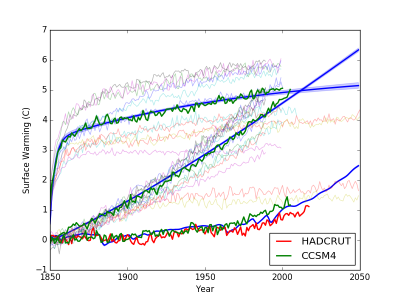
Figure 1: Here, the popular two layer EBM given by Eqs. 1 and 2 is calibrated against globally-averaged and annually-averaged SAT response of the CCSM4 model simulation of the abrupt4x CO₂ experiment of the CMIP5 protocol using a Bayesian framework. Mean and 95 percentile envelopes of the posterior predictive distribution of SAT using the calibrated SCM (blue) is compared against the SAT evolution in the full CCSM4 simulations for the 1% CO₂ and historical forcing experiments (green). The SAT response of a handful of other AOGCMs in the abrupt4x and 1% CO₂ forcing CMIP5 experiments are shown in lighter lines.

2 Methodology and Results

2.1 The Two-Layer EBM

A particular form of simple climate model (SCM) that has been popular in summarizing integral thermal properties of AOGCMs and ESMs is the anomaly-diffusing energy-balance model (AD-EBM) (e.g, see Schneider and Thompson (1981); Gregory (2000); Held et al (2010)). In this horizontally-integrated model of the climate system, the upper (surface) layer is comprised of the oceanic mixed layer, the atmosphere and the land surface and the bottom layer represents the ocean beneath the mixed layer. Evolution of the upper surface heat content anomaly per unit area is given by

$$C_{u}\frac{dT_{u}}{dt} ={\cal F}-\lambda T_{u}-\gamma\left(T_{u}-T_{d}\right)$$ (1)

where ${\cal F}$ represents the effective (anomalous) radiative forcing (e.g., as due to green-house gases recently), $\lambda$ represents the climate feedback parameter (e.g., see Knutti and Hegerl (2008)). Exchange of heat between the surface layer and the ocean beneath is parameterized by the difference in temperature between the two layers, with $\gamma$ being the constant of proportionality. Similarly, evolution of the subsurface ocean heat content (OHC) anomaly (again per unit area) is given by

$$C_{d}\frac{dT_{d}}{dt} =\gamma\left(T_{u}-T_{d}\right).$$ (2)

The heat capacities $C_{u}$ and $C_{d}$ can be equivalently expressed in terms of ocean layer depths, $h_{u}$ and $h_{d}$ as $C_{(\cdot)}=ch_{(\cdot)}$, where $c$ is the volumetric heat capacity with a nominal value of 4.1$\times$ 10⁶ Jm^-3K^-1.

2.2 Skillful Representation of Surface Warming in the Two-Layer EBM

This two-layer model has been used extensively for estimating climate sensitivity of AOGCMs and ESMs (e.g., see Held et al (2010); Geoffroy et al (2012), and others). Figure 1 shows an example of its typical use. In this figure, we have calibrated the four EBM parameters ($\lambda$, $\gamma$, $h_{u}$, $h_{d}$) using the Community Climate System Model v. 4.0 (CCSM4) AOGCM’s annual global surface air temperature (SAT) output from an abrupt CO₂ quadrupling (abrupt4x) experiment as the sole calibration data. The parameters are inferred probabilistically from the CCSM4 SAT time series using Bayesian Monte Carlo sampling, assuming a first-order autoregressive noise model to capture the AOGCM natural variability not represented in the EBM (e.g., as in Urban and Keller (2010) or Nadiga and Urban (2016); see online supplement section titled “Further Methodological Details” for further details). Bayesian inference allows us to explore the full set of EBM parameters that are capable of fitting the AOGCM SAT data, to ensure that our results are not fragile with respect to one particular choice of parameters.

Next, we validate the calibration of the two-layer model by considering new forcing scenarios—1%/year CO₂ increase and historical forcings. By propagating the, calibrated, joint posterior distribution of parameters, we produce posterior predictive distributions of the respective SAT responses. The SAT responses and their 95 percentile ranges are shown in Fig. 1 (see Sec. A of ES for further details). The good correspondence between the posterior predictive distribution of SAT in the 1% CO₂ (RMS error of 0.11 C) and historical forcing experiments (RMS error of 0.16 C), as compared to the corresponding AOGCM results attest to both the reasonableness and the usefulness of the model. The SAT response of a handful of other AOGCMs in the abrupt4x and 1% CO₂ forcing CMIP5 (Coupled Model Intercomparison Project Phase 5; Taylor et al (2012)) experiments (lighter lines) and the Hadley center estimate (HadCRUT4) are shown for future reference.

2.3 Ocean Heat Uptake Considerations

Use of SCMs like in the previous example is well established. However since in excess of 90% of the anomalous radiative forcing is sequestered in the world oceans (e.g., Domingues et al, 2008; Levitus et al, 2012; Balmaseda et al, 2013, and others) and since the nature of ocean heat uptake is important in determing surface response, we next examine the ability of the two-layer EBM to represent aspects of the ocean heat uptake. For this, the main data product we consider is the sequestration of heat in the top 700 m and between 700 m and 2 km in the global ocean, as provided by the National Oceanic Data Center (NODC) (Levitus et al, 2012). We compare these two observation-based timeseries against the corresponding timeseries in the SCMs.

We have considered a specific AOGCM, CCSM4, for our example here and it’s clear that we could have chosen any other AOGCM from the CMIP5 model ensemble. While the particular choice of the AOGCM whose response we use to calibrate the SCM will affect details of the results presented, we believe that the importance of this choice is secondary. Figure 1 shows in light lines the spread of SAT in the abrupt4x and 1% CO₂ CMIP5 experiments from a handful of other modeling centers as well. While there is considerable spread in the response of the different models in these experiments, the spread in the averaged response of the different models in the historical forcing simulations is much less given the required tuning of AOGCMs to best match the current state of the Earth’s climate system (e.g., Mauritsen et al, 2012). Multi-model AOGCM differences are therefore not likely to account for the ability of an SCM, fit to a particular AOGCM, to reproduce historical climate trends.

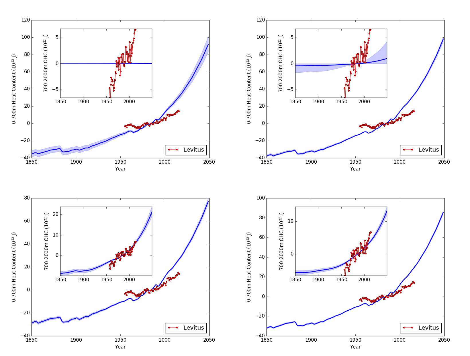
Figure 2: Comparison of the SCM representation of OHC against the observational estimate of 0-700m and 700-2000m OHC (Levitus et al, 2012). Top-left: two-layer EBM calibrated against CCSM4’s SAT response in the abrupt4x CMIP5 experiment. Top-right: calibrated against abrupt4x SAT and RN. Bottom-left: calibrated against abrupt4x SAT and RN and the observational estimates of OHC on using the historical forcing . Bottom-right: In a 60 layer model with calibration as in bottom-left.

In the top-left panel of Fig. 2, we compare the 0-700m (in the main plot) and 700-2000 m OHC (in the inset plot) in the previous experiment against the NODC (Levitus et al, 2012) observational estimates; again the posterior mean and 95% envelopes are shown. The SCM estimates are seen to fit the observational estimates very poorly.

This may not be surprising considering that in the previous experiment there was no constraint on heat storage in the climate system; as shown in Table. 1, calibration data comprised of only the surface warming in the abrupt4x AOGCM experiment. After all, the main motivation and the typical use of the two-layer EBM has been to capture the two timescales that are thought to characterize the surface warming response (e.g, see Gregory (2000) or Held et al (2010)).

2.4 Constraining the EBM’s Sub-surface Heat Content

Summing Eqs. 1 and 2 results in

$$\frac{d{\cal H}}{dt}={\cal F}-\lambda T_{u};\quad{\cal H}=c(h_{u}T_{u}+h_{d}T_{d})$$ (3)

and Eq. 3 represents the evolution of the heat content anomaly per unit area. The right hand side of Eq. 3 is the radiative imbalance (RI) or equivalently radiative non-equilibrium (RN).

Given the poor fit of OHC when the two-layer EBM is calibrated using the SAT response of the EBM in the abrupt4x experiment, we repeat the previous experiment, but now calibrating against both the SAT and radiative imbalance responses of the AOGCM. (A list of the experiments considered here is shown in Table 1; a few other supporting experiments discussed in the online supplement are shown in a table there.) While the SAT behavior is similar to that in Fig. 1 (not shown, but see Sec. 2 of supplement for figure and details), the OHC comparison is shown in the top-right panel of Fig. 2. It is seen that constraining the total heat storage leads to only minor improvements in the two layer EBM’s representation of ocean heat uptake. However, from the point of view of calibration itself, the differences are more dramatic: Not only are the EBM parameters inferred to be significantly different in the two experiments, but the inferences themselves are sharper and correlations that exist between model parameters in experiment 1 are seen to be greatly reduced in experiment 2 (see Sec. 2 of supplement for details).

2.5 A Shortcoming of the Two-Layer EBM

Since constraining overall heat storage in the abrupt4x CO₂ forcing experiment was seen to be insufficient to elicit an observationally-consistent heat storage response in the historical forcing experiment, we consider experiment 3, wherein we calibrate the two layer EBM against the AOGCM’s SAT and RN responses in the abrupt4x CO₂ forcing experiment, and calibrate against the observational estimate (0-700m and 700-2000m) of OHC itself, when the SCM is forced with an estimate of the historical forcing followed by the RCP8.5 scenario (Meinshausen et al, 2011b) to 2050.

In experiment 3, the simple two layer EBM’s representation of OHC (bottom left panel of Fig. 2) is seen to be better with improvements in the representation of the 700-2000m heat content. However, the 0-700m warming continues to be poorly represented. Attendant with the partial improvement in the representation of heat storage, unsurprisingly, is a slight degradation in the ability of the EBM to fit the SAT response in the abrupt4x CO₂ experiment (see Sec. 2 of supplement for further details and discussion).

We consider the inability of the two layer model to simultaneously properly represent the surface warming and the 0-700m and 700-2000m heat storage a shortcoming of the model and seek a simple extension of the model that will not suffer from this shortcoming. For brevity, when we refer to the problem or the shortcoming in the rest of the article, we are specifically referring to the shortcoming just described.

2.6 Persistence of the Shortcoming in Vertically-Resolved AD-EBMs

To investigate the possibility that it is the lack of resolution in the vertical that is the cause of the inability of the two layer EBM to represent heat storage in a manner that is consistent with observations, we considered a three layer extension and a four layer extension (experiment 4) of the two layer model. In each of these cases, calibration proceeded as in experiment 3. The close similarity in the SAT and heat storage responses of the three (not shown) and four layer models (see Table 1) to that in the two-layer suggests that a lack of resolution in the vertical may not be the direct cause of the problem.

Table 1: A brief overview of the experiments conducted. Units for RMS error of SAT is degrees C, and units for RMS error of OHC is $10^{22}$ J.

Expt. #	SCM	Calibration Details			RMS Error: SAT				OHC
		Forcing	AOGCM QoI	Obs. Data	4x	1%	HIS	OBS	$\leq$700	$>$700
1	2L	4x	SAT		0.13	0.11	0.16	0.18	7.5	3.2
2	2L	4x	SAT, RN		0.14	0.12	0.16	0.18	8.5	3.1
3	2L	4x	SAT, RN		0.21	0.14	0.16	0.18	5.8	1.5
		Historical		0-700m OHC	Degraded 4x SAT
				700-2000m OHC	Improved but Poor OHC
4	4L	4x	SAT, RN		0.17	0.13	0.16	0.18	5.7	1.4
		Historical		0-700m OHC	Reasonable SAT
				700-2000m OHC	Poor OHC
5	60L	4x	SAT, RN		0.18	0.13	0.16	0.18	6.5	1.7
	(many variants)	Historical		0-700m OHC	Reasonable SAT
				700-2000m OHC	Poor OHC
6	4LE	4x	SAT, RN		0.18	0.13	0.16	0.18	1.4	1.5
		Historical		0-700m OHC	Reasonable SAT
				700-2000m OHC	Reasonable OHC

Nevertheless, to probe the issue of vertical resolution further, we considered a number of variants of the continuously stratified version of the AD-EBM. A few of these experiments are detailed in the supplement under the section titled “Experiments with Continuous AD-EBM Variants”. (Bryan and Lewis, 1979; Nadiga and Urban, 2016). In these experiments, we typically discretized the subsurface thermocline region down to 2500 m into a series of layers of equal thickness since observational estimates of warming below 2000 m in the global ocean tend to be small (e.g., Cheng et al, 2017): $<$10% of the full ocean warming or $\lesssim$ 3$\times$ 10²² J currently. In these experiments, the main variations were in the form of vertical or diapycnal diffusivity assumed, and as to whether the coefficient(s) of diffusivity itself was (themselves were) fixed at realistic values or inferred in the calibration procedure. Other variations included fixing or inferring the depth of the upper layer and allowing for a (depth-independent) upwelling velocity or not (see supplement for details and results). Like in the other panels of Fig. 2, the bottom-right panel shows the OHC comparison for one such model that fit AOGCM responses and observational estimates of OHC best (Experiment 5g in supplement).

The improvements in going from a two-layer model to a large number of layers (here 60) is seen to be rather small. The inability of the continuously stratified AD-EBM may be understood as follows: In the suite of experiments conducted with the continuous model (and described in Sec. 3 of supplement), in the cases which fit AOGCM responses and observational estimates of OHC best, the inferred value of thermocline diffusivity ranged between 0.7 and 0.9 cm²/s. These values are much higher than the accepted levels of 0.1 cm²/s. One reason for these large values of vertical diffusivity is that the model is attempting to get sufficient heat down to the 700-2000 m depths in order to satisfy the observational constraint. And in trying to do so, it is clear from these experiments that this is causing too large a heating in the 0-700 m depth range—a feature that is consistent across a wide suite of experiments (described in Sec. 3 of supplement). That is, assuming that vertical diffusivity is not varying with time (and there is no reason to expect it to have varied substantially with time in the post industrial period) getting observed levels of warming into the 700-2000 m layer while limiting the warming of the 0-700m layer to observed levels is difficult to achieve in AD-EBMs.

2.7 Moving Beyond Diffusion of Anomalies: Outcropping Surfaces

The inability of the continous variants of AD-EBM model to reasonably represent the vertical distribution of OHC leads us to next consider if it is the anomaly diffusion aspect of these models that prevents the SCM from being able to simultaneously properly represent surface warming and the 0-700m and 700-2000m heat storage. After all, the global ocean circulation tends to be highly dynamic in the sense that it is largely adiabatic outside of the surface layer and bottom boundary layers, and an anomaly diffusing model attempts to parameterize the horizontally-averaged effect of the myriad dynamical processes through diffusion across adjoining layers. This may be restrictive in the sense that the effect of processes such as deep-water formation, and subduction and mode water formation processes on ocean heat storage, when averaged horizontally, may no longer appear as local diffusion operators. For example, when water in the midlatitudes whose properties are set by its last interaction with the atmosphere slides down an appropriate isopycnal, in a horizontally averaged sense this process will appear as if two non-adjoining layers are interacting.

Figure 3: Model schematic: In the meridional-depth plane (not to scale) outcropping isopycnal/neutral surfaces are show in thin continuous curved lines. These are then idealized into horizontal and vertical surfaces shown in thick continuous straight lines. Finally the horizontally-averaged layers are shown in dashed straight lines. We demonstrate mathematically that purely local interactions in the isopycnal/neutral coordinates lead to non-local interactions when horizontally-averaged layers are considered.

To demonstrate this effect, consider a schematic of the meridional-depth cross-section of the world oceans, as shown in Fig. 3. In this figure, the outcropping isopycnal/neutral surfaces in thin continuous lines are idealized into the horizontal and vertical surfaces shown in thick continuous lines. In Fig. 3, $\alpha_{i}$ is the meridional fraction of layer $i$ that outcrops and is exposed to the atmosphere. The EBM for such layers is:

$$c\left(\alpha_{i}\sum_{j=1}^{i-1}h_{j}+h_{i}\sum_{j=1}^{i}\alpha_{j}\right)\frac{d{T_{i}}}{dt}=\alpha_{i}\left({\cal F}-\lambda T_{i}\right)+\sum_{j=\max(1,i-1)}^{\min(N,i+1)}\gamma_{ij}(T_{j}-T_{i})$$ (4)

and where $\gamma_{ij}$ ($=\gamma_{ji}$) parameterizes the interactions between adjoining layers $i$ and $j$ and the summation terms drop to 0 when the starting lower index is greater than the ending upper index.

With trivial manipulation, Eq. 4 can be rewritten in a compact symbolic form as

$$\frac{d{T}}{dt}=C+AT$$ (5)

where $T$ is the vector of temperatures $T_{i}$ in Eq. 4, $C$ is a constant vector related to the anomalous radiative forcing and $A$ is a tridiagonal matrix that is independent of $T$. (Note that $A$ in Eq. 5 is not symmetric even though the right hand side of Eq. 4 is. This is because each row of the matrix form of Eq. 4 gets divided by a different constant (the coefficient of $\frac{d{T}}{dt}$) in Eq. 4.) Next, consider horizontal averaging of temperature in Fig. 3 to go from the idealized outcropping layers (shown in thick continuous lines) to horizontally-averaged layers (shown in dashed lines):

$$\sum_{j=i+1}^{N}\alpha_{j}T_{j}+T_{i}\sum_{j=1}^{i}\alpha_{j}=\widetilde{T}_{i}$$ (6)

where $\widetilde{T}_{i}$ is the temperature of the $i^{th}$ horizontally-averaged layer, and again the same rules hold for summation. Again, Eq. 6 can be written in a compact form as:

$$BT=\widetilde{T}$$ (7)

where by virtue of the limits of the summation in the first term on the left hand side of Eq. 6, $B$ is seen to be upper triangular. In the generic case of $\sum_{j=1}^{i}\alpha_{j}\neq 0$, Eq. 7 can be inverted as

$$T=B^{-1}\widetilde{T}.$$ (8)

$B^{-1}$ is upper triangular because $B$ is upper triangular. Inserting Eq. 8 in Eq. 5 and simplifying leads to

$$\frac{d\widetilde{T}}{dt}=\widetilde{C}+\widetilde{A}\widetilde{T}.$$ (9)

While $A$ is tridiagonal (see Eq. 4), $\widetilde{A}$ is not: To see that $\widetilde{A}$ is not tridiagonal, consider that

$$\widetilde{A}_{ij}=\sum_{k=1}^{n}\sum_{l=1}^{n}B_{ik}A_{kl}B^{-1}_{lj}=\sum_{k=i}^{n}\sum_{l=1}^{j}B_{ik}A_{kl}B^{-1}_{lj}$$ (10)

where the second equality is due to the upper triangular nature of $B$ and ${B}^{-1}$ ($B_{ij}=B_{ij}^{-1}=0$ for $i>j$). Therefore if $i>j+1$, the values of $k$ and $l$ in the above sum satisfy the inequality $k\geq i>j+1\geq l+1$, meaning that $k>l+1$. Therefore $A_{kl}=0$ for all the terms in the above sum for $i>j+1$, making ${\widetilde{A}}_{ij}=0$ for $i>j+1$.

That is while the outcropping isopycnal/neutral layers interact purely locally in isopycnal/neutral coordinates (tridiagonal $A$ in Eq. 5), the same dynamic when represented using horizontally averaged layers leads to nonlocal interactions (e.g., the top layer interacts with as many of the underlying layers as there are outcropping isopycnals.)

2.8 Results with the Modified EBM

Following the mathematical development above, we next evaluate if the modified EBM given by Eq. 9 is capable of overcoming the shortcoming identified in the AD-EBMs. As previously mentioned, $\widetilde{A}$ not being tridiagonal amounts to allowing for interactions between non-adjoining, horizontally-averaged layers. As for adjoining layers, we again parameterize such interactions in terms of the difference in their temperature anomalies. The simplest extension then consists of a three layer model with a new interaction between the top layer and the deepest layer. Within the range of experimentation that we conducted, we find that such a three layer extension is incapable of adequately resolving the shortcoming; for that we need at least four layers.

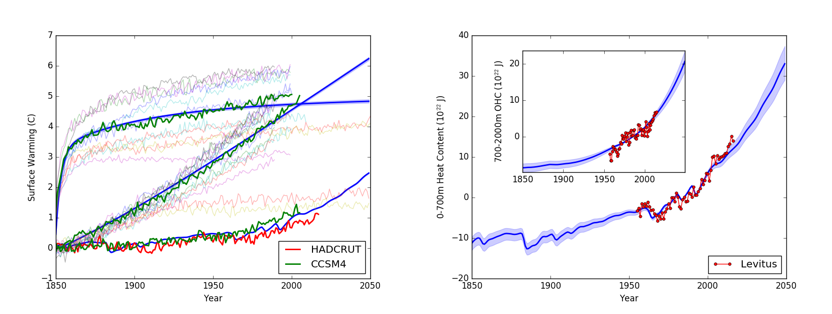
Figure 4: In Experiment 6, a four layer model with non-local interactions is seen to be able to simultaneously represent surface warming and the 0-700m and 700-2000m heat storage in a reasonable fashion.

Figure. 4 shows the response of such an extended four layer model (Expt. 6 in Table. 1). Both SAT and OHC representations are reasonable enough to suggest that this is a simple extension of the two layer EBM that overcomes the shortcoming of the latter of not being able to simultaneously represent the surface responses and subsurface ocean heat uptake in a variety of settings.

3 Discussion and Conclusions

Simple climate models play a valuable role in helping interpret both observations and responses of comprehensive earth system models. To this end, we considered the anomaly-diffusion energy balance model and used it in a Bayesian framework to interpret a few CMIP5 experiments—the abrupt 4$\times$CO₂ forcing, the 1% CO₂ forcing and the historical forcing experiments. The intention of the CMIP abrupt 4$\times$CO₂ forcing experiment is one of calibration and diagnosis of equilibrium climate sensitivity since post-industrial surface warming itself is compatible with a wide range of climate sensitivities. As such, we used the abrupt 4$\times$CO₂ forcing CCSM4 experiment in conjunction with an observational estimate of OHC to infer the SCM parameters and used those parameters to compute the SCM responses to other forcings. We demonstrated that the commonly-used anomaly-diffusing energy balance SCM is deficient in being unable to simultaneously properly represent the SAT responses and observational estimates of OHC from NODC.

After verifying that this deficiency is not related to vertical resolution, we considered the possibility that it is due to the anomaly diffusion approximation. To this end, we demonstrated mathematically that when outcropping isopycnals are considered in a framework of horizontally-averaged layers, the outcropping of isopycnals leads to non-local interactions in the framework of horizontally-averaged layers. With this modification, we then showed that four layers were sufficient to successfully resolve the shortcoming of the AD-EBM class of SCMs. We also go on to show that that with such apparent non-local interactions—see supplement section “Further Experiments with Non Local Interactions” for a particular form—a continuous version of the model is similarly able to successfully resolve the shortcoming.

It is possible, however, that other kinds of augmentations to the commonly-used AD-EBM may fix the identified deficiency as well. On the other hand, since the simple extension that allows for simultaneously properly representing the surface warming and the 0-700m and 700-2000m heat storage is consistent with the effects of processes such as subduction and mode water formation and deepwater formation on ocean heat storage, our finding may be interpreted as indicative of the importance of direct sequestration of heat in the vertical interior of the world oceans by such processes. In particular, and as discussed in the introduction, since the (deep) ocean loses heat to the atmosphere at high latitudes through convective instabilities, when the stability of the water column is incrementally enhanced in a warming scenario (that is, the water column continues to remain unstable, but its degree of instability is slightly reduced), the heat loss from the deep ocean is slightly reduced leading effectively to a warming of the deep. At the next order, the resulting slowdown of the overturning circulation itself would further affect the heat uptake. Indeed, to examine such effects, we note that in ongoing work we consider extensions to a class of models that are used to study the overturning circulation (Tziperman, 1986; Gnanadesikan, 1999; Goodwin, 2012; Marshall and Zanna, 2014) to simultaneously represent surface warming and deeper ocean warming.

In both the four-layer and continuous variants of the EBM with non-local interactions, we also find that being able to reasonably represent the surface response and the 0-2000 m OHC is often associated with heat storage at depths below 2000 m that is greater than 10%. Clearly this finding needs to be investigated further in a hierarchical framework—a framework that will allow us to infer model parameters using the multi-model CMIP5 ensemble. In ongoing work, we are also examining (a) the implications of this study on estimates of uncertainty of climate sensitivity and (b) if these modified SCMs will help in better analyzing and inter-comparing ESMs.

Supplementary Material

∎

Improved Representation of Ocean Heat Content in Energy Balance Models. Supplementary Material B.T. Nadiga and N.M. Urban

Appendix A Further Methodological Details

EBMs have been used extensively to obtain estimates of Equilibrium Climate Sensitivity (ECS) of AOGCMs and ESMs. However, unlike the comprehensive AOGCMs and ESMs, the simpler of the EBMs such as the ones considered in this article do not represent natural climate variability. For this reason, the Bayesian calibration procedure requires the specification of a structure for natural variability. For example, for the temperature of the upper layer, $T_{u}$,

$$T_{u}^{ESM}(t)=T_{u}^{EBM}(t)+\epsilon_{t},$$ (11)

where $\epsilon_{t}$ is the discrepancy and similarly for other variables such as radiative imbalance and ocean heat content. Depending on the variable, the discrepancy structure can be reasonably approximated by simple stochastic processes such as independent and identically distributed (iid), auto-regressive processes (AR; e.g., AR(1)) or Gaussian Processes (GP). As mentioned in the main body, we used AR(1) for each of the variables considered in the Bayesian calibration procedure.

There is, however, a dependency of parameter estimates and their uncertainties on the assumed temporal structure of the discrepancy. Likewise, how the posterior distribution of calibrated responses match the original data (observational estimates or ESM responses) depends on the discrepancy model used. See Nadiga and Urban (2016) for an example of how ECS estimates and their uncertainty depends on the structure assumed for the discrepancy in the context of the two-layer EBM considered here.

Even after the structure of the discrepancy model is assumed, the results of the Bayesian inference procedure depend on whether the parameters of the discrepancy model are specified or inferred. A number of the experiments presented here were performed both ways: once while inferring, also, the parameters of the AR(1) model and a second time while specifying the parameters of the AR(1) model after first fitting that particular response alone using least-squares (i.e., after obtaining a point estimate of only the EBM parameters). In most of the cases, we found that attempting to infer the parameters of the AR(1) model simultaneously led to issues of identifiability. That is, for a significant number of the parameters related to the discrepancy model that we were, also, trying to infer, the calibration data were unable to move the prior distribution of that parameter. That is, for these parameters, the posterior distribution remained very close to the specified prior distribution. Consequently, the width of the assumed uninformative priors for these parameters led to further augmenting uncertainties in the EBM parameters. For this reason, it was deemed more appropriate to perform the inferences while specifying the parameters for the discrepancy model.

The covariance structure for the AR(1) process can be written as

$$\Sigma(t-s)=\sigma^{2}\rho^{|t-s|}$$ (12)

The specified values of $\sigma$ and $\rho$ were as follows abrupt4x SAT: (0.15 K, 0.5); abrupt4x RN: (0.27 W/m², 0.1); 0-700 m OHC: (2 $\times 10^{22}$ J, 0.8); 700-2000 m OHC: (1 $\times 10^{22}$ J, 0.8). This is consistent with the anamolous forcing varying fastest, the SAT response which is an integrated response to the anamolous forcing varying on a slower time scale related to the lower heat capacity of the upper layer and the OHC varying slowest because of its higher heat capacity. There may be legitimate reasons to consider other values for these parameters. Further experimentation was conducted along these lines. Results of such experimentation suggest that there may be a tradeoff between fitting the various pieces of calibration data but that such tradeoff will not affect the overall nature of our results and conclusions.

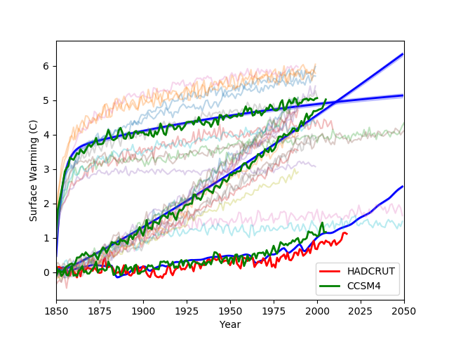
Figure 5: SAT responses of the two-layer EBM in experiments 2 and 3.

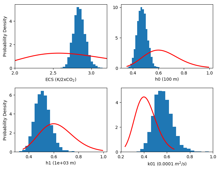
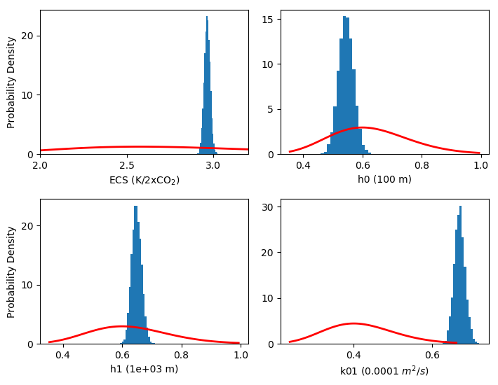
Figure 6: Prior (red curves) and posterior (blue histograms) distribution of the four model parameters in the two layer EBM in experiments 1 (left) & 2 (right). Constraining the overall heat storage in experiment 2 leads to slight changes in mode of the inferred parameters, but to large reductions in the width of the posteriors.

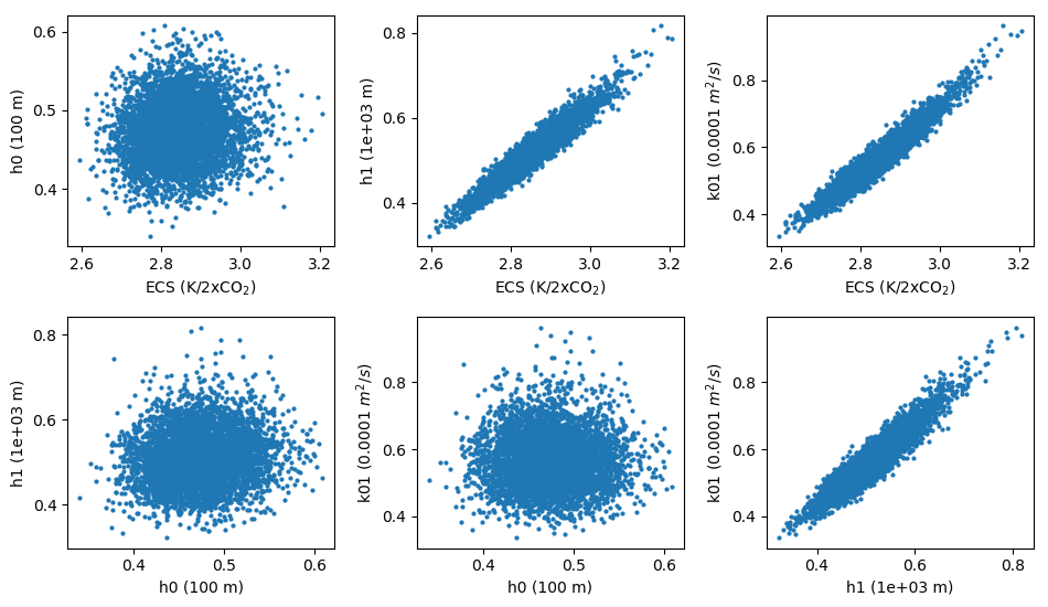
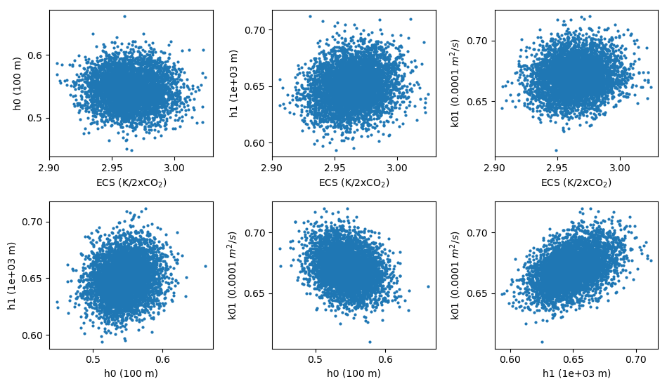
Figure 7: Posterior parameter correlations in experiments 1 & 2. Constraining the overall heat storage in experiment 2 leads to removal of the correlations seen in experiment 1 to a large extent.

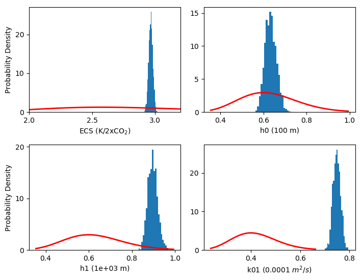
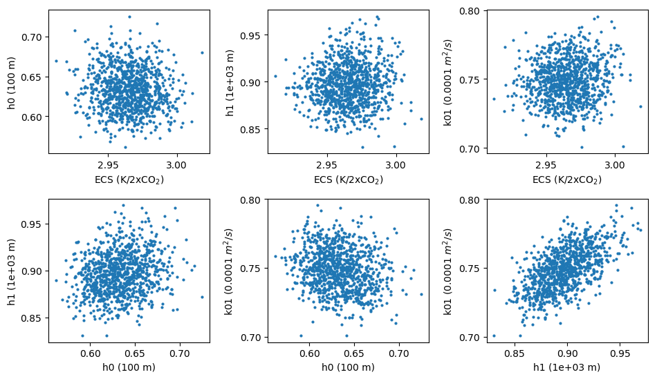
Figure 8: Parameter distributions, and correlations in experiment 3. Constrainting 0-700 m and 700-2000 m OHC leads to further changes in the inferred two-layer EBM parameters, but as discussed in Sec. 2, the two-layer EBM is unable to reasonably fit the observational estimates of OHC.

Appendix B Further Two-Layer EBM Details

As mentioned in Sec. 2 of the article and seen in the top row of Fig. 2 of the article, while there are differences in representation of OHC in the two-layer EBM in experiments 1 and 2, these differences are not dramatic. For completeness, the SAT response is shown in the left panel of Fig. 5 and the differences in the SAT responses are seen to be minor as well.

However, constraining the total heat storage in the climate system in experiment 2 by calibrating against the radiative imbalance/nonequilibrium (RI/RN) response of the ESM results in significant changes to the inferred (posterior) distributions of the SCM parameters. As seen in Fig. 6, using the RN constraint leads to the inferred EBM parameters being significantly different. It is also seen in that figure that the posterior distributions themselves are much narrower.

Furthermore, correlations that exist between model parameters in experiment 1 are seen to be greatly reduced in experiment 2 (see Fig. 7).

For completeness, SAT responses in experiment 3 is shown in the right panel of Fig. 1 and the parameter distributions, and their correlations in experiment 3 are shown in Fig. 8.

Expt. #	SCM	Comment
5a	40L; MLD inferred
	$\kappa_{v}^{TC}$ inferred	Degraded 4x SAT
	$\kappa_{v}^{ML_{bot}}=\kappa_{v}^{TC}$	Poor OHC
5b	40L	Degraded 4x SAT
	MLD = 70 m	Poor OHC
5c	40L	Degraded 4x SAT
	$\kappa_{v}^{ML_{bot}}\neq\kappa_{v}^{TC}$
	$\kappa_{v}^{ML_{bot}},\kappa_{v}^{TC}$ inferred	Poor OHC
5d	40L	Poor SAT
	$\kappa_{v}^{TC}=10^{-5}$ m2/s	Poor RN
	$\kappa_{v}^{ML_{bot}}\neq\kappa_{v}^{TC}$	Poor OHC
5e	40L; w inferred	Same as in Expt. 5c
	$\kappa_{v}^{ML_{bot}}\neq\kappa_{v}^{TC}$	Degraded 4x SAT
	$\kappa_{v}^{ML_{bot}},\kappa_{v}^{TC}$ inferred	Poor OHC
5f	40L; $\kappa_{v}^{>650m}$ inferred	Same as in Expt. 5c
	$\kappa_{v}^{ML_{bot}}\neq\kappa_{v}^{TC}$	Degraded 4x SAT
	$\kappa_{v}^{ML_{bot}},\kappa_{v}^{TC}$ inferred	Poor OHC
5g	60L; Same as 5c	Same as in Expt. 5c
7a	40L; Same as 5c	Reasonable SAT
	Non-local interaction	Reasonable OHC
7b	60L; Same as 5c/g/7	Same as in Expt. 7a
	Non-local interaction

Table 2: Some of the continuous AD-EBM variants considered

Expt.	SAT RMS Error				OHC RMS Error
	4x	1%	Hi	HC	0-700m	700-2000m
5a	0.19	0.11	0.16	0.17	7.5	2.2
5b	0.26	0.12	0.16	0.16	8.2	2.3
5c	0.18	0.13	0.16	0.18	6.5	1.7
5d	0.39	0.14	0.15	0.17	7.0	3.1
5e	0.16	0.13	0.16	0.18	5.9	1.4
5f	0.17	0.13	0.16	0.18	6.5	1.7
5g	0.18	0.13	0.16	0.18	6.5	1.7
7a	0.15	0.12	0.16	0.18	2.0	1.5
7b	0.15	0.12	0.16	0.18	1.6	1.5

Table 3: RMS error of SAT, with respect to CCSM4 experiments abrupt4x, 1%, historical forcing, and with respect to HadCRUT, and RMS error of OHC with respect to 0-700m and 700-2000m estimates from NODC in historical-forcing runs. Units for RMS error of SAT is degrees C, and units for RMS error of OHC is $10^{22}$ J.

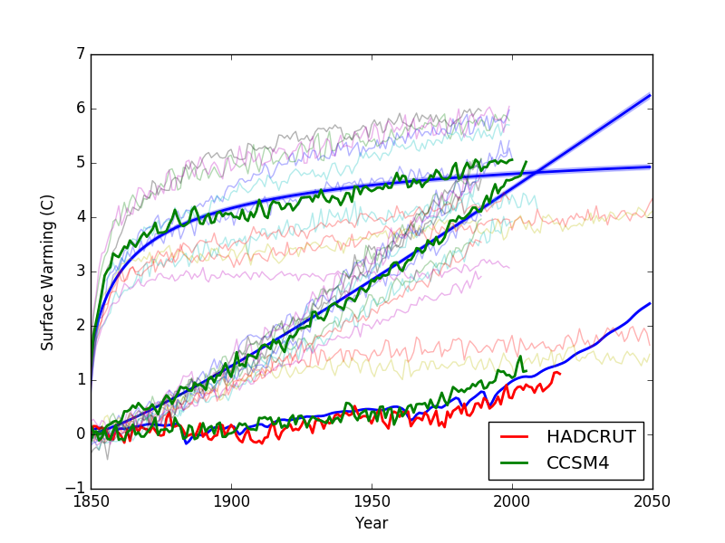
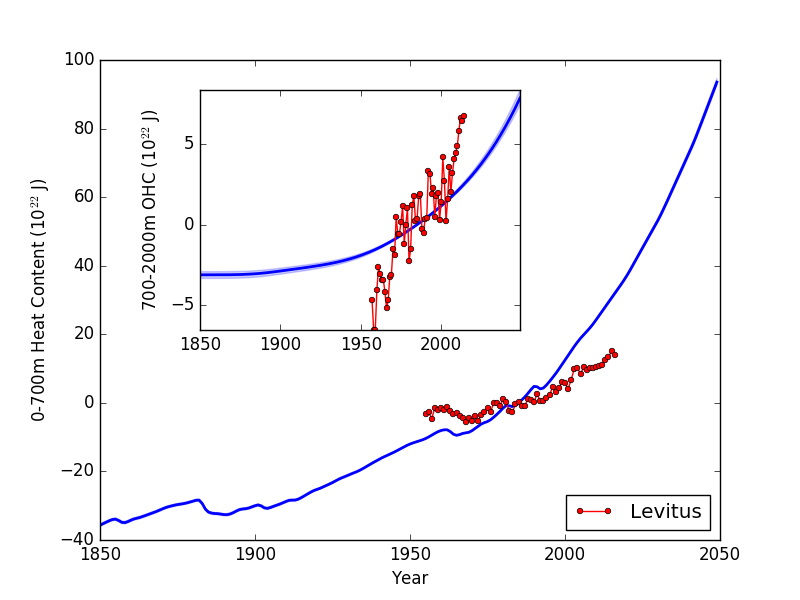
Figure 9: In Experiment 5a, allowing 40 layers in the AD-EBM model does not help improve the reprsentation of OHC.

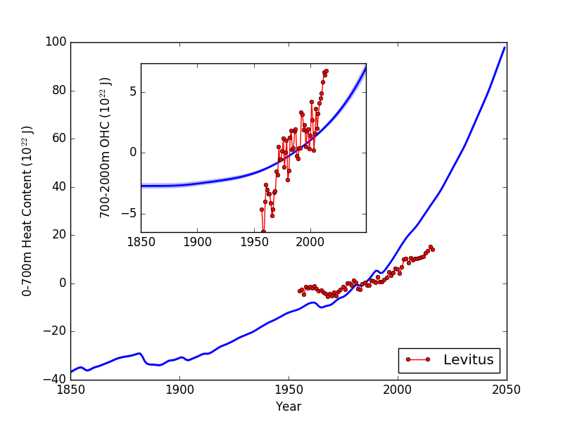
Figure 10: In experiment 5b, a variant of experiment 5a, the upper layer depth is held fixed at 70 m. This does not help improve the OHC response and the results are similar to that of experiment 5a.

Figure 11: In Experiment 5c, it is seen that allowing vertical diffusivity at the bottom of the ML to be different from its thermocline value leads to improvement in the SCM response. However, the improved response is comparable to that of the two-layer EBM and suffers from similar shortcomings.

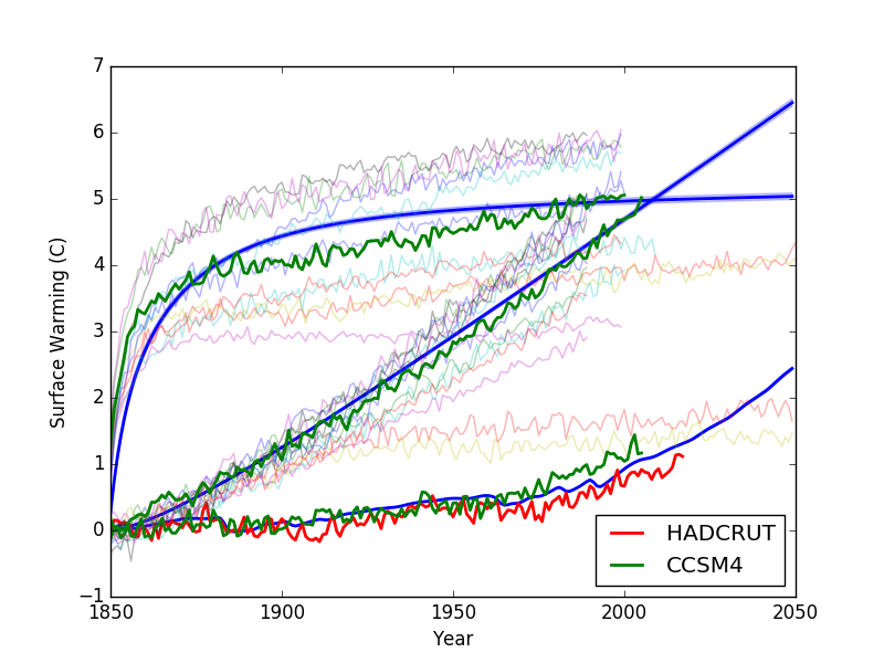
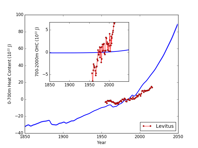
Figure 12: In Experiment 5d, a variant of experiment 5c, the thermocline diffusivity is set at a realistic value of 10^-5 m²/s. While not helping improve the representation of OHC, the SAT response in the abrupt4x case is seen to be degraded.

Figure 13: In Experiment 5e, a variant of experiment 5c, a depth-independent upwelling velocity is allowed. Allowing upwelling does not seem to help improve the representation of OHC.

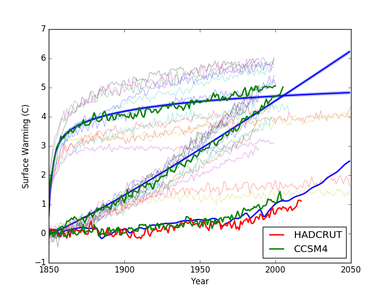
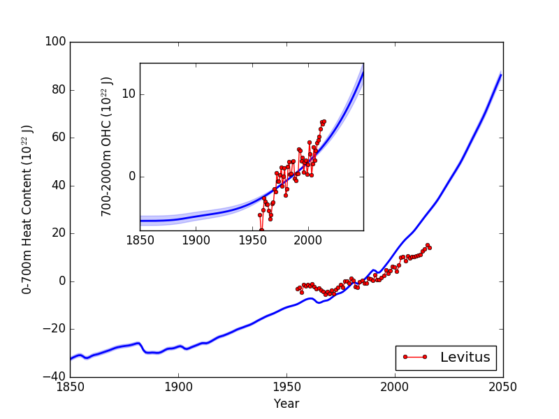
Figure 14: In Experiment 5f, a variant of experiment 5c, the vertical diffusivity below 650 m is allowed to take on a different inferred value. Again the differences in responses from 5c are seen to be minor.

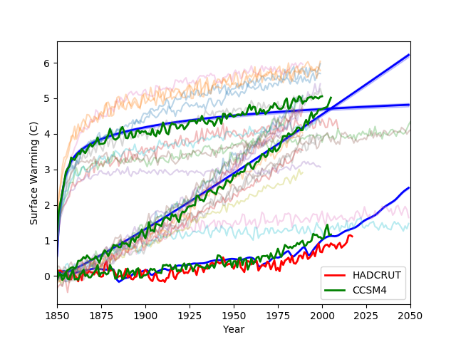
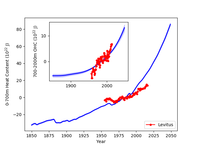
Figure 15: In Experiment 5g, a variant of experiment 5c, the number of layers is increased to 60. The differences in responses from 5c are seen to be very minor.

Appendix C Experiments with Continuous AD-EBM Variants

Table. 3 lists some of the continuous variants of AD-EBM discussed here. We note that the calibration procedure in each of these experiments were identical to that in Experiment 3 (see Table 1). In the first version (Experiment 5a), we consider a variable thickness top layer and discretize the sub-surface thermocline region down to 2500 m into 39 equi-depth layers. Figure 9 shows that the continuously-stratified AD-EBM suffers from a similar shortcoming in not being able to simultaneously properly represent surface warming and the 0-700m and 700-2000m heat storage.

In Experiment 5a, the thickness of the top layer in the continuously stratified AD-EBM was seen to be very shallow ($\sim$ 10 m). For this reason, we conduct Experiment 5b in which the thickness of the top layer is fixed at 70 m. The SAT and OHC behavior is shown in Fig. 10. Fixing the top layer depth at a reasonable value seem to have little effect on the representation of heat storage, and the results are similar to that in Experiment 5a.

In Experiment 5c, the vertical diffusivity at the bottom of the top layer is allowed to be different from its thermocline value in order to see if this will permit a better representation of ocean heat content. Significant improvements are indeed seen in the responses of the SCM and qualitatively, these responses are similar to those in the two-layer model. Indeed, the results of this experiment seem to strongly suggest that the continuously-stratified AD-EBM suffers from a similar shortcoming in not being able to simultaneously properly represent surface warming and the 0-700m and 700-2000m heat storage.

Next, we consider vertical diffusivity to have realistic values of 10^-5 m²/s in the thermocline and 10^-4 m²/s in the abyssal ocean with a vertical profile following Bryan and Lewis, 1979. However, the transition from the thermocline value to the abyssal value occurs (and is conventionally thought to be so) at 2500 m. As discussed in the main body, observational estimates of present day heating below 2000 m is small and so, in Experiment 5d, the value of vertical diffusivity is fixed at the thermocline value of 10^-5 m²/s. Experiment 5d was among the worst in being able to match the ESM responses and the observed estimates of OHC.

Experiment 5e differs from Experiment 5c in allowing for a depth-independent upwelling velocity that is inferred in the Bayesian calibration procedure. The degree of mismatch between the SCM responses and the ESM responses and observational estimates of OHC are similar to that in Experiment 5c.

In experiment 5f, a variant of 5c, we allow the diffusivity to take on a different value below 650 m. This was motivated more by the nature of the observational estimate of OHC rather than physics. However, only minor differences are seen with respect to experiment 5c.

In Experiment 5g, we increase the number of layers in the thermocline to 60, and Fig. 15, demonstrates convergent behavior of the inability to simultaneously properly represent surface warming and the 0-700m and 700-2000m heat storage in the continuously stratified AD- EBM.

The inability of the continuously stratified AD-EBM may be understood as follows: Experiment 5c (equivalently 5g) fits ESM responses and observational estimates of OHC best. The inferred value of thermocline diffusivity in these cases range between 0.7 and 0.9 cm²/s. These values are much higher than the accepted levels of 0.1 cm²/s. One reason for these large values of vertical diffusivity is that the model is attempting to get sufficient heat down to the 700-2000 m depths in order to satisfy the observational constraint. And in trying to do so, it is clear from these experiments that this is causing too large a heating in the 0-700 m depths—a feature that is consistent across a number of the experiments described here. That is, assuming that vertical diffusivity is not varying with time (and there is no reason to expect it to have varied substantially with time in the post industrial period) getting observed levels of warming into the 700-2000 m layer while limiting the warming of the 0-700m layer to observed levels is difficult to achieve in the AD-EBM.

Appendix D Further Experiments with Non Local Interactions

We next consider a modification of the continuous version of the AD-EBM that addresses the deficiency. In the original approach of Hoffert, 1980 to the AD-EBM, the direct sequestration of heat by the polar downwelling branch in the cartoon of the overturning circulation in the world oceans is not considered; only the effect of the resultant weak and broad upwelling is considered. We hypothesize that the deficiency of the AD-EBM identified above can be remedied by introducing a parameterization of the direct sequestration of heat by processes related to polar downwelling in the AD-EBM. To test this hypothesis, we consider a parameterization of the direct sequestration of heat by polar downwelling, and in anology with the formation of the North Atlantic Deep Waters. The structure of a nominal overturning cell in which the NADW is a component has a maximum in the overturning streamfunction around a km in depth. Consequently, we consider a profile of exchange of heat between the first sub-surface layer and the interior that has a Gaussian profile in the vertical centered at $z_{mx}$ and a vertical scale of $\Delta z$, and where both $z_{mx}$ and $\Delta z$ are inferred. That is, the anomaly-diffusion nature of the thermocline is augmented as

$$\frac{\partial T}{\partial t}+w\frac{\partial T}{\partial z}=\frac{\partial}{\partial z}\left(\kappa(z)\frac{\partial T}{\partial z}\right)+\gamma_{d}\exp\left(-\frac{(z-z_{mx})^{2}}{\Delta z^{2}}\right)(T_{1}-T).$$

Here $\gamma_{d}$ is a scalar coefficient of heat exchange associated with the parameterization and is inferred in the calibration process. Figure 16 shows that the SAT and OHC responses are fit reasonably in the model. Furthermore, in this simplified parameterization, if half of the depth $z_{mx}$ is taken as the depth at which the maximum of the overturning streamfunction occurs, the maximum overturning depth is inferred to lie at about a km, which is somewhat realistic. Finally, in Fig. 17, it is seen that the changes are minimal when the number of vertical layers is increased from 40 to 60.

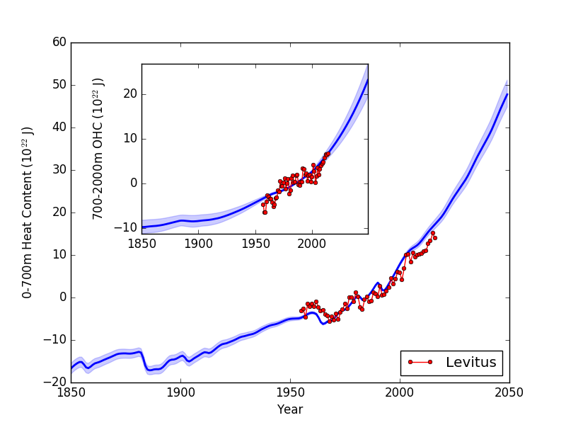
Figure 16: In Experiment 7a, a modification of the continuously-stratified model to allow for a non-local interaction—motivated by the direct sequestration of heat by deepwater formation processes—is seen to be able to simultaneously represent surface warming and the 0-700m and 700-2000m heat storage in a reasonable fashion.

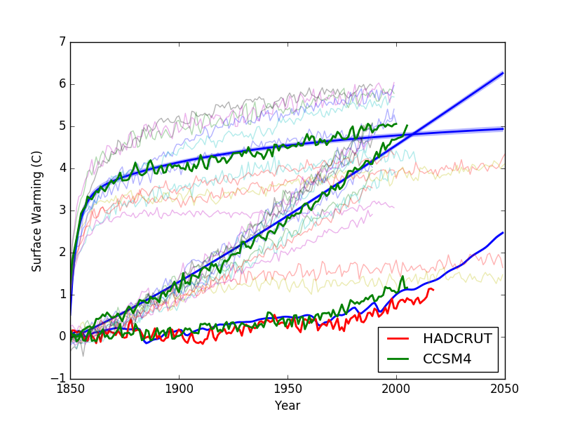
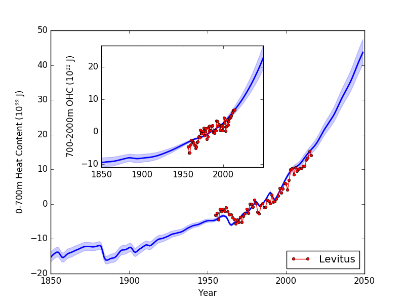
Figure 17: In Experiment 7b, a variant of experiment 7, that has 60 layers in the vertical, a convergent behavior with respect to increasing vertical resolution is seen.

References

- Aldrin et al (2012) Aldrin M, Holden M, Guttorp P, Skeie RB, Myhre G, Berntsen TK (2012) Bayesian estimation of climate sensitivity based on a simple climate model fitted to observations of hemispheric temperatures and global ocean heat content. Environmetrics 23(3):253–271
- Balmaseda et al (2013) Balmaseda MA, Trenberth KE, Källén E (2013) Distinctive climate signals in reanalysis of global ocean heat content. Geophysical Research Letters 40(9):1754–1759
- Bodman and Jones (2016) Bodman RW, Jones RN (2016) Bayesian estimation of climate sensitivity using observationally constrained simple climate models. Wiley Interdisciplinary Reviews: Climate Change 7(3):461–473
- Bryan and Lewis (1979) Bryan K, Lewis L (1979) A water mass model of the world ocean. Journal of Geophysical Research: Oceans 84(C5):2503–2517
- Budyko (1969) Budyko MI (1969) The effect of solar radiation variations on the climate of the earth. Tellus 21(5):611–619
- Cheng et al (2017) Cheng L, Trenberth KE, Fasullo J, Boyer T, Abraham J, Zhu J (2017) Improved estimates of ocean heat content from 1960 to 2015. Science Advances 3(3):e1601,545
- Domingues et al (2008) Domingues CM, Church JA, White NJ, Gleckler PJ, Wijffels SE, Barker PM, Dunn JR (2008) Improved estimates of upper-ocean warming and multi-decadal sea-level rise. Nature 453(7198):1090–1093
- Friend (2011) Friend A (2011) Response of earth’s surface temperature to radiative forcing over AD 1–2009. Journal of Geophysical Research: Atmospheres 116(D13)
- Geoffroy et al (2012) Geoffroy O, Saint-Martin D, Ribes A (2012) Quantifying the sources of spread in climate change experiments. Geophysical Research Letters 39(24)
- Geoffroy et al (2013) Geoffroy O, Saint-Martin D, Olivié DJ, Voldoire A, Bellon G, Tytéca S (2013) Transient climate response in a two-layer energy-balance model. Part I: Analytical solution and parameter calibration using CMIP5 AOGCM experiments. Journal of Climate 26(6):1841–1857
- Gnanadesikan (1999) Gnanadesikan A (1999) A simple predictive model for the structure of the oceanic pycnocline. Science 283(5410):2077–2079
- Goodwin (2012) Goodwin P (2012) An isopycnal box model with predictive deep-ocean structure for biogeochemical cycling applications. Ocean Modelling 51:19–36
- Gregory (2000) Gregory JM (2000) Vertical heat transports in the ocean and their effect on time-dependent climate change. Climate Dynamics 16(7):501–515
- Held et al (2010) Held IM, Winton M, Takahashi K, Delworth T, Zeng F, Vallis GK (2010) Probing the fast and slow components of global warming by returning abruptly to preindustrial forcing. Journal of Climate 23(9):2418–2427
- Hoffert et al (1980) Hoffert MI, Callegari AJ, Hsieh CT (1980) The role of deep sea heat storage in the secular response to climatic forcing. Journal of Geophysical Research: Oceans 85(C11):6667–6679
- Houghton et al (1997) Houghton JT, Meira Filho LG, Griggs DJ, Maskell K (1997) An introduction to simple climate models used in the IPCC Second Assessment Report. WMO; UNEP
- Johansson et al (2015) Johansson DJ, O’Neill BC, Tebaldi C, Häggström O (2015) Equilibrium climate sensitivity in light of observations over the warming hiatus. Nature Climate Change 5(5):449–453
- Knutti and Hegerl (2008) Knutti R, Hegerl GC (2008) The equilibrium sensitivity of the earth’s temperature to radiation changes. Nature Geoscience 1(11):735–743
- Levitus et al (2012) Levitus S, Antonov JI, Boyer TP, Baranova OK, Garcia HE, Locarnini RA, Mishonov AV, Reagan J, Seidov D, Yarosh ES, et al (2012) World ocean heat content and thermosteric sea level change (0–2000 m), 1955–2010. Geophysical Research Letters 39(10)
- Marshall and Zanna (2014) Marshall DP, Zanna L (2014) A conceptual model of ocean heat uptake under climate change. Journal of Climate 27(22):8444–8465
- Mauritsen et al (2012) Mauritsen T, Stevens B, Roeckner E, Crueger T, Esch M, Giorgetta M, Haak H, Jungclaus J, Klocke D, Matei D, et al (2012) Tuning the climate of a global model. Journal of Advances in Modeling Earth Systems 4(3)
- Meinshausen et al (2011a) Meinshausen M, Raper SC, Wigley TM (2011a) Emulating coupled atmosphere-ocean and carbon cycle models with a simpler model, MAGICC6–Part 1: Model description and calibration. Atmospheric Chemistry and Physics 11(4):1417–1456
- Meinshausen et al (2011b) Meinshausen M, Smith SJ, Calvin K, Daniel JS, Kainuma M, Lamarque J, Matsumoto K, Montzka S, Raper S, Riahi K, et al (2011b) The RCP greenhouse gas concentrations and their extensions from 1765 to 2300. Climatic change 109(1-2):213
- Murphy (1995) Murphy J (1995) Transient response of the Hadley Centre coupled ocean-atmosphere model to increasing carbon dioxide. Part III: analysis of global-mean response using simple models. Journal of Climate 8(3):496–514
- Nadiga and Urban (2016) Nadiga B, Urban N (2016) Dependence of inferred climate sensitivity on the discrepancy model, climate informatics. Proceedings of the 6th International Workshop on Climate Informatics: CI 2016 NCAR Technical Notes NCAR/TN-529+PROC, doi: 10.5065/D6K072N6:29–32
- North et al (1981) North GR, Cahalan RF, Coakley JA (1981) Energy balance climate models. Reviews of Geophysics 19(1):91–121
- Padilla et al (2011) Padilla LE, Vallis GK, Rowley CW (2011) Probabilistic estimates of transient climate sensitivity subject to uncertainty in forcing and natural variability. Journal of Climate 24(21):5521–5537
- Pedlosky (2013) Pedlosky J (2013) Ocean circulation theory. Springer Science & Business Media
- Raper and Cubasch (1996) Raper S, Cubasch U (1996) Emulation of the results from a coupled general circulation model using a simple climate model. Geophysical Research Letters 23(10):1107–1110
- Raper et al (2001) Raper S, Gregory JM, Osborn T (2001) Use of an upwelling-diffusion energy balance climate model to simulate and diagnose A/OGCM results. Climate Dynamics 17(8):601–613
- Raper et al (2002) Raper SC, Gregory JM, Stouffer RJ (2002) The role of climate sensitivity and ocean heat uptake on AOGCM transient temperature response. Journal of Climate 15(1):124–130
- Schneider and Thompson (1981) Schneider SH, Thompson SL (1981) Atmospheric CO2 and climate: importance of the transient response. Journal of Geophysical Research: Oceans 86(C4):3135–3147
- Sellers (1969) Sellers WD (1969) A global climatic model based on the energy balance of the earth-atmosphere system. Journal of Applied Meteorology 8(3):392–400
- Talley (2011) Talley LD (2011) Descriptive physical oceanography: an introduction. Academic press
- Taylor et al (2012) Taylor KE, Stouffer RJ, Meehl GA (2012) An overview of cmip5 and the experiment design. Bulletin of the American Meteorological Society 93(4):485–498
- Tziperman (1986) Tziperman E (1986) On the role of interior mixing and air-sea fluxes in determining the stratification and circulation of the oceans. Journal of Physical Oceanography 16(4):680–693
- Urban and Keller (2010) Urban NM, Keller K (2010) Probabilistic hindcasts and projections of the coupled climate, carbon cycle and atlantic meridional overturning circulation system: A Bayesian fusion of century-scale observations with a simple model. Tellus A 62(5):737–750
- Wigley and Raper (1992) Wigley T, Raper S (1992) lmplications for climate and sea level of revised IPCC emission scenarios. Nature 357:28