On the Configuration Space of Planar Closed Kinematic Chains

Abstract

A planar kinematic chain consists of $n$ links connected by joints. In this work we investigate the space of configurations, described in terms of joint angles, that guarantee that the kinematic chain is closed. We give explicit formulas expressing the joint angles that guarantee closedness by a new set of parameters, the diagonal lengths (the distances of the joints from the origin) of the closed kinematic chain. Moreover, it turns out that these diagonals are contained in a domain that possesses a simple structure. We expect that the new insight can be applied for several issues such as motion planning for closed kinematic chains or singularity analysis of their configuration spaces. In order to demonstrate practicality of the new method we present numerical examples.

1 Introduction

In this work we investigate the configuration space of closed planar kinematic chain (CKC) with $n$ links connected by revolute joints in terms of its joint angles. In many fields like robotics computational biology or protein kinematics it is of immense interest to understand the configuration space of a CKC. For instance, in robotics the problem to connect a start, $\alpha_{s}$, and goal configuration, $\alpha_{g}$ naturally appears and thus requires knowledge of the configuration space, which is typically a manifold or variety in the ambient space formed by the robots joint variables. The configuration space is even more complicated if additional constraints like obstacle, link-link avoidance, or limited joint angles are included. Two main strategies, probabilistic and geometric approaches, to investigate configuration spaces have been developed so far.

Probabilistic methods have been successfully applied for constrained motion planning. They are especially important in practical situations with high dimensions that include complex constraints such as obstacle avoiding. Typically these methods are based on the generation of random configurations in ambient joint space followed by a check up if they approximately satisfy the desired constrains. Repeating this procedure results in a discrete version of the configuration space that is very useful in applications. Probabilistic methods have been applied in different situations, which can be found in [1, 4, 13, 6, 7, 18, 17],

Besides the approaches using randomness other works focused on questions about the geometry and topology of the configuration spaces of kinematic chains. Insight about the global geometry of configuration spaces is very important in applications. Early discoveries have been made by [14, 3]. In their fundamental work Kapovitch and Milgram established important results about the geometry, which led to novel path planning algorithms. For instance in [11, 12] it is used that the configuration space of a CKC consists of two connected components when it possess three long links. An application of this result is that path planning can be done easily for this special kind of CKC’s. Also for the more difficult case, when CKC’s do not have three long links algorithms were derived in [11, 12]. They also developed path planners in the case of $p$ point obstacles in the plane [15]. Another geometric approach was recently recognized by Han, Rudolph and Blumenthal. They discovered that it is very beneficial to describe the configuration space of CKC by different parameters than the joint angles, see [8, 10, 9]. Their idea is to use the length of diagonals from the positions of revolute joints to the origin $O$ as depicted on the right side of Figure 2. It turns out that for a CKC the length of these diagonals can be computed as solution of a system of linear inequalities, which means that all feasible diagonal lengths can be described by a convex polyhedron that can be handled by methods of linear programming [16]. Given feasible diagonal lengths, several configurations of the CKC can be constructed, since each link of the chain can be flipped over a diagonal. Thus in [8, 10] any configuration can be obtained from a set of diagonals and a vector that represents the choices of flipping, which shows that the configuration space is formed by several copies of the polyhedron given by the system of inequalities. This practically convex structure is very useful for motion planning. In [9, 10] paths between CKC with 1000 links are computed very efficiently.

Contribution of this work: We develop a new method that explicitly computes configurations of a CKC with $n$ links, which are described by its joint angles. Compared to other methods it does not require linear programming to solve a system of linear inequalities like in [8, 10] nor does it rely on probabilistic principles. The developed method can be used to easily sample configuration space of a CKC and thus is expected to be useful in practical applications.

Outline of this text: In section 2 we give a mathematical description of a CKC and its configuration space in terms of the diagonals of a CKC. Then the basic algorithm that explicitly describes how configurations of a CKC can be computed from its diagonals is developed in section 2. In section 3.1 we describe the set of new parameters and show how they can be used to compute a vector of joint angles of a CKC. Finally, we give numerical examples that show the validity of the developed method.

2 Configuration space

To describe the configuration space of a CKC with link lengths $a_{1},\dots,a_{n}$, given as the entries of its vector of link lengths $a^{n}=(a_{1},\dots,a_{n})$, we introduce Cartesian coordinates in two dimensional Euclidean space. Moreover we place one of the links of the CKC so that it is supported by the positive $x$-axis and so that one of its ends coincides with the origin. Without loss of generality we can assume that the link $a_{n}$ of the chain is fixed in the described manner, see Figure 1. In the following, we identify an angle $\alpha$ with its corresponding point on $S^{1}$. Furthermore, for $1\leq k\leq n$ and a vector of angles $\alpha^{k}:=(\alpha_{1},\dots,\alpha_{k})\in\left(S^{1}\right)^{k}$ we denote by

$$f_{a^{n},k}\colon\left(S^{1}\right)^{k}\rightarrow\mathbb{R}^{2},\quad f_{a^{n},k}(\alpha^{k})=\sum_{j=1}^{k}a_{j}\begin{pmatrix}\cos(\alpha_{j})\\ \sin(\alpha_{j})\end{pmatrix}.$$ (2.1)

the $k$-th endpoint map of a kinematic chain (KC). Additionally, the domain $W_{k}:=f_{a^{n},k}\left((S^{1})^{k}\right)$, which is a circular annulus, will be referred to as the workspace of $k$-th endpoint map. We will call $\alpha^{n-1}$ a configuration of the CKC with link lengths $a_{1},\dots,a_{n}$ if it satisfies the closure condition, which means that it is contained in the set

$$\mathrm{C}^{\text{onf}}({a^{n}})=\left\{\alpha^{n-1}\in\left(S^{1}\right)^{n-1}\colon f_{a^{n},n-1}\left(\alpha^{n-1}\right)=\begin{pmatrix}a_{n}\\ 0\end{pmatrix}\right\}=f_{a^{n},n-1}^{-1}\left(a_{n},0\right).$$ (2.2)

If no restrictions on the endpoint map are imposed $\alpha^{n-1}$ will just be called a configuration of the KC with $n-1$ links.

Figure 1: A CKC with $n=5$ five links. The link $a_{5}$ is supported on the positive $x$-axis and one of its ends coincides with the origin

Furthermore, the analysis in this work uses the simple observation that it is sufficient to understand the space

$$\mathcal{SC}^{\text{onf}}({a^{n}})=\left\{\beta^{n-1}\in\left(S^{1}\right)^{n-1}\colon\|f_{a^{n},n-1}\left(\beta^{n-1}\right)\|^{2}_{2}=a_{n}^{2}\right\},$$ (2.3)

in order to describe $\mathrm{C}^{\text{onf}}(a^{n})$, where $\|\cdot\|_{2}$ denotes the Euclidean norm. From the definition of $\mathcal{SC}^{\text{onf}}({a^{n}})$ it is clear that any configuration $\beta^{n-1}\in\mathcal{SC}^{\text{onf}}({a^{n}})$ satisfies that its endpoint

$$f_{a^{n},n-1}\left(\beta^{n-1}\right)\in K_{a_{n}}$$

lies on the circle $K_{a_{n}}$ that is centred on the origin and has radius $a_{n}$. We will say that $\beta^{n-1}$ is closed up to a rotation and call it a circular configuration of a CKC. Clearly, any circular configuration $\beta^{n-1}$ can be rotated by an angle $\lambda$,

$$\beta^{n-1}+\lambda:=\left(\beta_{1}+\lambda,\dots,\beta_{n-1}+\lambda\right),$$

so that $\beta^{n-1}+\lambda\in C_{a}$. Thus, if we are able to give an efficient method to compute the set of solutions to the implicit equation

$$\|f_{a^{n},n-1}\left(\beta^{n-1}\right)\|^{2}_{2}=a_{n}^{2},$$ (2.4)

we also obtain configurations in $\mathrm{C}^{\text{onf}}(a^{n})$ by the following two step algorithm:

• Compute a circular configuration $\beta^{n-1}\in\mathcal{SC}^{\text{onf}}({a^{n}})$

• Determine $\lambda$ such that $\alpha^{n-1}=\beta^{n-1}+\lambda\in\mathrm{C}^{\text{onf}}({a^{n}})$

Once a circular configuration is obtained step (ii) is a rather simple task. Therefore, in the following we will focus on the solution of step (i). This step is based on the fact that the trigonometric equation (2.4), which in its expanded form is given as

$$\sum_{i=1}^{n-1}a_{i}^{2}+2\sum_{i<j}^{n-1}a_{i}a_{j}\cos(\beta_{i}-\beta_{j})=a_{n}^{2},$$ (2.5)

allows for some kind of backwards substitution, see section 2.2. By the preimage theorem we know that the set of all circular configurations of a CKC with $n$ links satisfying (2.5) is a manifold of dimension $n-2$, whenever $a_{n}^{2}$ is a regular value of the map $g\left(\beta^{n-1}\right):=\|f_{a,n-1}\left(\beta^{n-1}\right)\|^{2}_{2}$. In all other cases the space $\mathcal{SC}^{\text{onf}}_{a}$ may have singular points.

2.1 Mathematical tools and notations

Surprisingly, the trigonometric equation (2.5) can be rearranged into an equation of the same type but with one joint angle less appearing on its left hand side. For the computations we use that a linear combination of sine and cosine functions can be written as

$$a\sin\left(x\right)+b\cos\left(x\right)=c\sin\left(x+\varphi(a,b)\right),$$ (2.6)

where $c=\sqrt{a^{2}+b^{2}}$ and $\varphi\left(a,b\right)=\text{atan2}\left(a,b\right)$ is the function described in Figure 2.

Figure 2: Left: The function atan2 gives the angle between the $x$-axis and the vector from the origin to $P(a|b)$. Right: A circular configuration with endpoint $(a_{n},0)$. The picture shows anchored diagonals of the CKC

In order to achieve a compact presentation of the results that will follow it is important to introduce abbreviations. For this purpose consider

$$2a_{n-1}\sum_{j=1}^{n-2}a_{j}\cos\left(\beta_{n-1}-\beta_{j}\right)+2\sum_{i<j}^{n-2}a_{i}a_{j}\cos(\beta_{i}-\beta_{j})+\sum_{i=1}^{n-1}a_{i}^{2}=a_{n}^{2}$$

which is an equivalent form of (2.5) that is obtained by fixing an index to be $n-1$ and rearranging remaining terms. Finally, using trigonometric summation formulas we arrive at

$$2a_{n-1}\sin\left(\beta_{n-1}\right)\sum_{j=1}^{n-2}a_{j}\sin\left(\beta_{j}\right) +2a_{n-1}\cos\left(\beta_{n-1}\right)\sum_{j=1}^{n-2}a_{j}\cos\left(\beta_{j}\right)+\sum_{i=1}^{n-1}a_{i}^{2}$$

$$+2\sum_{i<j}^{n-2}a_{i}a_{j}\cos\left(\beta_{i}-\beta_{j}\right)=a_{n}^{2}.$$ (2.7)

In the last expression addition formula (2.6) can be applied, which motivates the following abbreviations:

For a CKC with link lengths vector $a^{n}=(a_{1},a_{2},\dots,a_{n})$ for $1\leq k\leq n-1$ we set $\beta^{k}:=(\beta_{1},\dots,\beta_{k})$ and we abbreviate the $x$- and $y$-coordinates of the $k$-th endpoint map $f_{a^{n},k}$ by

$$X_{k}(\beta^{k}):=\sum_{i=1}^{k}a_{i}\cos(\beta_{i})~{}~{}\text{and }~{}~{}Y_{k}(\beta^{k}):=\sum_{i=1}^{k}a_{i}\sin(\beta_{i}).$$ (2.8)

Using this notation we define

$$L_{k}\left(\beta^{k}\right) :=\sqrt{X_{k}(\beta^{k})^{2}+Y_{k}(\beta^{k})^{2}}=\sqrt{\sum_{i=1}^{k}a_{i}^{2}+2\sum_{i<j}^{k}a_{i}a_{j}\cos\left(\beta_{i}-\beta_{j}\right)},$$

which we refer to as the $k$-th diagonal length that by definition can also be written as $L_{k}(\beta^{k})=||f_{a^{n},k}(\beta^{k})||$. Moreover, consider the angle

$$\Phi_{k}\left(\beta^{k}\right) :=\varphi\left(X_{k}\left(\beta^{k}\right),Y_{k}\left(\beta^{k}\right)\right),$$

which naturally appears, when applying formula (2.6) for equation (2.1). We set $\beta^{1}:=\beta_{1}$. We point out here that $L_{1}\left(\beta^{1}\right)=a_{1}$, $L_{n-1}\left(\beta^{n-1}\right)=a_{n}$. Additionally, we denote by $L^{n-3}=(L_{2},\dots L_{n-2})\in\mathbb{R}^{n-3}$ the vector of (variable) diagonals for a KC. Moreover, we use the notation

$$\mathrm{R}_{k}^{\min}:=0\vee\max_{1\leq i\leq k}\left(2a_{i}-\sum_{j=1}^{k}a_{j}\right)~{}\text{and}~{}\mathrm{R}_{k}^{\max}:=\sum_{j=1}^{k}a_{j}~{}~{}\text{for}~{}1\leq i\leq k,$$ (2.9)

where $0\vee a:=\max\left\{0,a\right\}$ for $a\in\mathbb{R}$. These quantities denote the outer and inner radius of the workspace $W_{k}$ of the KC with links $a^{k}=(a_{1},\dots,a^{k})$. Note that in computations carried out in section 2.2 arguments of the defined quantities will frequently be omitted for simplicity and that with the notations equation (2.1) can be rewritten as

$$2a_{n-1}\sin\left(\beta_{n-1}\right)Y_{n-2}\left(\beta^{n-2}\right) +2a_{n-1}\cos\left(\beta_{n-1}\right)X_{n-2}\left(\beta^{n-2}\right)+L_{n-2}^{2}=L_{n-1}^{2}-a_{n-1}^{2}.$$ (2.10)

2.2 Computation of Circular Configurations

We give a new method to obtain solutions to equation (2.5). In the proof of Theorem 2.1 a procedure how to obtain such solutions by reducing the length of the CKC step by step is described. For $k\geq 1$ the solution method involves the choice of a real value in a domain that is given by an inequality that involves the diagonals of the CKC. Before we state the main theorem we give the following definition.

Definition 2.1 (Diagonal Space).

For a KC with a vector of links $a^{n}=(a_{1},\dots,a_{n})$ and recall that $L^{n-3}\in\mathbb{R}^{n-3}_{\geq 0}$. We denote the diagonal space of the KC as the set

$$\mathcal{DS}({a^{n}}):=\left\{L^{n-3}\colon L_{n-k-1}\in\Bigl{[}\left|L_{n-k}-a_{n-k}\right|,L_{n-k}+a_{n-k}\Bigr{]}\cap\Bigl{[}\mathrm{R}_{n-k-1}^{\min},\mathrm{R}_{n-k-1}^{\max}\Bigr{]},~{}1\leq k\leq n-3\right\}.$$ (2.11)

Theorem 2.1 (Computation of circular configurations).

A configuration $\beta^{n-1}$ contained in $\mathcal{SC}^{\text{onf}}$, that is it satisfies equation (2.5), if and only if its diagonals are contained within $\mathcal{DS}({a^{n}})$. Moreover, the the angle $\beta_{k}$ is related to the angles $\beta^{k-1}$ by the formula

$$2a_{k}L_{k-1}\sin\left(\beta_{k}+\Phi_{k-1}\left(\beta^{k-1}\right)\right)=L_{k}^{2}-a_{k}^{2}-L_{k-1}^{2},$$ (2.12)

for $1\leq k\leq n-1$, whenever $\Phi_{k-1}$ is defined. If not, the relation between $\beta_{k}$ and $\beta^{k-1}$ is given by (2.10), where $n-1$ and $n-2$ are replaced by $k$ and $k-1$. Note that for $k=1$ we set $L_{0}:=0$ and $\Phi_{0}:=0$ so that $\beta_{1}$ is an arbitrary angle.

Proof.

Assume $\beta^{n-1}$ is a circular configuration and thus solves equation (2.10). We will manipulate equation (2.10) to show that the vector of diagonal lengths $L^{n-2}$ is indeed an element of $\mathcal{DS}({a^{n}})$. We start by showing that the diagonal $L_{n-2}$ is contained in $[|L_{n-1}-a_{n-1}|,L_{n-1}-a_{n-1}|]\cap[\mathrm{R}_{n-2}^{\min},\mathrm{R}_{n-2}^{\max}]$. For the remaining diagonals the analogous statement for $L_{n-k-1}$ then follows inductively by applying the same arguments.

Although it is very tempting to apply addition formula (2.6) to this equation we have to deal with special cases before we can do so.

$X_{n-2}\neq 0$ but $Y_{n-2}=0$. In this case, according to (2.10) we obtain the equation

$$2a_{n-1}\cos(\beta_{n-1})X_{n-2}+L_{n-2}^{2}=L_{n-1}^{2}-a_{n-1}^{2}.$$

solving for $\beta_{n-1}$ yields

$$\cos(\beta_{n-1})=\frac{L_{n-1}^{2}-L_{n-2}^{2}-a_{n-1}^{2}}{2a_{n-1}X_{n-2}}.$$

The Latter equation can be solved for $\beta_{n-1}$ if iff the square of its right side is lower or equal to one. Using Since in the considered case $X_{n-2}^{2}=L_{n-2}^{2}$, this leads to the inequality

$$\left(L_{n-1}^{2}-L_{n-2}^{2}-a_{n-1}^{2}\right)^{2}\leq 4a_{n-1}^{2}L_{n--2}^{2},$$ (2.13)

hat the inequality is satisfied for $L_{n-2}\in[|L_{n-1}-a_{n-1}|,L_{n-1}+a_{n-1}]$. Additionally, since $L_{n-2}$ is a diagonal length also $L_{n-2}\in[\mathrm{R}_{n-2}^{\min},\mathrm{R}_{n-2}^{\max}]$ has to be satisfied. The case when $X_{n-2}=0$ and $Y_{n-2}\neq 0$ is analogously.

The case $L_{n-2}=X_{n-2}=Y_{n-2}=0$ can only occur for $a_{n}=L_{n-1}=a_{n-1}$. Here $\beta_{n-1}$ is an arbitrary value, and $\mathrm{R}_{n-2}^{\min}=0$ since $L_{n-2}=0$ is a diagonal of the circular configuration. Also $0=L_{n-2}\in[|L_{n-1}-a_{n-1}|,L_{n-1}+a_{n-1}]=[0,2a_{n}]$ is satisfied.

If $X_{n-2}\neq 0$ and $X_{n-2}\neq 0$ we can apply the addition theorem to formula (2.10) and obtain

$$2a_{n-1}\sqrt{X_{n-2}^{2}+Y_{n-2}^{2}}\,\sin\left(\beta_{n-1}+\Phi\left(\beta^{n-2}\right)\right)+L_{n-2}^{2}=L_{n-1}^{2}-a_{n-1}^{2},$$

which can be rewritten as

$$2a_{n-1}L_{n-2}\sin\left(\beta_{n-1}+\Phi\left(\beta^{n-2}\right)\right)+L_{n-2}^{2}=L_{n-1}^{2}-a_{n-1}^{2}.$$

Repeating the arguments outlined above We conclude that this equation can only have a solution if (2.13) is satisfied and thus also in this case $L_{n-2}\in[|L_{n-1}-a_{n-1}|,L_{n-1}+a_{n-1}]$ and $L_{n-2}\in[\mathrm{R}_{n-2}^{\min},\mathrm{R}_{n-2}^{\max}]$. Thus, repeating the arguments it follows that $L^{n-3}\in\mathcal{DS}(a^{n})$.

Conversely, if $L^{n-3}\in\mathcal{DS}(a^{n})$ then equation (2.12) can be solved for $\beta_{k}$ if $\Phi_{k-1}$ is defined. If not, equation (2.10) can be used alternatively, with $n-1$, $n-2$ replaced by $k$ and $k-1$. Repeating this procedure gives a circular configuration $\beta^{n-1}$. ∎

Theorem 2.1 outlines a procedure how the entries of elements $L^{n-3}\in\mathcal{DS}(a^{n})$ can be determined recursively. This leads to a sampling strategy for the whole diagonal space. Moreover, equation (2.12) explicitly describes how angles can be obtained from the diagonals. We shortly summarize this in more detail in order to emphasize the progress of this work in comparison with the existing literature:

• The explicit sampling procedure for $\mathcal{DS}(a^{n})$ is an advance over the previous methods [9, 10], where diagonals are obtained by linear programming.

• Looking more closely at the definition of $\mathcal{DS}(a^{n})$, one finds that the diagonal space is the intersection of a polytope and a cuboid. More precisely, if

  $$\mathcal{P}(a^{n}):=\left\{(L_{2},\dotsc,L_{n-2})\in\mathbb{R}^{n-3}_{\geq 0}\colon L_{n-k-1}\in\Bigl{[}\left|L_{n-k}-a_{n-k}\right|,L_{n-k}+a_{n-k}\Bigr{]}\right\},$$ (2.14)

  denotes the polytope defined by nested intervals, then

  $$\mathcal{DS}(a^{n})=\mathcal{P}(a^{n})\cap\mathcal{Q}(a^{n}),~{}~{}\text{with}~{}~{}\mathcal{Q}(a^{n}):=\prod_{1\leq k\leq n-3}\Bigl{[}\mathrm{R}_{n-k-1}^{\min},\mathrm{R}_{n-k-1}^{\max}\Bigr{]}.$$ (2.15)

  This is a new representation of the diagonal space.

Although the derived sampling procedure already provides a useful description of the diagonal space $\mathcal{DS}(a^{n})$, we will investigate $\mathcal{DS}(a^{n})$ further in section 3.1.

3 Further Analysis of Circular Configurations

In this section we will study the domain $\mathcal{DS}(a^{n})=\mathcal{P}(a^{n})\cap\mathcal{Q}(a^{n})$, which naturally appears when we compute circular configurations, in more detail. After that we will have a closer look on equation (2.12), that has to be solved repeatedly to obtain the joint angles once diagonal length are computed.

3.1 The domain of Diagonals

The space $\mathcal{DS}(a^{n})=\mathcal{P}(a^{n})\cap\mathcal{Q}(a^{n})$ is the intersection of a polytope with a cuboid. We will see that the polytope can be parameterized if new variables $U_{2},\dots U_{n-2}$ are introduced. This new insight is interesting from a mathematical point of view and could prove to be a potentially useful tool for further investigations of diagonal space. We will discuss it in more detail below.

Theorem 3.1 (Transformation of variables).

Let $\mathcal{P}(a^{n})$ be given as in (2.14). Define new variables $U_{2},\dots,U_{n-2}$ according to the equation

$$L_{n-k-1}^{2}=U_{n-k-1}+a_{n-k}^{2}+L_{n-k}^{2},\quad 1\leq k\leq n-3.$$ (3.1)

Then, for $1\leq k\leq n-3$, the $U_{k}$ satisfy the following system of inequalities:

$$|U_{n-k-1}|\leq T_{n-k}(U_{n-k},\dots,U_{n-2}):=2a_{n-k}\sqrt{\sum_{j=n-k}^{n-2}U_{j}+\sum_{j=n-k+1}^{n}a_{j}^{2}}$$ (3.2)

Note that for $k=1$ the value of the empty sum is zero and $T_{n-1}:=2a_{n}a_{n-1}$.

Proof.

The inequalities defining $\mathcal{P}(a^{n})$ are equivalent to

$$\left(L_{n-k}-a_{n-k}\right)^{2}\leq L_{n-k-1}^{2}\leq\left(L_{n-k}+a_{n-k}\right)^{2},$$

which is equivalent to

$$-2L_{n-k}a_{n-k}\leq U_{n-k-1}\leq 2L_{n-k}a_{n-k}$$ (3.3)

For any $n$ it can be shown inductively that applying the substitution (3.1) repeatedly equation to (3.3) and thereby exploiting that $L_{n-1}=a_{n}$ yields system (3.2). ∎

We define the transformed diagonal space.

Definition 3.1.

The transformed polytope space is defined as the set

$$\mathcal{PU}(a^{n})=\left\{U^{n-3}:=(U_{2},\dots,U_{n-2})\in\mathbb{R}^{n-3}\colon~{}\text{the entries of $U^{n-3}$ satisfy \eqref{eq:transsys} }\right\}$$

We will illustrate the transformation of the diagonal space for CKCs with five links.

Example 3.1 (CKC with five links).

We consider the CKC with fife links $a_{1},\dots,a_{5}$. In this case the inequalities defining $\mathcal{P}(a^{5})$ are given by

$$(a_{5}-a_{4})^{2}\leq L_{3}^{2}\leq(a_{5}+a_{4})^{2},\quad(L_{3}-a_{3})^{2}\leq L_{2}^{2}\leq(L_{3}+a_{3})^{2}.$$

Expanding the squares and using the substitutions $L_{2}^{2}=U_{2}+a_{3}^{2}+L_{3}^{2}$ and $L_{3}^{2}=U_{3}+a_{4}^{2}+a_{5}^{2}$ we obtain

$$-2a_{5}a_{4}\leq U_{3}\leq 2a_{5}a_{4},\quad-2L_{3}a_{3}\leq U_{2}\leq 2L_{3}a_{3}.$$

Using that $L_{3}=\sqrt{U_{3}+a_{4}^{2}+a_{5}^{2}}$ gives the inequalities

$$-2a_{5}a_{4}\leq U_{3}\leq 2a_{5}a_{4},\quad-2a_{3}\sqrt{U_{3}+a_{4}^{2}+a_{5}^{2}}\leq U_{2}\leq 2a_{3}\sqrt{U_{3}+a_{4}^{2}+a_{5}^{2}}.$$

that define $\mathcal{PU}(a^{5})$. We observe that the transformed diagonal space can be described by a parameter domain that is the cube $[-1,1]^{2}$. More precisely, $\mathcal{PU}(a^{5})$ is the image of the map $\Gamma\colon\left[-1,1\right]^{2}\rightarrow\mathcal{PU}(a^{5})$ given by

$$\begin{pmatrix}s_{2}\\ s_{3}\end{pmatrix}\mapsto\begin{pmatrix}2a_{4}a_{5}s_{2}\\ 2a_{3}s_{3}\sqrt{2a_{4}a_{5}s_{1}+a_{4}^{2}+a_{5}^{2}}\end{pmatrix}=\begin{pmatrix}U_{3}(s_{2},s_{3})\\ U_{2}(s_{2},s_{3})\end{pmatrix}.$$

Here it would be interesting to further investigate under which conditions $\Gamma$ is actually a parameterization in the differential geometric sense. Parameters $U_{2},U_{3}$ are related to the diagonals $L_{2},L_{3}$ by the following equations

$$L_{3}(s_{2},s_{3})=\sqrt{U_{3}(s_{2},s_{3})+a_{4}^{2}+a_{5}^{2}}\quad\text{and}\quad L_{2}(s_{2},s_{3})=\sqrt{U_{2}(s_{2},s_{3})+a_{3}^{2}+L_{3}^{2}}$$

which are derived from (3.1) for $n=5$. In order for the diagonals obtained in this way to lie in $\mathcal{DS}(a^{5})$, the inequalities

$$\max\{a_{1}-(a_{2}+a_{3}),a_{2}-(a_{1}+a_{3}),a_{3}-(a_{1}+a_{2}),0\}\leq L_{2}(s_{2},s_{3})\leq a_{1}+a_{2}+a_{3}$$

$$\max\{a_{1}-a_{2},a_{2}-a_{1},0\}\leq L_{3}(s_{2},s_{3})\leq a_{1}+a_{2}$$ (3.4)

must still be fulfilled.

The inequalities (3.1) restrict the range of parameters $s_{2},s_{3}$ to a sub domain of $[-1,1]^{2}$. Nevertheless, we think that further investigation of the mapping $\Gamma$, which can be defined analogously for a CKC with $n$ links, is worthwhile for the following reasons:

• Numerical examples, see section 4, indicate that is possible that $\mathcal{PU}(a^{n})\subset\mathcal{Q}(a^{n})$. In this cases no further restrictions are imposed and $\Gamma$ can be used to obtain the diagonals.

• A further investigation of the inequalities (3.1) for the general case is interesting from a mathematical point of view and could also lead to simple parameter ranges of $\Gamma$, at least for special link lengths.

3.2 Flipping over lines through diagonals of a CKC

By theorem 2.1 a vector of joint angles $\beta^{n-1}$ can be computed from $L^{n-3}\in\mathcal{DS}(a^{n})$ by the formula

$$2a_{k}L_{k-1}\sin\left(\beta_{k}+\Phi_{k-1}\left(\beta^{k-1}\right)\right)=L_{k}^{2}-a_{k}^{2}-L_{k-1}^{2}.$$ (3.5)

Clearly, solving for $\beta_{k}$ is not unique. Each time we solve for $\beta_{k}$ we have to decide which one of two preimages we chose. In order to denote which choice has been made we introduce the vector $\varepsilon^{k}=(\varepsilon_{2},\dots,\varepsilon_{k})\in\{0,1\}^{k-1}$ and refer to it as the orientation vector. Deending on the preimage that is taken when solving (3.5) the solutions for $\varepsilon_{k}\in\{0,1\}$ are given by

$$\beta_{k}^{\varepsilon_{k}}=\pi\varepsilon_{k}+\left(-1\right)^{\varepsilon_{k}}S_{k}-\Phi_{k-1}\left(\beta^{k-1,\varepsilon^{k-1}}\right).$$ (3.6)

for $2\leq k\leq n-1$. Note, that in (3.6) we used the following abbreviations. The term

$$S_{k}=\arcsin\left(\frac{L_{k}^{2}-a_{k}^{2}-L_{k-1}^{2}}{2a_{k}L_{k-1}}\right)$$

and the vector

$$\beta^{n,\varepsilon^{k}}=\left(\beta_{1},\beta_{2}^{\varepsilon_{2}},\dots,\beta_{n-k}^{\varepsilon_{n-k}}\right),$$

to indicate the choice of preimages. Note that the first entry $\beta_{1}$ of the vector has no exponent, which will become clear after following geometric interpretation of formula (3.6).

Summarizing, for each $L^{n-3}\in\mathcal{DS}(a^{n})$ and a $\varepsilon\in\{0,1\}^{n-2}$ we obtain a circular configuration

$$\beta^{n-1,\varepsilon^{n-1}}=\left(\beta_{1},\beta_{2}^{\varepsilon_{2}},\dots,\beta_{n-1}^{\varepsilon_{n-1}}\right)$$

by formula (3.6), if $\Phi_{k-1}$ is defined. If not, we refer to (2.10) as in theorem 2.1. There is a geometric interpretation for the the exponent $\varepsilon_{k}$ in equation (3.6). It describes how the link $a_{k}$ is flipped over the line running through the origin and the end point of link $a_{k-1}$, see Figure 3.

Figure 3: Choosing the value $\varepsilon_{k}\in\{0,1\}$ in equation (3.6) corresponds to a flipping over the diagonal $l$.

Choosing the exponent $\varepsilon_{k}$ corresponds to the choice of a triangle orientation in [10]. It is now clear that the angle $\beta_{1}$ has no exponent as $\beta_{1}$, since the link $a_{1}$ that is fixed to the origin encloses an arbitrary angle with the $x$-axis.

4 Numerical simulations

In this section we provide numerical examples that demonstrate the validity of the methods developed in this work. For illustrative purposes we will consider CKCs with five and six links. For CKCs with five links we will depict the spaces $\mathcal{DS}(a^{n})$. We will randomly choose elements from the diagonal spaces and compute the corresponding circular configurations by Theorem 2.1 and depict them in Figures 5 and 6.

4.1 CKCs with five and six links

First we will consider CKCs with $n=5$ links. The domains $\mathcal{DS}(a^{5})$ are depicted for two CKCs in Figure 4. Figure 5 shows $10$ random circular configurations for these CKCs, where the length of the last link is equal to the radius of the depicted circle. The configurations have been obtained for the orientation vector $\varepsilon^{4}=(\varepsilon_{2},\varepsilon_{3},\varepsilon_{4})=(0,0,0)$.

Figure 4: Left: Right: The Domain $\mathcal{DS}(a^{5})$ for a CKC with five links of length one as intersection of a trapezoidal domain with a rectangle. Right: The diagonal space of the CKC with links $(2,2,2,1,1)$. Note that on the right side $\mathcal{DS}(a^{5})=\mathcal{P}(a^{5})\cap\mathcal{Q}(a^{5})=\mathcal{P}(a^{5})$.

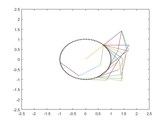
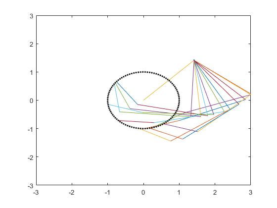
Figure 5: Circular configurations of two CKCs with five links. Left: Ten random circular configurations are depicted for the CKC with link lengths equal to one. Right: Ten random circular configurations are depicted for the CKC with link lengths $2,2,2,1,1$.

Finally, we give examples for CKSs with six links. Figure 6 shows random configurations for CKCs with six links for the orientation vector $\varepsilon^{5}=(\varepsilon_{2},\varepsilon_{3},\varepsilon_{4},\varepsilon_{5})=(0,0,0,0)$.

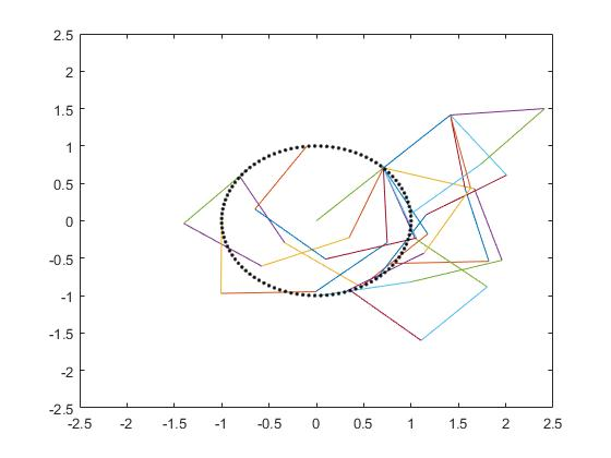
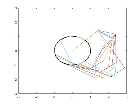
Figure 6: Circular configurations of two CKCs with six links. Left: Ten random circular configurations are depicted for the CKC with link lengths equal to one. Right: Ten random circular configurations are depicted for the CKC with link lengths $2,1,2,1,2,1$.

5 Conclusion and future work

We have developed a new method for computing configurations in terms of joint angles of a CKC by a systematic procedure. Our approach does not require the solution of a system of linear inequalities by linear programming, nor does it rely on probabilistic methods. Numerical examples demonstrate the validity of the proposed work. We expect that the described method can be useful in tasks such as motion planning for CKCs. We anticipate that it will be an interesting approach for future work to further investigate the diagonal space $\mathcal{DS}(a^{n})$. Here it would be interesting to investigate how special designs for CKCs are reflected in the geometry of the diagonal space. Another interesting question is under what conditions $\mathcal{P}(a^{n})\subset\mathcal{Q}(a^{n})$ holds. Since it seems that in this situation $\mathcal{PU}(a^{n})$ and thus $\mathcal{DS}(a^{n})$ can be parameterized using $\Gamma$. A further investigation of $\Gamma$ would then be another interesting line of research.

References

• [1] Suthakorn, J., Chirikjian, G.: A new inverse kinematics algorithm for binary manipulators with many actuators. Adv. Robotics 15 (2), 225-244 (2000). https://doi.org/10.1163/15685530152116245
• [2] Hinokuma, T., Shiga, H.: Topology of the Configuration Space of Polygons as a Codimension One of a Torus. Publ. RIMS, Kyoto Univ. 34 (4), 313-324 (1998). https://doi.org/10.2977/prims/1195144628
• [3] Hausmann, J. C., Knutson, A.: The cohomology ring of polygon spaces. Ann. Inst. Fourier 48 (1), 281-321 (1998). https://doi.org/10.5802/aif.1619
• [4] Cortes J., Simeon, T.:Sampling-based motion planning under kinematic loop closure constraints. In: Algorithmic Foundations of Robotics VI. Springer (2004). https://doi.org/10.1007/10991541_7
• [5] Celaya E., Creemers, T., Ros, L.: Exact interval propagation for the efficient solution of position analysis problems on planar linkages. Mech. Mach. Theory 54, 116-131 (2012). https://doi.org/10.1016/j.mechmachtheory.2012.03.005
• [6] La Valle, S. M., Yakey, J. Kavraki, L.: A probabilistic roadmap approach for systems with closed kinemtic chains. In Proc. IEEE Int. Conf. Robot. Autom. (ICRA) 3, 1671-1676 (1999). https://10.1109/ROBOT.1999.770349
• [7] La Valle, S. M.:Planing Algorithms. Cambridge University Press (2006).
• [8] Han, L., Rudolph, L., Blumenthal, J., Valodzin, I.:Algorithmic Foundation of Robotics VII. Springer, 47, 235-250 (2008).
• [9] Han, L., Rudolph, L.: Inverse Kinematics for a Serial Chain with Joints Under Distance Constraints. Robotics: Science and systems, 177-184 (2006).
• [10] Han, L., Rudolph, L., Blumenthal, J., Valodzin, I.: Convexly stratified deformation spaces and efficient path planning for planar closed chains with revolute joints. Int. J. R. Res. 27, 1189-1212 (2008). https://doi.org/10.1177/0278364908097211
• [11] Milgram, R. J., Trinkle, J. C.: The geometry of configuration spaces for closed chains in two and three dimensions. Homol. Homotopy Appl. 6 (1), 237-267 (2004).
• [12] Milgram, R. J., Trinkle, J. C.: Complete path planning for closed kinematic chains with spherical joints. Int. J. R. Res. 21 (9), 773-789 (2002). https://doi.org/10.1177/0278364902021009119
• [13] Jaillet, L., Porta, J. M.: Path planning under kinematic constraints by rapidly exploring manifolds. IEEE Trans. Robot. 29 (1), 105-117 (2012). https://doi.org/10.1109/TRO.2012.2222272
• [14] Kapovich, M., Millson, J.: On the moduli spaces of polygons in the euclidean plane. J. Differential Geom. 42 (1), 133-164 (1995).
• [15] Liu, G. F., Trinkle, J. C., Milgram, R. J.: Toward complete path planning for planar 3r-manipulators among point obstacles. Algorithmic Foundations of Robotics VI (2004).
• [16] Luenberger D., Yinyu, Y.:Linear and nonlinear programming. Springer, (2004).
• [17] Yakey, J. H., LaValle, S. M., Kavraki, L. E.: Randomized path planning for linkages with closed kinematic chains. IEEE Trans. Robot. Autom. 17 (6), 951-958 (2001). https://doi.org/10.1109/70.976030
• [18] Yajia, Z., Hauser, K., Jingru L.: Robotics and Automation. (ICRA), 2013 IEEE International Conference on (2013).