Linear stability analysis of magnetized relativistic rotating jets

Abstract

We carry out a linear stability analysis of a magnetized relativistic rotating cylindrical jet flow using the approximation of zero thermal pressure. We identify several modes of instability in the jet: Kelvin-Helmholtz, current driven and two kinds of centrifugal-buoyancy modes – toroidal and poloidal. The Kelvin-Helmholtz mode is found at low magnetization and its growth rate depends very weakly on the pitch parameter of the background magnetic field and on rotation. The current driven mode is found at high magnetization, the values of its growth rate and the wavenumber, corresponding to the maximum growth, increase as we decrease the pitch parameter of the background magnetic field. This mode is stabilized by rotation, especially, at high magnetization. The centrifugal-buoyancy modes, arising due to rotation, tend also to be more stable when magnetization is increased. Overall, relativistic jet flows appear to be more stable with respect to their non-relativistic counterpart.

1 Introduction

The study of jet instabilities is of utmost importance for understanding their dynamics and phenomenology. Astrophysical jets propagate over very large distances (up to $10^{9}$ times their initial radius in the case of AGN jets) maintaining a coherent structure and, for this remarkable stability property, an acceptable explanation is still missing. On the other hand, instabilities can play a fundamental role in the dissipation of part of the jet energy, leading to the observed radiation as well as the formation and evolution of various observed structures. One of the mechanisms through which dissipation of the jet energy may occur, and that has recently attracted a lot of interest, is magnetic reconnection (see e.g. Giannios, 2010; Sironi et al., 2015; Werner et al., 2018). In this context, current driven kink instabilities (CDI) may play an important role by enhancing or killing reconnection (Striani et al., 2016; Ripperda et al., 2017a, b). Apart from CDI, other types of instabilities are possible in jets: Kelvin-Helmholtz instabilities (KHI) driven by the velocity shear and centrifugal-buoyancy instabilities driven by the jet rotation. While the Newtonian, or non-relativistic case has been extensively studied, general analyses in the relativistic regime, without invoking the force-free approximation, i.e., taking into account gas inertia, are more limited due to the complexity of the problem. By “relativistic” we mean that the Lorentz factor of the jet flow is larger than unity and/or the magnetization (i.e., the ratio of the magnetic energy density to the energy density of matter) is high, enabling the jet to accelerate to relativistic velocities. KHI have been extensively studied in several different configurations both in the non-relativistic (see e.g. Bodo et al., 1989; Birkinshaw, 1991; Hardee et al., 1992; Bodo et al., 1996; Hardee, 2006; Kim et al., 2015) and relativistic (see e.g. Ferrari et al., 1978; Hardee, 1979; Urpin, 2002; Perucho et al., 2004, 2010; Mizuno et al., 2007) cases. Similarly, CDI have been extensively studied in the Newtonian limit both in the linear (e.g. Appl & Camenzind, 1992; Appl, 1996; Begelman, 1998; Appl et al., 2000; Baty & Keppens, 2002; Bonanno & Urpin, 2011a, b; Das & Begelman, 2018) and nonlinear (e.g., Moll et al., 2008; O’Neill et al., 2012) regimes, while the analysis of the relativistic case has been more limited, most of the linear studies have considered the force-free regime (Voslamber & Callebaut, 1962; Istomin & Pariev, 1994, 1996; Lyubarskii, 1999; Tomimatsu et al., 2001; Narayan et al., 2009; Gourgouliatos et al., 2012; Sobacchi et al., 2017) and the full MHD case has been addressed more recently by Bodo et al. (2013) (hereinafter Paper I), for the cold case, and by Begelman (1998); Kim et al. (2017, 2018), who included thermal pressure. Due to the complexity of the relativistic case, the evolution of CDI beyond the force-free approximation has been tackled often by means of numerical simulations, which mainly focus on the nonlinear behaviour (e.g., Mizuno et al., 2009, 2011; O’Neill et al., 2012; Mizuno et al., 2012; Mignone et al., 2010, 2013; Singh et al., 2016). In the absence of magnetic fields, rotation can drive the centrifugal instability in jets, whose relativistic extension has been recently analysed by Gourgouliatos & Komissarov (2018). The combination of rotation and magnetic field adds another degree of complexity, other kinds of instabilities may arise and the interplay between the different modes can become quite complicated (for non-relativistic studies, see e.g. Kim & Ostriker, 2000; Hanasz et al., 2000; Keppens et al., 2002; Varnière & Tagger, 2002; Huang & Hassam, 2003; Pessah & Psaltis, 2005; Bonanno & Urpin, 2006, 2007; Fu & Lai, 2011). The interplay of rotation and magnetic field, in the non-relativistic case and in the absence of a longitudinal flow, has been analyzed by Bodo et al. (2016) (hereinafter Paper II), and the resulting main, rotationally-induced types of instability – the centrifugal-buoyancy modes – have been identified and described.

In Paper I we considered a cold, relativistic, non-rotating jet and found that KHI is prevalent for matter-dominated jets, while CDI is more effective for magnetically-dominated jets. In Paper II, we considered the effects of rotation in a non-relativistic plasma column, where no longitudinal flow is present. We found additional modes of instability driven by rotation: the centrifugal-buoyancy modes. In this paper, which represents a sequel of Papers I and II, we study the stability problem in the full case of a cold, relativistic, magnetized and rotating jet. We still consider a cold jet, because, on one side, in the case of a Poynting-dominated jet, this can be assumed as a valid approximation and, on the other side, the incorporation of pressure would introduce new kinds of instabilities even more complicating the analysis. This is therefore a further step towards a complete study, where we will drop this limitation in the end. The equilibrium configuration here is similar to that adopted in these papers, which assumes a current distribution that is peaked on the jet axis and closes at very large distances from the jet (i.e., the total net current becomes equal to zero only at large distances). This class of equilibria is different from those considered by Kim et al. (2017, 2018), where the current closes inside the jet. Resulting main modes of the instability in the relativistic and rotating case remain the KH, CD and centrifugal-buoyancy ones. The main goal of the present paper is to investigate the effect of the different parameters of the jet on the growth efficiency of these modes in the more comprehensive relativistic rotating case compared to the relativistic non-rotating and non-relativistic rotating ones analyzed, respectively, in Papers I and II. The main parameters, with respect to which we explore the jet stability, are the Lorentz factor of the propagation velocity along jet axis, pitch of the background magnetic field, degree of magnetization, rotation frequency, vertical/axial wavenumber. In contrast to the present more general study, in Paper I rotation was zero, whereas in Paper II, being in the Newtonian limit, the Lorentz factor was unity and the magnetization, as defined here, was very small. Ultimately, one would like to understand how instabilities can tap part of the jet flow energy, without leading to its disruption. To this aim, numerical simulations are an essential tool, however, linear studies such as the present one may still provide necessary insights.

The plan of the paper is the following: in section 2 we will describe the physical problem, the basic equations, the general equilibrium configuration and the characteristic parameters, in section 3 we present our results, first for the KHI and CDI and then for the centrifugal-buoyancy instabilities and, finally in section 4, we summarize our findings.

2 Problem Description

We investigate the linear stability of a cold (i.e., with zero thermal pressure), magnetized, rotating, relativistic cylindrical flow of an inviscid and infinitely conducting fluid. It is governed by the basic equations of ideal relativistic MHD:

$$\frac{\partial}{\partial t}(\gamma\rho)+\nabla\cdot(\gamma\rho\mn@boldsymbol{v})=0,$$ (1)

$$\gamma\rho\frac{\partial}{\partial t}(\gamma\mn@boldsymbol{v})+\gamma\rho(\mn@boldsymbol{v}\cdot\nabla)(\gamma\mn@boldsymbol{v})=\frac{1}{c}\mn@boldsymbol{J}\times\mn@boldsymbol{B}+\frac{1}{4\pi}(\nabla\cdot\mn@boldsymbol{E})\mn@boldsymbol{E},$$ (2)

$$\frac{1}{c}\frac{\partial\mn@boldsymbol{B}}{\partial t}=-\nabla\times\mn@boldsymbol{E},$$ (3)

$$\frac{1}{c}\frac{\partial\mn@boldsymbol{E}}{\partial t}=\nabla\times\mn@boldsymbol{B}-\frac{4\pi}{c}\mn@boldsymbol{J},$$ (4)

where $\rho$ is the proper density, $\gamma=(1-v^{2}/c^{2})^{-1/2}$ is the Lorentz factor, with $c$ being the speed of light, and $\mn@boldsymbol{v}$, $\mn@boldsymbol{B}$, $\mn@boldsymbol{E}$, $\mn@boldsymbol{J}$ are, respectively, the 3-vectors of the velocity, magnetic field, electric field and current density. These equations are written in the CGS system and a factor of $\sqrt{4\pi}$ is absorbed in the definitions of $\mn@boldsymbol{E}$ and $\mn@boldsymbol{B}$. In the following we choose the units such that the speed of light is unity, $c=1$, .

2.1 Equilibrium Configuration

The equilibrium configuration was described in Paper I, here we summarize the relevant equations. We adopt cylindrical coordinates $(r,\varphi,z)$ (with versors $\mn@boldsymbol{e}_{r},\mn@boldsymbol{e}_{\varphi},\mn@boldsymbol{e}_{z}$) and seek for axisymmetric steady-state solutions (i.e., $\partial_{t}=\partial_{\varphi}=\partial_{z}=0$) of equations (1)-(4). The jet propagates in the vertical/axial ($z$) direction, the magnetic field and velocity have no radial components and consist of a vertical (poloidal), $B_{z},v_{z}$, and toroidal, $B_{\varphi},v_{\varphi}$, components. The magnetic field configuration can be characterized by the pitch parameter

$$P=\frac{rB_{z}}{B_{\varphi}}.$$

The only non-trivial equation is given by the radial component of the momentum equation (2) which, in the zero pressure case, simplifies to

$$\rho\gamma^{2}v_{\varphi}^{2}=\frac{1}{2r}\frac{d(r^{2}H^{2})}{dr}+\frac{r}{2}\frac{dB_{z}^{2}}{dr},$$ (5)

where $H^{2}=B_{\varphi}^{2}-E_{r}^{2}$ (in the non-relativistic case $H^{2}=B_{\varphi}^{2}$) and

$$E_{r}=v_{z}B_{\varphi}-v_{\varphi}B_{z}$$ (6)

Equation (5) leaves the freedom of choosing the radial profiles of all flow variables except one and then solve for the remaining profile. We note that while in the Newtonian case, the presence of a longitudinal velocity has no effect on the radial equilibrium, this no longer holds in the relativistic case, where the Lorentz factor appears in the equilibrium condition (5). The choice of the radial profiles is somewhat arbitrary since we have no direct information about the magnetic configuration in astrophysical jets. We choose to follow the prescriptions given in Papers I and II and to consider a general class of constant density equilibria in which the vertical current density is peaked on the central axis of the jet and is concentrated in a region of the characteristic radius $a$. We prescribe the velocity profile by choosing $\gamma_{z}(r)$, i.e., the Lorentz factor with respect to the $z$-component of the velocity only, of the form

$$\gamma_{z}(r)\equiv\frac{1}{\sqrt{1-v_{z}^{2}}}=1+\frac{\gamma_{c}-1}{\cosh(r/r_{j})^{6}},$$ (7)

where $\gamma_{c}=(1-v_{c}^{2})^{-1/2}$ is the Lorentz factor for the vertical velocity on the central axis, $v_{c}=v_{z}(0)$, and $r_{j}$ is the jet radius. From now on, we will use the subscript $`c`$ to denote values at $r=0$, in addition, all lengths will be expressed in units of $r_{j}$ (recall that the velocities are measured in units of the speed of light $c$). As in Paper I, we prescribe the profile of $H$ as

$$H^{2}=\frac{H^{2}_{c}}{r^{2}}\left[1-\exp\left(-\frac{r^{4}}{a^{4}}\right)\right]$$ (8)

and for the azimuthal velocity we take the form

$$\gamma^{2}v_{\varphi}^{2}=r^{2}\Omega^{2}_{c}\gamma_{c}^{2}\exp\left(-\frac{r^{4}}{a^{4}}\right),$$ (9)

where $\Omega_{c}$ is the angular velocity of the jet rotation on the central axis ($\gamma_{c}\Omega_{c}$ is the angular velocity measured in the jet rest frame). The characteristic radius of the current concentration in the jet is set to $a=0.6$ below. With these choices, from equation (9) we get for $v_{\phi}$ the expression

$$v_{\varphi}^{2}=\frac{r^{2}\gamma_{c}^{2}\Omega_{c}^{2}}{\gamma_{z}^{2}}\left[1+r^{2}\gamma_{c}^{2}\Omega_{c}^{2}\exp\left(-\frac{r^{4}}{a^{4}}\right)\right]^{-1}\exp\left(-\frac{r^{4}}{a^{4}}\right),$$ (10)

from which it is evident that for any value of $\Omega_{c}$, $v_{\phi}$ is always less than unity, i.e., the azimuthal velocity does not exceed the speed of light. From equations (5), (8) and (9), we get the $B_{z}$ profile as

$$B^{2}_{z}=B^{2}_{zc}-(1-\alpha)\frac{H^{2}_{c}\sqrt{\pi}}{a^{2}}{\rm erf}\left(\frac{r^{2}}{a^{2}}\right)$$ (11)

where $\mathrm{erf}$ is the error function and the parameter

$$\alpha=\frac{\rho\gamma_{c}^{2}\Omega^{2}_{c}a^{4}}{2H_{c}^{2}}$$ (12)

measures the strength of rotation: for $\alpha=0$ (no rotation) the gradient of $r^{2}H^{2}$ in equation (5) is exactly balanced by the gradient of $B_{z}^{2}$ ($B_{z}$ decreases outward), whereas for $\alpha=1$, it is exactly balanced by the centrifugal force and $B_{z}$ is constant. Intermediate values of rotation correspond to the range $0<\alpha<1$. As shown in Paper II, one can, in principle, consider also configurations with $\alpha>1$, in which $B_{z}$ grows radially outward, but such configurations will not be considered in the present paper.

The azimuthal field is obtained from the definition of $H$ using the expression of $E_{r}=v_{z}B_{\varphi}-v_{\varphi}B_{z}$. This yields a quadratic equation in $B_{\varphi}$ with the solution

$$B_{\varphi}=\frac{-v_{\varphi}v_{z}B_{z}\mp\sqrt{v_{\varphi}^{2}B_{z}^{2}+H^{2}(1-v_{z}^{2})}}{1-v_{z}^{2}}.$$ (13)

Here we consider the negative branch because it guarantees that $B_{\varphi}$ and $v_{\varphi}$ have opposite signs, as suggested by acceleration models (see e.g., Blandford & Payne, 1982; Ferreira & Pelletier, 1995; Zanni et al., 2007). We choose to characterize the magnetic field configuration by specifying the absolute value of the pitch on the axis, $P_{c}$, and the ratio of the energy density of the matter to the magnetic energy density, $M_{a}^{2}$,

$$P_{c}\equiv\left|\frac{rB_{z}}{B_{\varphi}}\right|_{r=0}\,,\qquad M_{a}^{2}\equiv\frac{\rho\gamma_{c}^{2}}{\left<\mn@boldsymbol{B}^{2}\right>}\,,$$ (14)

where $\left<\mn@boldsymbol{B}^{2}\right>$ represents the radially averaged magnetic energy density across the beam

$$\left<\mn@boldsymbol{B}^{2}\right>=\frac{\int_{0}^{r_{j}}(B_{z}^{2}+B_{\varphi}^{2})r\,dr}{\int_{0}^{r_{j}}r\,dr},$$ (15)

and $r_{j}=1$ in our units. $M_{a}$ is related to the standard magnetization parameter $\sigma=B^{2}/(\rho h)$ ($h$ is the specific enthalpy) used in other studies via $M_{a}^{2}=\gamma_{c}^{2}/\sigma$ and to the relativistic form of the Alfvén speed, $v_{a}=B/\sqrt{\rho h+B^{2}}$, via $M_{a}^{2}=\gamma_{c}^{2}(1-v_{a}^{2})/v_{a}^{2}$ ($c=1$ and in the cold limit $h=1$). The constants $B_{zc}$ and $H_{c}$ appearing in the above equations can be found in terms of $P_{c}$, $M_{a}$ and $\Omega_{c}$ by simultaneously solving equations (14) and (15) using expressions (11) and (13) for the magnetic field components. In particular, from the definition of the pitch parameter, after some algebra, we find (in the $r\rightarrow 0$ limit)

$$a^{4}B^{2}_{zc}=\frac{H_{c}^{2}P_{c}^{2}}{1-\left(P_{c}\Omega_{c}+v_{zc}\right)^{2}}.$$ (16)

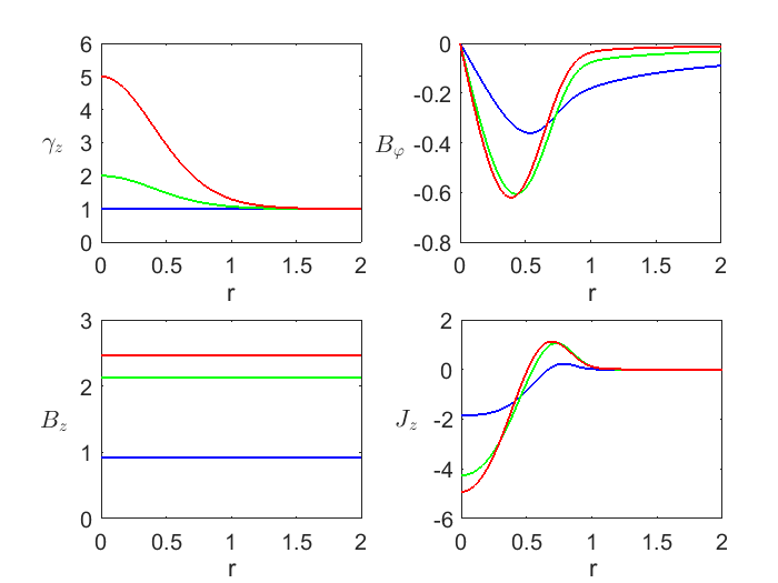
Figure 1: Radial profiles of the Lorentz factor, magnetic field components and axial current density for the equilibrium at $\alpha=1$, $M_{a}^{2}=1$, $P_{c}=1$ and different $\gamma_{c}=1.01~{}(blue),2~{}(green),5~{}(red)$.

Fig. 1 shows the typical radial profile of this equilibrium solution for the special/representative case of maximal rotation, $\alpha=1$, and different $\gamma_{c}$. However, as discussed in Paper II for the non-relativistic case, not all the combinations of $\Omega_{c}$, $\gamma_{c}$, $P_{c}$ and $M_{a}$ are allowed, because, in order to have a physically meaningful solution, we have to impose the additional constraints that $B_{\varphi}^{2}$ and $B_{z}^{2}$ must be everywhere positive. We note that, since $B_{z}^{2}$ decreases with radius monotonically, the condition $\lim_{r\rightarrow\infty}B_{z}^{2}>0$ ensures that $B_{z}^{2}$ is positive everywhere.

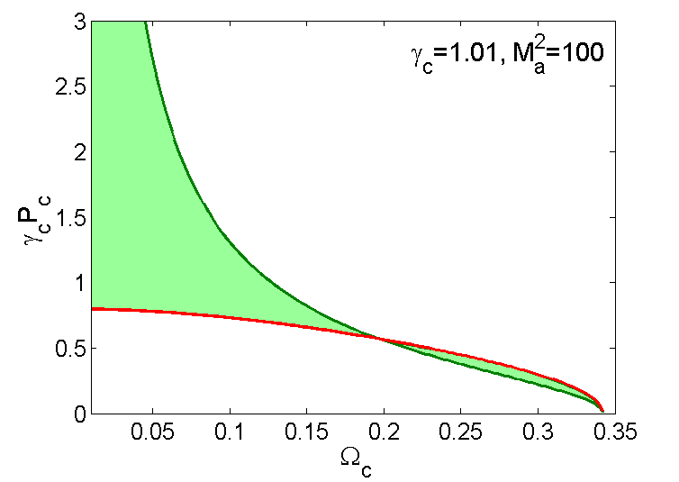
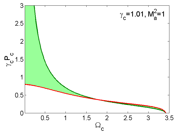
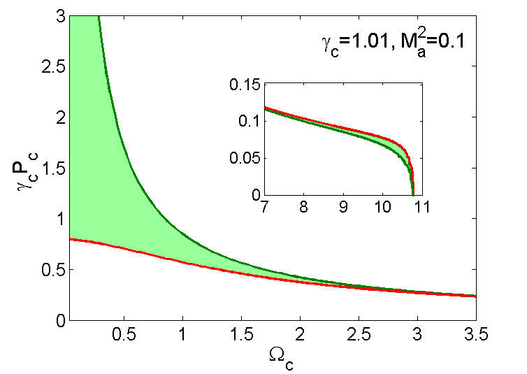
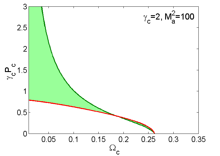
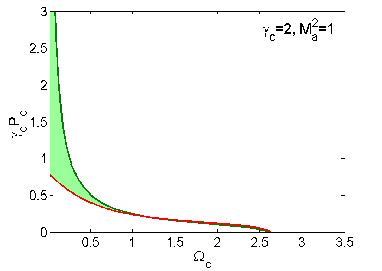
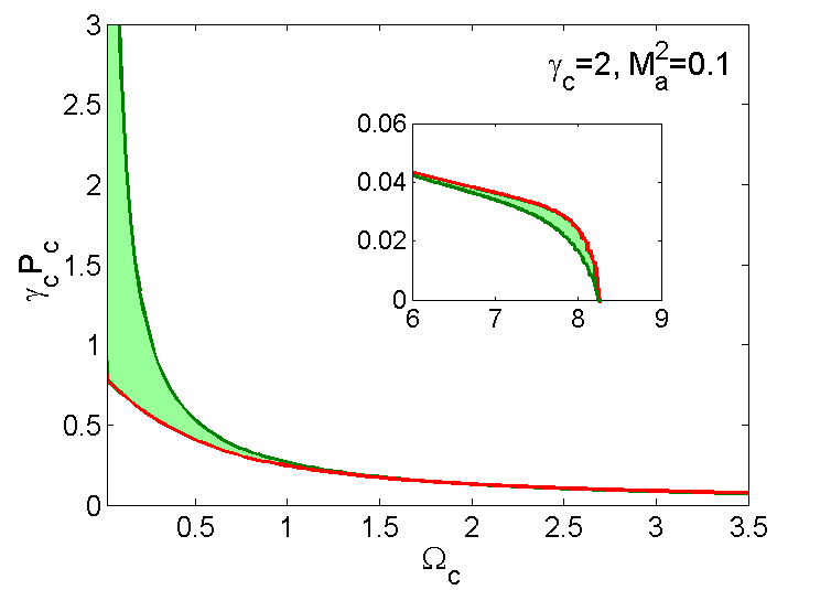
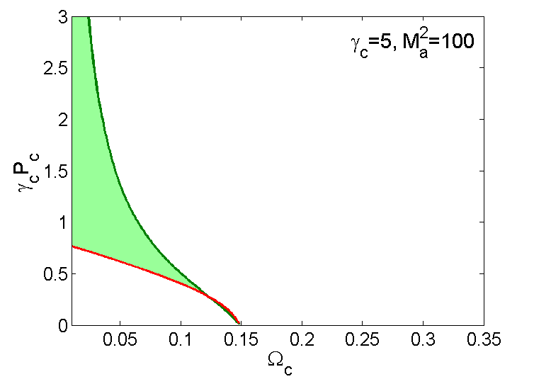
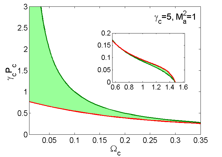
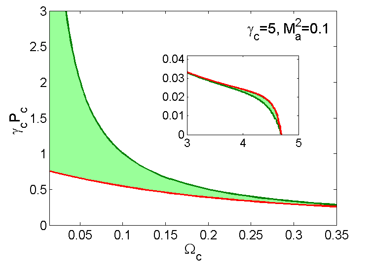
Figure 2: Regions of allowed equilibria in the ($\Omega_{c},\gamma_{c}P_{c}$)-plane shaded in light green. The different panels refer to different values of $\gamma_{c}$ and $M_{a}$, the values corresponding to each panel are reported in the legend. The red curves mark the boundary where $\lim_{r\rightarrow\infty}B_{z}^{2}=0$ and the green curves mark the boundary where $B_{z}^{2}$ is constant with radius ($\alpha=1$). Insets show the maximum $\Omega_{c}$ of the possible equilibria when the latter extend beyond the range of $\Omega_{c}$ represented in these plots.

Fig. 2 shows the allowed region (shaded in light green) in the ($\Omega_{c},\gamma_{c}P_{c}$)-plane, with the red curve marking the boundary where $\lim_{r\rightarrow\infty}B_{z}^{2}=0$ and the green curve marking the boundary where $B_{z}^{2}$ becomes constant with radius (i.e., $\alpha=1$). (As discussed in Paper II, there are also possible equilibria where $B_{z}^{2}$ increases with radius, outside the green curve, but they are not considered here.) We used $\gamma_{c}P_{c}$ on the ordinate axis, since it represents the pitch measured in the jet rest frame. The three panels in each row refer to decreasing values of $M_{a}^{2}$ (from left to right, $M_{a}^{2}=100,1,0.1$) corresponding to increasing strength of the magnetic field, while the three panels in each column refer to increasing value of the Lorentz factor (from top to bottom, $\gamma_{c}=1.01,2,5$). The top leftmost panel with the lowest magnetization and $\gamma_{c}=1.01$ should correspond to the Newtonian limit shown in Fig. 1 of Paper II, comparing these two figures we can see that the shape of the permitted light green regions are nearly the same, while the values of $\Omega_{c}$ are different because of the different normalization, in Paper II it was normalized by $v_{a}/r_{j}$, whereas here it is normalized by $c/r_{j}$. Even at this nearly Newtonian value of $\gamma_{c}=1.01$, the relativistic effects become noticeable starting from intermediate magnetization $M_{a}^{2}=1$ – the corresponding permitted light green region with its green and red boundaries (top middle panel) differs from those in the Newtonian limit $M_{a}^{2}=100$ (top left panel), after taking into account the above normalization of the angular velocity. Generally, in Fig. 2, relativistic effects become increasingly stronger, on one hand, going from left to right, because the Alfvén speed approaches the speed of light, and on the other hand, going from top to bottom, because the jet velocity approaches the speed of light.

At high values of the pitch, there is a maximum allowed value of $\Omega_{c}$, while decreasing the pitch we see that below a threshold value $\gamma_{c}P_{c}=0.8$, the jet must rotate in order to ensure a possible equilibrium and the rotation rate has to increase as the pitch decreases. For low values of $P_{c}$, the allowed range of $\Omega_{c}$ therefore tends to become very narrow. Comparing the panels in the three columns, we see that increasing the magnetic field, the maximum $\Omega_{c}$, found for $P_{c}\rightarrow 0$, increases, scaling with $1/M_{a}$, and the rotation velocities become relativistic. Increasing the value of $\gamma_{c}$ (middle and bottom panels), the allowed values of $\Omega_{c}$ in the laboratory frame (shown in the figure) decrease, however, they increase when measured in the jet rest frame.

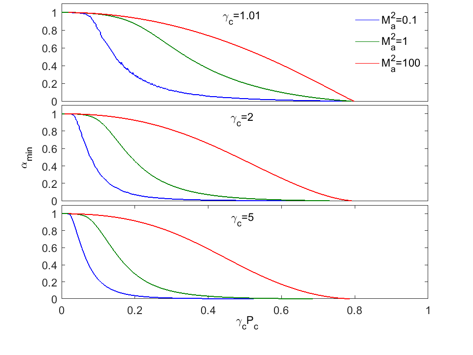
Figure 3: Plots of $\alpha_{min}$ as a function of $\gamma_{c}P_{c}$. $\alpha_{min}$ represents the minimum value of $\alpha$ for which equilibrium is possible. The three panels refer to three different values of $\gamma_{c}$, the corresponding values are reported in each panel. The different curves correspond to different values of $M_{a}$ as indicated in the legend.

Since in the stability analysis we will often make use of the parameter $\alpha$, defined in equation (12), for characterizing the equilibrium solutions, in Fig. 3 we show the minimum value of $\alpha$ required for the existence of the equilibrium as a function of $\gamma_{c}P_{c}$. We recall that $\alpha=0$ corresponds to no rotation and $\alpha=1$ corresponds to the case where $B_{z}$ is constant and the hoop stresses by $B_{\phi}$ are completely balanced by rotation. As discussed above, for $\gamma_{c}P_{c}<0.8$ some rotation is needed for maintaining the equilibrium and this minimum rotation corresponds to $\alpha_{min}$ plotted in Fig. 3. The three panels refer to three different values of $\gamma_{c}$ and in each panel the three curves correspond to three different values of $M_{a}$. Decreasing $\gamma_{c}P_{c}$ below the critical value, $\alpha_{min}$ increases tending to 1 as $\gamma_{c}P_{c}\rightarrow 0$. Comparing the curves for the same value of $\gamma_{c}$ in each panel, we see that $\alpha_{min}$ decreases as $M_{a}$ is decreased. Comparing the different panels, the corresponding curves for the same value of $M_{a}$ also show a decrease of $\alpha_{min}$ with $\gamma_{c}$.

3 Results

In Paper II, we identified and described different linear modes of instability existing in a non-relativistic rotating static (with $v_{z}=0$) column: the CD mode as well as the toroidal and poloidal buoyancy modes driven by the centrifugal force due to rotation. In the present analysis, we have to consider additionally the instabilities driven by the velocity shear between the jet and the ambient medium, that is, KH modes. We will investigate these different perturbation modes in the following subsections.

The small perturbations of velocity and magnetic field about the above-described equilibrium are assumed to have the form $\propto\exp({\rm i}\omega t-{\rm i}m\varphi-{\rm i}kz)$, where the azimuthal (integer) $m$ and axial $k$ wavenumbers are real, while the frequency $\omega$ is generally complex, so that there is instability if its imaginary part is negative, ${\rm Im}(\omega)<0$, and the growth rate of the instability is accordingly given by $-{\rm Im}(\omega)$. The related eigenvalue problem for $\omega$ – the linear differential equations (with respect to the radial coordinate) for the perturbations together with the appropriate boundary conditions in the vicinity of the jet axis, $r\rightarrow 0$, and far from it, $r\rightarrow\infty$ – were formulated in Paper I in a general form for magnetized relativistic rotating jets, but then only the non-rotating case was considered. For reference, in Appendix A, we give the final set of these main equations (22) and (23) with the boundary conditions (24) and (25), which are solved in the present rotating case and the reader can consult Paper I for the details of the derivation. In this study, we focus on $m=1$ modes for the following reasons. For CDI, this kink mode is the most effective one, leading to a helical displacement of the whole jet body, while CDI is absent for $m=-1$ modes (Paper I). As for KHI, it is practically insensitive to the sign of $m$ (Paper I), so we can choose only positive $m$. Finally, as we have seen in Paper II, the centrifugal-buoyancy modes also behave overall similarly at $m=-1$ and $m=1$ for large and small $k$, which are the main areas of these modes’ activity.

Our equilibrium configuration depends on the four parameters $\gamma_{c}$, $\alpha$, $P_{c}$ and $M_{a}$, specifying, respectively, the jet bulk flow velocity along the axis, the strength of the centrifugal force, the magnetic pitch and the magnetization. As mentioned above, relativistic effects become important either at high values of $\gamma_{c}$, because the jet velocity approaches the speed of light, or at low values of $M_{a}$, because the Alfvén speed approaches the speed of light, even when $\gamma_{c}\sim 1$. For some of the parameters we are forced to make a choice of few representative values since it would be impossible to have a full coverage of the four-dimensional parameter space. For $\gamma_{c}$ we choose one value to be $1.01$ since at large $M_{a}$ we make connection with the non-relativistic results (Paper II), while at low $M_{a}$ we can explore the relativistic effects due to the high magnetization. As another value, we choose $\gamma_{c}=10$, which can be considered as representative of AGN jets (Padovani & Urry, 1992; Giovannini et al., 2001; Marscher, 2006; Homan, 2012) (except for some cases in which lower values are used, since the growth rates of the modes for $\gamma_{c}=10$ becomes extremely low). For $\alpha$ we chose the two limiting cases $\alpha=0$ (no rotation) and $\alpha=1$ (centrifugal force exactly balances magnetic forces) and one intermediate value, $\alpha=0.2$, for which the effects due to rotation start to be substantial (notice that the relation between $\alpha$ and the rotation rate is not linear). Finally, for $P_{c}$ we explore several different values, $P_{c}=0.01,\,0.1,\,1,\,10$, depending on the allowed equilibrium configurations (see discussion above).

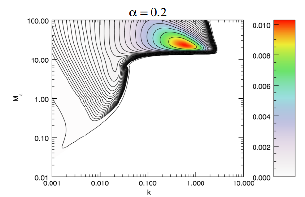
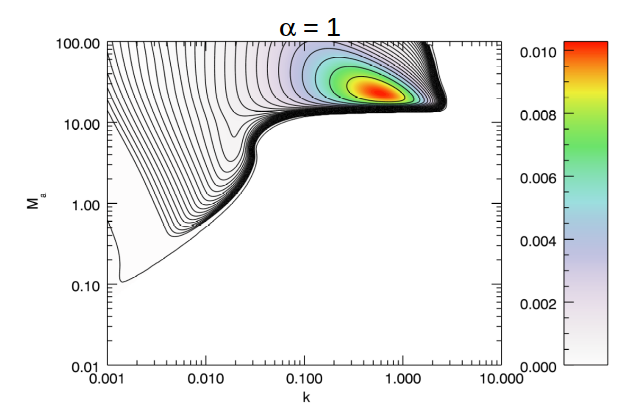
Figure 4: Distribution of the growth rate, $-{\rm Im}(\omega)$, as a function of the wavenumber $k$ and $M_{a}$ for $\gamma_{c}=1.01$ and $P_{c}=10$. The three panels correspond to three different values of $\alpha$ (Top panel: $\alpha=0$; Middle panel: $\alpha=0.2$; Bottom panel: $\alpha=1$). In this and other analogous plots below, the colour scale covers the range from 0 to the maximum value of the growth rate, while the contours are equispaced in logarithmic scale from $10^{-5}$ up to this maximum growth rate.

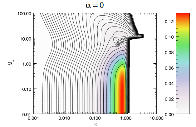
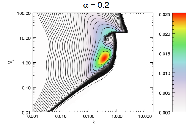
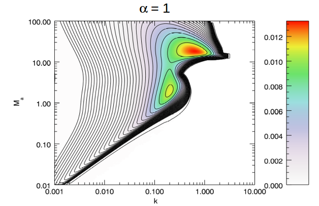
Figure 5: Same as in Fig. 4, but for $\gamma_{c}=1.01$ and $P_{c}=1$.

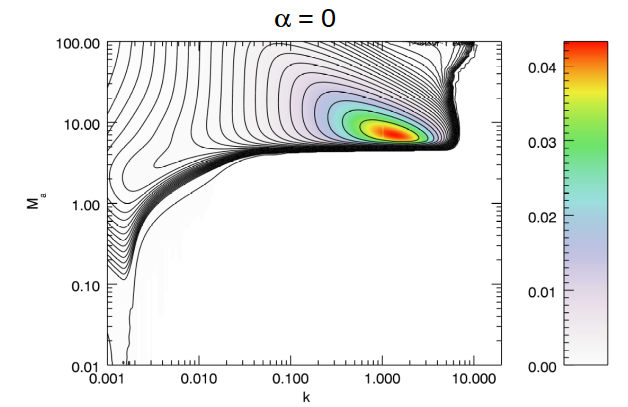
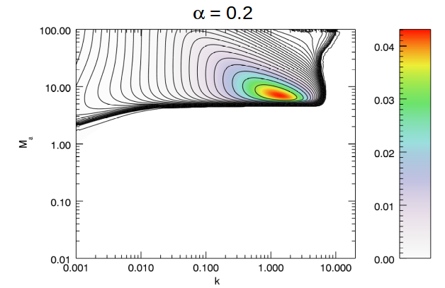
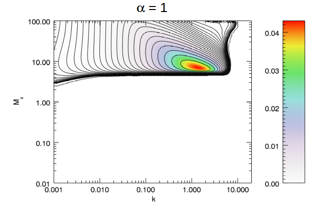
Figure 6: Same as in Fig. 4, but for $\gamma_{c}=10$ and $P_{c}=10$.

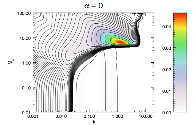
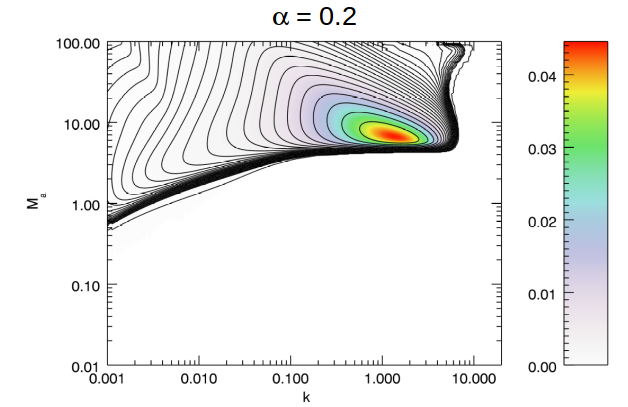
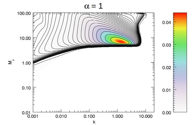
Figure 7: Same as in Fig. 4, but for $\gamma_{c}=10$ and $P_{c}=1$.

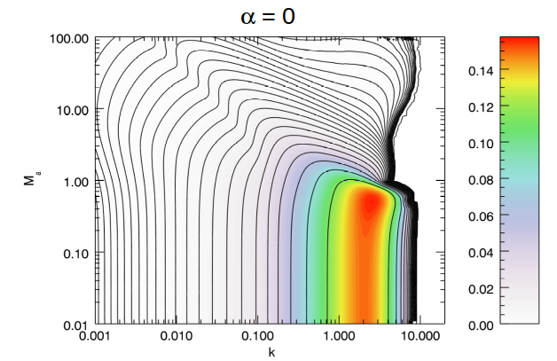
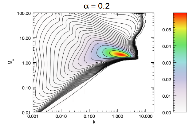
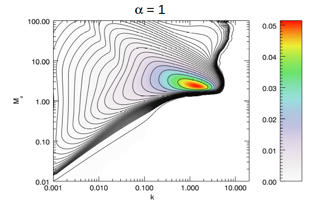
Figure 8: Same as in Fig. 4, but for $\gamma_{c}=10$ and $P_{c}=0.1$.

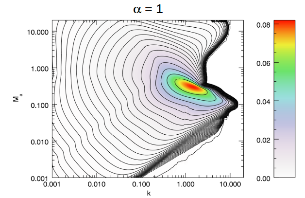
Figure 9: Distribution of the growth rate, $-{\rm Im}(\omega)$, as a function of the wavenumber $k$ and $M_{a}$ for $\gamma_{c}=10$, $\alpha=1$ and $P_{c}=0.01$.

3.1 CD and KH modes

CD and KH modes were already discussed in detail in Paper I, where we found KH modes dominating at large values of $M_{a}$ and CD modes dominating at small values of $M_{a}$. Here we are mainly interested in how they are affected by rotation. In Fig. 4, we show the behaviour of the growth rate (defined as $-{\rm Im}(\omega)$) as a function of the wavenumber $k$ and $M_{a}$ for $P_{c}=10$, $\gamma_{c}=1.01$ and three different values of $\alpha$: $\alpha=0$ in the top panel corresponds to no rotation, $\alpha=1$ in the bottom panel corresponds to the case where rotation exactly balances magnetic forces and as an intermediate value, in the middle panel, we choose $\alpha=0.2$ for which the influence of rotation is already appreciable. The case shown in the top panel is for zero rotation and has already been considered in Paper I, we show it again here in order to highlight the effects of rotation by direct comparison. Increasing rotation (middle and bottom panels), we see a stabilizing effect on CDI, which progressively increases when $M_{a}$ decreases. This stabilizing effect of rotation has been already discussed in Paper II (see also Carey & Sovinec, 2009). In this figure, the difference between the last two values of $\alpha$ may still be small, however, as we will see below, the behaviour can be noticeably different at $M_{a}<1$ for other values of $P_{c}$ and $\gamma_{c}$, especially, in the limit $M_{a}\rightarrow 0$. By contrast, the KH modes, occurring at larger values of $M_{a}$, are essentially unaffected by rotation and, for this value of $P_{c}$, are the dominant modes. Fig. 5 shows the same kind of plots, but for a lower value of the pitch, $P_{c}=1$. In the top panel (no rotation, $\alpha=0$) we see that, as discussed in Paper I, the CD mode increases its growth rate and moves towards larger values of the wavenumber. Rotation has, as before, a stabilizing effect, that becomes stronger as we decrease $M_{a}$. At zero rotation, CDI is the dominant mode, its growth rate is independent from $M_{a}$ (for $M_{a}<1$), and is about an order of magnitude larger than the growth rate of KHI. As we increase rotation, the growth rate of CDI decreases and the stability boundary moves towards smaller and smaller $k$ as $M_{a}$ is decreased. This decrease in the level of CDI in Fig. 5 is most dramatic when $\alpha$ goes from zero to $0.2$ (as it is visible by comparing the top and middle panels), further increasing $\alpha$ to $1$ the decrease is then much less pronounced. As a result, for $\alpha=1$, the KHI is again the mode with the highest growth rate, which, however, has changed only slightly relative to its value in the non-rotating case. The cases with the same high $\gamma_{c}=10$ and three different values of the pitch, $P_{c}=10$, $P_{c}=1$ and $P_{c}=0.1$, are shown, respectively, in Figs. 6, 7 and 8. We note that the pitch measured in the jet rest frame is given by $\gamma_{c}P_{c}$, so these three values would correspond to $P_{c}=100$, $P_{c}=10$ and $P_{c}=1$ when measured in the rest frame. (Additionally, we have to note that for $\gamma_{c}=1.01$ there are no equilibrium solutions for $P_{c}=0.1$.) In the top panel (no rotation) of Fig 6, we therefore see that the stability boundary of the CD modes moves further to the left, i.e., towards smaller wavenumbers compared to the above case with $\gamma_{c}=1.01$, because of the high value of the pitch measured in the jet rest frame. Increasing rotation (middle and bottom panels), below $M_{a}\sim 2$ the CD mode is stable (at least in the wavenumber range considered). For lower values of the pitch in Figs. 7 and 8, in the absence of rotation, the stability limit of the CD modes shifts again to larger $k$ with decreasing pitch. The effect of rotation is thus similar also in this highly relativistic case as it is for $\gamma_{c}=1.01$, being most remarkable when $\alpha$ increases from zero to 0.2. Notice that, as discussed in Paper I, we have a splitting of the CD mode as a function of wavenumber for $P_{c}=1$, this splitting is, however, only present at zero rotation (top panel of Fig. 7). As noted above, the KH mode is essentially unaffected by rotation. Therefore, except for the case with $P_{c}=0.1$ and no rotation, the mode with the highest growth rate remains the KHI. Finally, in Fig. 9 we show the case with $P_{c}=0.01$, $\gamma_{c}=10$ and $\alpha=1$. For this value of $P_{c}$, equilibrium is possible only at high values of $\gamma_{c}$ and the allowed values of $\alpha$ cannot be much smaller than 1. The behavior is similar to those discussed above, on one hand the CDI tends to move towards higher wavenumbers and increase its growth rate due to the decreasing value of $P_{c}$, on the other hand, rotation has the usual stabilizing effect and, as a result, creates an inclined stability boundary that moves towards smaller wavenumbers as $M_{a}$ is decreased.

These results show that the effect of rotation is generally stabilizing for the CD mode, at $M_{a}\lesssim 1$ (high magnetization). An interesting question is then what happens in the limit $M_{a}\rightarrow 0$. This limit, corresponding to the force-free regime in relativistic jets, was investigated by Istomin & Pariev (1994, 1996); Lyubarskii (1999) and Tomimatsu et al. (2001). Tomimatsu et al. (2001) derived the following condition for instability:

$$|B_{\varphi}|>r\Omega_{F}B_{z}$$ (17)

where $\Omega_{F}$ is the angular velocity of field lines that can be expressed as (see Paper I)

$$\Omega_{F}=\frac{v_{\varphi}}{r}-\frac{v_{z}}{P}.$$ (18)

Using equation (6) for the electric field $E_{r}$ and equation (18) for $\Omega_{F}$, the condition (17) can be written as

$$|B_{\varphi}|>|E_{r}|.$$ (19)

The equilibrium condition (5) in the force-free limit becomes

$$\frac{1}{2r}\frac{d(r^{2}H^{2})}{dr}+\frac{r}{2}\frac{dB_{z}^{2}}{dr}=0.$$ (20)

If $B_{z}$ is constant, we have $H=0$ and $|B_{\varphi}|=|E_{r}|$. According to Tomimatsu condition (19), in this case, we are on the stability boundary and the system can be stable. In fact, Istomin & Pariev (1994, 1996) considered such a situation and found stability. On the other hand, if $B_{z}$ decreases radially outward, $H>0$, the Tomimatsu condition is satisfied and there is instability. Lyubarskii (1999) considered such a case and indeed found instability, with a characteristic wavenumber increasing inversely proportional to pitch. In our setup, a constant $B_{z}$ corresponds to $\alpha=1$, while a radially decreasing vertical field corresponds to $\alpha<1$. From the above figures we have seen that, in the presence of rotation, the instability boundary moves towards smaller and smaller values of the wavenumber as $M_{a}$ becomes low. However, it is hard to deduce from this result how exactly the instability region changes along $k$ when approaching the force-free limit, $M_{a}\rightarrow 0$, because of the limited interval of $M_{a}$ and $k$ values represented. Nevertheless, we can see that, in general, at a given small $M_{a}\ll 1$, the stability boundary for $\alpha=1$ tends to be at values of $k$ smaller than those for $\alpha=0.2$ (see e.g., Figs. 5 and 8), that is overall consistent with the results of Istomin & Pariev (1994, 1996); Lyubarskii (1999) and Tomimatsu et al. (2001).

3.2 Centrifugal-buoyancy modes

In Paper II, we demonstrated that in rotating non-relativistic jets, apart from CD and KH modes, there exists yet another important class of unstable modes that are similar to the Parker instability with the driving role of external gravity replaced by the centrifugal force (Huang & Hassam, 2003) and analysed in detail their properties. At small values of $k$, these modes operate by bending mostly toroidal field lines, while at large $k$ they operate by bending poloidal field lines. Accordingly, we labeled them the toroidal and poloidal buoyancy modes (see also Kim & Ostriker, 2000). In this subsection, we investigate how the growth of these modes is affected by relativistic effects.

3.2.1 Toroidal buoyancy mode

The toroidal buoyancy mode operates at small values of $k$ and, in fact, its instability is present only for wavenumbers $k<k_{c}$, where the high wavenumber cutoff $k_{c}$ depends on the pitch parameter and satisfies the condition $k_{c}P_{c}\sim 1$. Fig. 10 presents the typical behaviour of the growth rate of the toroidal mode as a function of $k$ and $M_{a}$ for $P_{c}=1$, $\gamma_{c}=1.01$ and $\alpha=1$. It is seen that in the unstable region, the growth rate is essentially independent from $k$ and reaches a maximum for $M_{a}$ slightly larger than 1. At smaller and larger values of $M_{a}$ the mode is stable or has a very small growth rate, depending on the parameters, as we will see below.

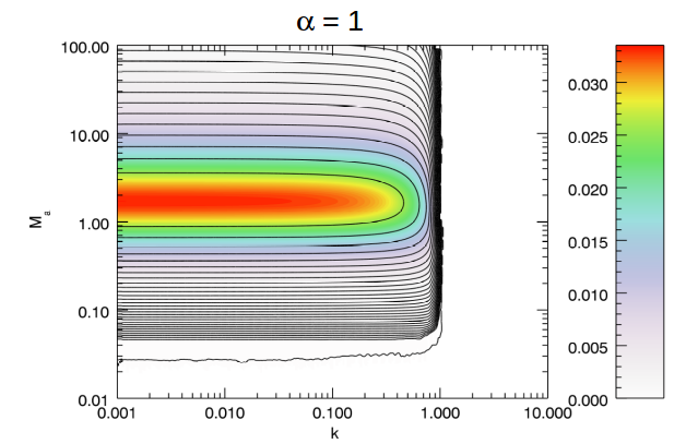
Figure 10: Distribution of the growth rate, $-{\rm Im}(\omega)$, of the toroidal buoyancy mode as a function of the wavenumber $k$ and $M_{a}$ for $\gamma_{c}=1.01$, $\alpha=1$ and $P_{c}=1$.

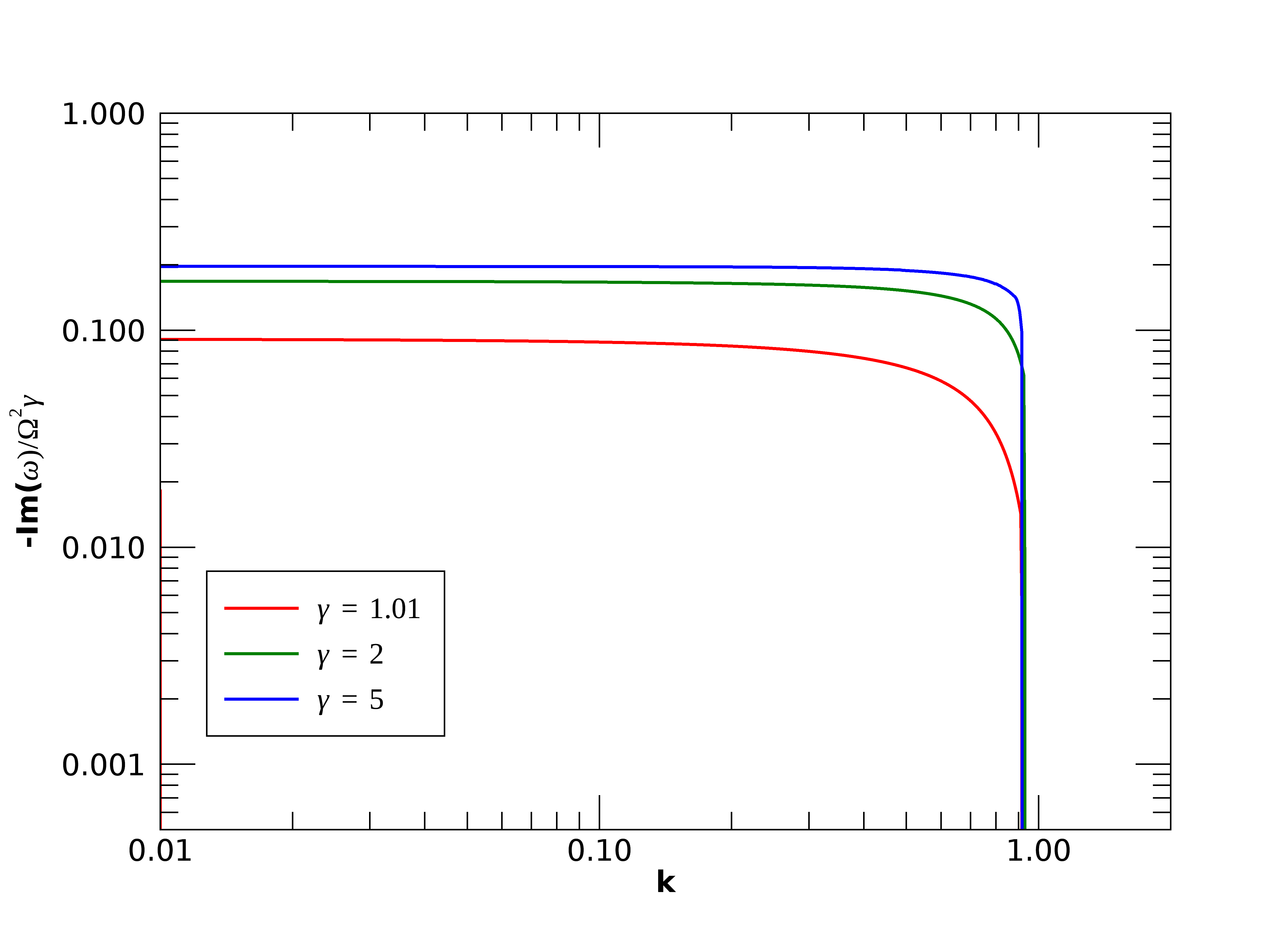
Figure 11: Growth rate of the toroidal mode as a function of $k$ for $\alpha=1$, $P_{c}=1$ and $\gamma_{c}=1.01,2,5$. The growth rate is normalized by $\gamma_{c}\Omega_{c}^{2}$. The three different curves refer to three different values of $\gamma_{c}$ as indicated in the legend. $M_{a}$ is also different for the three curves and for each curve it has the value at which the maximum growth rate is reached at a fixed $k$: $M_{a}=1.5,~{}4.5,~{}15$, respectively, for $\gamma_{c}=1.01,~{}2,~{}5$.

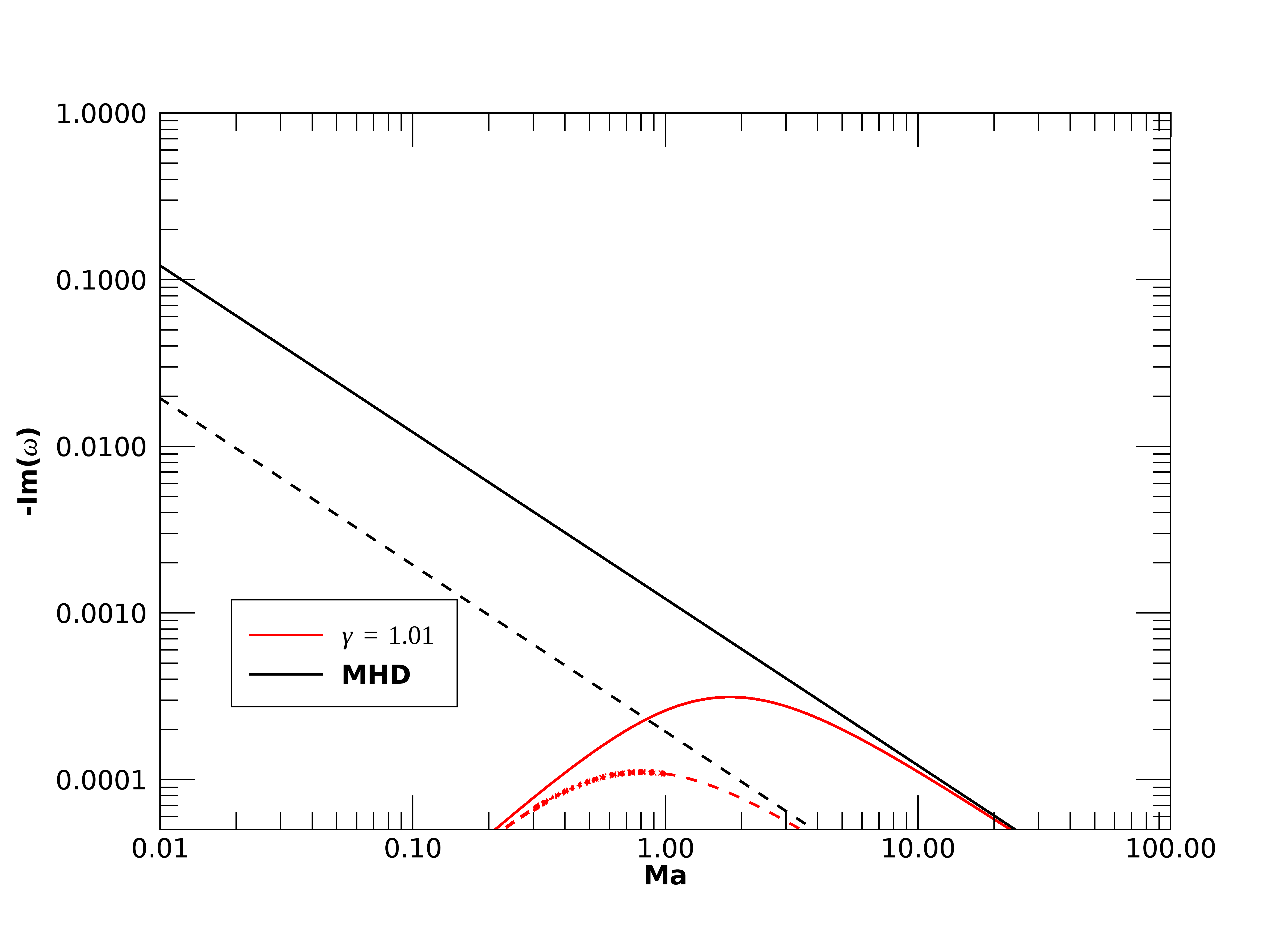
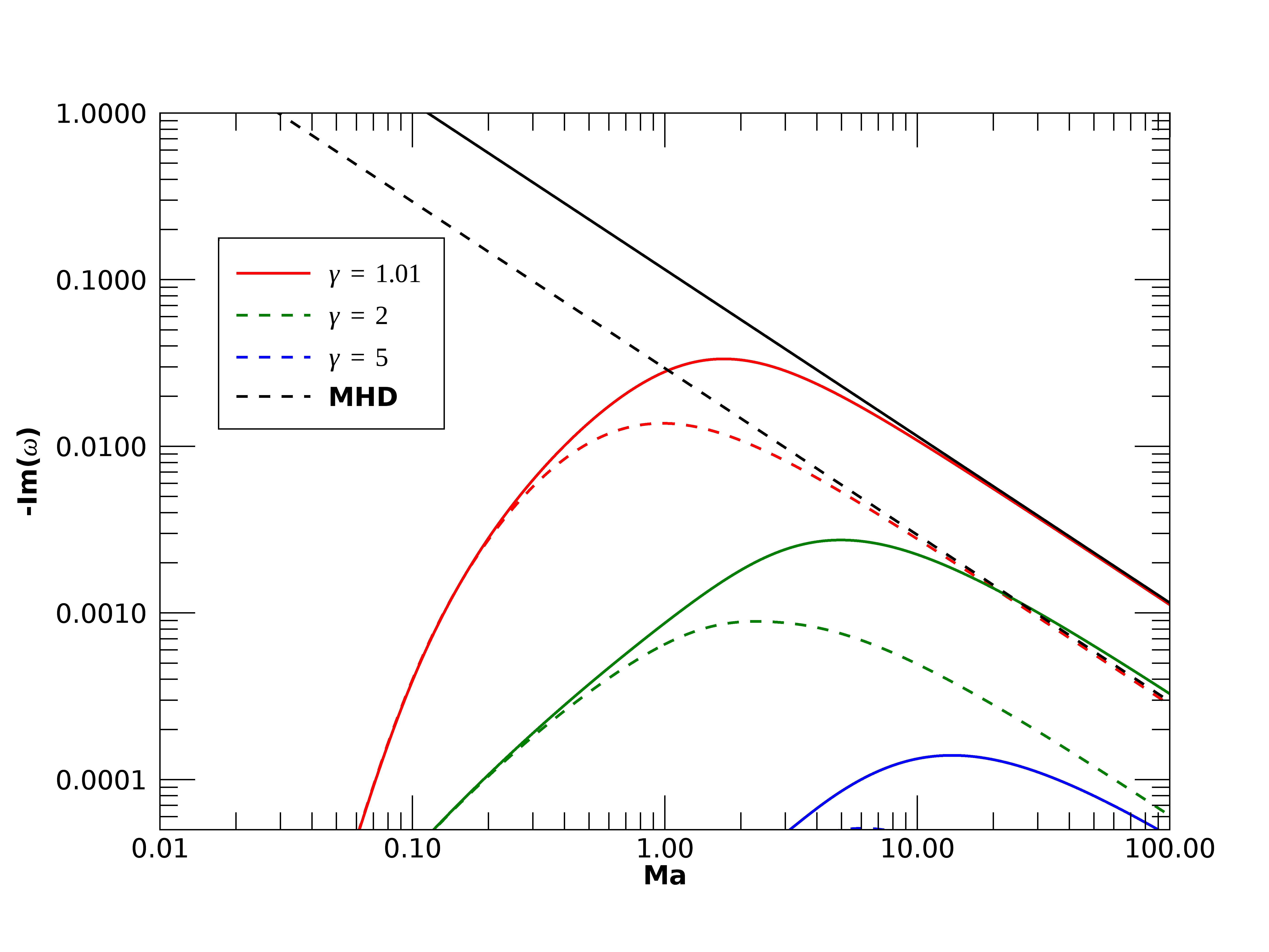
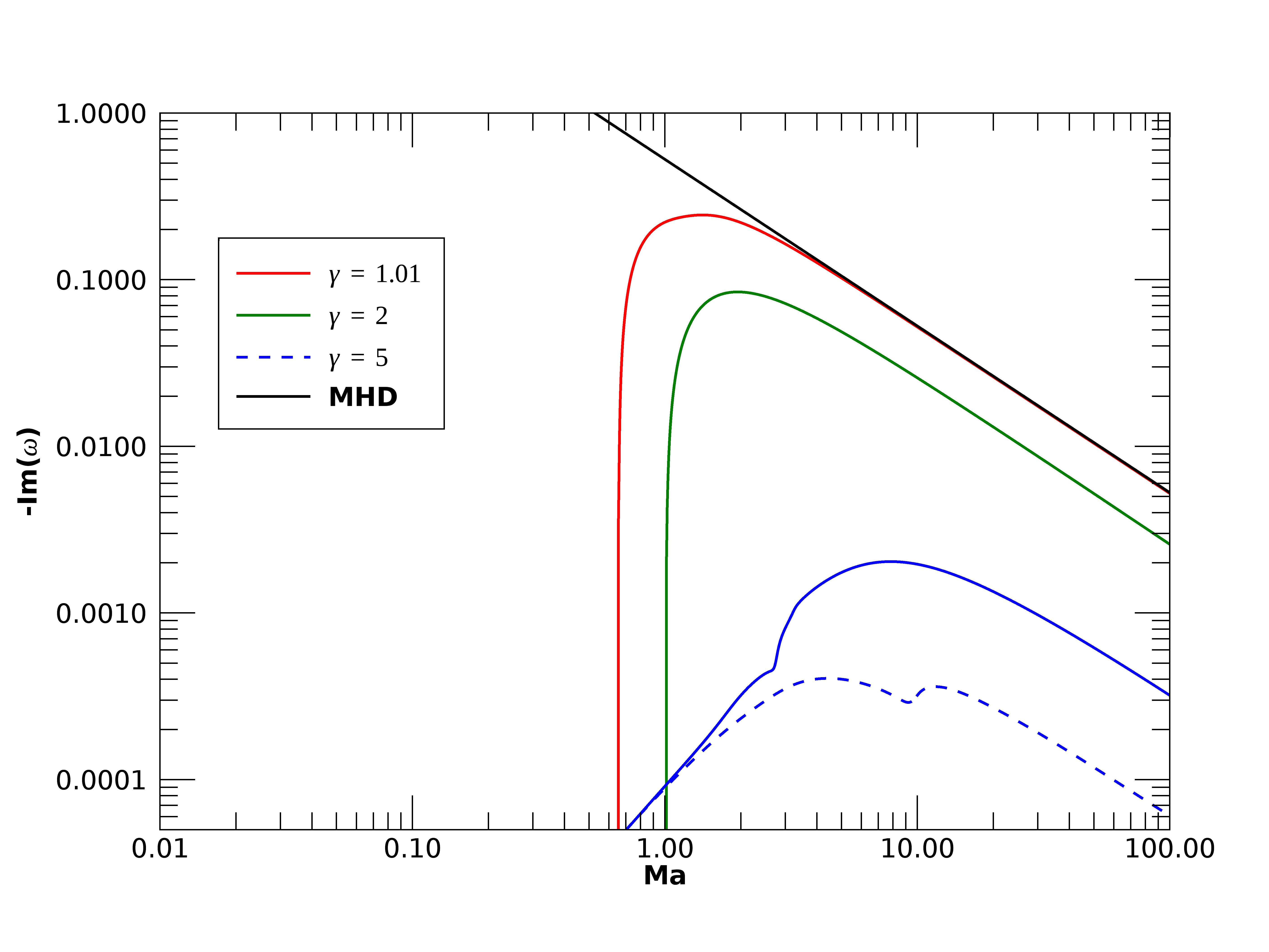
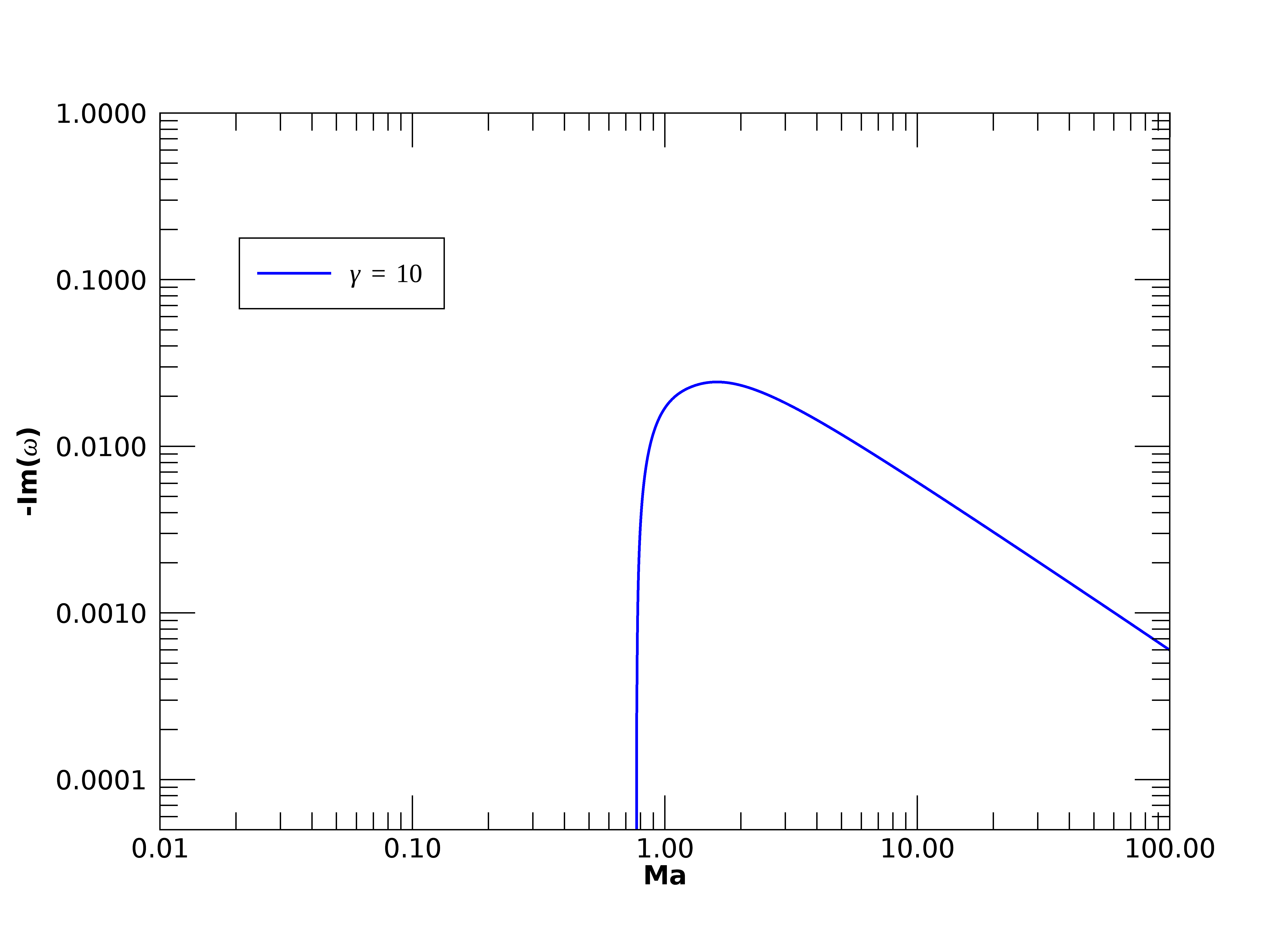
Figure 12: Growth rate of the toroidal mode as a function of $M_{a}$. The four panels refer to different values of the pitch parameter $P_{c}$ (Top left: $P_{c}=10$; Top right: $P_{c}=1$; Bottom left: $P_{c}=0.1$; Bottom right: $P_{c}=0.01$). Solid curves are for $\alpha=1$, dashed curves are for $\alpha=0.2$, curves with different colours refer to different values of $\gamma_{c}=1.01,2,5,10$ as indicated in the legend of each panel. The black lines represent the growth rate calculated with non-relativistic ideal MHD equations at zero thermal pressure and the same pitch and $\alpha$ in the respective panel. If the dashed curve is absent in any panel, this means that the equilibrium with $\alpha=0.2$ is not possible for that pair of $P_{c}$ and $\gamma_{c}$ associated with this panel. The wavenumber is $k=0.01$ in all the cases, although the growth rate is essentially independent of this value.

In Paper II, we showed that the growth rate of the centrifugal-buoyancy modes scales approximately as $\Omega_{c}^{2}$. In the present case, we have to take into account the relativistic effects and, as the mode tends to be concentrated inside the jet, we have to consider quantities measured in the rest frame of the jet. The growth rate in the rest frame should scale as in the non-relativistic case, i.e., as the square of the rotation frequency in this frame. Since the growth rate in the jet rest frame is ${\rm Im}(\omega^{\prime})=\gamma_{c}{\rm Im}(\omega)$, while the rotation frequency is $\Omega^{\prime}_{c}=\gamma_{c}\Omega_{c}$, we can write the scaling law in the lab frame

$$-{\rm Im}(\omega)\sim\gamma_{c}\Omega_{c}^{2},$$ (21)

In Fig. 11, we plot the growth rate normalized according to this scaling, $-{\rm Im}(\omega)/(\gamma_{c}\Omega_{c}^{2})$, as a function of the wavenumber for $\alpha=1$, $P_{c}=1$ and three different values of $\gamma_{c}=1.01,2,5$. For each $\gamma_{c}$, we choose the value of $M_{a}$, which corresponds to the maximum growth rate at a given $k$, these values are reported in the figure caption. For each curve, the value of $\Omega_{c}$ is also different and equal to $0.6$ for $\gamma_{c}=1.01$, $0.09$ for $\gamma_{c}=2$ and $0.01$ for $\gamma_{c}=5$. The growth rate in the unstable range is independent from the wavenumber, as seen in Figs. 10 and 11, and the scaling law (21) reproduces quite well the behaviour of the growth rate at different $\gamma_{c}$: the corresponding curves come close to each other (collapse) when the normalized growth rate is plotted.

To study in more detail the dependence of the toroidal buoyancy instability on the jet flow parameters, in Fig. 12, we plot the growth rate as a function of $M_{a}$ for a given $k$ and various $P_{c}$ and $\gamma_{c}$. Although the value of $k$ is fixed in these plots, we recall that, as we have seen above, there is no dependence of the growth rate on $k$ when $k$ is sufficiently smaller than the cut-off value. So, the curves in this figure would not change for other choices of the unstable wavenumber. The four different panels correspond to different values of the pitch parameter (top left: $P_{c}=10$, top right: $P_{c}=1$, bottom left: $P_{c}=0.1$, bottom right: $P_{c}=0.01$). In each panel, different colours refer to different values of $\gamma_{c}=1.01,2,5,10$, while the solid curves are for $\alpha=1$ and dashed ones for $\alpha=0.2$. Not all curves are present in all panels because, as discussed in subsection 2.1, there are combinations of parameters for which equilibrium is not possible. At large values of $M_{a}\gtrsim 10$ (low magnetization), the growth rate decreases as $1/M_{a}$ for all values of $\gamma_{c}$, $P_{c}$ and $\alpha$ given in these panels. In particular, at $\gamma_{c}=1.01$ the behaviour coincides with the non-relativistic MHD case (black lines in Fig. 12 calculated with ideal non-relativistic MHD equations at zero thermal pressure, as in Paper II). This behaviour can be explained as follows. At large $M_{a}$, rotation is balanced by magnetic forces and hence both decrease with increasing $M_{a}$. As a result, the growth rate of the centrifugal-buoyancy modes decreases too, because it scales with the square of the rotation frequency (Eq. 21). As $M_{a}$ decreases, the growth rate first increases more slowly, reaches a maximum and then decreases at small $M_{a}\ll 1$, as we approach the force-free limit where the centrifugal instabilities should eventually disappear. The behaviour of the growth rate as a function of $\alpha$, $P_{c}$ and $\gamma_{c}$ can be understood from the same scaling with the rotation frequency discussed above. Increasing $\alpha$, the rotation frequency increases as well and, consequently, the growth rate. A decrease in the pitch also leads to an increase of the rotation frequency and, therefore, of the growth rate. Finally, understanding the dependence on $\gamma_{c}$ is more complex since we have to take into account the transformation of all the quantities from the lab frame to the jet frame. The pitch in the jet frame is given by $\gamma_{c}P_{c}$ and is, therefore, larger for larger $\gamma_{c}$ and the rotation rate is consequently smaller. In addition, the growth rate measured in the lab frame is smaller by a factor of $\gamma_{c}$ than the growth rate measured in the jet frame, as a result, the growth rate strongly decreases with $\gamma_{c}$.

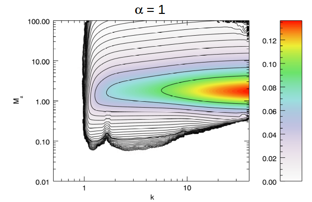
Figure 13: Distribution of the growth rate, $-{\rm Im}(\omega)$, of the poloidal buoyancy mode as a function of the wavenumber $k$ and $M_{a}$ for $\gamma_{c}=1.01$, $\alpha=1$ and $P_{c}=1$.

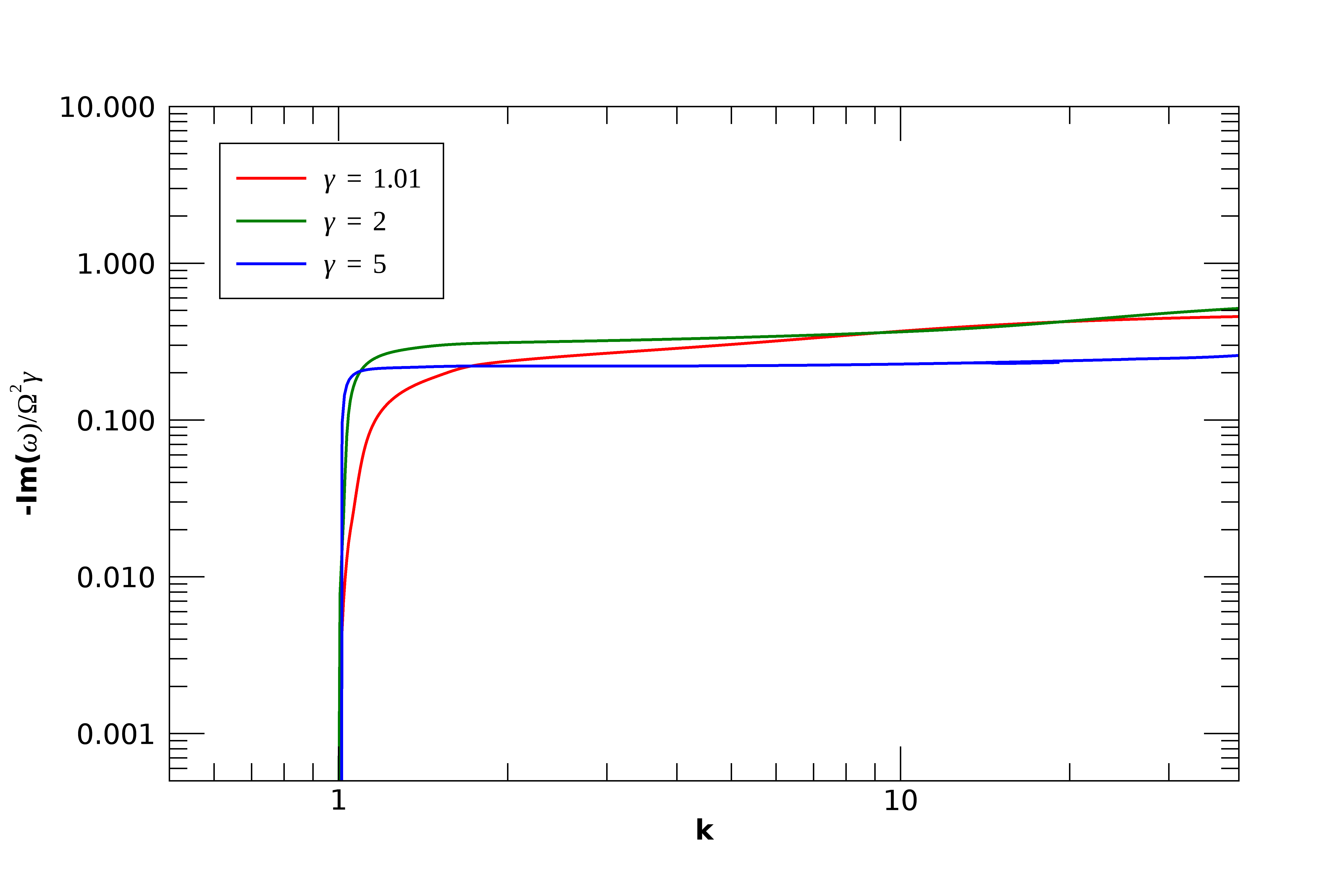
Figure 14: Growth rate of the poloidal buoyancy mode as a function of $k$ for $\alpha=1$, $P=1$ and $\gamma_{c}=1.01,2,5$. The growth rate is normalized by $\gamma_{c}\Omega_{c}^{2}$. The three different curves refer to three different values of $\gamma_{c}$ as indicated in the legend. $M_{a}$ is different for the three curves and for each curve has the value at which the maximum growth rate is found at fixed $k$: $M_{a}=1.8,~{}5.72,~{}14.2$, respectively, for $\gamma_{c}=1.01,~{}2,~{}5$.

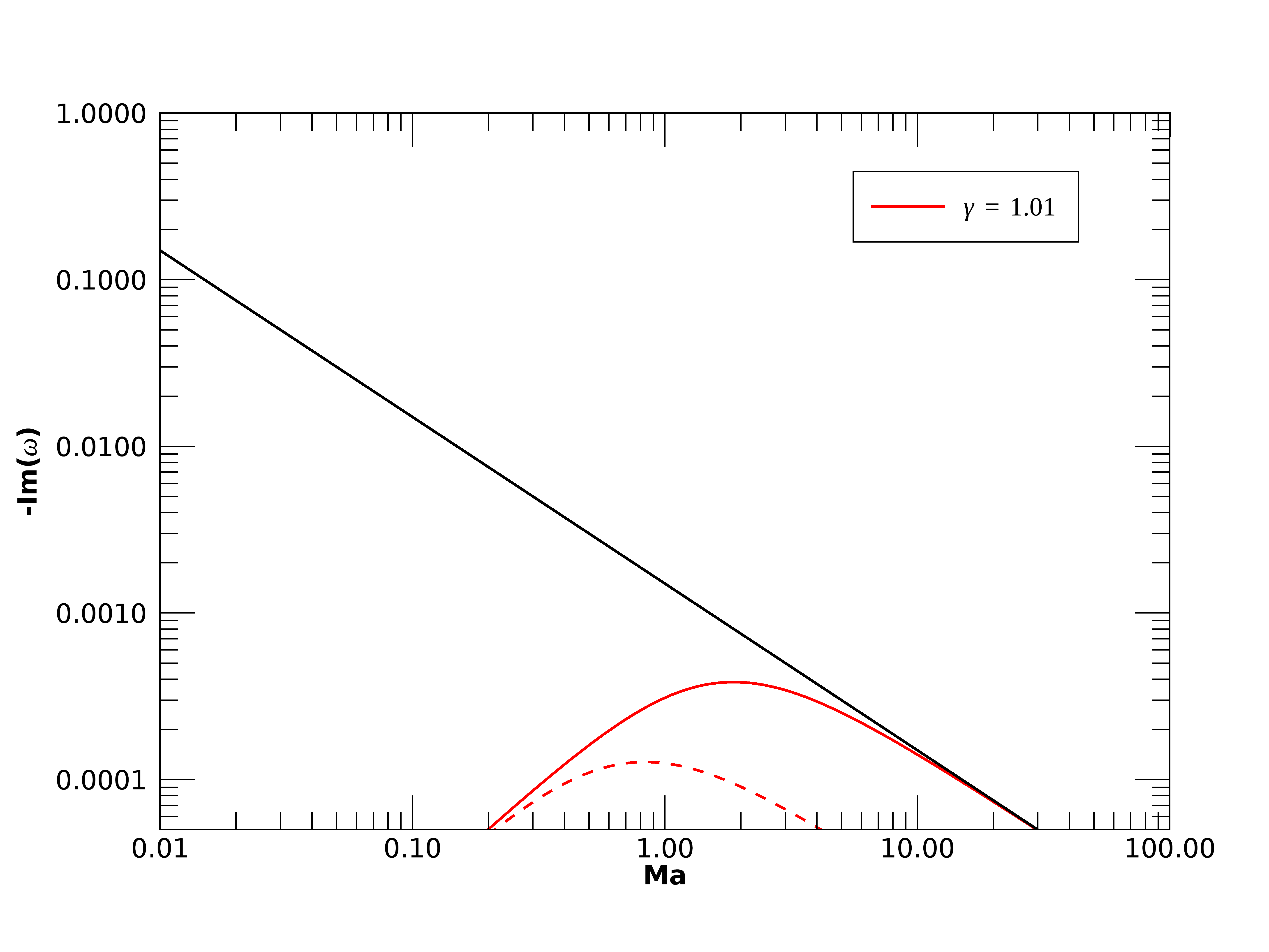
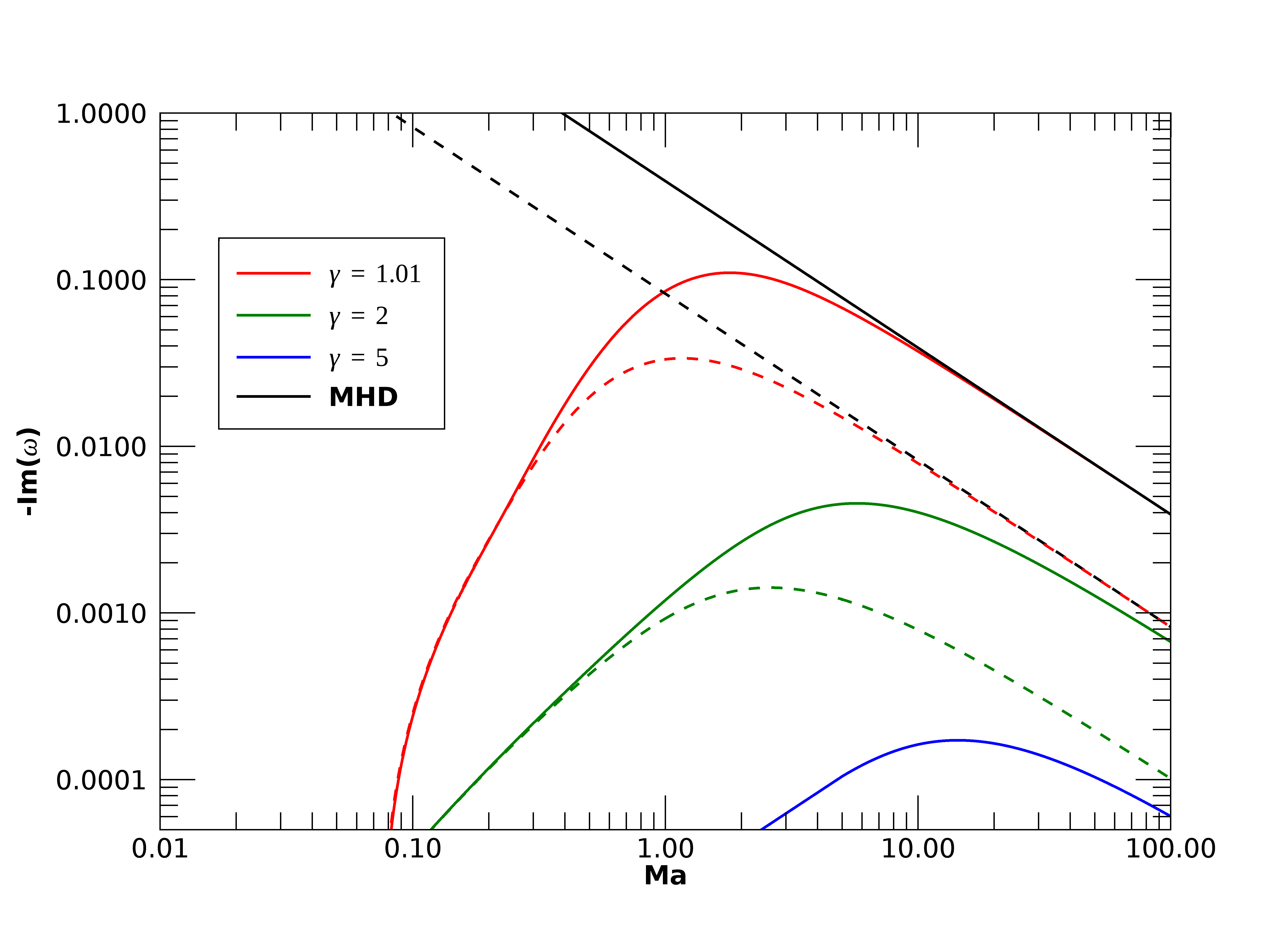
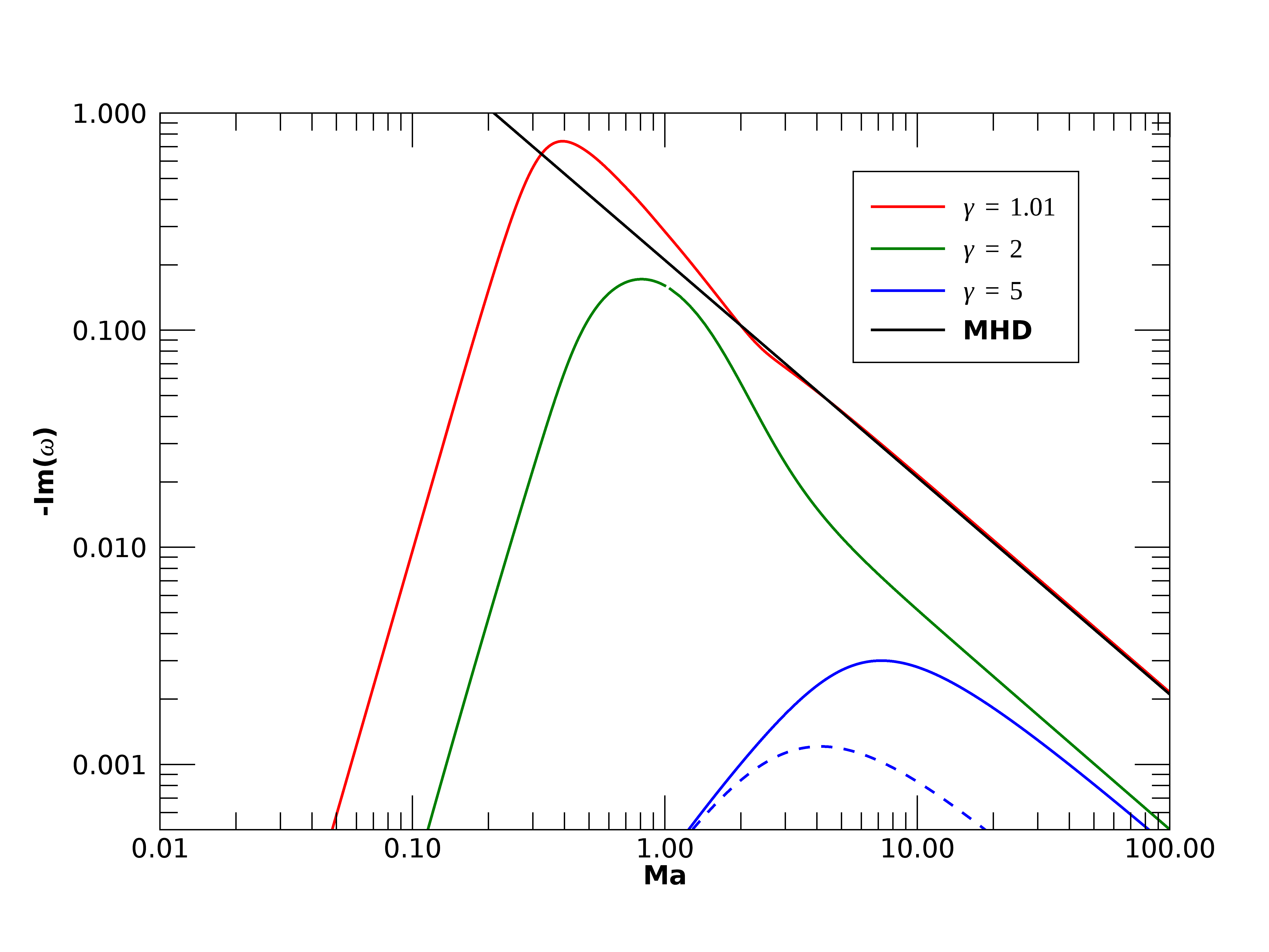
Figure 15: Growth rate of the poloidal buoyancy mode as a function of $M_{a}$. The four panels refer to different values of the pitch parameter $P_{c}$ (Top left: $P_{c}=10$; Top right: $P_{c}=1$; Bottom left: $P_{c}=0.1$; Bottom right: $P_{c}=0.03$). Solid curves are for $\alpha=1$, dashed curves are for $\alpha=0.2$, curves with different colours refer to different values of $\gamma_{c}=1.01,2,5,10$ as indicated in the legend. As in Fig. 12, the black lines represent the results obtained using ideal non-relativistic MHD equations for the same pitch and $\alpha$ in each panel. The dashed curves are absent in those panels with such a pair of $P_{c}$ and $\gamma_{c}$ that do not allow the equilibrium with $\alpha=0.2$. For computation reasons, the wavenumber $k$ is different for each panel (Top left: $k=5$; Top right: $k=10$; Bottom left: $k=14$; Bottom right: $k=40$), but corresponds to the regime where the growth rate practically no longer depends on it.

3.2.2 Poloidal buoyancy mode

Another type of the centrifugal-buoyancy mode existing in the rotating jet is the poloidal buoyancy mode. As mentioned above, this mode operates at large $k$ by bending mostly poloidal field lines. In Fig. 13, we present the behaviour of its growth rate as a function of the wavenumber $k$ and $M_{a}$ for $P_{c}=1$, $\gamma_{c}=1.01$ and $\alpha=1$. This figure is almost specular with respect to Fig. 10 and shows that the poloidal buoyancy instability first starts from the same cutoff wavenumber $k_{c}P_{c}\sim 1$ and extends instead to larger wavenumbers, $k>k_{c}$, having the growth rate somewhat larger than that of the toroidal buoyancy mode. At fixed $k$, it is concentrated in a certain range of $M_{a}$, with the maximum growth rate being achieved around $M_{a}\sim 1$ at every $k$ and decreasing at large and small $M_{a}$. At a given finite $M_{a}$, in the unstable region, the growth rate initially increases with $k$ and then tends to a constant value at $k\gg k_{c}$, as also seen in Fig. 14. Like the toroidal buoyancy mode, the poloidal buoyancy mode obeys the same scaling law (21), because it is also determined by the centrifugal force. This is confirmed by Fig. 14, which presents the growth rate as a function $k$ for $\alpha=1$, $P_{c}=1$ and three different values $\gamma_{c}=1.01,2,5$, while $M_{a}$ is chosen for each curve such that to yield the maximum the growth rate at a given wavenumber. Thus, modification (reduction) of the growth of both centrifugal-buoyancy instabilities in the relativistic case compared to the non-relativistic one is in fact mainly due to the time-dilation effect – in the jet rest frame their growth rate is determined by $\Omega_{c}^{\prime 2}$ in this frame, as it is in the non-relativistic case.

Fig. 15 shows the behaviour of the poloidal buoyancy mode as a function of $M_{a}$ for fixed, sufficiently large values of $k$, when the instability is practically independent of it (see Fig. 14). The values of $\alpha$, $\gamma_{c}$ and $P_{c}$ are the same as used in Fig. 12 except that in the bottom right panel we used $P_{c}=0.03$ instead of 0.01 since for $P_{c}$ slightly below 0.03 the poloidal mode becomes stable, when the cutoff wavenumber, $k_{c}$, which is set by the pitch, becomes larger than the fixed wavenumber ($k=40$) used in this panel. Overall, the dependence of the growth rate of the poloidal buoyancy mode on these parameters is quite similar to that of the toroidal one described above. In particular, at large $M_{a}$ the growth rate varies again as $1/M_{a}$ at all other parameters, coinciding at $\gamma_{c}=1.01$ with the behaviour in the non-relativistic case (black lines). It then increases with decreasing $M_{a}$, reaches a maximum and decreases at small $M_{a}$. The lower is $\gamma_{c}$ the higher is this maximum and the smaller is the corresponding $M_{a}$. On the other hand, with respect to pitch, the highest growth is achieved at $P_{c}\sim 0.1$ at all values of $\gamma_{c}$ considered. Due to the above scaling with the jet rotation frequency, the growth rate also increases with $\alpha$. This behaviour of the poloidal mode instability as a function of $\alpha$, $P_{c}$ and $\gamma_{c}$ can be explained by invoking similar arguments as for the toroidal mode in the previous subsection.

4 Summary

We have investigated the stability properties of a relativistic magnetized rotating cylindrical flow, extending the results obtained in Papers I and II. In Paper I, we neglected rotation, while in Paper II we did not consider the presence of the longitudinal flow and relativistic effects, here we considered the full case, still remaining however in the limit of zero thermal pressure. In the first two papers, we discussed several modes of instabilities that in the present situation all exist. The longitudinal flow velocity gives rise to the KHI, the toroidal component of the magnetic field leads to CDI, while the combination of rotation and magnetic fields gives rise to unstable toroidal and poloidal centrifugal-buoyancy modes. The instability behaviour depends, of course, on the chosen equilibrium configuration and our results can be considered representative of an equilibrium configuration characterized by a distribution of current concentrated in the jet, with the return current assumed to be mainly found at very large distances. Not all combinations of parameters are allowed: there are combinations for which equilibrium solution does not exist. More precisely, for any given rotation rate, there is a minimum value of the pitch, below which no equilibrium is possible. Increasing the rotation rate, this minimum value of the pitch decreases.

The behaviour of KHI and CDI is similar to that discussed in Paper I, at high values of $M_{a}$ we find the KHI, while at low values we find the CDI. The KHI is largely unaffected by rotation, which, on the contrary, has a strong stabilizing effect on the CDI. Decreasing $M_{a}$ and increasing rotation, the unstable region (stability boundary) progressively moves towards smaller axial wavenumbers. A decreasing value of the pitch, on the other hand, moves the stability limits towards larger axial wavenumbers. For relativistic flows, we have also to take into account that the pitch measured in the jet rest frame, which determines the behaviour of the CDI, is $\gamma_{c}$ times the value measured in the laboratory frame, therefore relativistic flows, with the same pitch, are more stable. In Paper I, we found a scaling law showing that the growth rate of CDI strongly decreases with $\gamma_{c}$, while an even stronger stabilization effect is found here due to the combination of relativistic effects and rotation. Extrapolating the behaviour found at low values of $M_{a}$ to the limit $M_{a}\rightarrow 0$, the results are in agreement with Tomimatsu condition (Tomimatsu et al., 2001), applicable to the force-free limit.

Rotation drives centrifugal-buoyancy modes: the toroidal buoyancy mode at low wavenumbers and the poloidal buoyancy mode at high axial wavenumbers. Apart from the different range of these wavenumbers, they have a similar behaviour and their growth rate scales with the square of the rotation frequency, which, in turn, increases as the pitch decreases; therefore they become important at low values of the pitch. In the unstable range, the growth rate is independent from the wavenumber. As the magnetic field increases they tend to be more stable. The same happens increasing the Lorentz factor of the flow.

In this paper, we have considered only the $m=1$ mode, as this mode is thought to be the most dangerous one for jets. Higher order modes $(m>1)$ can trigger instabilities internally in the jet, instead of a global kink. These perturbations can cause inherent breakup of current sheets, reconnection, etc. So, these modes are also interesting to study in the future. If the global jet can remain stable for long time scales and large distances, locally, higher order modes can cause local instabilities that can or cannot disrupt the jet.

In summary, rotation has a stabilizing effect on the CDI which becomes more and more efficient as the magnetization is increased. Rotation on the other hand drives centrifugal modes, which, however, are also stabilized at high magnetizations. Finally, relativistic jet flows tend to be more stable compared to their non-relativistic counterparts.

Appendix A Equations of the eigenvalue problem for the jet stability

Considering small perturbations of the velocity, electric and magnetic fields, $\mn@boldsymbol{v}_{1}$, $\mn@boldsymbol{E}_{1}$, $\mn@boldsymbol{B}_{1}\propto\exp({\rm i}\omega t-{\rm i}m\varphi-{\rm i}kz)$, about the equilibrium state with $\mn@boldsymbol{v}=(0,v_{\varphi},v_{z})$, $\mn@boldsymbol{E}=(E_{r},0,0)$, $\mn@boldsymbol{B}=(0,B_{\varphi},B_{z})$ described in subsection 2.1, and linearizing the main equations (1)-(4), after some algebra, we arrive at the following system of linear differential equations for the radial displacement $\xi_{1r}=-{\rm i}v_{1r}/\tilde{\omega}$ and electromagnetic pressure $\Pi_{1}=\mn@boldsymbol{B}\cdot\mn@boldsymbol{B}_{1}-\mn@boldsymbol{E}\cdot\mn@boldsymbol{E}_{1}=B_{\varphi}B_{1\varphi}+B_{z}B_{1z}-E_{r}E_{1r}$ (see Appendix A of Paper I for the detailed derivations),

$$\left.D\frac{d\xi_{1r}}{dr}=\left(C_{1}+\frac{C_{2}-Dk_{B}^{\prime}}{k_{B}}-\frac{D}{r}\right)\xi_{1r}-C_{3}\Pi_{1}\right.$$ (22)

$$D\frac{d\Pi_{1}}{dr}=\left[A_{1}D-\frac{\rho\gamma^{2}v_{\varphi}^{2}}{r}\left(C_{1}+\frac{C_{2}-Dk^{\prime}_{B}}{k_{B}}\right)+\frac{C_{4}}{r}+C_{5}\right]\xi_{1r}+\left[\frac{1}{r}\left(\rho\gamma^{2}v_{\varphi}^{2}C_{3}-2D+C_{6}\right)+C_{7}\right]\Pi_{1},$$ (23)

where

$$D\equiv\left(\frac{B^{2}}{\rho\gamma^{2}}+1\right)B^{2}\tilde{\omega}^{2}+\frac{k_{B}B^{2}}{\rho\gamma^{2}}\left[2\tilde{\omega}(\mn@boldsymbol{v}\cdot\mn@boldsymbol{B})-\frac{k_{B}}{\gamma^{2}}\right],$$

$$\tilde{\omega}\equiv\omega-\frac{m}{r}v_{\varphi}-kv_{z},\qquad k_{B}\equiv\frac{m}{r}B_{\varphi}+kB_{z},\qquad k_{B}^{\prime}\equiv\frac{dk_{B}}{dr},\qquad B^{2}=B_{\varphi}^{2}+B_{z}^{2}.$$

The other quantities, $A_{1},C_{1},C_{2},C_{3},C_{4},C_{5},C_{6},C_{7}$ contained in these equations, also depend on the chosen profile of the equilibrium solution, and their explicit forms are derived in Appendix B of Paper I. They are rather long expressions and we do not give them here.

The boundary conditions near the jet axis and at large radii are also derived in Appendix C and D of Paper I and are as follows. In the vicinity of the jet axis, $r\rightarrow 0$, the regular solutions have the form $\xi_{1r}\propto r^{|m|-1},\Pi_{1}\propto r^{|m|}$ $(|m|\geq 1)$ and their ratio is

$$\frac{\Pi_{1}}{\xi_{1r}}=\frac{r\rho\gamma_{c}^{2}}{mB_{c}^{2}}\left[{\rm sign}(m)D+2B_{z}^{2}\left(\tilde{\omega}v^{\prime}_{\varphi}+\frac{B^{2}}{\rho\gamma^{2}}\left(\omega-m\Omega_{F}\right)\Omega_{F}+\frac{B^{2}B^{\prime}_{\varphi}k_{B}}{\rho\gamma^{2}B_{z}^{2}}\right)\right]_{|r=0}.$$ (24)

Here $\Omega_{F}$ is the angular velocity of magnetic field lines given by equation (18).

At large radii, $r\rightarrow\infty$, the solution represents radially propagating waves that vanish at infinity. The electromagnetic pressure perturbation of these waves is given by the Hankel function of the first kind, $\Pi_{1}=H^{(1)}_{\nu}(\chi r)$, where

$$\chi^{2}=\frac{\rho+B_{z}^{2}}{B_{z}^{2}}\omega^{2}-k^{2},~{}~{}~{}~{}\nu^{2}=m^{2}+\frac{\rho B_{\varphi c}^{2}\omega^{2}}{B_{z}^{4}},$$

with the leading term of the asymptotic expansion at $r\rightarrow\infty$

$$\Pi_{1}=H_{\nu}^{(1)}(\chi r)\simeq\sqrt{\frac{2}{\pi\chi r}}\exp{\left[{\rm i}\left(\chi r-\frac{\nu\pi}{2}-\frac{\pi}{4}\right)\right]}.$$ (25)

In this expression, the complex parameter $\chi$ can have either positive or negative sign,

$$\chi=\pm\sqrt{\frac{\rho+B_{z}^{2}}{B_{z}^{2}}\omega^{2}-k^{2}}.$$ (26)

Requiring that the perturbations decay at large radii, in equation (26), we choose the root that has a positive imaginary part, ${\rm Im}(\chi)>0$. These perturbations are produced within the jet and hence at large radii should have the character of radially outgoing waves. This implies that the real parts of $\chi$ and $\omega$ should have opposite signs, ${\rm Re}(\omega){\rm Re}(\chi)<0$ (Sommerfeld condition), in order to give the phase velocity directed outwards from the jet. As a result, the asymptotic behaviour of the displacement $\xi_{1r}$ can be readily obtained from $\Pi_{1}$ correct to $O(r^{-3})$

$$\xi_{1r}=\frac{\Pi_{1}}{\omega^{2}(\rho+B^{2})-k_{B}^{2}}\left({\rm i}\chi-\frac{1}{2r}\right).$$

The main equations (22) and (23) together with the above boundary conditions at small (24) and large (25) radii are solved via shooting method to find the eigenvalues of $\omega$.

References

- Appl (1996) Appl S., 1996, A&A, 314, 995
- Appl & Camenzind (1992) Appl S., Camenzind M., 1992, A&A, 256, 354
- Appl et al. (2000) Appl S., Lery T., Baty H., 2000, A&A, 355, 818
- Baty & Keppens (2002) Baty H., Keppens R., 2002, ApJ, 580, 800
- Begelman (1998) Begelman M. C., 1998, ApJ, 493, 291
- Birkinshaw (1991) Birkinshaw M., 1991, The stability of jets. p. 278
- Blandford & Payne (1982) Blandford R. D., Payne D. G., 1982, MNRAS, 199, 883
- Bodo et al. (2013) Bodo G., Mamatsashvili G., Rossi P., Mignone A., 2013, MNRAS, 434, 3030
- Bodo et al. (2016) Bodo G., Mamatsashvili G., Rossi P., Mignone A., 2016, MNRAS, 462, 3031
- Bodo et al. (1989) Bodo G., Rosner R., Ferrari A., Knobloch E., 1989, ApJ, 341, 631
- Bodo et al. (1996) Bodo G., Rosner R., Ferrari A., Knobloch E., 1996, ApJ, 470, 797
- Bonanno & Urpin (2006) Bonanno A., Urpin V., 2006, Phys. Rev. E, 73, 066301
- Bonanno & Urpin (2007) Bonanno A., Urpin V., 2007, ApJ, 662, 851
- Bonanno & Urpin (2011a) Bonanno A., Urpin V., 2011a, Phys. Rev. E, 84, 056310
- Bonanno & Urpin (2011b) Bonanno A., Urpin V., 2011b, A&A, 525, A100
- Carey & Sovinec (2009) Carey C. S., Sovinec C. R., 2009, ApJ, 699, 362
- Das & Begelman (2018) Das U., Begelman M. C., 2018, ArXiv e-prints:1807.11480
- Ferrari et al. (1978) Ferrari A., Trussoni E., Zaninetti L., 1978, A&A, 64, 43
- Ferreira & Pelletier (1995) Ferreira J., Pelletier G., 1995, A&A, 295, 807
- Fu & Lai (2011) Fu W., Lai D., 2011, MNRAS, 410, 399
- Giannios (2010) Giannios D., 2010, MNRAS, 408, L46
- Giovannini et al. (2001) Giovannini G., Cotton W. D., Feretti L., Lara L., Venturi T., 2001, ApJ, 552, 508
- Gourgouliatos et al. (2012) Gourgouliatos K. N., Fendt C., Clausen-Brown E., Lyutikov M., 2012, MNRAS, 419, 3048
- Gourgouliatos & Komissarov (2018) Gourgouliatos K. N., Komissarov S. S., 2018, MNRAS, 475, L125
- Hanasz et al. (2000) Hanasz M., Sol H., Sauty C., 2000, MNRAS, 316, 494
- Hardee (1979) Hardee P. E., 1979, ApJ, 234, 47
- Hardee (2006) Hardee P. E., 2006, in P. A. Hughes & J. N. Bregman ed., Relativistic Jets: The Common Physics of AGN, Microquasars, and Gamma-Ray Bursts Vol. 856 of American Institute of Physics Conference Series, AGN Jets: A Review of Stability and Structure. pp 57–77
- Hardee et al. (1992) Hardee P. E., Cooper M. A., Norman M. L., Stone J. M., 1992, ApJ, 399, 478
- Homan (2012) Homan D. C., 2012, in International Journal of Modern Physics Conference Series Vol. 8 of International Journal of Modern Physics Conference Series, Physical Properties of Jets in AGN. pp 163–171
- Huang & Hassam (2003) Huang Y.-M., Hassam A. B., 2003, Physics of Plasmas, 10, 204
- Istomin & Pariev (1994) Istomin Y. N., Pariev V. I., 1994, MNRAS, 267, 629
- Istomin & Pariev (1996) Istomin Y. N., Pariev V. I., 1996, MNRAS, 281, 1
- Keppens et al. (2002) Keppens R., Casse F., Goedbloed J. P., 2002, ApJ, 569, L121
- Kim et al. (2017) Kim J., Balsara D. S., Lyutikov M., Komissarov S. S., 2017, MNRAS, 467, 4647
- Kim et al. (2018) Kim J., Balsara D. S., Lyutikov M., Komissarov S. S., 2018, MNRAS, 474, 3954
- Kim et al. (2015) Kim J., Balsara D. S., Lyutikov M., Komissarov S. S., George D., Siddireddy P. K., 2015, MNRAS, 450, 982
- Kim & Ostriker (2000) Kim W.-T., Ostriker E. C., 2000, ApJ, 540, 372
- Lyubarskii (1999) Lyubarskii Y. E., 1999, MNRAS, 308, 1006
- Marscher (2006) Marscher A. P., 2006, in Hughes P. A., Bregman J. N., eds, Relativistic Jets: The Common Physics of AGN, Microquasars, and Gamma-Ray Bursts Vol. 856 of American Institute of Physics Conference Series, Relativistic Jets in Active Galactic Nuclei. pp 1–22
- Mignone et al. (2010) Mignone A., Rossi P., Bodo G., Ferrari A., Massaglia S., 2010, MNRAS, 402, 7
- Mignone et al. (2013) Mignone A., Striani E., Tavani M., Ferrari A., 2013, MNRAS, 436, 1102
- Mizuno et al. (2007) Mizuno Y., Hardee P., Nishikawa K.-I., 2007, ApJ, 662, 835
- Mizuno et al. (2009) Mizuno Y., Lyubarsky Y., Nishikawa K.-I., Hardee P. E., 2009, ApJ, 700, 684
- Mizuno et al. (2011) Mizuno Y., Lyubarsky Y., Nishikawa K.-I., Hardee P. E., 2011, ApJ, 728, 90
- Mizuno et al. (2012) Mizuno Y., Lyubarsky Y., Nishikawa K.-I., Hardee P. E., 2012, ApJ, 757, 16
- Moll et al. (2008) Moll R., Spruit H. C., Obergaulinger M., 2008, A&A, 492, 621
- Narayan et al. (2009) Narayan R., Li J., Tchekhovskoy A., 2009, ApJ, 697, 1681
- O’Neill et al. (2012) O’Neill S. M., Beckwith K., Begelman M. C., 2012, MNRAS, 422, 1436
- Padovani & Urry (1992) Padovani P., Urry C. M., 1992, ApJ, 387, 449
- Perucho et al. (2004) Perucho M., Hanasz M., Martí J. M., Sol H., 2004, A&A, 427, 415
- Perucho et al. (2010) Perucho M., Martí J. M., Cela J. M., Hanasz M., de La Cruz R., Rubio F., 2010, A&A, 519, A41+
- Pessah & Psaltis (2005) Pessah M. E., Psaltis D., 2005, ApJ, 628, 879
- Ripperda et al. (2017a) Ripperda B., Porth O., Xia C., Keppens R., 2017a, MNRAS, 467, 3279
- Ripperda et al. (2017b) Ripperda B., Porth O., Xia C., Keppens R., 2017b, MNRAS, 471, 3465
- Singh et al. (2016) Singh C. B., Mizuno Y., de Gouveia Dal Pino E. M., 2016, ApJ, 824, 48
- Sironi et al. (2015) Sironi L., Petropoulou M., Giannios D., 2015, MNRAS, 450, 183
- Sobacchi et al. (2017) Sobacchi E., Lyubarsky Y. E., Sormani M. C., 2017, MNRAS, 468, 4635
- Striani et al. (2016) Striani E., Mignone A., Vaidya B., Bodo G., Ferrari A., 2016, MNRAS, 462, 2970
- Tomimatsu et al. (2001) Tomimatsu A., Matsuoka T., Takahashi M., 2001, Phys. Rev. D, 64, 123003
- Urpin (2002) Urpin V., 2002, A&A, 385, 14
- Varnière & Tagger (2002) Varnière P., Tagger M., 2002, A&A, 394, 329
- Voslamber & Callebaut (1962) Voslamber D., Callebaut D. K., 1962, Physical Review, 128, 2016
- Werner et al. (2018) Werner G. R., Uzdensky D. A., Begelman M. C., Cerutti B., Nalewajko K., 2018, MNRAS, 473, 4840
- Zanni et al. (2007) Zanni C., Ferrari A., Rosner R., Bodo G., Massaglia S., 2007, A&A, 469, 811