Optimizing Laser Pulses for Narrowband Inverse Compton Sources in the High-Intensity Regime

Abstract

Scattering of ultraintense short laser pulses off relativistic electrons allows one to generate a large number of X- or gamma-ray photons with the expense of the spectral width—temporal pulsing of the laser inevitable leads to considerable spectral broadening. In this Letter, we describe a simple method to generate optimized laser pulses that compensate the nonlinear spectrum broadening, and can be thought of as a superposition of two oppositely linearly chirped pulses delayed with respect to each other. We develop a simple analytical model that allow us to predict the optimal parameters of such a two-pulse—the delay, amount of chirp and relative phase—for generation of a narrowband $\gamma$-ray spectrum. Our predictions are confirmed by numerical optimization and simulations including 3D effects.

The Inverse Compton Scattering (ICS) of laser light off high-energy electron beams is a well-established source of X- and gamma-rays for applications in medical, biological, nuclear, and material sciences Scott Carman et al. (1996); Bertozzi et al. (2008); Albert et al. (2010, 2011); Quiter et al. (2011); Rykovanov et al. (2014); Albert and Thomas (2016); Gales et al. (2018); Krämer et al. (2018). One of the main advantages of ICS photon sources is the possibility to generate narrowband MeV photon beams, as opposed to a broad continuum of Bremsstrahlung sources, for instance. The radiation from 3rd and 4th generation light-sources, on the other hand, typically has their highest brightness at much lower photon energies Albert et al. (2010), giving ICS sources their unique scope Nedorezov et al. (2004); Carpinelli and Serafini (2009); Albert et al. (2014).

With laser plasma accelerators (LPA), stable GeV-level electron beams have been produced with very high peak currents, small source size, intrinsic short duration (few 10s fs) and temporal correlation with the laser driver Mangles et al. (2004); Leemans et al. (2006); Esarey et al. (2009), which is beneficial for using them in compact all-optical ICS. In particular the latter properties allow for the generation of femtosecond gamma-rays that can be useful in time-resolved (pump-probe) studies. For designing narrowband sources, it is important to understand in detail the different contributions to the scattered radiation bandwidth Rykovanov et al. (2014); Curatolo et al. (2017); Krämer et al. (2018); Ranjan et al. (2018).

For an intense source the number of electron-photon scattering events needs to be maximized Rykovanov et al. (2014), which can be achieved in the most straightforward way by increasing the intensity of the scattering laser, $I[\mathrm{W}\mathrm{/}\mathrm{c}\mathrm{m}^{2}]=1.37\times 10^{18}\,a_{0}^{2}/\lambda^{2}[\mathrm{\SIUnitSymbolMicro}\mathrm{m}]$, where $a_{0}=eA_{0}/m$ with $e$ and $m$ electron absolute charge and mass respectively, and $A_{0}$ the peak amplitude of the laser pulse vector potential in Gaussian CGS units (with $\hbar=c=1$) and $\lambda$ the laser wavelength. However, this leads to an unfortunate consequence when the laser pulse normalized amplitude reaches $a_{0}\sim 1$: ponderomotive spectral broadening of the scattered radiation on the order of $\Delta\omega^{\prime}/\omega^{\prime}\sim a_{0}^{2}/\left(1+a_{0}^{2}\right)$ Hartemann et al. (1996); Krafft (2004); Hartemann et al. (2010); Maroli et al. (2013); Rykovanov et al. (2014); Curatolo et al. (2017).

The ponderomotive broadening is caused by the $\boldsymbol{v}\times\boldsymbol{B}$ force, which effectively slows down the forward motion of electrons near the peak of the laser pulse where the intensity is high Krafft (2004); Hartemann et al. (2010); Kharin et al. (2016). Hence, the photons scattered near the peak of the laser pulse are red-shifted compared to the photons scattered near the wings of the pulse and the spectrum of gamma rays becomes broad. Broadband gamma-ray spectra from ICS using laser-accelerated electrons and scattering pulses with $a_{0}>1$ have been observed experimentally Chen et al. (2013); Sarri et al. (2014); Khrennikov et al. (2015); Cole et al. (2018).

To overcome this fundamental limit it was proposed to use temporal laser pulse chirping to compensate the nonlinear spectrum broadening Ghebregziabher et al. (2013); Terzić et al. (2014); Seipt et al. (2015); Rykovanov et al. (2016); Kharin et al. (2018). By performing a stationary phase analysis of the non-linear Compton S-matrix elements Seipt et al. (2015) or the corresponding classical Liénard-Wiechert amplitudes Terzić et al. (2014); Rykovanov et al. (2016) one finds that the fundamental frequency of on-axis ICS photons behaves as (off-axis emission and higher harmonics can be easily accounted for Seipt et al. (2015)).

$$\omega^{\prime}(\varphi)=\frac{4\gamma^{2}\omega_{L}}{1+a(\varphi)^{2}+\frac{2\gamma\omega_{L}}{m}}\,,$$ (1)

where the last term in the denominator is the quantum recoil and missing in a classical approach. Here $a(\varphi)$ is the envelope of the normalized laser pulse vector potential, with peak value $a_{0}$, $\omega_{L}$ as the laser frequency, and $\varphi=t-z$. If the instantaneous laser frequency follows the laser pulse envelope according to

$$\omega_{L}(\varphi)=\omega_{0}[1+a(\varphi)^{2}]\,,$$ (2)

with a reference frequency $\omega_{0}$, then the non-linear broadening is perfectly compensated, $\omega^{\prime}=const.\approx 4\gamma^{2}\omega_{0}$ in the recoil free limit. This is the basic idea behind the promising approach for ponderomotive broadening compensation in ICS using chirped laser pulses. However, realizing such a highly nonlinear temporal chirp experimentally seems challenging because the laser frequency needs to precisely sweep up and down again within a few femtoseconds Terzić et al. (2014); Kharin et al. (2018).

In this Letter, we propose a simple method to generate optimized laser pulses for the compensation of the nonlinear broadening of ICS photon sources and, thus, enhance photon yield in a narrow frequency band. We propose to synthesize an optimized laser spectrum using standard optical dispersive elements. By working in frequency space, both the temporal pulse shape and the local laser frequency are adjusted simultaneously to fulfill the compensation condition, Eq. (2), where the frequency first rises until the peak of the pulse intensity and then drops again. We develop an analytic model to predict the optimal dispersion needed for generating a narrowband ICS spectrum, and we compare with numerical optimization of the peak spectral brightness of the compensated nonlinear Compton source. We performed simulations for realistic electron beams, and taking into account laser focusing effects.

In order to produce the optimized laser spectra we propose a two-pulse scheme: An initially unchirped broadband laser pulse with the spectral amplitude $\tilde{a}_{\mathrm{in}}(\omega)$ is split into two identical pulses, e.g. using a beam splitter. Each of these pulses is sent to the arms of an interferometer where a spectral phase $\tilde{\Phi}(\omega)$ is applied to one of the pulses and the conjugate spectral phase $-\tilde{\Phi}(\omega)$ is imposed onto the other one, using, for example, acousto-optical dispersive filters, diffraction gratings, or spatial light modulators. The two pulses are coherently recombined causing a spectral modulation. In the time-domain this translates to the coherent superposition of two linearly and oppositely chirped laser pulses which are delayed with respect to each other, see Fig. 1(a).

We model the initial laser pulse by a Gaussian spectral amplitude,

$$\tilde{a}_{\mathrm{in}}(\omega) =\frac{a_{0}}{\Delta\omega_{L}}\sqrt{2\pi}\>e^{-\frac{(\omega-\omega_{0})^{2}}{2\Delta\omega_{L}^{2}}}\,,$$ (3)

with bandwidth $\Delta\omega_{L}$. The inverse Fourier transform of this spectrum gives complex amplitude,

$$a_{\mathrm{in}}(\varphi)=a_{0}\,e^{-\frac{\varphi^{2}\Delta\omega_{L}^{2}}{2}}\,e^{-i\omega_{0}\varphi}=a(\varphi)\,e^{-i\omega_{0}\varphi}\,,$$ (4)

which determines the real vector potential of a circularly polarized laser pulse propagating in the $z$ direction via $\boldsymbol{a}_{\perp}=\Re[a_{\perp}\boldsymbol{\epsilon}]$ with $\boldsymbol{\epsilon}=\boldsymbol{e}_{x}+i\boldsymbol{e}_{y}$, and with $\varphi=t+z$.

After the spectral phases $\pm\tilde{\Phi}(\omega)$ are applied to the two split pulses and the pulses have been recombined, the spectrum of the recombined two-pulse is modulated as

$$\tilde{a}(\omega)=\tilde{a}_{\mathrm{in}}(\omega)\cos\tilde{\Phi}(\omega)\,.$$ (5)

The spectral phase is parametrized as $\tilde{\Phi}(\omega)=\sum_{k=0}^{2}B_{k}\,\left(\omega-\omega_{0}\right)^{k}/(k!\Delta\omega_{L}^{k})$. When including higher order terms we didn’t find great improvements, so we keep here only terms up to quadratic order. The dimensionless parameters $B_{0}$, $B_{1}$ and $B_{2}$ determine the relative phase, relative delay and amount of linear chirp, respectively, and they are collated into a vector $\boldsymbol{B}=\left\{B_{0},B_{1},B_{2}\right\}$ for short-hand notation.

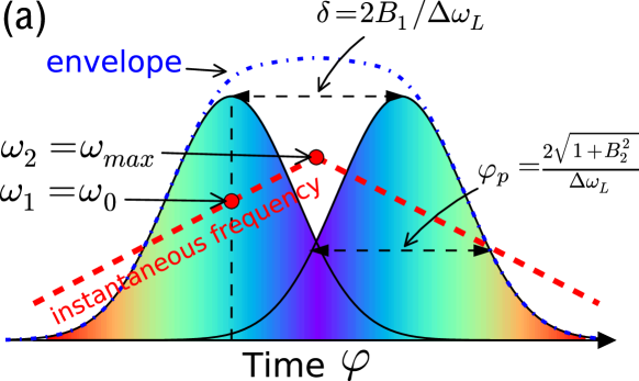
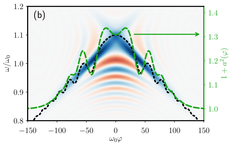
Figure 1: Schematic sketch of the two-pulse model for generating optimized laser pulses for narrowband nonlinear ICS (a). Wigner function of the recombined two-pulse for $\boldsymbol{B}=\{1.4,4.5,-4.6\}$ (b). The black curve is the analytical expression for the instantaneous frequency $\omega_{L}(\varphi)$, the green dashed curve is the analytical instantaneous $1+a^{2}(\varphi)$.

The temporal structure of the recombined pulse can be found analytically by the inverse Fourier transform of Eq. (5), yielding the complex amplitude $a_{\perp}(\varphi)=a(\varphi)e^{-i\Phi(\varphi)}$, where $a(\varphi)$ is the time-dependent envelope, and $\Phi(\varphi)$ is the temporal phase of the two-pulse. The instantaneous frequency in the recombined pulse is given by $\omega_{L}(\varphi)=\mathrm{d}\Phi(\varphi)/\mathrm{d}\varphi$, which is a slowly varying function Maroli et al. (2018). Explicit analytical expressions are lengthy, and given in the Supplementary Material. In the limit $\boldsymbol{B}=\boldsymbol{0}$, we re-obtain the Fourier-limited Gaussian pulse with the amplitude $a_{0}$ and temporal r.m.s. duration $\Delta\varphi=1/\Delta\omega_{L}$, Eq. (4). For nonzero values of $\boldsymbol{B}$ the resulting laser pulse will be stretched, with a non-Gaussian envelope in general, and with a lower effective peak amplitude than the Fourier limited pulse. It can be thought of as a superposition of two interfering linearly chirped Gaussian pulses with a delay of $\delta=2B_{1}/\Delta\omega_{L}$, each with a full-width at $1/e$ duration $\varphi_{p}=2\sqrt{1+B_{2}^{2}}/\Delta\omega_{L}$, see Fig. 1 (a). The Wigner function characterizing such a recombined two-pulse is shown in Fig. 1(b), together with the instantaneous frequency $\omega_{L}(\varphi)$ (dashed black curve) and instantaneous $1+a^{2}(\varphi)$ (dashed green curve).

The goal is to optimize $\boldsymbol{B}$ such that the compensation condition (2) is fulfilled as good as possible, see green and black curves in Fig. 1(b). The optimal values of $\boldsymbol{B}$ depend on $a_{0}$ and the available laser bandwidth. We mention here that the stretching of the pulse alone leads to some improvement of the spectral brightness already since the effective $a_{0}$ is lowered. However, as we shall see later when comparing with an unchirped matched Gaussian pulse, the optimal pulse chirping improves the spectral brightness much further.

The on-axis ICS gamma photon spectral density of an optimized laser pulse scattered from a counterpropagating electron with $\gamma\gg 1$, assuming quantum recoil and radiation reaction can be still neglected , can then be written as Sup

$$\left.\frac{\mathrm{d}^{2}N}{\mathrm{d}y\mathrm{d}\Omega}\right|_{\theta=\pi}=\mathcal{N}\left|\intop_{-\infty}^{+\infty}\!\mathrm{d}\varphi\>a_{\perp}(\varphi)\,e^{i\omega_{0}y\left(\varphi+\int_{-\infty}^{\varphi}a(\varphi^{\prime})^{2}\mathrm{d}\varphi^{\prime}\right)}\right|^{2}\,,$$ (6)

with $y=\omega^{\prime}/(4\gamma^{2}\omega_{0})$ as the normalized frequency, $\theta$ is the polar angle, and normalization $\mathcal{N}=e^{2}y\gamma^{2}\omega_{0}^{2}/\pi^{2}$. The on-axis scattered photon spectrum depends on the values of $\boldsymbol{B}$, as illustrated in Fig. 2(a), where the case of $a_{0}=2$ and $\Delta\omega_{L}/\omega_{0}=0.1$ is presented. The black dashed curve shows the spectrum for the unchirped laser pulse with $\boldsymbol{B}=\boldsymbol{0}$, while the blue solid line shows the spectrum for the optimized values $\boldsymbol{B}=\{1.4,4.5,-4.6\}$ with rms bandwidth $\Delta y=0.0178$. The corresponding normalized laser pulse vector potential shapes are shown in Fig. 2(b) with the same color code.

For the chirped pulse (blue solid line), both the envelope and the waveform are presented, and one can measure that the frequency in the wings of the laser pulse is lower than in the center, where the intensity is higher. For comparison, we also employ the notion of the matched Gaussian pulse—a pulse that has the same amplitude as the chirped pulse ($a_{\mathrm{eff}}=0.58$), and the same energy content, but the frequency is constant and is equal to $\omega_{0}$ Sup . The envelope of the matched Gaussian pulse and the corresponding ICS photon spectrum are shown by red curves in Fig. 2(b) and (a), respectively. One can see that, by choosing the optimal chirp parameters, the peak of the scattered photon spectrum is in this case 4 times higher and the bandwidth is significantly narrower than the case of the matched unchirped Gaussian pulse.

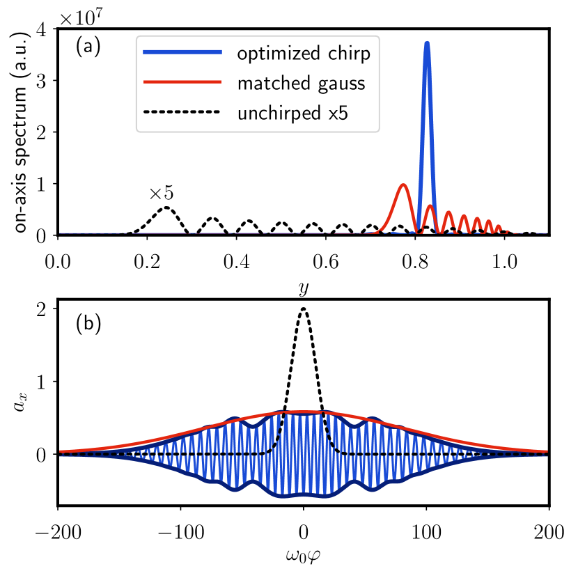
Figure 2: (a) On-axis scattered photon spectra for $a_{0}=2$, $\Delta\omega_{L}/\omega_{0}=0.1$ for different values of parameters $\boldsymbol{B}$. The spectrum for the unchirped case with $\boldsymbol{B}=\boldsymbol{0}$ is drawn with dashed black line. Note, that for visibility, the spectrum has been multiplied by 5. The case of the optimal set of parameters $\boldsymbol{B}=\{1.4,4.5,-4.6\}$ is shown with a blue curve. The red cure demonstrates the on-axis scattered photon spectrum for the matched unchirped Gaussian pulse (described in the text). (b) Corresponding amplitudes $a(\varphi)$ of the normalized laser vector potential.

We now develop a model to predict the optimal chirp parameters $\boldsymbol{B}$ for generation of a narrowband ICS spectrum. As discussed above, the recombined optimized laser pulse can be seen as the coherent superposition of two delayed oppositely linearly chirped Gaussian pulses. If the delay is too large this will result in two separate pulses and the optimization condition (2) cannot be fulfilled.

First, for optimal pulse overlap the delay between the two pulses $\delta$ should roughly equal the duration of each of the pulses $\varphi_{p}$, hence, $B_{1}=\chi\sqrt{1+B_{2}^{2}}$, with $\chi=\mathcal{O}(1)$ as a factor of proportionality . Second, the interference of two pulses should be mostly constructive and the two-pulse should contain the maximum possible amount of photons, which determines $B_{0}(B_{1},B_{2})$, see Eq. (8) below, by requiring that the argument of the cosine in the analytical expression for $a^{2}(\varphi)$ Sup is $2\pi n$ with integer $n$.

Finally, but most importantly, we match the linear chirp given by parameter $B_{2}$ to the change of the envelope. For doing this, one only needs two values of instantaneous frequency $\omega_{L}(\phi)$ Sup : one at the center of each Gaussian pulses, $\omega_{1}=\omega_{0}$, and the other in the middle of the two-pulse, $\omega_{2}\simeq\omega_{0}-{\chi B_{2}\Delta\omega_{L}}/{\sqrt{1+B_{2}^{2}}}$. This is outlined in Fig. 1 (a), where instantaneous frequency is schematically drawn with the dashed red line, and two points used for slope matching are shown with red dots. The compensation condition for narrowband emission now turns into

$$\frac{\omega_{1}}{1+a^{2}(-\delta/2)}=\frac{\omega_{2}}{1+a^{2}(0)}\,,$$ (7)

which provides an equation for $B_{2}$. In the limit $|B_{2}|\gg 1$, after straightforward algebraic calculations, we find expressions for all three parameters as functions of laser bandwidth and $a_{0}$,

$$\begin{split}B_{2}&=-\frac{a_{0}^{2}}{4\chi}\frac{\omega_{0}}{\Delta\omega_{L}}\left(4e^{-\chi^{2}}-1-\chi\frac{\Delta\omega_{L}}{\omega_{0}}\right)\,,\\ B_{1}&=\chi\sqrt{1+B_{2}^{2}}\,,\\ B_{0}&=\frac{\chi^{2}B_{2}}{2}-\frac{1}{4}\arctan B_{2}+n\pi\,,\end{split}$$ (8)

that produce laser pulses which compensate the nonlinear spectrum broadening and significantly reduce the bandwidth of backscattered X-rays.

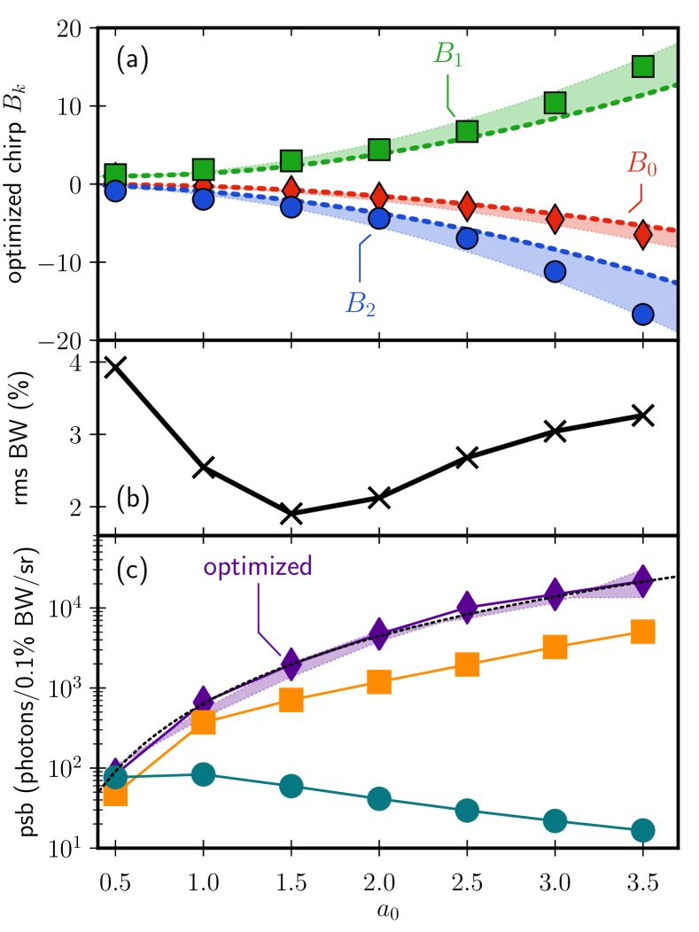
Figure 3: (a) Optimal chirp parameters $B_{0}$ (red diamonds), $B_{1}$ (green squares) and $B_{2}$ (blue circles) that lead to the narrowest on-axis scattered photon spectrum and obtained from simulations, as functions of $a_{0}$ for $\Delta\omega_{L}/\omega_{0}=0.1$. Shaded areas of corresponding colors are the model predictions, Eqns. (8). (b) Relative rms bandwidth of the on-axis photon spectrum for the optimally chirped pulse. (c) Peak spectral brightness (psb) of the on-axis scattered photons as a function of $a_{0}$ for the optimally chirped pulse (purple diamonds) and compared to matched Gaussian (orange squares) and unoptimized cases (cyan circles). The black dotted curve represents a fit $f(a_{0})=637\,a_{0}^{2.8}$ of the optimized case, the shaded are corresponds to peak spectral brightness predicted using model parameters just like in (a).

Numerical optimization was carried out in order to find optimal sets of parameters $\boldsymbol{B}$ that yields the narrowest rms ICS spectrum for various $a_{0}$ and laser bandwidth $\Delta\omega_{L}/\omega_{0}=0.1$. The results are shown in Fig. 3, and compared to the analytical model predictions, Eqns. (8). The symbols in Fig. 3 (a) refer to the numerically optimized parameters $\boldsymbol{B}$, while the shaded areas correspond to the model predictions with varying $\chi=0.95\ldots 1$ with the dotted curves at $\chi=1$. Note there are some discrepancies between the numerical optimization and the analytical model for small $a_{0}$ because we assumed $B_{2}\gg 1$ in order to solve the equations to arrive at (8).

Fig. 3 (b) shows a relative rms bandwidth of the ICS photons, which is well below 4% throughout. It is evident there is an optimal range of $a_{0}$ for the given laser bandwidth around $a_{0}=1.5$ where the bandwidth of the ICS photons is smallest. This optimal region shifts to higher $a_{0}$ for larger laser bandwidth.

For large values of $a_{0}>3.5$, the quality of the photon spectrum somewhat decreases. We attribute this to the fact, that for high values of $a_{0}$, the amount of chirp stretches the pulses very long and the delay between pulses leads to the beating of two Gaussians such that the envelope of the two-pulse is not smooth anymore. According to our model, for the optimally chirped pulses the effective $a_{\mathrm{eff}}\approx 1.76\times\sqrt{\Delta\omega_{L}/\omega_{0}}$ for $|B_{2}|\gg 1$, independent of the initial $a_{0}$. We have performed studies for different values of $\Delta\omega_{L}/\omega_{0}$ and found similar optimization but extending to larger $a_{0}$ for larger bandwidth.

Fig. 3(c) shows the on-axis peak spectral brightness of the ICS photons as a function of $a_{0}$ for the numerically optimized chirped pulses (purple diamonds). The purple shaded area corresponds to the optimized model parameters Eqns. (8) with the same variation as in Fig. 3 (a), showing a very good agreement and robustness. The case of $a_{0}=2$ is the same as shown in Fig. 2. Our simulations indicate that the peak spectral brightness for optimally chirped pulses grows $\propto a_{0}^{2.8}$ (black dotted curve). For comparison, we also show the completely unchirped pulses (green circles) and matched gaussians (orange squares). The peak spectral brightness for optimally chirped pulse exceeds the matched Gaussian pulse by a factor of $4\ldots 5$.

We have presented a simple two-pulse scheme for the compensation of non-linear broadening effects in inverse Compton scattering gamma ray sources based on the spectral synthesis of optimized chirped laser pulses. We developed a model to predict the required spectral phase in dependence on the laser intensity and bandwidth. To verify the robustness of our scheme with regard to 3D effects we numerically simulated electron trajectories and the radiation emission using Liénard-Wiechert potentials in the far field Jackson (1998) for a realistic scenario (Figure 4): A $270\text{\,}\mathrm{MeV}$ LPA electron beam with $2.2\text{\,}\%$ energy spread and $0.2\text{\,}\mathrm{m}\mathrm{m}\,\mathrm{m}\rad$ normalized emittance, beam size $1.8\text{\,}\mathrm{\SIUnitSymbolMicro m}$ and duration $10\text{\,}\mathrm{fs}$ Lundh et al. (2011); Plateau et al. (2012); Weingartner et al. (2012), is colliding with a Gaussian laser pulse of waist $w_{0}=$20\text{\,}\mathrm{\SIUnitSymbolMicro m}$$ within the paraxial approximation Harvey et al. (2016); Maroli et al. (2018), $a_{0}=2$, $\omega_{0}=$1.55\text{\,}\mathrm{eV}$$, and the temporal chirping taken from the numerical optimization in Fig. 3.

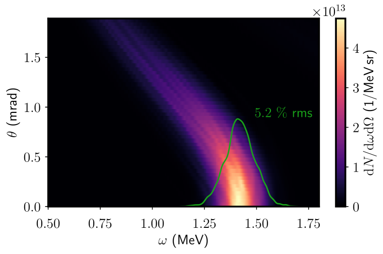
Figure 4: Simulated spectral-angular Compton photon distribution for a $50\text{\,}\mathrm{pC}$ realistic electron beam interacting with a focused laser pulse. The green curve is an on-axis lineout.

Our model predictions can serve as initial conditions for active feedback optimization of inverse Compton sources, e.g. using machine learning techniques. The optimal control of the temporal laser pulse structure has been successfully demonstrated already, e.g. for the optimization of laser accelerated electron beams and x-ray production Streeter et al. (2018); Dann et al. . The optimal chirping of the scattering pulse could be included into an overall feedback loop. Depending on the desired bandwidth of the ICS the other contributions to the total bandwidth, such as the electron energy spread and emittance, could be optimized alongside the temporal spectral shape of the scattering laser pulse by choosing proper goal functions for optimization.

D. S. acknowledges fruitful discussions with A. G. R. Thomas and S. Dann. This work was funded in part by the US ARO grant no. W911NF-16-1-0044 and by the Helmholtz Association (Young Investigators Group VH-NG-1037).

Part I Supplementary Material

I Analytic Results for the Two-Pulse

Here we provide explicit formulas for the vector potential of the recombined two-pulse $a_{\perp}(\varphi)$, its envelope $a(\varphi)$, and local frequency $\omega_{L}(\varphi)$. First, by calculating the inverse Fourier transformation of the modulated spectrum, Eq. (5) of the main text, we immediately find the complex scalar amplitude

$$a_{\perp} =\frac{a_{0}}{2\sqrt[4]{1+B_{2}^{2}}}e^{-i\omega_{0}\varphi}\left(e^{-\frac{c_{-}}{2}(1+iB_{2})+iB_{0}+\frac{i}{2}\arctan B_{2}}+e^{-\frac{c_{+}}{2}(1-iB_{2})-iB_{0}-\frac{i}{2}\arctan B_{2}}\right)$$ (S.1)

with

$$c_{\pm} =\frac{(B_{1}\pm\varphi\Delta\omega_{L})^{2}}{1+B_{2}^{2}}\,,$$ (S.2)

and $\varphi=t-z$. The real vector potential of a circularly polarized laser pulse is related to $a_{\perp}$ by $\boldsymbol{a}_{\perp}=\Re[a_{\perp}\boldsymbol{\epsilon}]$ with $\boldsymbol{\epsilon}=\boldsymbol{e}_{x}+i\boldsymbol{e}_{y}$.

The squared envelope of the laser pulse is given by

$$a^{2}(\varphi) =\boldsymbol{a}_{\perp}^{2}=|a_{\perp}|^{2}=\frac{a_{0}^{2}}{2\sqrt{1+B_{2}^{2}}}e^{-\xi}\left[\cosh 2d_{0}\varphi+\cos\zeta\right]$$ (S.3)

where we introduced the following abbreviations

$$d_{0} =\frac{B_{1}\Delta\omega}{1+B_{2}^{2}}\,,\qquad\xi=\frac{B_{1}^{2}+\varphi^{2}\Delta\omega^{2}_{L}}{1+B_{2}^{2}}\,,\qquad\zeta=2B_{0}-B_{2}\xi+\arctan B_{2}\,.$$ (S.4)

An important quantity is the infinite integral over the squared vector potential envelope,

$$\intop_{-\infty}^{\infty}\!\mathrm{d}\varphi\>a^{2}(\varphi)=\frac{a_{0}^{2}\sqrt{\pi}}{2}\frac{1}{\Delta\omega_{L}}\left[1+\frac{e^{-\frac{B_{1}^{2}}{1+B_{2}^{2}}}}{(1+B_{2}^{2})^{\frac{1}{4}}}\,\cos\left({2B_{0}-\frac{B_{1}^{2}B_{2}}{1+B_{2}^{2}}+\frac{1}{2}\arctan B_{2}}\right)\right]\,.$$ (S.5)

When the cosine term is maximised, i.e. its argument a multiple of $2\pi$, then the interference between the two sub-pulses is mostly constructive.

Because $a_{\perp}=a\,e^{-i\Phi(\varphi)}$ we can write $\Phi=i\log\frac{a_{\perp}}{a}$, and

$$\omega_{L}(\varphi) =\frac{\mathrm{d}\Phi}{\mathrm{d}\varphi}=-\frac{{\rm Im}\,[a_{\perp}^{\prime}a_{\perp}^{*}]}{a^{2}}=\omega_{0}-d_{0}B_{2}+d_{0}\>\frac{\varphi\frac{\Delta\omega B_{2}}{B_{1}}\sinh 2d_{0}\varphi-\sin\zeta}{\cosh 2d_{0}\varphi+\cos\zeta}\,.$$ (S.6)

II Defining the Matched Gaussian Pulse

We match the a Gaussian with constant frequency $\omega_{0}$ to the two-pulse, having the same effective peak amplitude and total energy in the pulse,

$$a_{\mathrm{matched}}(\varphi)=a_{\mathrm{eff}}\,e^{-i\omega_{0}\varphi}\,e^{-\varphi^{2}/2\Delta\varphi_{\mathrm{eff}}^{2}}\,.$$ (S.7)

First, the amplitude is matched by evaluating Eq. (S.3) at $\varphi=0$ with the approximation $\zeta\to 0$, yielding

$$a_{\mathrm{eff}}^{2} =a_{0}^{2}\>\frac{e^{-\frac{B_{1}^{2}}{1+B_{2}^{2}}}}{\sqrt{1+B^{2}_{2}}}\,.$$ (S.8)

Second, the pulse duration is matched by the requirement that both the chirped two-pulse and the matched Gaussian have the same energy,

$$w=\int\mathrm{d}\varphi\left|\frac{\mathrm{d}a_{\perp}}{\mathrm{d}\varphi}\right|^{2}\,,$$ (S.9)

i.e.

$$\Delta\varphi_{\mathrm{eff}}=\frac{w}{\sqrt{\pi}\omega_{0}^{2}a_{\mathrm{eff}}^{2}}\,.$$ (S.10)

III Derivation of the Formula for the on-axis Spectrum

Under the assumption that we can use classical electrodynamics to calculate the radiation spectrum, the energy and angular differential photon distribution is given by Jackson (1998)

$$\frac{\mathrm{d}N}{\mathrm{d}\omega^{\prime}\mathrm{d}\Omega}=\frac{\omega^{\prime}}{4\pi^{2}}|\boldsymbol{n}^{\prime}\times(\boldsymbol{n}^{\prime}\times\boldsymbol{j})|^{2}\,,$$ (S.11)

with the Fourier transformed electron current

$$\boldsymbol{j}(\omega^{\prime},\boldsymbol{n}^{\prime})=-e\int\!\mathrm{d}s\,\boldsymbol{u}(s)\,e^{i\omega^{\prime}[t(s)-\boldsymbol{n}^{\prime}\cdot\boldsymbol{x}(s)]}\,,$$ (S.12)

and $\boldsymbol{n}^{\prime}$ the direction under which the radiation is observed. Here, $s$ denotes the electron’s proper time, parametrizing the electron orbits $t(s),\boldsymbol{x}(s)$ and four-velocity components $\gamma(s)=\mathrm{d}t/\mathrm{d}s=\sqrt{1+\boldsymbol{u}^{2}}$ and $\boldsymbol{u}=\mathrm{d}\boldsymbol{x}/\mathrm{d}s$, which is a solution of the Lorentz force equation

$$\frac{\mathrm{d}\boldsymbol{u}}{\mathrm{d}s}=\frac{e}{m}(\gamma\boldsymbol{E}+\boldsymbol{u}\times\boldsymbol{B})\,.$$ (S.13)

For on-axis radiation, $\boldsymbol{n}^{\prime}=-\boldsymbol{e}_{z}$, the double vector product can be simplified to

$$|\boldsymbol{n}^{\prime}\times(\boldsymbol{n}^{\prime}\times\boldsymbol{j})|^{2}=|\boldsymbol{j}_{\perp}|^{2}\,,$$ (S.14)

and with $\boldsymbol{u}_{\perp}=-\boldsymbol{a}_{\perp}$ and changing integration variables from proper time to laser phase $\varphi=t-z$ via $\mathrm{d}\varphi/\mathrm{d}s\approx 2\gamma$ (for initial value of $\gamma\gg 1$), (S.11) turns into

$$\left.\frac{\mathrm{d}N}{\mathrm{d}\omega^{\prime}\mathrm{d}\Omega}\right|_{\mathrm{on-axis}}=\frac{e^{2}\omega^{\prime}}{4\pi^{2}(2\gamma)^{2}}\>\left|\int\!\mathrm{d}\varphi\,\boldsymbol{a}_{\perp}\>e^{i\omega^{\prime}[t(\varphi)+z(\varphi)]}\right|^{2}\,.$$ (S.15)

By noting that $t(\varphi)+z(\varphi)=(2\gamma)^{-1}\int\!\mathrm{d}\varphi[\gamma(\varphi)+u_{z}(\varphi)]$, with $\gamma(\varphi)+u_{z}(\varphi)=(1+\boldsymbol{a}_{\perp}^{2})/(2\gamma)$, the definition of the normalized frequency of the emitted photon, $y=\omega^{\prime}/(4\gamma^{2}\omega_{0})$ we eventually arrive at Eq. (6) of the main text. In Fig. 5 we show the on-axis spectra for optimized laser pulses of various intensities and bandwidth $\Delta\omega_{L}/\omega_{0}=0.1$.

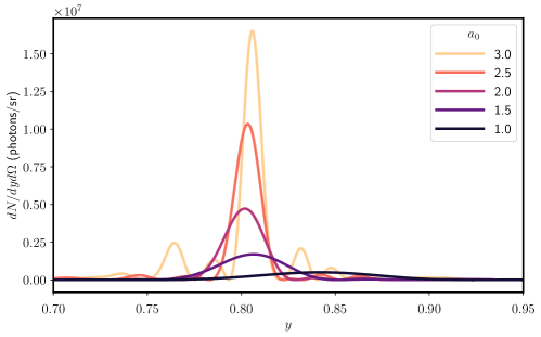
Figure 5: On-axis photon spectra from optimized laser pulses with the chirping parameters $\boldsymbol{B}$ calculated using the model Eqns. (8) with $\chi=1$.

References

- Scott Carman et al. (1996) T. Scott Carman, V. Litveninko, J. Madey, C. Neuman, B. Norum, P. G. O’Shea, N. Russell Roberson, C. Y. Scarlett, E. Schreiber, and H. R. Weller, “The TUNL-FELL inverse Compton -ray source as a nuclear physics facility,” Nucl. Instruments Methods Phys. Res. Sect. A Accel. Spectrometers, Detect. Assoc. Equip. 378, 1–20 (1996).
- Bertozzi et al. (2008) W. Bertozzi, J. A. Caggiano, W. K. Hensley, M. S. Johnson, S. E. Korbly, R. J. Ledoux, D. P. McNabb, E. B. Norman, W. H. Park, and G. A. Warren, “Nuclear resonance fluorescence excitations near 2 MeV in 235U and 239Pu,” Phys. Rev. C - Nucl. Phys. 78, 041601 (2008).
- Albert et al. (2010) F. Albert, S. G. Anderson, D. J. Gibson, C. A. Hagmann, M. S. Johnson, M. Messerly, V. Semenov, M. Y. Shverdin, B. Rusnak, A. M. Tremaine, F. V. Hartemann, C. W. Siders, D. P. McNabb, and C. P. J. Barty, “Characterization and applications of a tunable, laser-based, MeV-class Compton-scattering -ray source,” Phys. Rev. ST Accel. Beams 13, 070704 (2010).
- Albert et al. (2011) F. Albert, S. G. Anderson, D. J. Gibson, R. A. Marsh, S. S. Wu, C. W. Siders, C. P. J. Barty, and F. V. Hartemann, “Design of narrow-band Compton scattering sources for nuclear resonance fluorescence,” Phys. Rev. ST Accel. Beams 14, 050703 (2011).
- Quiter et al. (2011) B. J. Quiter, B. A. Ludewigt, V. V. Mozin, C. Wilson, and S. Korbly, “Transmission nuclear resonance fluorescence measurements of 238U in thick targets,” Nucl. Instruments Methods Phys. Res. Sect. B Beam Interact. with Mater. Atoms 269, 1130–1139 (2011).
- Rykovanov et al. (2014) S. G. Rykovanov, C. G. R. Geddes, J.-L. Vay, C. B. Schroeder, E. Esarey, and W. P. Leemans, “Quasi-monoenergetic femtosecond photon sources from Thomson Scattering using laser plasma accelerators and plasma channels,” J. Phys. B 47, 234013 (2014).
- Albert and Thomas (2016) F. Albert and A. G. R. Thomas, “Applications of laser wakefield accelerator-based light sources,” Plasma Phys. Control. Fusion 58, 103001 (2016).
- Gales et al. (2018) S. Gales, K. A. Tanaka, D. L. Balabanski, F. Negoita, D. Stutman, O. Tesileanu, C. A. Ur, D. Ursescu, I. Andrei, S. Ataman, M. O. Cernaianu, L. D’Alessi, I. Dancus, B. Diaconescu, N. Djourelov, D. Filipescu, P. Ghenuche, D. G. Ghita, C. Matei, K. Seto, M. Zeng, and N. V. Zamfir, “The extreme light infrastructure–nuclear physics (ELI-NP) facility: new horizons in physics with 10 PW ultra-intense lasers and 20 MeV brilliant gamma beams,” Reports Prog. Phys. 81, 094301 (2018).
- Krämer et al. (2018) J. M. Krämer, A. Jochmann, M. Budde, M. Bussmann, J. P. Couperus, T. E. Cowan, A. Debus, A. Köhler, M. Kuntzsch, A. Laso García, U. Lehnert, P. Michel, R. Pausch, O. Zarini, U. Schramm, and A. Irman, “Making spectral shape measurements in inverse Compton scattering a tool for advanced diagnostic applications,” Sci. Rep. 8, 1398 (2018).
- Nedorezov et al. (2004) V. G. Nedorezov, A. A. Turinge, and Y. M. Shatunov, “Photonuclear experiments with Compton-backscattered gamma beams,” Physics-Uspekhi 47, 341–358 (2004).
- Carpinelli and Serafini (2009) M. Carpinelli and L. Serafini, “Compton sources for X/ rays: Physics and applications,” Nucl. Instrum. Methods Phys. Res., Sect. A 608, S1–S120 (2009).
- Albert et al. (2014) F. Albert, A. G. R. Thomas, S. P. D. Mangles, S. Banerjee, S. Corde, A. Flacco, M. Litos, D. Neely, J. Vieira, Z. Najmudin, R. Bingham, C. Joshi, and T. Katsouleas, “Laser wakefield accelerator based light sources: potential applications and requirements,” Plasma Phys. Control. Fusion 56, 084015 (2014).
- Mangles et al. (2004) S. P. D. Mangles, C. D. Murphy, Z. Najmudin, A. G. R. Thomas, J. L. Collier, A. E. Dangor, E. J. Divall, P. S. Foster, J. G. Gallacher, C. J. Hooker, D. A. Jaroszynski, A. J. Langley, W. B. Mori, P. A. Norreys, F. S. Tsung, R. Viskup, B. R. Walton, and K. Krushelnick, “Monoenergetic beams of relativistic electrons from intense laser-plasma interactions,” Nature 431, 535–538 (2004).
- Leemans et al. (2006) W. P. Leemans, B. Nagler, A. J. Gonsalves, Cs. Tóth, K. Nakamura, C. G. R. Geddes, E. Esarey, C. B. Schroeder, and S. M. Hooker, “GeV electron beams from a centimetre-scale accelerator.” Nat. Phys. 2, 696 (2006).
- Esarey et al. (2009) E. Esarey, C. B. Schroeder, and W. P. Leemans, “Physics of laser-driven plasma-based electron accelerators,” Rev. Mod. Phys. 81, 1229–1285 (2009).
- Curatolo et al. (2017) C. Curatolo, I. Drebot, V. Petrillo, and L. Serafini, “Analytical description of photon beam phase spaces in inverse Compton scattering sources,” Phys. Rev. Accel. Beams 20, 080701 (2017).
- Ranjan et al. (2018) N. Ranjan, B. Terzić, G. A. Krafft, V. Petrillo, I. Drebot, and L. Serafini, “Simulation of inverse Compton scattering and its implications on the scattered linewidth,” Phys. Rev. Accel. Beams 21, 030701 (2018).
- Hartemann et al. (1996) F. V. Hartemann, A. L. Troha, N. C. Luhmann Jr., and Z. Toffano, “Spectral analysis of the nonlinear relativistic Doppler shift in ultrahigh intensity Compton scattering,” Phys. Rev. E 54, 2956 (1996).
- Krafft (2004) G. A. Krafft, “Spectral Distributions of Thomson-Scattered Photons from High-Intensity Pulsed Lasers,” Phys. Rev. Lett. 92, 204802 (2004).
- Hartemann et al. (2010) F. V. Hartemann, F. Albert, C. W. Siders, and C. P. J. Barty, “Low-Intensity Nonlinear Spectral Effects in Compton Scattering,” Phys. Rev. Lett. 105, 130801 (2010).
- Maroli et al. (2013) C. Maroli, V. Petrillo, P. Tomassini, and L. Serafini, “Nonlinear effects in Thomson backscattering,” Phys. Rev. Spec. Top. - Accel. Beams 16, 030706 (2013).
- Kharin et al. (2016) V. Yu. Kharin, D. Seipt, and S. G. Rykovanov, “Temporal laser-pulse-shape effects in nonlinear Thomson scattering,” Phys. Rev. A 93, 063801 (2016).
- Chen et al. (2013) S. Chen, N. D. Powers, I. Ghebregziabher, C. M. Maharjan, C. Liu, G. Golovin, S. Banerjee, J. Zhang, N. Cunningham, A. Moorti, S. Clarke, S. Pozzi, and D. P. Umstadter, “MeV-Energy X Rays from Inverse Compton Scattering with Laser-Wakefield Accelerated Electrons,” Phys. Rev. Lett. 110, 155003 (2013).
- Sarri et al. (2014) G. Sarri, D. J. Corvan, W. Schumaker, J. M. Cole, A. Di Piazza, H. Ahmed, C. Harvey, C. H. Keitel, K. Krushelnick, S. P. D. Mangles, Z. Najmudin, D. Symes, A. G. R. Thomas, M. Yeung, Z. Zhao, and M. Zepf, “Ultrahigh Brilliance Multi-MeV -Ray Beams from Nonlinear Relativistic Thomson Scattering,” Phys. Rev. Lett. 113, 224801 (2014).
- Khrennikov et al. (2015) K. Khrennikov, J. Wenz, A. Buck, J. Xu, M. Heigoldt, L. Veisz, and S. Karsch, “Tunable All-Optical Quasimonochromatic Thomson X-Ray Source in the Nonlinear Regime,” Phys. Rev. Lett. 114, 195003 (2015).
- Cole et al. (2018) J. M. Cole, K. T. Behm, E. Gerstmayr, T. G. Blackburn, J. C. Wood, C. D. Baird, M. J. Duff, C. Harvey, A. Ilderton, A. S. Joglekar, K. Krushelnick, S. Kuschel, M. Marklund, P. McKenna, C. D. Murphy, K. Poder, C. P. Ridgers, G. M. Samarin, G. Sarri, D. R. Symes, A. G. R. Thomas, J. Warwick, M. Zepf, Z. Najmudin, and S. P. D. Mangles, “Experimental Evidence of Radiation Reaction in the Collision of a High-Intensity Laser Pulse with a Laser-Wakefield Accelerated Electron Beam,” Phys. Rev. X 8, 011020 (2018).
- Ghebregziabher et al. (2013) I. Ghebregziabher, B. A. Shadwick, and D. Umstadter, “Spectral Bandwidth Reduction of Thomson Scattered Light by Pulse Chirping,” Phys. Rev. ST Accel. Beams 16, 030705 (2013).
- Terzić et al. (2014) B. Terzić, K. Deitrick, A. S. Hofler, and G. A. Krafft, “Narrow-Band Emission in Thomson Sources Operating in the High-Field Regime,” Phys. Rev. Lett. 112, 074801 (2014).
- Seipt et al. (2015) D. Seipt, S. G. Rykovanov, A. Surzhykov, and S. Fritzsche, “Narrowband inverse Compton scattering x-ray sources at high laser intensities,” Phys. Rev. A 91, 033402 (2015).
- Rykovanov et al. (2016) S. G. Rykovanov, C. G. R. Geddes, C. B. Schroeder, E. Esarey, and W. P. Leemans, “Controlling the spectral shape of nonlinear Thomson scattering with proper laser chirping,” Phys. Rev. Accel. Beams 19, 030701 (2016).
- Kharin et al. (2018) V. Yu. Kharin, D. Seipt, and S. G. Rykovanov, “Higher-Dimensional Caustics in Nonlinear Compton Scattering,” Phys. Rev. Lett. 120, 044802 (2018).
- Maroli et al. (2018) C. Maroli, V. Petrillo, I. Drebot, L. Serafini, B. Terzić, and G. A. Krafft, “Compensation of non-linear bandwidth broadening by laser chirping in Thomson sources,” J. Appl. Phys. 124, 063105 (2018).
- Note (1) Quantum recoil and spin effects can be neglected for electron energies below 200 MeV, but could easily be included and do not change any qualitative findings on the optimal chirp Seipt et al. (2015). Radiation reaction effects and recoil broadening effects due to multi-photon emission can be neglected when the number of scatterings per electron is less than one, , i.e. for Rykovanov et al. (2014); Terzić et al. (2014). Otherwise the recoil contribution to the bandwidth is proportional to .
- (34) For details see Supplementary Material.
- Note (2) Due to symmetry reasons, produces the same laser pulse as . Moreover, and need to have opposite sign, we chose here .
- Jackson (1998) J. D. Jackson, Classical Electrodynamics, 3rd ed. (Wiley, 1998).
- Lundh et al. (2011) O. Lundh, J. Lim, C. Rechatin, L. Ammoura, A. Ben-Ismaïl, X. Davoine, G. Gallot, J-P. Goddet, E. Lefebvre, V. Malka, and J. Faure, “Few femtosecond, few kiloampere electron bunch produced by a laser–plasma accelerator,” Nat. Phys. 7, 219–222 (2011).
- Plateau et al. (2012) G. R. Plateau, C. G. R. Geddes, D. B. Thorn, M. Chen, C. Benedetti, E. Esarey, A. J. Gonsalves, N. H. Matlis, K. Nakamura, C. B. Schroeder, S. Shiraishi, T. Sokollik, J. van Tilborg, Cs. Toth, S. Trotsenko, T. S. Kim, M. Battaglia, Th. Stöhlker, and W. P. Leemans, “Low-Emittance Electron Bunches from a Laser-Plasma Accelerator Measured using Single-Shot X-Ray Spectroscopy,” Phys. Rev. Lett. 109, 064802 (2012).
- Weingartner et al. (2012) R. Weingartner, S. Raith, A. Popp, S. Chou, J. Wenz, K. Khrennikov, M. Heigoldt, A. R. Maier, N. Kajumba, M. Fuchs, B. Zeitler, F. Krausz, S. Karsch, and F. Grüner, “Ultralow emittance electron beams from a laser-wakefield accelerator,” Phys. Rev. Spec. Top. - Accel. Beams 15, 111302 (2012).
- Harvey et al. (2016) C. Harvey, M. Marklund, and A. R. Holkundkar, “Focusing effects in laser-electron Thomson scattering,” Phys. Rev. Accel. Beams 19, 094701 (2016).
- Streeter et al. (2018) M. J. V. Streeter, S. J. D. Dann, J. D. E. Scott, C. D. Baird, C. D. Murphy, S. Eardley, R. A. Smith, S. Rozario, J.-N. Gruse, S. P. D. Mangles, Z. Najmudin, S. Tata, M. Krishnamurthy, S. V. Rahul, D. Hazra, P. Pourmoussavi, J. Osterhoff, J. Hah, N. Bourgeois, C. Thornton, C. D. Gregory, C. J. Hooker, O. Chekhlov, S. J. Hawkes, B. Parry, V. A. Marshall, Y. Tang, E. Springate, P. P. Rajeev, A. G. R. Thomas, and D. R. Symes, “Temporal feedback control of high-intensity laser pulses to optimize ultrafast heating of atomic clusters,” Appl. Phys. Lett. 112, 244101 (2018).
- (42) S. Dann et al., To appear.