Introspection Learning

Abstract

Traditional reinforcement learning agents learn from experience, past or present, gained through interaction with their environment. Our approach synthesizes experience, without requiring an agent to interact with their environment, by asking the policy directly “Are there situations $X$, $Y$, and $Z$, such that in these situations you would select actions $A$, $B$, and $C$?” In this paper we present Introspection Learning, an algorithm that allows for the asking of these types of questions of neural network policies. Introspection Learning is reinforcement learning algorithm agnostic and the states returned may be used as an indicator of the health of the policy or to shape the policy in a myriad of ways. We demonstrate the usefulness of this algorithm both in the context of speeding up training and improving robustness with respect to safety constraints.

1 Introduction

One notable feature of human learners is that we are able to carry out counter-factual reasoning over unrealized events. That is, we contemplate potential answers to questions of the form, “What would I do in situations $X$, $Y$, and $Z$?” A related, and perhaps more pertinent, form of question is, “Are there situations $X$, $Y$, and $Z$, such that in these situations I would select actions $A$, $B$, and $C$?” In this case, the actions $A$, $B$, etc., might be actions that are likely to result in particularly good or bad outcomes, and answers $X$, $Y$, etc., can be useful, especially when they are of an unexpected nature, since they reveal potential failures of robustness (in the case of bad examples) or potential strengths (in the case of good examples). In this paper, we describe a novel approach to answering and utilizing the answers to questions of this form when asked not of a human agent, but of a reinforcement learning agent. Our approach is not based solely on the deployment of techniques from the typical machine learning toolbox, as we make crucial use of SMT-solving, which is more familiar to researchers in the field of formal methods. In the theoretical development, we capture our use of SMT-solving technology via the abstraction of what we are calling introspection oracles: oracles that may give us direct access to sets of (state, action) pairs satisfying fixed constraints with respect to the policy network.

By querying the oracle during training it is possible to generate (state, action)-pairs capturing failures/strengths of the agent with respect to properties of interest. For instance, if there are certain “obviously wrong” actions that the agent should never take (e.g., selecting a steering angle that would cause the automobile controlled by the policy network to drive off of the road when there are no obstacles or other dangers present), we query the oracle as to whether there exists states in which the agent would select such actions. Our algorithm then uses this data to train so as to improve the safety of the agent and without requiring that such potentially dangerous or costly situations be encountered in real life. It is true that such (state, action) pairs are potentially discoverable in simulation/testing, but when the set of such pairs is known beforehand we save time and improve policy robustness by generating them analytically.

In this paper, we introduce a new algorithm for reinforcement learning, which we call the Introspection Learning Algorithm, that exploits introspection oracles to improve the training and robustness of reinforcement learning (RL) agents versus baseline training algorithms. This algorithm involves modifying the underlying MDP structure and we derive theoretical results that justify these modifications. Finally, we discuss several experimental results that clearly showcase the benefits to both performance and robustness of this approach. In particular, in the case of robustness, we evaluated our results by querying the weights after training to determine numbers of Sat (examples found), Unsat (examples mathematically impossible) and Timeout (ran out of time to find or refute existence of examples) results.

The paper is organized as follows. In Section 2 we introduce the mathematical abstraction of introspection oracles and discuss briefly their embodiment as SMT-solvers. Section 3 details our Introspection Learning Algorithm. Finally, Section 4 captures our empirical results. The Appendix (Section 6) includes the proof of a basic result that justifies the modification of MDPs made in our algorithms.

Related work

Previously, Linear Programming, which is itself is a constraint solving technique, has been employed in reinforcement learning to constrain the exploration space for the agent’s policy to improve both the speed of convergence and the quality of the policy converged to (?) or as a replacement for more traditional Dynamic Programming methods in Q-Learning to solve for equilibria policies in zero-sum multi-agent Markov game MDPs (?; ?). Previous work has also been done on incorporating Quadratic Program solvers to restrict agent exploration to “safe” trajectories by constraining the output of a neural network policy (?; ?). Introspection Learning is fundamentally different from these approaches as rather than restricting the action space, or replacing our Q function, we are instead shaping our agents in policy space by asking our policy for state batches where it would satisfy stated constraints, without needing the agent to actually experience these states.

Exciting recent work on verification of neural networks (e.g., (?; ?)) is closely related the work described here. In addition to the similarity of the techniques, we are indeed capturing verification results as a robustness measure (see below). One practical distinction is that we are using the dReal solver (?), which is able to handle networks with general non-linear activations, but as a trade-off (not made in other SMT-solvers) admits the possibility of “false-positive” $\delta$-satisfiable instances. In principle, our algorithm can be used with any compatible combination of SMT-solvers and neural network architectures.

2 Introspection Oracles

In order to set the appropriate theoretical stage, we will first introduce some notation and terminology.

Definition 1.

A pre-Markov decision process (pre-MDP) consists of a set $S$ of states, a set $A$ of actions, and transition probabilities $p(s,a,s^{\prime})$ in $[0,1]$ for $s,s^{\prime}\in S$ and $a\in A$ such that $\sum_{s^{\prime}}p(s,a,s^{\prime})=1$.

Intuitively, the value $p(s,a,s^{\prime})$ is the probability $\mathbb{P}(s^{\prime}|s,a)$ transitioning from state $s$ to state $s^{\prime}$ on taking action $a$.

Definition 2.

Given a pre-Markov Decision Process (pre-MDP) $D=(S,A,p)$, a policy for $D$ assigns to each state $s$ a probability distribution $\pi(s)$ over the set $A$.

A pre-MDP is called a MDP$\backslash$R in, e.g., (?).

Often we are concerned with cases where $A$ is finite and the policies $\pi$ under consideration are deterministic in the sense that, for each state $s$, $\pi(s)(a)=0$ for all but a single element $a$ of $A$. When $p(s,a,s^{\prime})=1$ we write ${a\colon s\to s^{\prime}}$. Given a pre-MDP $D$, we denote by $\Pi(D)$ the set of all policies for $D$.

Definition 3.

A Markov decision process (MDP) consists of a pre-MDP $(S,A,p)$ together with a reward function ${r\colon S\times A\to\mathbb{R}}$ which is bounded, a subset $T\subseteq S\times A$ of terminal (state, action)-pairs, and a new state $s_{t}$ not in $S$ such that:

• For any $(s,a)\in T$, $a\colon s\to s_{t}$;

• For any $a\in A$, $a\colon s_{t}\to s_{t}$; and

• For any $a\in A$, $r(s_{t},a)=0$.

One non-standard feature of Definition 3 is that we consider terminal pairs $(s,a)\in S\times A$ rather than terminal states. This will be technically useful below. We also follow (?) in that the provision of terminal pairs modifies the pre-MDP structure in adding a dummy stable state $s_{t}$ to which all terminal states canonically transition such that subsequent transitions from $s_{t}$ have no reward. This is a technical convenience which streamlines some of the theory.

We denote by $\mathcal{M}(D)$ the set of all Markov decision processes over the pre-MDP $D$ and by $\Pi(D)$ the set of all policies over $D$. Given an MDP $M$ in $\mathcal{M}(D)$, we denote by $\textnormal{Opt}(M)$ the subset of $\Pi(D)$ consisting of those policies that are optimal for $M$. In broad strokes, inverse reinforcement learning (?) is concerned with, given a policy $\pi$ in $\Pi(D)$ (or, more often, a set of its trajectories), determining an element $M$ of $\mathcal{M}(D)$ such that $\pi$ is in $\textnormal{Opt}(M)$. We are concerned with a closely related problem.

One difference between our approach and that of inverse reinforcement learning is that instead of assuming access to a target policy $\pi$ or its trajectories, we assume that we have access to certain properties that target policies ought to have. In the simplest case, such a property is given by a subset of the set $S\times A$ of (state, action) pairs. We refer to policies with the required properties as good policies. There is considerable flexibility in the notion of goodness here, but in many cases it will be associated with safety and robustness. E.g., a good policy for driving a car would not make unexpected sharp turns when the road ahead is straight and clear of obstacles. Much of our focus is on these kinds of examples, but it is worth emphasizing that goodness could instead be associated with performance rather than safety.

In order to make the problem tractable, it is necessary to restrict to sufficiently well-behaved subsets of $S\times A$. For us, the well-behaved subsets are those definable in the first-order theory of real arithmetic with common non-linear function symbols (e.g., $\sin$, $\log$, $\max$, $\tanh$, etc.). Denote by $\mathcal{P}_{\!\!r}(X)$ the set of all such subsets of $X\subset\mathbb{R}^{n}$. With this notation in place, we arrive the definition of introspection oracle.

Definition 4.

Given policy $\pi$ in $\Pi(D)$, an introspection oracle for $\pi$ is a map $\omega_{\pi}\colon\mathcal{P}_{\!\!r}(S\times A)\to\{\perp\}+S$ such that if $\omega_{\pi}(U)\neq\perp$, then $(\omega_{\pi}(U),\pi(\omega_{\pi}(U)))$ is in $U$. An introspection oracle is non-trivial when there exists $U$ in $\mathcal{P}_{\!\!r}(S\times A)$ such that $\omega_{\pi}(U)\neq\perp$.

Intuitively, an introspection oracle $\omega_{\pi}$ for $\pi$ attempts to answer questions of the form: “Are there inputs that give rise via $\pi$ to a (state, action) pair with property $U$?” Here $\perp$ is an error signal which can be provided with several possible semantics. Here it is best understood as indicating that the oracle was unable to find an element of $U$ in a reasonable amount of time.

Before turning to describe our use of introspection oracles in reinforcement learning, we observe that non-trivial introspection oracles do indeed exist:

Observation 1.

For policy functions $\pi$ definable in the language of first-order real arithmetic with non-linear function symbols ($\sin$, $\cos$, $\log$, $\tanh$, etc.) there exist non-trivial introspection oracles.

The existence of such introspection oracles which are moreover practically useful in the sense of returning outputs $\neq\perp$ in a wide range of feasible cases is guaranteed by the $\delta$-decision procedure of Gao, Avigad and Clarke (?), which is implemented in the dReal non-linear SMT-solver. The novelty of dReal is that it overcomes the undecidability of real arithmetic with non-linear function symbols by accepting a compromise: whereas unsatisfiable (Unsat) results are genuine, satisfiable (Sat) results may be false-positives. Note that, unlike in many of the other applications of SMT-solving to verification of neural networks such as (?; ?), dReal is able to handle all common non-linear activations. In terms of our abstraction, spurious Sat results, which are easily detected by a forward pass of the network, can be regarded as instances where $\omega_{\pi}(U)=\perp$.

3 The Introspection Learning Algorithm

We now describe the Introspection Learning Algorithm in detail, starting with its inputs. First, this algorithm assumes given an off-policy reinforcement learning algorithm (OPRL) and corresponding policy function $\pi$. It is furthermore assumed that $\pi$ is describable in the language of real arithmetic with non-linear function symbols.

Additionally assume given a family $(U_{i})_{i}$ of subsets $U_{i}\in\mathcal{P}_{\!\!r}(S\times A)$, which will be used when we query the oracle $\omega$. Having a sufficiently rich family $(U_{i})_{i}$ will provide a mechanism for generating more useful examples and the design of these properties is one of the main engineering challenges involved in utilizing the algorithm effectively. Pairs $(s,\pi(s))$ obtained from the oracle as $s=\omega(U_{i})$ are added to the OPRL agent’s replay buffer.

Data: Off-policy RL algorithm OPRL, policy function $\pi$, family of queries $(U_{i})_{i}$, a schedule $\sigma$, a reward cutoff $R$

1 Initialize OPRL policy $\pi$ with random weights $\vartheta$ and replay buffer $D$

2 for episode $e\in\{1,\ldots,M\}$ do

3       Train OPRL as specified

4       if moving average reward $<R$ and $e\in\sigma$ then

5             For each $i$, query $\omega_{\pi}(U_{i})$ and add examples $\omega_{\pi}(U_{i})\in S$ to $D$ as terminal

6      

Algorithm 1 Introspection Learning

Finally, we assume given a schedule determining when during training to perform queries and updates. For simplicity in describing the algorithm we assume that the schedule is controlled by two factors. First, a simple set $\sigma$ of training indices. Second, a bound $R$ on moving average reward such that once moving average reward is greater than or equal to $R$ we no longer perform queries or updates on gathered examples.

In summary, given the aforementioned inputs, the Introspection Learning Algorithm 1 proceeds by training $\pi$ as usual according to the OPRL except that, when episode indices $e$ in $\sigma$ are arrived at and the moving average reward remains below $R$, the oracle is queried with the specified family of pairs, examples are gathered (when possible) and inserted into the replay buffer as terminal.

Mathematically, this algorithm effectively produces a modified MDP structure $M^{\dagger}$ by altering the terminal pairs and the reward structure. In the Appendix (Section 6), we show (Theorem 1) that, under reasonable hypotheses, the sets of optimal policies for the original MDP $M$ and the modified MDP $M^{\dagger}$ coincide.

There are several parameters and variations of this algorithm possible, of which we now mention several. First, in some cases it may be necessary or useful to post-process the gathered state batches (e.g., to ensure sufficient balance/symmetry properties). Here consideration should be paid to the bias introduced by state batches which are in one sense “on policy” (if the agent were in a state returned by the SMT-solver it would have taken the specified action with high probability), but are not guaranteed to be “on trajectory” as we have no guarantee the state would be reachable by policy $\pi$. In practice, we have found such processing to be unnecessary provided that suitable $(U_{i})_{i}$ are selected and a reasonable schedule is followed.

In addition to varying the schedule, it is also possible to consider a range of options for the behavior of the replay buffer and how to train on the examples contained therein. We have found it to usually be sufficient to train on these as terminal states with high-negative or high-positive reward, however other approaches can also be considered. It should be noted that treating these states as terminal will alter the optimal policy, which may or may not be desired, and alternatively one could query the training environment with the state batches and specified actions to recover the reward signal and next state from the environment in order to reduce the change in the optimal policy. Our intention was to take a naïve approach as we are interested in applications where acquiring experience is potentially risky or expensive.

4 Experimental Environments and Results

Our experiments were conducted with the Double Deep Q Network algorithm DDQN (?) with Prioritized Experience Replay(?) and the OpenAI Gym “Lunar Lander” environment (?), OpenAI Gym “Cliff Walk” environment (?) and the DeepMind AI Safety Gridworld “Absent Supervisor” environment (?). Prioritized Experience Replay augments the selection of experience tuples from the DDQN replay buffer by preferentially selecting experience with high TD error and simultaneously correcting for the bias this introduces by scaling the loss in the neural network update proportionally to the size of the TD error.

In the “Lunar Lander” environment the objective is to safely land a spacecraft on the surface of the moon by controlling four discrete actions for each of its three engines. The state space is eight dimensional with six continuous variables representing location in two-dimensional cartesian-coordinates, linear velocity, angle and angular velocity, and two boolean variables indicating whether or not contact is being made with the ground by each of the lander’s two legs. The reward signal positively reinforces movement toward the landing pad, as well as bonus for making leg contact with the ground. Negative reward is given for moving away from the landing pad or losing contact with the ground. The environment is considered solved when the agent achieves a 100 episode moving average reward of at least 200.

In the “Cliff Walk” gridworld environment (Figure 1) the objective is to reach the goal state while avoiding the row of terminal “cliff” states along the bottom edge by controlling four discrete actions up, down, left, right. The state is encoded as a binary vector. The environment provides the agent a reward of -1 at each step and a reward of -100 for entering the cliff. The goal provides no reward and terminates the episode. In our experimentation the environment was considered solved when the agent achieved a 100 episode moving average reward of at least -30.

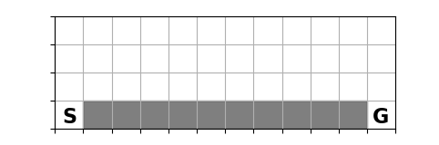
Figure 1: Cliff Walk Gridworld

In the “Absent Supervisor” gridworld environment (Figure 2) the objective is to reach the goal state by controlling four discrete actions up, down, left, right. The four center squares are impassable. For each episode a supervisor is absent or present with uniform probability. The state is encoded as a binary vector. The environment provides the agent a reward of -1 at each time step and a reward of +50 for entering the goal. When the supervisor is present the orange state, located immediately above the goal state, highlighted in Figure 2 provides a large negative reward (-30) but no such reward when the supervisor is absent. We would like the agent to never pass through the orange punishment state. The intent of the environment is to demonstrate that when provided the opportunity to cheat by passing through the orange state when the supervisor is absent traditional deep reinforcement learning algorithms will do so.

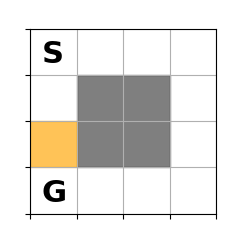
Figure 2: Absent Supervisor Gridworld

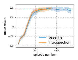
Figure 3: Episodes until “Lunar Lander” solved for DDQN (baseline) with and without Introspection Learning

In each case, the policy $\pi$ considered was a neural network with two hidden layers each having 32 nodes and hyperbolic tangent activations. The output activation was linear with one node for each action. DDQN with soft target network updates (?), the proportional variant of Prioritized Experience Replay(?), and an $\epsilon$ greedy exploration policy were employed to train the agent with the hyperparameters summarized in Table 1.

Hyperparameter	Value
experience replay every $n$ timesteps	2
replay buffer size	1e5
batch size	64
$\gamma$ (Discount factor)	0.99
$\alpha$ (Learning rate)	1e-3
$\tau$ (Soft target network update rate)	1e-2
PER $\alpha$ (TD error prioritization)	0.6
PER $\beta$ (Bias correction)	0.6

Table 1: DDQN hyperparameters used during training

In the “Lunar Lander” environment, the Introspection Learning parameters were set as follows. For the query schedule, we determine at what interval batches will be searched for and when searching for batches will cease and training will proceed as normal. We experimented with solving for state batches at a predetermined interval (every 100 episodes) and ceasing when the 100 episode moving average reward crossed a predetermined threshold. For training on state batches, states found were treated as terminal states with high negative reward (-100) as determined by the rules of the environment for terminal states. We have generally found that incorporating the state batches into the replay buffer is beneficial early in the learning process when the policy is poor, as it introduces bias (cf. (?)).The query constraints in both cases were to look for states whose $x$-coordinates were outside of the landing zone ($x<-0.25$ or $x>0.25$), such that the agent favors selecting an action that would result in it moving further away from from the landing zone.

This region of the state-space was divided into boxes using a simple quantization scheme that ignored regions of state space where examples satisfying the query constraints would be impossible to find. In general, such quantization schemes should be sufficiently fine-grained to allow generation of many and diverse examples. Twenty training runs with a set of twenty random seeds were run with and without our approach for a maximum of 500,000 timesteps. Results averaged over the training runs are summarized in Figure 3. DDQN with Introspection Learning solved the environment in a mean of 893 episodes while DDQN without Introspection Learning (baseline) failed to successfully solve the environment on average within 500,000 timesteps.

In addition to observing performance benefits, we also evaluated the agents trained with Introspection Learning for robustness benefits. In particular, we periodically stored the weights of both the Introspection Learning agent and the baseline agent during training for each of the twenty runs. We then recorded, for different regions of state space, statistics regarding the Sat, Unsat and Timeout results obtained when querying the SMT-solver on these agents across training. To recall, in this case, a Sat result indicates that there exists a state $s$ in the specified region $U$ of state space such that an undesirable action $\pi(s)$ (in this case, moving away from the landing zone) is selected by the agent. Likewise, an Unsat result indicates that there is a mathematical proof that there exists no state $s$ in $U$ such that $\pi(s)$ is undesirable. We gathered Sat, Unsat and Timeout data across a number of different selections of $U$. Tables 2 and 3 record the percentages of each kind of result across all twenty test runs that were captured at four points during training. The selection of $(U_{i})_{i}$ queried here were a subset of the subsets of (state,action)-space queried during the actual Introspection Learning training and the results show a clear improvement of robustness over the baseline. Timeouts during training were set to five seconds and to ten seconds during evaluation. One interesting point that we noticed in analyzing the robustness evaluation data is that larger numbers of Unsat results for the Introspection Learning agents were obtained at the beginning of training than the end. This is illustrated, for a typical example (the run with ID number 480951) in Figure 4. This is likely due to the schedule employed as part of the introspection learning algorithm and highlights the more general fact that reinforcement learning agents are sometimes subject to “forgetting” important learned behavior at later stages of training. Since the agents at the end of training were typically very good at solving the task, the regions of state space in which this forgetfulness would manifest themselves were likely off-trajectory (i.e., unreachable by the current policy).

In order to emphasize that this improvement is very much a function of the specific $(U_{i})_{i}$ used during training, and tested at evaluation time, we include for comparison in Table 4 the average percentages for an alternative selection of $(U_{i})_{i}$ used at evaluation time. Here the improvements are more modest.

Figure 4: Total number of unsat instances as a function of time for baseline (DDQN) and IL.

Run ID	Unsat	Sat	Timeout
34001	0%	62.5%	37.5%
390797	0%	100%	0%
747524	0%	75%	25%
480621	25%	50%	25%
475982	50%	25%	25%
319324	25%	62.5%	12.5%
449374	0%	50%	50%
491386	0%	50%	50%
532333	0%	50%	50%
55487	0%	75%	25%
4211	0%	50%	50%
480951	0%	100%	0%
219015	0%	87.5%	12.5%
481614	0%	75%	25%
367249	25%	50%	25%
508732	0%	100%	0%
521233	0%	50%	50%
543696	0%	75%	25%
998982	0%	100%	0%
36067	0%	75%	25%
Average	6.250%	68.125%	25.625%

Table 2: Percentages of Sat, Unsat and Timeout instances for Baseline DDQN at four points during training.

Run ID	Unsat	Sat	Timeout
34001	50%	25%	25%
390797	25%	25%	50%
747524	0%	50%	50%
480621	25%	0%	75%
475982	25%	50%	25%
319324	0%	75%	25%
449374	0%	50%	50%
491386	0%	45.8333%	54.1667%
532333	25%	25%	50%
55487	25%	50%	25%
4211	50%	25%	25%
480951	0%	75%	25%
219015	25%	37.50%	37.50%
481614	25%	75%	0%
367249	25%	75%	0%
508732	0%	75%	25%
521233	50%	50%	0%
543696	79.1667%	0%	20.8333%
998982	25%	33.3333%	41.6667%
36067	25%	0%	75%
Average	23.958%	42.083%	33.958%

Table 3: Percentages of Sat, Unsat and Timeout instances for Introspection Learning at four points during training.

Run ID	Unsat	Sat	Timeout
Baseline	83.3%	1.4%	15.3%
Introspection	85.3%	0.6%	14.2%

Table 4: Average percentages of Sat, Unsat and Timeout instances for Baseline DDQN versus Introspection Learning for the full batch of all twenty runs on another selection of query subsets $(U_{i})_{i}$. For this choice of subsets, the gains in robustness are more modest.

In the “Absent Supervisor” environment the Introspection Learning parameters were set as follows. Solving for state batches is unnecessary as in this discrete state environment we are only concerned with the agent choosing to enter the orange punishment state from the state directly above it. For the query schedule solving for this specific behavior is performed at every timestep and during training this transition is treated as terminal with high negative reward (-100). Results for DDQN with and without Introspection Learning are provided in Figures 5 and 6 respectively. One interesting point about the “Absent Supervisor” environment is that, for the evident notion of good policy, one of the hypotheses (the “Strong Compatiblity” assumption) of our Theorem 1 is violated.

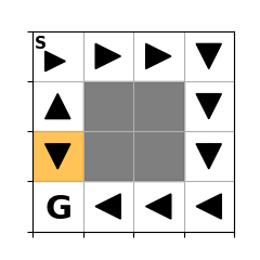
Figure 5: Final DDQN policy with Introspection Learning does not select to enter the orange punishment state when the supervisor is absent.

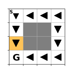
Figure 6: Final DDQN policy without Introspection Learning (baseline) selects to cheat and enter the orange punishment state when the supervisor is absent.

In the “Cliff Walk” environment the Introspection Learning parameters were set as follows. Solving for state batches is unnecessary as in this discrete state environment we are only concerned with the agent choosing to enter the cliff states which can only be done from the state directly above each cliff state respectively. For the query schedule solving for these specific behaviors is performed at every timestep and during training this transition is treated as terminal with high negative reward (-100). It should be noted that in this particular case the environment already treats these transitions as terminal with high negative reward (-100) and thus Introspection Learning will not alter the optimal policy (in particular, the hypotheses of Theorem 1 are satisfied). In this experiment, five training runs with a set of five random seeds were run with and without our approach until the environment was solved. During training, at each timestep, a running count was kept of the number of states from which the agent would select to enter the cliff states “lemming”. During training the policies were found to lemming on average 112 times with Introspection Learning and 29,501 times without. It was experimentally found that an agent with Introspection Learning would rarely learn a policy during training that would enter the cliff after the first training episode while it was routine for an agent without Introspection Learning. Representative policies learned by DDQN with and without Introspection Learning after 30 training episodes are provided in Figures 7 and 8 respectively. Additionally, agents with Introspection Learning enjoyed a small performance benefit solving the environment in 208 episodes on average over the five training runs while agents without Introspection Learning averaged 229 episodes to solve the environment.

Figure 7: Representative DDQN policy with Introspection Learning after 30 episodes of training has learned a safer policy of avoiding the cliff.

Figure 8: Representative DDQN policy without Introspection Learning (baseline) after 30 training episodes still selects to enter the cliff from some states.

5 Conclusions

In this paper we have introduced a novel reinforcement learning algorithm based on ideas coming from formal methods and SMT-solving. We have shown that, on suitable problems, these techniques can be employed in order to improve robustness of RL agents and to speed up their training. We have also given examples of how SMT-solving can be used to analyze reinforcement learning agent robustness. There are a number of extensions of this preliminary work possible. We mention several prominent directions here.

First, the focus here has been on single-step analysis of agent behavior, but a reachability analysis approach focused on trajectories leading to target states would likely generate more relevant data for learning. E.g., consider a geo-fenced space that we do not want the agent to enter and that is reachable through many different (state, action) combinations. Once a violation occurs, we would like to examine the trajectory in order to learn what earlier choices led the agent there.

Second, whereas in our “lunar lander” experiments we utilized an ad hoc quantization of the state space, it should be in many cases possible to learn such regions as part of the algorithm. This is a hard search problem so relying on these parameterizations is necessary and should therefore be automated. In conjunction with the reachability analysis mentioned above, this approach is likely to give more targeted and therefore useful data to include in the replay buffer.

Finally, while the SMT-solving technology being used is sufficient for low-dimensional state-spaces, these techniques face scalability issues on large state-spaces such as those coming from video data. How to handle these higher-dimensional state-spaces in a similar way is one of the exciting challenges in this area.

Acknowledgments

We would like to thank Ramesh S, Doug Stuart, Huafeng Yu, Sicun Gao, Aleksey Nogin, and Pape Sylla for useful conversations on topics related to this paper. We are also grateful to Tom Bui, Bala Chidambaram, Cem Saraydar, Roy Matic, Mike Daily and Son Dao for their support of and guidance regarding this research. Finally, we would like to thank Alessio Lomuscio and Clark Barrett for their interest in this work and for encouraging us to capture these results in a paper.

6 Appendix: Theoretical Results

Fix a pre-MDP $D$ and assume given a (non-empty) subset $\mathcal{G}$ of $\Pi(D)$ which we regard as the good policies: those policies $\pi$ whose $(s,\pi(s))$ have the properties of interest.

Definition 5.

MDPs $M$ and $M^{\prime}$ are equivalent whenever $\textnormal{Opt}(M)\subseteq\textnormal{Opt}(M^{\prime})$ and $\textnormal{Opt}(M^{\prime})\subseteq\textnormal{Opt}(M)$.

Furthermore, throughout this section we assume given a fixed MDP $M=(r,T)$ in $\mathcal{M}(D)$. Additionally, assume given a fixed discount factor $0\leq\gamma<1$. We also adopt throughout this section two further hypotheses, which we now describe.

Assumption 1 (Bad Set).

There exists a subset $B\subseteq S\times A$ such that $\pi$ is in $\mathcal{G}$ if and only if, for all $(s,a)\in B$, $\pi(s)\neq a$.

Our next hypothesis guarantees that the reward structure is already sufficiently compatible with $\mathcal{G}$.

Assumption 2 (Strong Compatibility).

All optimal policies for $M$ are in $\mathcal{G}$. I.e., $\textnormal{Opt}(M)\subseteq\mathcal{G}$.

We define a new MDP structure $M^{\dagger}=(r^{\dagger},T^{\dagger})$ in $\mathcal{M}(D)$ by

$$T^{\dagger} :=T\cup B,\text{ and}$$

$$r^{\dagger}(s,a) :=\begin{cases}-1+\min_{\pi}Q^{\pi}_{M}(s,a)&\text{ if }(s,a)\in B\text{, and}\\ r(s,a)&\text{ otherwise.}\end{cases}$$

It is straightforward to prove that $r^{\dagger}$ is bounded since $r$ is. Note that we are also modifying the underlying pre-MDP here by now imposing the condition that $a_{b}\colon s_{b}\to s_{t}$.

An immediate proof of the following proposition can be obtained using the notion of bounded corecursive algebra from (?), where it is shown that the state-value functions $V^{\pi}_{M}\colon S\to\mathbb{R}$ are canonically determined by the generating maps $v^{\pi}_{M}\colon S\to\mathbb{R}\times D(S)$ given by

$$v^{\pi}_{M}(s) :=(r(s,\pi(s)),p(s,\pi(s))),$$

where $D(-)$ is the probability distribution monad.

Proposition 1.

If $\pi$ is in $\mathcal{G}$, then $V^{\pi}_{M^{\dagger}}=V^{\pi}_{M}$.

Proof.

It suffices to show that $v^{\pi}_{M^{\dagger}}=v^{\pi}_{M}$, which is trivial for $\pi$ in $\mathcal{G}$. ∎

Corollary 1.

If $\pi$ is in $\mathcal{G}$, then $Q^{\pi}_{M^{\dagger}}(s,a)=Q^{\pi}_{M}(s,a)$ if and only if $(s,a)\notin B$.

Lemma 1.

$\textnormal{Opt}(M)\subseteq\textnormal{Opt}(M^{\dagger})$.

Proof.

Suppose given an optimal policy $\pi$ for $M$. By Bellman optimality, $\pi$ is optimal for $M^{\dagger}$ if and only if, for all $s$,

$$\pi(s)\in\operatorname*{arg\,max}_{a}Q^{\pi}_{M^{\dagger}}(s,a).$$

Let $s$ and $a$ be given. There are two cases depending on whether or not $(s,a)\in B$.

When $(s,a)\notin B$,

$$Q^{\pi}_{M^{\dagger}}(s,a) =Q^{\pi}_{M}(s,a)$$

$$\leq Q^{\pi}_{M}(s,\pi(s))$$

$$=Q^{\pi}_{M^{\dagger}}(s,\pi(s)),$$

where the equations are by Corollary 1 and the inequality is by optimality of $\pi$.

When $(s,a)\in B$,

$$Q^{\pi}_{M^{\dagger}}(s,a) =-1+\min_{\pi^{\prime}}Q^{\pi^{\prime}}_{M}(s,a)+0$$

$$\leq-1+Q^{\pi}_{M}(s,a)$$

$$<Q^{\pi}_{M}(s,a)$$

$$\leq Q^{\pi}_{M}(s,\pi(s))$$

$$=Q^{\pi}_{M^{\dagger}}(s,\pi(s)),$$

where the final inequality is by optimality of $\pi$ and the final equality is by Corollary 1. ∎

Lemma 2.

$\textnormal{Opt}(M^{\dagger})\subseteq\mathcal{G}$.

Proof.

Let a policy $\pi$ for $M^{\dagger}$ be given such that, for some $s$, $(s,\pi(s))\in B$ and let $\pi^{\prime}$ be an optimal policy for $M$. Then

$$Q^{\pi}_{M^{\dagger}}(s,\pi(s)) <Q^{\pi}_{M}(s,\pi(s))$$

$$\leq Q^{\pi^{\prime}}_{M}(s,\pi^{\prime}(s))$$

$$=Q^{\pi^{\prime}}_{M^{\dagger}}(s,\pi^{\prime}(s)),$$

so that such a $\pi$ cannot be optimal. ∎

Theorem 1.

$M$ and $M^{\dagger}$ are equivalent.

Proof.

By Lemma 1 it suffices to show that $\textnormal{Opt}(M^{\dagger})\subseteq\textnormal{Opt}(M)$, which is immediate since

$$V^{\pi}_{M}=V^{\pi}_{M^{\dagger}}=V^{\pi^{\prime}}_{M^{\dagger}}=V^{\pi^{\prime}}_{M},$$

for any optimal policy $\pi$ for $M^{\dagger}$ and any optimal policy $\pi^{\prime}$ for $M$. Here the first equation is by Proposition 1 and Lemma 2, the second equation is by optimality of $\pi^{\prime}$ for $M^{\dagger}$ by Lemma 1, and the final equation is by Proposition 1 and the Strong Compatibility hypothesis. ∎

Alessio

References

- [1] Peter Abbeel and Andrew Y. Ng “Apprenticeship Learning via Inverse Reinforcement Learning” In Proceedings of the 21st International Conference on Machine Learning, 2004
- [2] Brandon Amos and J. Kolter “OptNet: Differentiable Optimization as a Layer in Neural Networks”, 2017 arXiv: http://arxiv.org/abs/1703.00443
- [3] “dReal: an SMT solver for nonlinear theories over the reals” In CADE, 2013
- [4] Frank M.. Feys, Helle Hvid Hansen and Lawrence S. Moss “Long-Term Values in Markov Decision Processes, (co)algebraically” In IFIP International Federation for Information Processing 2018 11202, Lecture Notes in Computer Science Springer, 2018, pp. 78–99
- [5] S. Gao, J. Avigad and E.. Clarke “Delta-Decidability over the reals” In Proceedings of the 27th Annual ACM/IEEE Symposium on Logic in Computer Science (LICS), 2012
- [6] Amy Greenwald and Keith Hall “Correlated-Q Learning” URL: https://www.aaai.org/Papers/ICML/2003/ICML03-034.pdf
- [7] Hado Hasselt, Arthur Guez and David Silver “Deep Reinforcement Learning with Double Q-learning” In Proceedings AAAI, 2016 arXiv: http://arxiv.org/abs/1509.06461
- [8] Guy Katz et al. “Reluplex: An efficient SMT solver for verifying deep neural networks” In CAV 2017, 2017 URL: https://arxiv.org/abs/1702.01135
- [9] Jan Leike et al. “AI Safety Gridworlds”, 2017 URL: https://deepmind.com/research/publications/ai-safety-gridworlds/
- [10] Timothy P. Lillicrap et al. “Continuous control with deep reinforcement learning”, 2015 arXiv: http://arxiv.org/abs/1509.02971
- [11] Michael L. Littman “Markov Games as a Framework for Multi-Agent Reinforcement Learning” In In Proceedings of the Eleventh International Conference on Machine Learning
- [12] Alessio Lomuscio and Lalit Maganti “An approach to reachability analysis for feed-forward ReLU neural networks”, 2017 URL: https://arxiv.org/abs/1706.07351
- [13] Andrew Y. Ng and Stuart J. Russell “Algorithms for Inverse Reinforcement Learning” In ICML ’00 Proceedings of the Seventeenth International Conference on Machine Learning, 2000, pp. 663–670
- [14] OpenAI “OpenAI Gym Website”, 2018 URL: https://gym.openai.com
- [15] Tu-Hoa Pham, Giovanni De Magistris and Ryuki Tachibana “OptLayer - Practical Constrained Optimization for Deep Reinforcement Learning in the Real World”, 2017 arXiv: http://arxiv.org/abs/1709.07643
- [16] Tom Schaul, John Quan, Ioannis Antonoglou and David Silver “Prioritized Experience Replay”, 2015 arXiv: http://arxiv.org/abs/1511.05952
- [17] Richard S. Sutton and Andrew G. Barto “Reinforcement Learning: An Introduction” MIT Press, 2018