Rate-independent evolution of sets

Abstract

The goal of this work is to analyze a model for the rate-independent evolution of sets with finite perimeter. The evolution of the admissible sets is driven by that of a given time-dependent set, which has to include the admissible sets and hence is to be understood as an external loading. The process is driven by the competition between perimeter minimization and minimization of volume changes.

In the mathematical modeling of this process, we distinguish the adhesive case, in which the constraint that the (complement of) the ‘external load’ contains the evolving sets is penalized by a term contributing to the driving energy functional, from the brittle case, enforcing this constraint. The existence of Energetic solutions for the adhesive system is proved by passing to the limit in the associated time-incremental minimization scheme. In the brittle case, this time-discretization procedure gives rise to evolving sets satisfying the stability condition, but it remains an open problem to additionally deduce energy-dissipation balance in the time-continuous limit. This can be obtained under some suitable quantification of data. The properties of the brittle evolution law are illustrated by numerical examples in two space dimensions.

Dedicated to Alexander Mielke on the occasion of his 60th birthday

MSC 2010.

35A15, 35R37, 49Q10, 74R10.

Keywords and phrases.

Unidirectional evolution of sets by competition of perimeter and volume, minimizers of perimeter perturbed by a nonsmooth functional, Minimizing Movements, stability, Energetic solutions.

1 Introduction

The aim of this work is to introduce and analyze a notion of rate-independent evolution for a set-valued function $Z:[0,T]\rightrightarrows\Omega$ (with $\Omega$ a bounded domain in $\mathbb{R}^{d}$), whose evolution is triggered by that of another, given set-valued function $F:[0,T]\rightrightarrows\Omega$, in the position of an external force, through the constraint

$$Z(t)\cap F(t)=\emptyset\quad\text{for every }t\in[0,T].$$ (1.1)

The evolution of $Z$ is additionally ruled by the competition between the minimization of the perimeter and that of volume changes.

Related models: brittle delamination and adhesive contact

Our study is inspired and motivated by the modeling of delamination between two (elastic) bodies $O_{+}$ and $O_{-}\subset\mathbb{R}^{m}$, bonded along a prescribed contact surface $\Gamma=\overline{O}_{+}\cap\overline{O}_{-}$ over time interval $(0,T)$. Following the approach by M. Frémond [Fré88, Fré02], this process can be described in terms of the temporal evolution of a phase-field type parameter, the delamination variable $z:(0,T)\times\Gamma\to[0,1]$, which represents the fraction of fully effective molecular links in the bonding. Therefore, $z(t,x)=1$ ($z(t,x)=0$, respectively) means that the bonding is fully intact (completely broken) at a given time instant $t\in[0,T]$ and in a given material point $x\in\Gamma$. In models for brittle delamination, the evolution of $z$ is coupled to that of the (small-strain) displacement variable $u:(0,T)\times O\to\mathbb{R}^{m}$ (with $O:=O_{+}\cup O_{-}$) through the so-called

$$\text{brittle constraint}\qquad z\mathchoice{\big{[}\big{[}u\big{]}\big{]}}{[[u]]}{[\![u]\!]}{[\![u]\!]}=0\quad\text{a.e.\ in }(0,T)\times\Gamma.$$ (1.2)

In (1.2), $\mathchoice{\big{[}\big{[}u\big{]}\big{]}}{[[u]]}{[\![u]\!]}{[\![u]\!]}=u^{+}|_{\Gamma}-u^{-}|_{\Gamma}$ ($u^{+},\,u^{-}$ denoting the restrictions of $u$ to $O_{+},\,O_{-}$, respectively) is the jump of $u$ across the interface $\Gamma$. Therefore, (1.2) ensures the continuity of the displacements, i.e. $\mathchoice{\big{[}\big{[}u\big{]}\big{]}}{[[u]]}{[\![u]\!]}{[\![u]\!]}=0$, in the (closure of the) set of points where (a portion of) the bonding is still active, i.e. $z>0$. In fact, (1.2) allows for displacement jumps only at points where the bonding is completely broken, namely where $z=0$. The set $\Gamma\setminus\mathop{\mathrm{supp}}(z)$, where the displacements may jump, can be thus understood as a crack set; indeed, brittle delamination can be interpreted as a model for brittle fracture, along a prescribed $(m{-}1)$-dimensional surface.

To the best of our knowledge, the analysis of the above described brittle delamination model has been carried out only in the case this process is treated as rate-independent. Namely, the evolution of the internal variable, responsible for the dissipation of energy, is governed by a dissipation potential ${\mathcal{R}}$ which is positively homogeneous of degree $1$, i.e. fulfilling ${\mathcal{R}}(\lambda\dot{z})=\lambda{\mathcal{R}}(\dot{z})$ for all $\lambda\geq 0$. In that case, the process can be mathematically modeled by means of the general concept of Energetic solution to a rate-independent system, pioneered in [MT99, MT04] (cf. also the parallel notion of quasistatic evolution for brittle fracture, [FM98, DMT02]). The existence of Energetic solutions to the brittle delamination system was proven in [RSZ09] by passing to the limit, as the penalization parameter $k$ blows up, in the Energetic formulation for an approximate system. Therein, the brittle constraint (1.2) was indeed penalized by the

$$\text{adhesive contact term}\qquad\int_{\Gamma}kz|\mathchoice{\big{[}\big{[}u\big{]}\big{]}}{[[u]]}{[\![u]\!]}{[\![u]\!]}|^{2}\,\mathrm{d}\mathcal{H}^{m-1}(x),\qquad k\in(0,\infty)$$ (1.3)

contributing to the driving energy. For the corresponding rate-independent system, referred to as adhesive contact system, the existence of Energetic solution dates back to [KMR06]. The passage from adhesive to brittle was also studied in [RT15] by extending the existence of Energetic solutions to the case in which the rate-independent evolution of the delamination parameter $z$ is coupled to the rate-dependent evolution of the displacement, ruled by a (no longer quasi-static) momentum balance with viscosity. In order to overcome the analytical difficulties attached to the coupling of rate-independent/rate-dependent behavior, in [RT15] a gradient regularization is advanced for the delamination variable of $\mathrm{BV}$-type. In fact, (1) the constraint $z\in\{0,1\}$ was added to the model, making it closer to Griffith-type model for crack evolution; (2) the term $|\mathrm{D}z|(\Gamma)$ (namely, the total variation of the measure $\mathrm{D}z$) was added to the driving energy functional. Since $z$ is the characteristic function of the set $Z:=\{x\in\Gamma\,:\ z(x)>0\}$, the gradient regularization $|\mathrm{D}z|(\Gamma)$ coincides with the perimeter $P(Z,\Gamma)$ of $Z$ in $\Gamma.$

The rate-independent evolution of sets $Z:[0,T]\rightrightarrows\Omega$ studied in this paper can be understood as an abstraction of the delamination process addressed in [RSZ09, RT15]. Indeed, suppose that $\Omega=\Gamma$, and that the temporal evolution of the set

$$F(t):=\{x\in\Gamma_{\mbox{\tiny\rm C}}\,:\ \mathchoice{\big{[}\big{[}u(t,x)\big{]}\big{]}}{[[u(t,x)]]}{[\![u(t,x)]\!]}{[\![u(t,x)]\!]}\neq 0\}$$ (1.4)

is given. The sets $Z(t)$ correspond to the supports of the delamination variable and, when the set-valued mapping $F:[0,T]\rightrightarrows\Omega$ is given by (1.4), (1.1) renders the brittle constraint (1.2). Therefore, hereafter we shall refer to (1.1) as a (generalized) brittle constraint, too. Like in [RT15], the energy functional driving the evolution of the sets $Z$ will feature their perimeter $P(Z,\Omega)$ in $\Omega$. Again in analogy with delamination processes, in addition to the brittle case, in which (1.1) is enforced, we will also address the adhesive case, in which (1.1) is suitably penalized.

Our aim is threefold:

1. prove the existence of Energetic solutions for both the adhesive and the brittle evolution of sets;

2. investigate to what extent the fine geometric properties proved in [RT15] for (the supports of) Energetic solutions to the adhesive and brittle delamination systems, carry over to this generalized setting;

3. gain insight into the connection between this rate-independent evolution of sets, and the well-known mean curvature flow.

Solution concepts and our existence results

Throughout the paper, we will work under the (additional, w.r.t. the delamination case (1.4)) assumption that the ‘external load’ $F:[0,T]\rightrightarrows\Omega$ is monotonically increasing, namely

$$F(s)\subset F(t)\qquad\text{ for all $0\leq s\leq t\leq T$.}$$ (1.5)

Hence, in view of the constraint $Z(t)\subset F^{c}(t)$ from (1.1), it will be natural to enforce for the set function $Z:[0,T]\rightrightarrows\Omega$ the opposite monotonicity property, viz. $Z(t)\subset Z(s)$ for all $0\leq s\leq t\leq T$.

The adhesive and the brittle processes will be mathematically modeled by a triple $(\mathbf{Z},{\mathcal{E}}_{k},{\mathcal{D}})_{k}$, $k\in\mathbb{N}\cup\{\infty\}$, with

• $\mathbf{Z}=\{Z\subset\Omega\,:\ {\mathcal{L}}^{d}(Z)<\infty\}$ the state space;

• the driving energy functional

  $${\mathcal{E}}_{\infty}(t,Z):=P(Z,\Omega)+{\mathcal{J}}_{\infty}(t,Z)\qquad\text{with }{\mathcal{J}}_{\infty}(t,Z):=\begin{cases}0&\text{ if }Z\cap F(t)=\emptyset,\\ \infty&\text{ otherwise},\end{cases}$$

  for the brittle process, while for the adhesive process we will pose

  $${\mathcal{E}}_{k}(t,Z):=P(Z,\Omega)+{\mathcal{J}}_{k}(t,Z)\,,\qquad\text{where the term }{\mathcal{J}}_{k}(t,Z):=\int_{\Omega}kf(t)\chi_{Z}\,\mathrm{d}x,\ k\in(0,\infty),$$

  penalizes the brittle constraint (1.1), in that the support of the function $f(t)$ coincides with $F(t)$;

• the dissipation (quasi-)distance

  $${\mathcal{D}}:\mathbf{Z}\times\mathbf{Z}\to[0,\infty],\quad{\mathcal{D}}(Z_{1},Z_{2}):=\left\{\begin{array}[]{ll}a{\mathcal{L}}^{d}(Z_{1}\setminus Z_{2})&\text{if }Z_{2}\subset Z_{1},\\ \infty&\text{otherwise}\end{array}\right.$$

  for some $a>0$, enforcing that $Z:[0,T]\rightrightarrows\Omega$ is monotonically decreasing.

We will investigate the existence of Energetic solutions to the rate-independent systems $(\mathbf{Z},{\mathcal{E}}_{k},{\mathcal{D}})_{k}$, $k\in\mathbb{N}\cup\{\infty\}$, namely functions $Z:[0,T]\rightrightarrows\Omega$ complying with

• the global stability condition

  $${\mathcal{E}}_{k}(t,Z(t))\leq{\mathcal{E}}_{k}(t,\widetilde{Z})+{\mathcal{D}}(Z(t),\widetilde{Z})\quad\text{for all }\widetilde{Z}\in\mathbf{Z},\quad\text{for all }t\in[0,T],$$ (1.6)

• the energy-dissipation balance

  $${\mathcal{E}}_{k}(t,Z(t))+\mathrm{Var}_{{\mathcal{D}}}(Z;[0,t])={\mathcal{E}}_{k}(0,Z(0))+\int_{0}^{t}\partial_{t}{\mathcal{E}}_{k}(s,Z(s))\,\mathrm{d}t\quad\text{for all }t\in[0,T].$$ (1.7)

  In (1.7), $\mathrm{Var}_{{\mathcal{D}}}(Z;[0,t])$ is the total variation functional induced by the dissipation distance ${\mathcal{D}}$, cf. (2.13) below, and the power functional $\partial_{t}{\mathcal{E}}_{k}$ has to be suitably understood in the brittle case $k=\infty$, in which the mapping $t\mapsto{\mathcal{E}}_{\infty}(t,Z)$ ceases to be smooth, see (2.18) below.

As a matter of fact, the derivative-free character of the Energetic concept makes it suitable to formulate evolutions, like ours, set up in spaces lacking a linear or even a metric structure, cf. e.g. the aforementioned pioneering work [DMT02] on brittle fractures, [MM05] for rate-independent processes in general topological spaces, and [BBL08] for the rate-independent evolution of debonding membranes.

With our first main result, Theorem 4.5, we establish the existence of Energetic solutions for the rate-independent system $(\mathbf{Z},{\mathcal{E}}_{k},{\mathcal{D}})_{k}$ in the adhesive case $k<\infty$. Its proof will be carried out by proving that (the piecewise constant interpolants $(\overline{Z}_{\kern-1.0pt\tau})_{\tau}$ of) the discrete solutions $(Z_{\tau}^{i})$ of the associated time-incremental minimization scheme, namely

$$Z_{\tau}^{i}\in\mathop{\mathrm{Argmin}_{Z\in\mathbf{Z}}}\big{\{}{\mathcal{E}}_{k}(\mathsf{t}^{i}_{\tau},Z)+{\mathcal{D}}(Z^{i-1}_{\tau},Z)\big{\}}$$ (1.8)

(where $\Pi_{\tau}:=\{\mathsf{t}^{0}_{\tau}=0<\mathsf{t}^{1}_{\tau}<\ldots,<\mathsf{t}^{N}_{\tau}=T\}$ is a partition of the time interval $(0,T)$ with step size $\tau$), do converge to an Energetic solution of the adhesive system as $\tau\downarrow 0$. For this, we will pass to the limit in the discrete versions of the stability condition, and of the upper energy-dissipation estimate $\leq$, to obtain their analogues on the time-continuous level.

The situation for the brittle system is more involved, essentially due to the intrinsically nonsmooth character of the brittle constraint (1.1). This brings about a nonsmooth time dependence $t\mapsto{\mathcal{E}}_{\infty}(t,Z)$ that has to be handled with suitable arguments, since most of the techniques for treating the Energetic formulation of rate-independent systems rely on the condition that the driving energy functional is at least absolutely continuous w.r.t. time, cf. also Remark 2.1 ahead. In our specific case, because of (1.1) we are no longer in a position to show that the discrete solutions to (1.8) satisfy a discrete upper energy estimate. Therefore, it remains an open problem to prove the existence of Energetic solutions by passing to the time-continuous limit in scheme (1.8).

Nonetheless, time incremental minimization yields the existence of limiting curves satisfying the stability condition (1.6). With a terminology borrowed from the theory of gradient flows [AGS08], we have chosen to qualify such curves as Stable Minimizing Movements, cf. Definition 2.3 ahead. Then, Theorem 4.1 asserts the existence of Stable Minimizing Movements both in the adhesive case $k\in\mathbb{N}$ and in the brittle case $k=\infty$.

The concept of Stable Minimizing Movement, though definitely weaker than the Energetic solution notion, seems to be relevant as well. On the one hand, it is tightly related to time discretization scheme (1.8), and it is on the level of (1.8) that we can compare our rate-independent evolution with the mean curvature flow, see Remark 2.6. On the other hand, Stable Minimizing Movements enjoy the very same fine properties as those proved in [RT15] for the (semi-)stable delamination variables for the adhesive contact and brittle delamination systems. Namely, the sets $Z$ fulfill a lower density estimate, which prevents outward cusps, cf. Proposition 4.3. Further geometric properties of Stable Minimizing Movements are discussed in Section 4.1.

As previously mentioned, Thm.  4.5 will show that, for $k\in\mathbb{N}$ Stable Minimizing Movements enhance to Energetic solutions. Finally, Theorem 4.6 will provide an existence result for the brittle system. Namely, we will identify a special setting in which the Energetic solutions $(Z_{k})_{k}$ of the adhesive systems $(\mathbf{Z},{\mathcal{E}}_{k},{\mathcal{D}})$, $k\in\mathbb{N},$ approximate an Energetic solution of the brittle one $(\mathbf{Z},{\mathcal{E}}_{\infty},{\mathcal{D}})$ as $k\to\infty$. In this case, we will find that the force term $\int_{0}^{T}\partial_{t}{\mathcal{E}}_{k}(t,Z_{k}(t))\,\mathrm{d}t$ tends to $0$ as $k\to\infty,$ and thus vanishes for the limit system.

Plan of the paper.

In Section 2 we fix the setup for the adhesive and brittle evolution of sets, and introduce Stable Minimizing Movements and Energetic solutions for both processes. In Section 3 we gain further insight into the time incremental minimization scheme (1.8); for its solutions we derive a priori estimates, and discrete versions of the stability condition and of the energy-dissipation inequality. Section 4 contains the statements of all of our existence results, as well as a detailed discussion on the properties of Stable Minimizing Movements, including some illustrative numerical experiments in two space dimensions in the brittle case. Theorems 4.1, 4.5, and 4.6 are then proved in Section 5.

Acknowledgements.

We are very grateful for all the discussions we have shared with Alexander Mielke about rate-independent systems, general mathematical questions, and far beyond. We wish him all the best for the next 60 years with a lot of creative thoughts, and the time to enjoy and elaborate on them. We are already looking forward to be part of this process!

Last but not least, the authors also want to acknowledge financial support: M.T. acknowledges the support through the DFG within the project “Reliability of efficient approximation schemes for material discontinuities described by functions of bounded variation” in the priority programme SPP 1748 ”Reliable Simulation Techniques in Solid Mechanics. Development of Nonstandard Discretisation Methods, Mechanical and Mathematical Analysis”. R.R. has been partially supported by a GNAMPA (INDAM) project. U.S.  acknowledges support by the Vienna Science and Technology Fund (WWTF) through Project MA14-009 and by the Austrian Science Fund (FWF) projects F 65, P 27052, and I 2375.

2 Setup and notions of solutions

First of all, in the upcoming Section 2.1 we fix the setting in which the notion of Energetic solution for the adhesive and brittle evolution of sets can be given. As mentioned in the Introduction, along with Energetic solutions we will also address the much weaker concept of Stable Minimizing Movement, which originates from the time-incremental minimization schemes for the adhesive and brittle systems. We shall set up these schemes, precisely introduce our solution notions, and compare our notion of evolution to the mean curvature flow, in Section 2.2 ahead.

2.1 Setup

Throughout this work, $\Omega\subset\mathbb{R}^{d}$ is a bounded (Lipschitz) domain. The evolution of sets studied in this paper is driven by a time-dependent function with values in the subsets of $\Omega$, $F:[0,T]\rightrightarrows\Omega$. We will denote by $F^{c}(t)=\Omega\backslash F(t)$ the complement of the set $F(t)$ and impose on the mapping $F$ the following conditions, that also involve a function $f:(0,T)\times\Omega\to\mathbb{R}$, suitably related to $F$:

$$F(t)\text{ is open for every }t\in[0,T];$$ (2.1a)

$$F(s)\subset F(t)\quad\text{for every }0\leq s\leq t\leq T$$ (2.1b)

$$\begin{aligned} &\exists\,f\in W^{1,1}(0,T;L^{1}(\Omega))\quad\text{such that }\text{for a.a.}\,t\in(0,T)\\ &f(t,\cdot)\geq 0\text{ a.e.\ in }\Omega\,\text{ and }\,F(t)=\{x\in\Omega\,:\ f(t,x)>0\}\,.\end{aligned}$$ (2.1c)

Remark 2.1.

Condition (2.1c) will ensure, for the energy functional ${\mathcal{E}}_{k}$ for the adhesive system (cf. (2.14a) ahead), that ${\mathcal{E}}_{k}(\cdot,Z)\in W^{1,1}(0,T)$. This property can be considered as ‘standard’ within the analysis of rate-independent systems, cf. [MR15]. We will rely on it, for instance, in the proof of the existence of Energetic solutions in the adhesive case, in order to readily conclude the energy-dissipation balance once the energy-dissipation upper estimate and the stability conditions have been verified, cf. the proof of Thm. 4.5 ahead.

However, even under (2.1c), for the brittle system the energy functional ${\mathcal{E}}_{\infty}$ (2.16a) fails to be differentiable w.r.t. time, due to the intrinsically nonsmooth character of the brittle constraint (1.1). One way to handle a nonsmooth time-dependence of the driving energy would be to resort to techniques based on the Kurzweil integral, cf. [KL09] and the references therein. In the case of our brittle system, though, we will avoid using these sophisticated tools. Essentially, the (somehow) simplified structure of the energy-dissipation balance will allow us to develop ad-hoc arguments in the proof of the existence of Energetic solutions to the brittle system.

We now introduce the notation for the state spaces that will enter in our solution concepts for the rate-independent evolution of sets:

$$\mathbf{Z} := \{Z\in\mathscr{L}(\Omega)\,:\,{\mathcal{L}}^{d}(Z)<\infty\}=\mathscr{L}(\Omega)\,,$$ (2.2a)

$$\mathbf{X} := \{Z\in\mathscr{L}(\Omega)\,:\,P(Z,\Omega)<\infty\}\,,$$ (2.2b)

where $\mathscr{L}(\Omega)$ denotes the $\sigma$-algebra of Lebesgue-measurable sets, while ${\mathcal{L}}^{d}(Z)$ is the Lebesgue measure of the set $Z$ in $\mathbb{R}^{d}$, and $P(Z,\Omega)$ its perimeter in $\Omega$.

Since the volume measure ${\mathcal{L}}^{d}$ and the perimeter $P$ are insensitive to null sets, all of our statements will be intended up to null sets. Moreover, we will identify sets $Z$ from $\mathbf{Z}$ with the functions $z:\Omega\to\{0,1\}$ such that $\chi_{Z}=z$, and indeed we will often use both notations, even within the same line. We recall that

$$P(Z,\Omega)=\sup\left\{\int_{\Omega}z\,\mathrm{div}(\varphi)\,:\ \varphi\in\mathrm{C}_{\mathrm{c}}^{1}(\Omega;\mathbb{R}^{d}),\ \|\varphi\|_{L^{\infty}}\leq 1\right\}=|\mathrm{D}z|(\Omega),$$ (2.3)

($\mathrm{C}_{\mathrm{c}}^{1}(\Omega;\mathbb{R}^{d})$ denoting the space of compactly supported $\mathrm{C}^{1}$-functions on $\Omega$). Hence $P(Z,\Omega)<\infty$ if and only if $z=\chi_{Z}$ has bounded variation on $\Omega$, i.e. $z\in\mathrm{SBV}(\Omega;\{0,1\})$, since its distributional derivative $\mathrm{D}z$ has no Cantor part. The state spaces for functions corresponding to $\mathbf{Z}$ and $\mathbf{X}$ are thus

$$L^{1}(\Omega)\quad\text{ and }\quad\mathrm{SBV}(\Omega;\{0,1\}):=\{z:\Omega\to\{0,1\}\text{ is the characteristic function of }Z\in\mathbf{X}\}\,.$$ (2.4)

Throughout this paper, we will employ the following notion of convergence of sets: we will say that a sequence of sets $(Z_{k})_{k}\subset\mathbf{X}$ converges weakly^∗ in $\mathbf{X}$ to a limit set $Z,$ if for their respective characteristic functions $z_{k}:=\chi_{Z_{k}}$ and $z:=\chi_{Z}$, there holds weak^∗-convergence in $\mathrm{SBV}(\Omega;\{0,1\}),$ i.e.,

$$Z_{k}\overset{*}{\rightharpoonup}Z\text{ in }\mathbf{X}\quad\Leftrightarrow\quad z_{k}\overset{*}{\rightharpoonup}z\quad\text{ in }\mathrm{SBV}(\Omega;\{0,1\})\,.$$ (2.5)

Both for the adhesive and the brittle systems we will consider the dissipation distance

$${\mathcal{D}}:\mathbf{Z}\times\mathbf{Z}\to[0,\infty],\quad{\mathcal{D}}(Z_{1},Z_{2}):=\left\{\begin{array}[]{ll}a{\mathcal{L}}^{d}(Z_{1}{\setminus}Z_{2})&\text{if }Z_{2}\subset Z_{1},\\ \infty&\text{otherwise}\end{array}\right.$$ (2.8)

for a constant $a>0$. For later use, we will also consider the corresponding dissipation distance (and denote it in the same way) on the space of characteristic functions, namely

$${\mathcal{D}}:L^{1}(\Omega)\times L^{1}(\Omega)\to[0,\infty],\quad{\mathcal{D}}(z_{1},z_{2}):=\left\{\begin{array}[]{ll}a(z_{1}-z_{2})&\text{if }z_{2}\leq z_{1}\quad\text{a.e.\ in }\Omega,\\ \infty&\text{otherwise.}\end{array}\right.$$ (2.11)

Clearly, (2.8) makes the evolution of a solution $Z$ to the adhesive/brittle system unidirectional, namely $Z:[0,T]\to\mathbf{Z}$ is nonincreasing:

$$Z(t)\subset Z(s)\quad\text{if }0\leq s\leq t\leq T.$$ (2.12)

In turn, by this monotonicity property we have that

$$\mathrm{Var}_{{\mathcal{D}}}(Z;[0,t]) :=\sup\left\{\sum_{j=1}^{M}{\mathcal{D}}(Z(\sigma_{j-1}),Z(\sigma_{j}))\,:\ 0=\sigma_{0}<\sigma_{1}<\ldots<\sigma_{M-1}<\sigma_{M}=t\right\}$$ (2.13)

$$={\mathcal{D}}(Z(0),Z(t))\,.$$

The evolution of the adhesive system will be driven by the energy functional

$${\mathcal{E}}_{k}:[0,T]\times\mathbf{X}\to[0,\infty)\,,\quad{\mathcal{E}}_{k}(t,Z):=P(Z,\Omega)+{\mathcal{J}}_{k}(t,Z)\quad\text{for }k\in\mathbb{N}\,,$$ (2.14a)

where the functional $${\mathcal{J}}_{k}:[0,T]\times\mathbf{Z}\to[0,\infty]$$ penalizes the “brittle constraint” (1.1), namely

$${\mathcal{J}}_{k}(t,Z):=\int_{\Omega}kf(t)z\,\mathrm{d}x\quad\text{for all }(t,Z)\in[0,T]\times\mathbf{Z},\qquad\text{for }k\in\mathbb{N}\,,$$ (2.14b)

where $$z\in L^{1}(\Omega) Z z=\chi_{Z}$$ is associated with via .

It is immediate to check that ${\mathcal{E}}_{k}$ is differentiable w.r.t. time at every $(t,Z)\in[0,T]\times\mathbf{Z}$, with

$$\partial_{t}{\mathcal{E}}_{k}(t,Z)=\int_{\Omega}k\partial_{t}f(t,x)z(x)\,\mathrm{d}x\quad\text{for all }(t,Z)\in[0,T]\times\mathbf{Z}.$$ (2.15)

In fact, thanks to (2.1c) we have that ${\mathcal{E}}_{k}(\cdot,Z)\in W^{1,1}(0,T)$ for all $Z\in\mathbf{Z}$. With slight abuse of notation, we will sometimes write ${\mathcal{E}}_{k}(t,z)$ (with $P(Z,\Omega)$ rewritten in terms of (2.3)), in place of ${\mathcal{E}}_{k}(t,Z)$.

The energy functional for the brittle system is

$${\mathcal{E}}_{\infty}:[0,T]\times\mathbf{X}\to[0,\infty]\,,\quad{\mathcal{E}}_{\infty}(t,Z):=P(Z,\Omega)+{\mathcal{J}}_{\infty}(t,Z)$$ (2.16a)

with $${\mathcal{J}}_{\infty}:[0,T]\times\mathbf{Z}\to[0,\infty]$$ the indicator functional associated with the constraint (1.1), i.e.

$${\mathcal{J}}_{\infty}(t,Z):=\begin{cases}0&\text{ if }Z\cap F(t)=\emptyset,\\ \infty&\text{ otherwise}.\end{cases}$$ (2.16b)

Since $F^{c}(t)=\{x\in\Omega\,:\,f(t,x)=0\}$, we have that $Z\subset F^{c}(t)$ if and only if $z=\chi_{Z}$ fulfills $z(x)f(t,x)=0$ (a.e. in $\Omega$). All in all, we have that

$${\mathcal{J}}_{\infty}(t,Z)=\begin{cases}0&\text{ if }z(x)f(t,x)=0\quad\text{for a.a.}\,x\in\Omega,\\ \infty&\text{ otherwise.}\end{cases}$$ (2.17)

In fact, also for the brittle system we will sometimes write ${\mathcal{J}}_{\infty}$ and ${\mathcal{E}}_{\infty}$ as functions of $(t,z)$ through the representation $z=\chi_{Z}$. In place of the usual power functional $\partial_{t}{\mathcal{E}}_{\infty}$, in this case only the left partial time derivative $\partial_{t}^{-}{\mathcal{E}}_{\infty}$ is well defined and fulfills

$$\partial_{t}^{-}{\mathcal{E}}_{\infty}(t,Z):=\lim_{h\uparrow 0}\frac{{\mathcal{E}}_{\infty}(t+h,Z)-{\mathcal{E}}_{\infty}(t,Z)}{h}=\lim_{h\uparrow 0}\frac{{\mathcal{J}}_{\infty}(t+h,Z)-{\mathcal{J}}_{\infty}(t,Z)}{h}=0\quad\forall\,(t,Z)\in\mathrm{dom}({\mathcal{E}}_{\infty})\,.$$ (2.18)

Indeed, ${\mathcal{E}}_{\infty}(t,Z)<\infty$ if and only if ${\mathcal{J}}_{\infty}(t,Z)=0$, i.e. $Z\cap F(t)=\emptyset$. Since $F:[0,T]\rightrightarrows\Omega$ is increasing with respect to time, we then have that $Z\cap F(t+h)=\emptyset$, i.e. ${\mathcal{J}}_{\infty}(t+h,Z)=0$, for all $h\in[-t,0)$, which gives (2.18). Let us stress that the monotonicity property (2.1b) plays a crucial role in ensuring that $\partial_{t}^{-}{\mathcal{E}}_{\infty}$ is well defined.

2.2 Stable Minimizing Movements and Energetic solutions for the adhesive and brittle systems

Time-incremental minimization.

We consider a partition $\Pi_{\tau}:=\{\mathsf{t}^{0}_{\tau}=0<\mathsf{t}^{1}_{\tau}<\ldots,<\mathsf{t}^{N}_{\tau}=T\},$ of the time interval $(0,T)$ with step size $\tau=\max_{i=1,\ldots,N_{\tau}}(\mathsf{t}^{i}_{\tau}{-}\mathsf{t}_{\tau}^{i-1})$. Discrete solutions arise from solving the time-incremental minimization problem: starting from $Z_{\tau}^{0}:=Z_{0}$ for a given $Z_{0}\in\mathbf{X}$, for every $i=1,\ldots,N_{\tau}$ find

$$Z_{\tau}^{i}\in\mathop{\mathrm{Argmin}_{Z\in\mathbf{X}}}\big{\{}{\mathcal{E}}_{k}(\mathsf{t}^{i}_{\tau},Z)+{\mathcal{D}}(Z^{i-1}_{\tau},Z)\big{\}}\,.$$ (2.19)

Here, $k\in\mathbb{N}\cup\{\infty\}$ is fixed and, for simplicity, we choose to omit the dependence of the discrete solutions $(Z_{\tau}^{i})_{i=1}^{N_{\tau}}$ on the parameter $k$. Time-incremental problem (2.19) admits a solution $Z_{\tau}^{i}$ for every $i=1,\ldots,N_{\tau}$ by the Direct Method. Indeed, we inductively suppose that the set of minimizers is nonempty at the previous step $i-1$ and consider an infimizing sequence $(Z_{m})_{m}$ for the minimum problem at step $i$, with associated functions $(z_{m})_{m}\subset\mathrm{SBV}(\Omega;\{0,1\})$. Choosing as a competitor in the minimum problem (2.19) $Z=\emptyset$ we find that, for every $m\in\mathbb{N}$,

$${\mathcal{E}}_{k}(\mathsf{t}^{i}_{\tau},Z_{m})+{\mathcal{D}}(Z_{\tau}^{i-1},Z_{m}) \leq\inf_{Z\in\mathbf{X}}\big{\{}{\mathcal{E}}_{k}(\mathsf{t}^{i}_{\tau},Z)+{\mathcal{D}}(Z^{i-1}_{\tau},Z)\big{\}}+\varepsilon_{m}$$ (2.20)

$$\leq{\mathcal{E}}_{k}(\mathsf{t}^{i}_{\tau},\emptyset)+{\mathcal{D}}(Z^{i-1}_{\tau},\emptyset)+\varepsilon_{m}$$

$$=a{\mathcal{L}}^{d}(Z^{i-1}_{\tau})+\varepsilon_{m}\stackrel{{\scriptstyle(1)}}{{\leq}}a{\mathcal{L}}^{d}(Z_{0})+\varepsilon_{m}$$

with $\varepsilon_{m}\downarrow 0$ as $m\to\infty$. Note that, for (1) we have used that any minimizer at the step $i-1$ fulfills $Z^{i-1}_{\tau}\subset Z_{0}$ as imposed by ${\mathcal{D}}$. Since ${\mathcal{J}}_{k}\geq 0$ for every $k\in\mathbb{N}\cup\{\infty\}$, it is immediate to deduce from estimate (2.20) that the sequence $(z_{m})_{m}$ is bounded in $\mathrm{SBV}(\Omega;\{0,1\})$ and, hence, has a weakly-star limit point $\overline{z}$ in $\mathrm{SBV}(\Omega;\{0,1\})$. Since $z_{m}\overset{*}{\rightharpoonup}\overline{z}$ in $\mathrm{SBV}(\Omega;\{0,1\})$ implies $z_{m}\to\overline{z}$ in $L^{q}(\Omega)$ for every $1\leq q<\infty$, we have

$$\liminf_{m\to\infty}\left({\mathcal{E}}_{k}(\mathsf{t}^{i}_{\tau},Z_{m})+{\mathcal{D}}(Z_{\tau}^{i-1},Z_{m})\right)\geq{\mathcal{E}}_{k}(\mathsf{t}^{i}_{\tau},\overline{Z})+{\mathcal{D}}(z_{\tau}^{i-1},\overline{Z})\qquad\text{for }k\in\mathbb{N}\cup\{\infty\},$$

so that $Z^{i}_{\tau}:=\overline{Z}\in\mathop{\mathrm{Argmin}_{Z\in\mathbf{X}}}\big{\{}{\mathcal{E}}_{k}(\mathsf{t}^{i}_{\tau},Z)+{\mathcal{D}}(Z^{i-1}_{\tau},Z)\big{\}}$.

We denote by $\overline{Z}_{\kern-1.0pt\tau}:[0,T]\to\mathbf{X}$ and $\underline{Z}_{\kern-1.0pt\tau}:[0,T]\to\mathbf{X}$ the left-continuous and right-continuous piecewise constant interpolants of the elements $(Z_{\tau}^{i})_{i=1}^{N_{\tau}}$, i.e.

$$\overline{Z}_{\kern-1.0pt\tau}(t):=Z_{\tau}^{i}\quad\text{for }t\in(\mathsf{t}_{\tau}^{i-1},\mathsf{t}_{\tau}^{i}],\qquad\underline{Z}_{\kern-1.0pt\tau}(t):=Z_{\tau}^{i-1}\quad\text{for }t\in[\mathsf{t}_{\tau}^{i-1},\mathsf{t}_{\tau}^{i})\quad\text{for }i=1,\ldots,N_{\tau}\$$

with $\overline{Z}_{\kern-1.0pt\tau}(0):=Z_{\tau}^{0}$ and $\underline{Z}_{\kern-1.0pt\tau}(T)=Z_{\tau}^{N_{\tau}}$, while $Z_{\kern-1.0pt\tau}$ is the piecewise linear interpolant

$$Z_{\kern-1.0pt\tau}:[0,T]\to\mathbf{X},\qquad Z_{\kern-1.0pt\tau}(t):=\frac{t-\mathsf{t}_{\tau}^{i-1}}{\tau}Z_{\tau}^{i}+\frac{\mathsf{t}_{\tau}^{i}-t}{\tau}Z_{\tau}^{i-1}\quad\text{for }t\in[\mathsf{t}_{\tau}^{i-1},\mathsf{t}_{\tau}^{i}]\quad\text{for }i=1,\ldots,N_{\tau}.$$

We will also work with the (left- and right-continuous) piecewise constant interpolants $\overline{\mathsf{t}}_{\kern-1.0pt\tau}:[0,T]\to[0,T]$ and $\underline{\mathsf{t}}_{\tau}:[0,T]\to[0,T]$ associated with the partition $\Pi_{\tau}$.

Prior to introducing our solution concepts, we qualify the curves arising as limit points (in the sense of (2.5)) of the interpolants $(\overline{Z}_{\kern-1.0pt\tau_{k}})_{k}$ by resorting to a standard terminology for gradient flows, cf. [Amb95, AGS08].

Definition 2.2 (Generalized Minimizing Movement).

Let $k\in\mathbb{N}\cup\{\infty\}$. We call a curve $Z:[0,\widehat{T}]\to\mathbf{X}$, with $0<\widehat{T}\leq T$, a Generalized Minimizing Movement starting from $Z_{0}\in\mathbf{X}$ for the rate-independent system $(\mathbf{Z},{\mathcal{E}}_{k},{\mathcal{D}})$ on the interval $[0,\widehat{T}]$, and write $Z\in\mathrm{GMM}([0,\widehat{T}];\mathbf{Z},{\mathcal{E}}_{k},{\mathcal{D}};Z_{0})$, if $Z(0)=Z_{0}$ and there exists a sequence $\tau_{j}\downarrow 0$ as $j\to\infty$ such that

$$\begin{cases}\exists\,C>0\ \forall\,j\in\mathbb{N}\ \forall\,t\in[0,\widehat{T}]\,:\quad{\mathcal{E}}(t,\overline{Z}_{\kern-1.0pt\tau_{j}}(t))\leq C,\\ \overline{z}_{\kern-1.0pt\tau_{j}}(t)\overset{*}{\rightharpoonup}z(t)\quad\text{in }\mathrm{SBV}(\Omega;\{0,1\})\ \text{as }j\to\infty\ \text{ for all }t\in[0,\widehat{T}],\end{cases}$$ (2.21)

with $z(t)=\chi_{Z(t)}$ and $\overline{z}_{\kern-1.0pt\tau_{j}}(t)=\chi_{\overline{Z}_{\kern-1.0pt\tau_{j}}(t)}$ for all $t\in[0,\widehat{T}]$.

If $\widehat{T}=T$, we will simply write $\mathrm{GMM}(\mathbf{Z},{\mathcal{E}}_{k},{\mathcal{D}};Z_{0})$ in place of $\mathrm{GMM}([0,\widehat{T}];\mathbf{Z},{\mathcal{E}}_{k},{\mathcal{D}};Z_{0})$.

Observe that every $Z\in\mathrm{GMM}([0,\widehat{T}];\mathbf{Z},{\mathcal{E}}_{k},{\mathcal{D}};Z_{0})$ is nonincreasing, i.e. (2.12) holds. Indeed, it is sufficient to observe that, for $j\in\mathbb{N}$ fixed, $\overline{Z}_{\kern-1.0pt\tau_{j}}(t)\subset\overline{Z}_{\kern-1.0pt\tau_{j}}(s)$, since $\overline{Z}_{\kern-1.0pt\tau_{j}}(s)=Z_{\tau_{k}}^{i}$ and $\overline{Z}_{\kern-1.0pt\tau_{j}}(t)=Z_{\tau_{k}}^{\ell}$ for some $i\leq\ell\in\{0,\ldots,N_{j}\}$, and thus $Z_{\tau_{k}}^{\ell}\subset Z_{\tau_{k}}^{i}$, as the dissipation distance fulfills ${\mathcal{D}}(Z_{\tau_{k}}^{i},Z_{\tau_{k}}^{\ell})<\infty$.

We are now in a position to introduce the concept of Stable Minimizing Movement.

Definition 2.3 (Stable Minimizing Movement).

Let $k\in\mathbb{N}\cup\{\infty\}$. We say that a curve $Z:[0,\widehat{T}]\to\mathbf{X}$, with $0<\widehat{T}\leq T$, is a Stable Minimizing Movement starting from $Z_{0}\in\mathbf{X}$ for the rate-independent system $(\mathbf{Z},{\mathcal{E}}_{k},{\mathcal{D}})$ on the interval $[0,\widehat{T}]$, and write $Z\in\mathrm{SMM}([0,\widehat{T}];\mathbf{Z},{\mathcal{E}}_{k},{\mathcal{D}};Z_{0})$, if

1. $Z\in\mathrm{GMM}([0,\widehat{T}];\mathbf{Z},{\mathcal{E}}_{k},{\mathcal{D}};Z_{0})$;

2. $Z$ fulfills the stability condition for all $t\in[0,\widehat{T}]$:

   $${\mathcal{E}}_{k}(t,Z(t))\leq{\mathcal{E}}_{k}(t,\widetilde{Z})+{\mathcal{D}}(Z(t),\widetilde{Z})\quad\text{for all }\widetilde{Z}\in\mathbf{X}.$$ (2.22)

We will simply write $\mathrm{SMM}(\mathbf{Z},{\mathcal{E}}_{k},{\mathcal{D}};Z_{0})$ in place of $\mathrm{SMM}([0,T];\mathbf{Z},{\mathcal{E}}_{k},{\mathcal{D}};Z_{0})$.

Requiring the stability condition at all $t\in[0,T]$ clearly implies that the initial datum $Z_{0}$ will have to be stable at $t=0$, cf. (4.2) ahead.

In the brittle case $k=\infty$, let us straightforwardly derive from the stability condition for $k=\infty$ a result on the life-time of Stable Minimizing Movements.

Lemma 2.4.

Suppose that $F:[0,T]\rightrightarrows\Omega$ is constant on some interval $[t_{1},t_{2}]\subset[0,T]$. Let $Z\in\mathrm{SMM}([0,t_{1}];\mathbf{Z},{\mathcal{E}}_{\infty},{\mathcal{D}};Z_{0})$ fulfill ${\mathcal{L}}^{d}(Z(t_{1}))>0$. Then, the curve $\widehat{Z}:[0,t_{2}]\rightrightarrows\Omega$ defined by

$$\widehat{Z}(t):=\left\{\begin{array}[]{ll}Z(t)&\text{for }t\in[0,t_{1}],\\ Z(t_{1})&\text{for }t\in(t_{1},t_{2}]\end{array}\right.$$

is in $\mathrm{SMM}([0,t_{2}];\mathbf{Z},{\mathcal{E}}_{\infty},{\mathcal{D}};Z_{0})$, with ${\mathcal{L}}^{d}(\widehat{Z}(t))>0$ for all $[0,t_{2}]$.

We now provide a unified definition of Energetic solutions for the adhesive and brittle systems, where the energy-dissipation balance (2.24) features the left derivative $\partial_{t}^{-}{\mathcal{E}}_{k}$ both for $k\in\mathbb{N}$ and $k=\infty$. Indeed, in the latter case only $\partial_{t}^{-}{\mathcal{E}}_{\infty}$ exists. In the former case, it is sufficient to observe that, since for every $k\in\mathbb{N}$ and $Z\in\mathbf{Z}$ we have that ${\mathcal{E}}_{k}(\cdot,Z)\in W^{1,1}(0,T)$, there holds

$$\partial_{t}^{-}{\mathcal{E}}_{k}(t,Z)=\lim_{h\uparrow 0}\frac{{\mathcal{E}}_{k}(t+h,Z)-{\mathcal{E}}_{k}(t,Z)}{h}=\partial_{t}{\mathcal{E}}_{k}(t,Z)\qquad\text{for a.a.}\,t\in(0,T).$$ (2.23)

Definition 2.5 (Energetic solution).

Let $k\in\mathbb{N}\cup\{\infty\}$. We say that a curve $Z:[0,T]\to\mathbf{X}$ is an Energetic solution for the rate-independent system $(\mathbf{Z},{\mathcal{E}}_{k},{\mathcal{D}})$ if it satisfies

1. the monotonicity property (2.12);

2. the stability condition (2.22) for all $t\in[0,T]$;

3. the following energy-dissipation balance for all $t\in[0,T]$

   $${\mathcal{E}}_{k}(t,Z(t))+{\mathcal{D}}(Z(0),Z(t))={\mathcal{E}}_{k}(0,Z(0))+\int_{0}^{t}\partial^{-}_{t}{\mathcal{E}}_{k}(s,Z(s))\,\mathrm{d}s\,.$$ (2.24)

Remark 2.6 (Comparison with mean curvature flows).

Here we point out some differences of our evolution of sets, in the adhesive case, to the (classical) evolution of sets by a mean-curvature flow. We perform this comparison in terms of their respective time-discrete schemes. Recall that scheme (2.19), from which the discrete solutions to our adhesive system originate, takes the form

$$Z_{N}^{i}\in\mathrm{argmin}_{\widetilde{Z}\in\mathbf{Z}}\left\{P(\widetilde{Z},\Omega)+\int_{\widetilde{Z}}kf\,\mathrm{d}x+{\mathcal{D}}(Z_{N}^{i-1},\widetilde{Z})\right\}$$ (2.25a)

with $$f=f(\mathsf{t}_{\tau}^{i}) Z_{N}^{i}\subset Z_{N}^{i-1}$$. We highlight that, here, due to (2.8) the dissipation potential accounts for unidirectionality of the evolution by enforcing that . This is a first difference to classical mean curvature flows, which do not take into account a unidirectional evolution.

Thus, for further comparison let us for the moment disregard unidirectionality and confine the discussion to a symmetric dissipation distance, i.e.

$${\mathcal{D}}(\widetilde{Z},Z)={\mathcal{D}}(Z,\widetilde{Z})=\int_{\Omega}a|\tilde{z}-z|\,\mathrm{d}x\,.$$ (2.25b)

Since $\tilde{z},z$ are the characteristic functions of the finite-perimeter sets $\widetilde{Z},Z,$ and thus only take the values $0$ or $1,$ we can equivalently rewrite our dissipation distance as a squared distance, i.e. ${\mathcal{D}}(\widetilde{Z},Z)={\mathcal{D}}(Z,\widetilde{Z})=\int_{\Omega}a|\tilde{z}-z|^{2}\,\mathrm{d}x$. This makes our scheme (2.25a) closer to that for the mean curvature flow, which is usually related to a quadratic, symmetric distance. More precisely, with (2.25b) our time-discrete scheme rephrases as

$$Z_{N}^{i}\in\mathrm{argmin}_{\widetilde{Z}\in\mathbf{Z}}\left\{P(\widetilde{Z},\Omega)+\int_{\widetilde{Z}}kf\,\mathrm{d}x+\displaystyle\frac{N}{T}\int_{\Omega}a|\chi_{Z_{N}^{i-1}}-\chi_{\widetilde{Z}}|^{2}\,\mathrm{d}x\right\}$$ (2.25c)

Depending on the values of $f$, minimization problem (2.25c) may allow for an infinite number of minimizers. This is e.g. the case if $f=\mathrm{const}$ in a large open connected set of positive measure, because a minimizer that is translated by a sufficiently small distance is still a minimizer of (2.25c). To make a selection of minimizers that keeps the minimizer pinned, following the classical literature on mean curvature flows, cf. e.g. [ATW93, LS95, Vis97, Vis98], one rather replaces the above quadratic dissipation distance by the following expression $\int_{\Omega}\alpha(-\tfrac{N}{T}\,\mathrm{sdist}(x,\partial Z_{N}^{i-1}))\tilde{Z}\,\mathrm{d}x,$ where $\mathrm{sdist}(x,\partial E)=\mathrm{ess\,inf}\{|x-y|,\,y\in\Omega\backslash E\}-\mathrm{ess\,inf}\{|x-y|,\,y\in E\}$ denotes the signed distance. The case $\alpha:\mathbb{R}\to\mathbb{R}$ nonconstant, bounded, and monotone is discussed in the works [Vis97, Vis98], while $\alpha:\mathbb{R}\to\mathbb{R}$ linear is the original and well-established ansatz first proposed in [ATW93]. We now combine this specific discrete dissipation distance, multiplied with a prefactor $\varepsilon>0,$ with our choice to obtain the discrete problem

$$Z_{N}^{i}\in\mathrm{argmin}_{\widetilde{Z}\in\mathbf{Z}} \bigg{\{}P(\widetilde{Z},\Omega)+\!\!\displaystyle\int_{\widetilde{Z}}kf\,\mathrm{d}x+\!\!\displaystyle\int_{\Omega}\!\!a|\chi_{Z_{N}^{i-1}}-\chi_{\widetilde{Z}}|^{2}\,\mathrm{d}x$$ (2.25d)

$$\qquad\quad+\varepsilon\displaystyle\!\!\int_{\Omega}\!\!\alpha\left(-\displaystyle\frac{N}{T}\,\mathrm{sdist}(x,\partial Z_{N}^{i-1})\right)\tilde{Z}\,\mathrm{d}x\bigg{\}}\,.\;$$

For fixed $\varepsilon>0$, this minimization problem is a particular case of that addressed in [Vis98]. Therefore, our time-discrete problem with the symmetric dissipation distance from (2.25b), i.e. (2.25c), corresponds to the limit case $\varepsilon=0$ (so that the term with the signed distance function disappears), in (2.25d). Thus, formally, our scheme (2.25c) can be understood as a singularly perturbed limit of the flow (2.25d) set forth in [ATW93, Vis98].

3 The time-discrete problem

In this section we show that the time-discrete solutions arising from scheme (2.19) satisfy approximate versions of the stability condition and of the lower energy-dissipation estimates. Instead, as we will see, due to the unidirectionality constraint on the evolution we will be able to obtain only a discrete energy-dissipation estimate under the restriction that $k\in\mathbb{N}$, i.e. for adhesive systems.

By testing the minimality of $Z^{i}_{\tau}$ at time step $\mathsf{t}^{i}_{\tau}$ (cf. scheme (2.19)), with any $\widetilde{Z}\in\mathbf{X},$ and by exploiting that the dissipaton distance ${\mathcal{D}}$ satisfies the triangle inequality, i.e.

$${\mathcal{E}}_{k}(\mathsf{t}^{i}_{\tau},Z^{i}_{\tau})+{\mathcal{D}}(Z^{i-1}_{\tau},Z^{i}_{\tau})\leq{\mathcal{E}}_{k}(\mathsf{t}^{i}_{\tau},\widetilde{Z})+{\mathcal{D}}(Z^{i-1}_{\tau},\widetilde{Z})\leq{\mathcal{E}}_{k}(\mathsf{t}^{i}_{\tau},\widetilde{Z})+{\mathcal{D}}(Z^{i}_{\tau},\widetilde{Z})+{\mathcal{D}}(Z^{i-1}_{\tau},Z^{i}_{\tau})\,,$$

we can show that the time-incremental solutions satisfy the following stability condition:

$$\forall\,\widetilde{Z}\in\mathbf{X}:\quad{\mathcal{E}}_{k}(\mathsf{t}^{i}_{\tau},Z^{i}_{\tau})\leq{\mathcal{E}}_{k}(\mathsf{t}^{i}_{\tau},\widetilde{Z})+{\mathcal{D}}(Z^{i}_{\tau},\widetilde{Z})\,.$$ (3.1)

From (3.1), choosing $\widetilde{Z}=\emptyset$ as a competitor and arguing as for (2.20), we deduce the following uniform a priori bound for the time-incremental minimizers:

$${\mathcal{E}}_{k}(\mathsf{t}^{i}_{\tau},Z^{i}_{\tau})\leq{\mathcal{E}}_{k}(\mathsf{t}^{i}_{\tau},\emptyset)+{\mathcal{D}}(Z^{i}_{\tau},\emptyset)\leq{\mathcal{D}}(Z_{0},\emptyset)=a{\mathcal{L}}^{d}(Z_{0})\,.$$ (3.2)

Moreover, testing stability at time $\mathsf{t}_{i-1}^{\tau}$ with $Z_{i}^{\tau}$ we obtain a discrete lower energy estimate:

$$\begin{split}{\mathcal{E}}_{k}(\mathsf{t}^{i-1}_{\tau},Z^{i-1}_{\tau})&\leq{\mathcal{E}}_{k}(\mathsf{t}^{i-1}_{\tau},Z^{i}_{\tau})+{\mathcal{D}}(Z^{i-1}_{\tau},Z^{i}_{\tau})\\ &\stackrel{{\scriptstyle(2)}}{{=}}\left\{\begin{array}[]{ll}{\mathcal{E}}_{\infty}(\mathsf{t}^{i}_{\tau},Z^{i}_{\tau})+{\mathcal{D}}(Z^{i-1}_{\tau},Z^{i}_{\tau})&\text{for }k=\infty\,,\\ {\mathcal{E}}_{k}(\mathsf{t}^{i}_{\tau},Z^{i}_{\tau})+{\mathcal{D}}(Z^{i-1}_{\tau},Z^{i}_{\tau})-\int_{\mathsf{t}^{i-1}_{\tau}}^{\mathsf{t}^{i}_{\tau}}\partial_{t}{\mathcal{E}}_{k}(t,Z^{i}_{\tau})\,\mathrm{d}t&\text{for }k\in\mathbb{N}\,.\end{array}\right.\end{split}$$ (3.3)

In the brittle case $k=\infty,$ equality (2) is due to the fact that ${\mathcal{J}}_{\infty}(Z^{i}_{\tau},F(\mathsf{t}^{i-1}_{\tau}))={\mathcal{J}}_{\infty}(Z^{i}_{\tau},F(\mathsf{t}^{i}_{\tau}))=0$ since $F(\mathsf{t}^{i-1}_{\tau})\subset F(\mathsf{t}^{i}_{\tau})$ by monotonicity of $F$. Instead, in the adhesive case $k\in\mathbb{N}$ we indeed have

$${\mathcal{E}}_{k}(\mathsf{t}^{i-1}_{\tau},Z^{i}_{\tau})-{\mathcal{E}}_{k}(\mathsf{t}^{i}_{\tau},Z^{i}_{\tau})=-\int_{\mathsf{t}^{i-1}_{\tau}}^{\mathsf{t}^{i}_{\tau}}\partial_{t}{\mathcal{E}}_{k}(t,Z^{i}_{\tau})\,\mathrm{d}t\,.$$ (3.4)

All in all, taking into account (2.23) and the fact that $\partial_{t}^{-}{\mathcal{E}}_{\infty}(t,Z^{i}_{\tau})=0$ by (2.18), estimate (3.3) can be rewritten as

$${\mathcal{E}}_{k}(\mathsf{t}^{i-1}_{\tau},Z^{i-1}_{\tau})\leq{\mathcal{E}}_{k}(\mathsf{t}^{i}_{\tau},Z^{i}_{\tau})+{\mathcal{D}}(Z^{i-1}_{\tau},Z^{i}_{\tau})-\int_{\mathsf{t}^{i-1}_{\tau}}^{\mathsf{t}^{i}_{\tau}}\partial_{t}^{-}{\mathcal{E}}_{k}(t,Z^{i}_{\tau})\,\mathrm{d}t\qquad\text{for all }k\in\mathbb{N}\cup\{\infty\}\,.$$ (3.5)

Finally, in the adhesive case $k\in\mathbb{N}$ one can also obtain a discrete upper energy-dissipation estimate by testing the minimality of $Z^{i}_{\tau}$ at time $\mathsf{t}^{i}_{\tau}$ by $\widetilde{Z}:=Z^{i-1}_{\tau}$, i.e. we get

$${\mathcal{E}}_{k}(\mathsf{t}^{i}_{\tau},Z^{i}_{\tau})+{\mathcal{D}}(Z^{i-1}_{\tau},Z^{i}_{\tau})\leq{\mathcal{E}}_{k}(\mathsf{t}^{i}_{\tau},Z^{i-1}_{\tau})={\mathcal{E}}_{k}(\mathsf{t}^{i-1}_{\tau},Z^{i-1}_{\tau})+\int_{\mathsf{t}^{i-1}_{\tau}}^{\mathsf{t}^{i}_{\tau}}\partial_{t}{\mathcal{E}}_{k}(t,Z^{i-1}_{\tau})\,\mathrm{d}t\quad\text{for }k\in\mathbb{N}\,.$$ (3.6)

Instead, for $k=\infty$ the constraint $F(\mathsf{t}^{i}_{\tau})\cap\widetilde{Z}=\emptyset$ imposed by the energy contribution ${\mathcal{J}}_{\infty}(\mathsf{t}_{\tau}^{i},\cdot)$ forbids us to choose $\widetilde{Z}:=Z^{i-1}_{\tau}$ as a competitor in the minimization problem (2.19). In fact, we have $F(\mathsf{t}^{i-1}_{\tau})\subset F(\mathsf{t}^{i}_{\tau})$ and thus $Z^{i-1}_{\tau}\subset F^{c}(\mathsf{t}^{i-1}_{\tau})$ need not satisfy the constraint $Z^{i-1}_{\tau}\subset F^{c}(\mathsf{t}^{i}_{\tau})$.

We are now in a position to deduce from the above observations (summing up the discrete lower and upper energy inequalities (3.3) and (3.6) over the index $i$), the following result.

Proposition 3.1.

Consider the rate-independent systems $(\mathbf{Z},{\mathcal{E}}_{k},{\mathcal{D}})$ for $k\in\mathbb{N}\cup\{\infty\}$ as defined by (2.1), (2.8), and (2.14) if $k\in\mathbb{N}$, (2.16) if $k=\infty$. Then,

1. For every $k\in\mathbb{N}\cup\{\infty\}$ and every $t\in(0,T]$, the interpolants $(\overline{Z}_{\kern-1.0pt\tau})_{\tau}$ satisfy the time-discrete stability condition

   $${\mathcal{E}}_{k}(\overline{\mathsf{t}}_{\kern-1.0pt\tau}(t),\overline{Z}_{\kern-1.0pt\tau}(t))\leq{\mathcal{E}}_{k}(\overline{\mathsf{t}}_{\kern-1.0pt\tau}(t),\widetilde{Z})+{\mathcal{D}}(\overline{Z}_{\kern-1.0pt\tau}(t),\widetilde{Z})\quad\text{for all }\widetilde{Z}\in\mathbf{Z},$$ (3.7)

   as well as the uniform a priori bound

   $$\exists\,C>0\ \forall\,k\in\mathbb{N}\cup\{\infty\}\ \forall\,\tau>0\,:\qquad\sup_{t\in(0,T)}{\mathcal{E}}_{k}(\overline{\mathsf{t}}_{\kern-1.0pt\tau}(t),\overline{Z}_{\kern-1.0pt\tau}(t))\leq C\,.$$ (3.8)

2. For every $k\in\mathbb{N}\cup\{\infty\}$ and every $t\in[0,T]$ there holds the lower energy-dissipation estimate

   $$\begin{split}{\mathcal{E}}_{k}(0,Z_{0})+\int_{0}^{\overline{\mathsf{t}}_{\kern-1.0pt\tau}(t)}\partial_{t}^{-}{\mathcal{E}}_{k}(r,\overline{Z}_{\kern-1.0pt\tau}(r))\,\mathrm{d}r\leq{\mathcal{E}}_{k}(\overline{\mathsf{t}}_{\kern-1.0pt\tau}(t),\overline{Z}_{\kern-1.0pt\tau}(t))+{\mathcal{D}}(Z_{0},\overline{Z}_{\kern-1.0pt\tau}(t))\,.\end{split}$$ (3.9)

3. For every $k\in\mathbb{N}$ and every $t\in[0,T]$ there holds the two-sided energy-dissipation estimate

   $$\begin{split}{\mathcal{E}}_{k}(0,Z_{0})+\int_{0}^{\overline{\mathsf{t}}_{\kern-1.0pt\tau}(t)}\partial_{t}{\mathcal{E}}_{k}(r,\overline{Z}_{\kern-1.0pt\tau}(r))\,\mathrm{d}r&\leq{\mathcal{E}}_{k}(\overline{\mathsf{t}}_{\kern-1.0pt\tau}(t),\overline{Z}_{\kern-1.0pt\tau}(t))+{\mathcal{D}}(Z_{0},\overline{Z}_{\kern-1.0pt\tau}(t))\\ &\leq{\mathcal{E}}_{k}(0,Z_{0})+\int_{0}^{\overline{\mathsf{t}}_{\kern-1.0pt\tau}(t)}\partial_{t}{\mathcal{E}}_{k}(r,\underline{Z}_{\kern-1.0pt\tau}(r))\,\mathrm{d}r.\end{split}$$ (3.10)

4 Main results

Our first result ensures that, both for the adhesive and the brittle systems, the set $\mathrm{GMM}(\mathbf{Z},{\mathcal{E}}_{k},{\mathcal{D}};Z_{0})\neq\emptyset$, and that Generalized Minimizing Movements starting from stable initial data are in fact Stable Minimizing Movements.

Theorem 4.1.

Let $k\in\mathbb{N}\cup\{\infty\}$. Let the rate-independent systems $(\mathbf{Z},{\mathcal{E}}_{k},{\mathcal{D}})$ fulfill (2.1), (2.8), and (2.14) if $k\in\mathbb{N}$, (2.16) if $k=\infty$. Then,

1. $\mathrm{GMM}(\mathbf{Z},{\mathcal{E}}_{k},{\mathcal{D}};Z_{0})\neq\emptyset$ for every $Z_{0}\in\mathbf{X}$, and for every $Z\in\mathrm{GMM}(\mathbf{Z},{\mathcal{E}}_{k},{\mathcal{D}};Z_{0})$ and for any sequence $(\overline{z}_{\kern-1.0pt\tau_{j}})_{j}$ fulfilling (2.21) there also holds

   $$\overline{z}_{\kern-1.0pt\tau_{j}}(t),\,\underline{z}_{\kern-1.0pt\tau_{j}}(t)\overset{*}{\rightharpoonup}z(t) \text{ in }\mathrm{SBV}(\Omega;\{0,1\})\text{ for almost all }t\in(0,T);$$ (4.1a)

   $$\overline{z}_{\kern-1.0pt\tau_{j}},\,\underline{z}_{\kern-1.0pt\tau_{j}}\overset{*}{\rightharpoonup}z \text{ in }L^{\infty}(0,T;\mathrm{SBV}(\Omega;\{0,1\}),$$ (4.1b)

   $$\overline{z}_{\kern-1.0pt\tau_{j}},\,\underline{z}_{\kern-1.0pt\tau_{j}}\to z \text{ in }L^{q}((0,T){\times}\Omega)\text{ for every }q\in[1,\infty).$$ (4.1c)

2. If in addition

   $${\mathcal{E}}_{k}(0,Z_{0})\leq{\mathcal{E}}_{k}(0,\widetilde{Z})+{\mathcal{D}}(Z_{0},\widetilde{Z})\quad\text{for all }\widetilde{Z}\in\mathbf{X},$$ (4.2)

   then every Generalized Minimizing Movement for the rate-independent system $(\mathbf{Z},{\mathcal{E}}_{k},{\mathcal{D}})$ is also a Stable Minimizing Movement, i.e. $\mathrm{GMM}(\mathbf{Z},{\mathcal{E}}_{k},{\mathcal{D}};Z_{0})=\mathrm{SMM}(\mathbf{Z},{\mathcal{E}}_{k},{\mathcal{D}};Z_{0})$.

We postpone the proof of Theorem 4.1 to Section 5. Proposition 4.3 below ensures that, both in the adhesive and in the brittle cases, any Stable Minimizing Movement $Z$ enjoys a regularity property, which prevents the occurrence of outward cusps, introduced by S. Campanato as Property $\mathfrak{a},$ cf. e.g. [Cam63, Cam64], and also known as lower density estimate in e.g. [FF95, AFP05]. We recall it in the following definition.

Definition 4.2 (Property $\mathfrak{a}$).

A set $M\subset\mathbb{R}^{d}$ has Property $\mathfrak{a}$ if there exists a constant $\mathfrak{a}>0$ such that

$$\forall\,y\in M\;\;\forall\,\rho_{\star}>0:\quad{\mathcal{L}}^{d}(M\cap B_{\rho_{\star}}(y))\geq\mathfrak{a}\rho_{\star}^{d}\,.$$ (4.3)

In [RT15] we were able to prove the validity of Property $\mathfrak{a}$ for Energetic solutions to adhesive contact and brittle delamination systems, in which $z=\chi_{Z}$ is a phase-field parameter describing the state of the bonds between two bodies. This analysis can be extended to the more general context of our evolution of sets. More precisely, we can show that any set $Z\in\mathrm{SMM}(\mathbf{Z},{\mathcal{E}}_{k},{\mathcal{D}};Z_{0})$ fulfills (4.3), with constants uniform w.r.t. the parameter $k$, cf. (4.6) below, and at all points in the support of its characteristic function $z=\chi_{Z}$, defined in measure-theoretic way as

$$\mathop{\mathrm{supp}}z:=\bigcap\{A\subset\mathbb{R}^{d}\,:\,A\text{ closed },\,{\mathcal{L}}^{d}(Z{\backslash}A)=0\}.$$ (4.4)

However, for this we need to additionally impose that $\Omega$ is convex: this is essential for the proof of the uniform relative isoperimetric inequality from [Tho15, Thm. 3.2], which is in turn a key ingredient for obtaining (4.6), cf. [RT15, Sec. 6].

Proposition 4.3.

Let $k\in\mathbb{N}\cup\{\infty\}$ and the rate-independent systems $(\mathbf{Z},{\mathcal{E}}_{k},{\mathcal{D}})$ fulfill (2.1), (2.8), and (2.14) if $k\in\mathbb{N}$, (2.16) if $k=\infty$. Suppose in addition that

$$\Omega\text{ is convex.}$$ (4.5)

Then, every $Z\in\mathrm{SMM}(\mathbf{Z},{\mathcal{E}}_{k},{\mathcal{D}};Z_{0})$ satisfies the following lower density estimate: there are constants $R$ and $\mathfrak{a}=\mathfrak{a}(\Omega,d,a)>0$ depending solely on $\Omega\subset\mathbb{R}^{d},$ space dimension $d,$ and on the parameter $a,$ such that for every $k\in\mathbb{N}\cup\{\infty\}$ there holds

$$\forall\,y\in\mathop{\mathrm{supp}}z\quad\forall\,\rho_{\star}>0:\qquad{\mathcal{L}}^{d}(Z\cap B_{\rho_{\star}}(y))\geq\begin{cases}\mathfrak{a}\rho_{\star}^{d}&\text{if }\rho_{\star}<R,\\ \mathfrak{a}R^{d}&\text{if }\rho_{\star}\geq R\,.\end{cases}$$ (4.6)

The proof of Proposition 4.3 follows from directly adapting the argument developed in [RT15, Sec. 6], to which we refer the reader.

A straightforward consequence of Proposition 4.3 is Corollary 4.4 below, stating that, the first time $t_{*}$ at which the complement set $F^{c}(t_{*})$ violates the volume constraint of the lower density estimate (4.6) is an extinction time for Stable Minimizing Movements in the brittle case.

Corollary 4.4.

Let $k=\infty$. Let the rate-independent system $(\mathbf{Z},{\mathcal{E}}_{\infty},{\mathcal{D}})$ fulfill (2.1), (2.8), and (2.16) if $k=\infty$. Additionally, assume (4.5). Suppose that there is $t_{*}\in(0,T]$ such that

$${\mathcal{L}}^{d}(F^{c}(t_{*}))<\mathfrak{a}(\Omega)R^{d}$$ (4.7)

for $R$ from (4.6). Then, every $Z\in\mathrm{SMM}(\mathbf{Z},{\mathcal{E}}_{\infty},{\mathcal{D}};Z_{0})$ fulfills ${\mathcal{L}}^{d}(Z(t_{*}))=0$, and consequently ${\mathcal{L}}^{d}(Z(t))=0$ for all $t>t_{*}$.

Indeed, from $Z(t_{*})\subset F^{c}(t_{*})$ we gather that ${\mathcal{L}}^{d}(Z(t_{*}))<\mathfrak{a}(\Omega)R^{d}$, therefore $Z(t_{*})$ violates (4.6). Then, ${\mathcal{L}}^{d}(Z(t_{*}))=0$, which implies that ${\mathcal{L}}^{d}(Z(t))=0$ for all $t>t_{*}$ due to the monotonicity property $Z(t)\subset Z(t_{*})$. Observe that this argument strongly relies on the brittle constraint (1.1); in fact, it is not clear how to obtain an analogue of Corollary 4.4 for the adhesive system. We shall provide a more detailed discussion of further properties of Stable Minimizing Movements in Section 4.1.

In the adhesive case $k\in\mathbb{N}$, Stable Minimizing Movements enhance to Energetic solutions under the very same conditions as for the existence Thm. 4.1.

Theorem 4.5.

Let $k\in\mathbb{N}$. Let the rate-independent systems $(\mathbf{Z},{\mathcal{E}}_{k},{\mathcal{D}})$ fulfill (2.1), (2.8), and (2.14), and let $Z_{0}\in\mathbf{X}$ comply with the stability condition at $t=0$, cf. (4.2). Then, every $Z\in\mathrm{SMM}(\mathbf{Z},{\mathcal{E}}_{k},{\mathcal{D}};Z_{0})$ is an Energetic solution to the rate-independent system $(\mathbf{Z},{\mathcal{E}}_{k},{\mathcal{D}})$.

The proof of Thm. 4.5, postponed to Section 5, will be carried out by passing to the limit in the time-discrete scheme (2.19) in the following steps: it will be shown that any $Z\in\mathrm{SMM}(\mathbf{Z},{\mathcal{E}}_{k},{\mathcal{D}};Z_{0})$ complies with the upper energy-dissipation estimate by passing to the limit in its discrete version (3.10) via lower semicontinuity arguments; the lower energy estimate will then follow from the stability condition, via a by-now standard technique.

We are not in a position to prove the analogue of Thm. 4.5 in the brittle case $k=\infty$, since the discrete version of the upper energy-dissipation estimate is not at our disposal, and therefore the upper estimate in the energy-dissipation balance (2.24) cannot be obtained by passing to the limit in the time-discretization scheme. The existence of Energetic solutions to the brittle system can be proven, though, by taking the limit as $k\to\infty$ in the Energetic formulation at the time-continuous level, provided that the ‘external force’ $F:[0,T]\rightrightarrows\Omega$ additionally fulfills condition (4.9) below, and that the initial datum $Z_{0}$ complies with a suitable compatibility condition, cf. (4.11) below. This is stated in Theorem 4.6 ahead where, for completeness, we also give a result on the convergence of Stable Minimizing Movements for the adhesive system to Stable Minimizing Movements for the brittle one. The proof of Thm. 4.6 shall be also performed in Sec. 5.

Theorem 4.6.

Let the initial data of the adhesive problems $Z_{0}^{k}$ fulfill (4.2) for each $k\in\mathbb{N}$ and assume that

$$Z_{0}^{k}\overset{*}{\rightharpoonup}Z_{0}\text{ in }\mathbf{X}\quad\text{in the sense of \eqref{sense}}\,.$$ (4.8)

Then,

1. any sequence $(Z_{k})_{k}$ with $Z_{k}\in\mathrm{SMM}(\mathbf{Z},{\mathcal{E}}_{k},{\mathcal{D}};Z_{0}^{k})$ for every $k\in\mathbb{N}$ admits a (not relabeled) subsequence such that $Z_{k}(t)\overset{*}{\rightharpoonup}Z(t)$ in $\mathbf{X}$ in the sense of (2.5) for all $t\in[0,T]$.

2. Assume that

   $$\partial_{t}f\geq 0\qquad\text{a.e.\ in }[0,T]\times\Omega,$$ (4.9)

   and that the initial data $(Z_{0}^{k})_{k}$ of the adhesive problems are well-preprared, i.e., in addition to (4.8) there holds

   $${\mathcal{E}}_{k}(0,Z_{0}^{k})\to{\mathcal{E}}_{\infty}(0,Z_{0})\qquad\text{as }k\to\infty.$$ (4.10)

   Further, assume that the limit initial datum $Z_{0}$ satisfies the compatibility condition

   $$P(Z_{0},\Omega)={\mathcal{D}}(Z_{0},\emptyset)=a{\mathcal{L}}^{d}(Z_{0})\,.$$ (4.11)

   Then any sequence $(Z_{k})_{k}$ of Energetic solutions of the adhesive systems $(\mathbf{Z},{\mathcal{E}}_{k},{\mathcal{D}})$ with $Z_{k}(0)=Z_{0}$ admits a (not relabeled) subsequence converging as $k\to\infty$, in the sense of (2.5), to an Energetic solution of the brittle system $(\mathbf{Z},{\mathcal{E}}_{\infty},{\mathcal{D}}),$ i.e. energy-dissipation balance (2.24) holds true. Moreover, the analogue of the compatibility condition (4.11) holds true also for all $t\in(0,T],$ i.e.,

   $$P(Z(t),\Omega)={\mathcal{D}}(Z(t),\emptyset)=a{\mathcal{L}}^{d}(Z(t))\,.$$ (4.12)

A few comments on the above statement are in order:

1. A close perusal of the proof of Lemma 5.1 ahead on the $\Gamma$-convergence of the functionals $({\mathcal{E}}_{k})_{k}$ to ${\mathcal{E}}_{\infty}$ reveals that, under (4.8) there holds $P(Z_{0},\Omega)\leq\liminf_{k\to\infty}P(Z_{0}^{k},\Omega)$ and ${\mathcal{J}}_{\infty}(0,Z_{0})\leq\liminf_{k\to\infty}{\mathcal{J}}_{k}(0,Z_{0}^{k})$. Therefore, (4.10) is indeed equivalent to requiring that

   $$P(Z_{0}^{k},\Omega)\to P(Z_{0},\Omega)\quad\text{ and }\quad{\mathcal{J}}_{k}(0,Z_{0}^{k})\to{\mathcal{J}}_{\infty}(0,Z_{0})=0\qquad\text{as }k\to\infty\,.$$ (4.13)

2. Observe that the ‘brittle energy-dissipation balance’ in fact reads

   $$P(Z(t),\Omega)+a{\mathcal{L}}^{d}(Z_{0}{\setminus}Z(t))=P(Z_{0},\Omega)\qquad\text{for all }t\in(0,T]$$ (4.14)

   taking into account that ${\mathcal{J}}_{\infty}(t,Z(t))={\mathcal{J}}_{\infty}(0,Z_{0})=0$ and that $\int_{0}^{t}\partial_{t}^{-}{\mathcal{E}}_{\infty}(s,Z(s))\,\mathrm{d}s=0$. Combining (4.14) with (4.11), we immediately conclude (4.12). The compatibility condition (4.11) may lead to earlier extinction as Example 4.7 below illustrates. Examples of nontrivial evolutions complying with (4.11) at all times $t\in[0,T]$ are provided with Examples 4.8 ahead. Finally, we also comment on the outcome of condition (4.11) for the adhesive system later on in Remark 5.2.

Example 4.7 (Extinction of sets under compatibility condition (4.11)).

Let $Z_{0}\subset\Omega$ be a ball of radius $r$ in $\mathbb{R}^{2}$. Compatibility condition (4.11) holds true if ${\mathcal{D}}(Z_{0},\emptyset)=a\pi r^{2}=P(Z_{0},\Omega)=2\pi r$. This is satisfied for $r=2/a$ and for $r=0$. In other words, an Energetic solution can only exist for the initial ball $Z_{0}$ with $r=2/a$. As soon as the ball is forced by the brittle constraint to shrink, it is extinguished. In terms of Stable Minimizing Movements, the ball $Z(t)$ would be extinguished according to (4.7) only if ${\mathcal{L}}^{2}(Z(t))<\mathfrak{a}(\Omega)R^{2},$ which may be a smaller value than enforced by the compatibility condition (4.11).

Yet, the above considerations can be used to provide an example of an Energetic solution for a rate-independent evolution of sets in $\Omega\subset\mathbb{R}^{2}$: Consider $m$ balls $B_{2/a}(x_{i}),$ $i=1,\ldots,m,$ with centers $x_{i}\in\Omega$ such that the balls are pairwise disjoint and such that $\cup_{i=1}^{m}B_{2/a}(x_{i})\subset\Omega$. Along the time interval $[0,T]$ we choose a partition $t_{0}=0<t_{1}<\ldots<t_{m}=T$ and we define the evolution of the forcing set $F$ through its complement $F^{c}$ by setting $F^{c}(t):=\cup_{i=1}^{m-k}B_{2/a}(x_{i})$ for all $t\in[t_{k},t_{k+1}),$ for $k=0,1,\ldots,m-1$. In this case, $F^{c}(t)$ itself is a Stable Minimizing Movement, i.e.  $Z(t)=F^{c}(t),$ which additionally satisfies the compatibility condition (4.11) and thus provides an Energetic solution of the system.

We devote the remainder of this section to a collection of remarks, illustrating some more properties of Stable Minimizing Movements for the brittle system.

4.1 Basic features of Stable Minimizing Movements for the brittle system

In order to gain further insight into the features of Stable Minimizing Movements for the brittle system, we shall address a single step of the Minimizing Movement procedure, starting from some given initial set $Z^{o}\subset\Omega$ under the action of the forcing $F$. Along the whole subsection we assume that $F^{c}\subset Z^{o}$. Hence, the single-step minimization problem

$$Z\in\text{\rm argmin}\{P(Z,\Omega)+a{\mathcal{L}}^{d}(Z^{o}{\setminus}Z)\ :\ Z\in\mathbf{X},\ Z\subset F^{c}\cap Z^{o}\},$$

can be equivalently reformulated as

$$Z\in\text{\rm argmin}\{P(Z,\Omega)+a{\mathcal{L}}^{d}(F^{c}{\setminus}Z)\ :\ Z\in\mathbf{X},\ Z\subset F^{c}\},$$ (4.15)

taking into account that ${\mathcal{L}}^{d}(Z^{o}{\setminus}Z)={\mathcal{L}}^{d}(Z^{o}{\setminus}F^{c})+{\mathcal{L}}^{d}(F^{c}{\setminus}Z)$. Observe that problem (4.15) has the advantage of being in fact independent of $Z^{o}$. In the following, we comment on some properties of the minimizers of (4.15).

Connectedness.

Even starting from a connected initial set $Z^{o}$, connectedness is not necessarily preserved by Stable Minimizing Movements. Indeed, it is not preserved by solutions of (4.15). An example in this direction is given by the incremental minimizer under the effect of the needle-like forcing $F$ (see Figure 4.1) given by

$$F:=\big{(}\{\gamma\}\times[-1+\gamma,\infty)\big{)}\cup\big{(}\{-\gamma\}\times(-\infty,1-\gamma]\big{)}\cup([-1,1]^{2})^{c}$$ (4.16)

for some suitably small $\gamma\in(0,1),$ tuned to $a$ and specified later on.

Figure 4.1: An example for nonconnectedness: A needle-like forcing $F$.

Assume by contradiction that $Z$ is connected and consider the disconnected competitor $Z^{\mathrm{disc}}:=Z\setminus([-\gamma,\gamma]\times[-1,1])$. We have that

$${\mathcal{L}}^{2}(F^{c}{\setminus}Z^{\mathrm{disc}})={\mathcal{L}}^{2}(F^{c}{\setminus}Z)+{\mathcal{L}}^{2}(Z{\setminus}Z^{\mathrm{disc}})\leq{\mathcal{L}}^{2}(F^{c}{\setminus}Z)+4\gamma,$$

where we have estimated ${\mathcal{L}}^{2}(Z\backslash Z^{\mathrm{disc}})\leq{\mathcal{L}}^{2}([-\gamma,\gamma]\times[-1,1])=4\gamma$. On the one hand, by passing from $Z$ to $Z^{\mathrm{disc}},$ the perimeter drops at least by twice the distance between the points $(-\gamma,1-\gamma)$ and $(\gamma,-1+\gamma),$ which is $2\sqrt{(2\gamma)^{2}+(2-2\gamma)^{2}}$. On the other hand, by passing from $Z$ to $Z^{\mathrm{disc}}$, one may gain at most $2\gamma$ in perimeter at $x=\pm\gamma$. Hence, we find

$$P(Z^{\mathrm{disc}},\Omega)\leq P(Z,\Omega)-2\sqrt{(2\gamma)^{2}+(2\!-\!2\gamma)^{2}}+2\gamma\,.$$

This allows us to conclude that

$$P(Z^{\mathrm{disc}},\Omega)+a{\mathcal{L}}^{2}(F^{c}{\setminus}Z^{\mathrm{disc}}) \leq P(Z,\Omega)+a{\mathcal{L}}^{2}(F^{c}{\setminus}Z)-2\sqrt{(2\gamma)^{2}+(2-2\gamma)^{2}}+2\gamma+4a\gamma$$

$$<P(Z,\Omega)+a{\mathcal{L}}^{2}(F^{c}{\setminus}Z)\,,$$ (4.17)

where the last strict inequality follows for $\gamma$ small enough since

$$-2\sqrt{(2\gamma)^{2}+(2-2\gamma)^{2}}+2\gamma+4a\gamma\to-4.$$

Before closing this discussion, let us point out that the forcing $F$ from (4.16) does not fulfill the assumptions (2.1). The argument above can however be reproduced for a suitable smoothing of $F$ as well, at the expense of a somewhat more involved notation.

Convexity.

In two dimensions, convexity is preserved by Stable Minimizing Movements. Again, to see this it is sufficient to check the preservation of convexity for the minimizers $Z$ of (4.15), with $F^{c}$ convex. Assume by contradiction that a minimizer $Z$ is not convex and let $\overline{{\rm co}(Z)}$ be the closed convex hull of $Z$. Owing to [FF09, Thm. 1], we have that $P(\overline{{\rm co}(Z)},\Omega)\leq P(Z,\Omega)$. As $Z\subset F^{c}$ implies $\overline{{\rm co}(Z)}\subset\overline{{\rm co}(F^{c})}\equiv F^{c}$ and we conclude that

$$P({\rm co}(Z),\Omega)+a{\mathcal{L}}^{2}(F^{c}{\setminus}\overline{{\rm co}(Z)})\leq P(Z,\Omega)+a{\mathcal{L}}^{2}(F^{c}{\setminus}Z).$$

In particular, $\overline{{\rm co}(Z)}$ is a minimizer, too. This implies that, if the initial datum $Z_{0}$ for the whole evolutionary process is convex and the forcing term $F:[0,T]\rightrightarrows\Omega$ is such that $F^{c}(t)$ is convex for all $t\in(0,T]$, then any element $Z\in\mathrm{SMM}(\mathbf{Z},{\mathcal{E}}_{\infty},{\mathcal{D}};Z_{0})$ is such that $Z(t)$ is closed and convex for all $t\in[0,T]$.

Note that we cannot apply the same argument in order to ensure that star-shapedness with respect to some given point is preserved along the evolution, for star-shaped rearrangements do not necessarily decrease the perimeter, cf. [Kaw86, Lemma 1.2].

Symmetries.

If $Z_{0}$ and $F^{c}(t)$ are balls (radially symmetric), then every $Z\in\mathrm{SMM}(\mathbf{Z},{\mathcal{E}}_{\infty},{\mathcal{D}};Z_{0})$ is a ball for all $t\in(0,T]$ as well. This can be checked by induction on minimizers for problem (4.15): Assume $Z^{o}$ and $F^{c}$ to be radially symmetric. If $Z$ were not radially symmetric one would strictly decrease the perimeter by redefining $Z$ to be a ball with the same volume, included in $F^{c}$.

Analogously, other symmetries can be conserved along the evolution. For instance, let $Z_{0}$ be symmetric with respect to a fixed hyperplane $\pi$ and suppose that the sets $F^{c}(t)$ have the same property for all $t\in(0,T]$. Then, any element $Z\in\mathrm{SMM}(\mathbf{Z},{\mathcal{E}}_{\infty},{\mathcal{D}};Z_{0})$ is symmetric with respect to $\pi$ as well. We shall check this again at the level of the time-incremental problem (4.15), supposing $Z^{o}$ and $F^{c}$ to be symmetric with respect to $\pi$. If $Z$ were not symmetric, one could replace $Z$ with its Steiner symmetrization $Z^{\mathrm{s}}$ with respect to $\pi$. This would be admissible, since $F^{c}$ is symmetric with respect to $\pi$. Moreover, one would have that ${\mathcal{L}}^{d}(F^{c}{\setminus}Z^{\mathrm{s}})={\mathcal{L}}^{d}(F^{c}{\setminus}Z)$ and $P(Z^{\mathrm{s}},\Omega)\leq P(Z,\Omega)$. Figure 4.3 shows some examples of symmetric minimizers.

Partial $\mathrm{C}^{1}$ regularity.

Regularity of the evolving set cannot be expected in general, for it is easy to design forcing sets $F(t)$ resulting in reentrant corners of the solution set (i.e., points $x$ at the boundary such that the set locally has a cone of amplitude strictly larger than $\pi$ and vertex at $x$), see Figure 4.8 (right). On the other hand, in two dimensions, the set is smooth out of reentrant corners. We will check this by considering the case of Cartesian graphs. Let $F^{c}$ be locally the epigraph of the piecewise affine function $[0,1/a]\ni x\mapsto\beta|x|$ for $\beta>0$. We will check that the minimizer of (4.15) is a $\mathrm{C}^{1}$-set. In order to see this, we show that the minimizer $y\in W^{1,1}(0,1/a)$ of

$${\mathcal{F}}(y):=\int_{0}^{1/a}\left(\sqrt{1+(y^{\prime}(x))^{2}}+a(y(x)-\beta x)\right)\,{\rm d}x$$ (4.18)

under the conditions $y^{\prime}(0+)=0$ and $y(x)\geq\beta x$ for all $x\in(0,1/a)$ is indeed $\mathrm{C}^{1}$, see Figure 4.2.

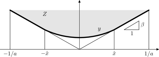
Figure 4.2: The $C^{1}$ competitor profile.

Minimum problem (4.18) corresponds to problem (4.15) under the assumption that the minimizer $Z$ is symmetric w.r.t. the $y$ axis, under mild integrability assumptions. By assuming that the optimal profile in (4.18) is actually not in contact with the constraint $\beta|x|$ in some (still unknown) interval $(-\hat{x},\hat{x})$ for some $\hat{x}\in(0,1/a)$, one can consider variations of ${\mathcal{F}}$ which are symmetric and compactly supported in $(-\hat{x},\hat{x})$ in order to compute the Euler-Lagrange equation

$$\frac{\mathrm{d}}{\mathrm{d}x}\frac{y^{\prime}(x)}{\sqrt{1+(y^{\prime}(x))^{2}}}=a.$$

We can now solve for $y^{\prime},$ taking into account $y^{\prime}(0+)=0$, and deduce that

$$y^{\prime}(x)=\frac{ax}{\sqrt{1-a^{2}x^{2}}}\quad\text{for all }x\in[0,\hat{x})$$

which, by direct integration gives

$$y(x)=y(0)-\frac{1}{a}\sqrt{1-a^{2}x^{2}}.$$

This in particular entails that, independently of the opening $\beta$, in case of no contact with the constraint $\beta|x|$ the optimal profile is an arc of a circle with radius $1/a$. Note indeed that the latter expression makes sense for $|x|\leq|\hat{x}|\leq 1/a$ only.

In order to determine $y(0)$, we ask $\hat{x}$ to be a tangency point between the optimal profile $y(x)$ and the constraint $\beta|x|$. Indeed, such tangency must occur at some point in $(0,1/a)$. If this were not the case, one could translate the profile as $y(x)-k$ for $k>0$ up to tangency, which would contradict minimality. We can hence assume that $y(\hat{x})=\beta\hat{x}$ and $y^{\prime}(\hat{x})=\beta$ (otherwise this very argument could be repeated at $\hat{x}$, giving rise to a contradiction). Moreover, $y(x)=\beta x$ for all $x\in(\hat{x},1/a)$, for the only other options would be to have an arc of radius $a$ in $(\hat{x},1/a)$ as well, which would again contradict minimality. This gives

$$\hat{x}=\frac{\beta}{a\sqrt{1+\beta^{2}}}\ \ \text{and}\ \ y(0)=\frac{1}{a}\sqrt{1+\beta^{2}}.$$

Note that $\hat{x}<1/a$ for all $\beta>0.$ In particular, the candidate optimal profile is

$$y(x)=-\frac{1}{a}\sqrt{1-a^{2}x^{2}}+\frac{1}{a}\sqrt{1+\beta^{2}}.$$ (4.19)

We now check that the $\mathrm{C}^{1}$ profile $y$ is optimal by comparing the value of ${\mathcal{F}}$ for $y$ with its value for the affine function $\ell(x)=\beta x;$ the latter corresponds to a nonreentrant corner (i.e., a point $x$ at the boundary such that the complement of the set locally contains a cone of amplitude strictly larger than $\pi$ and vertex at $x$). Using that $y\equiv\ell$ on $(\hat{x},1/a)$ we have

$${\mathcal{F}}(y)-{\mathcal{F}}(\ell) =\int_{0}^{\hat{x}}\sqrt{1+\frac{a^{2}x^{2}}{1-a^{2}x^{2}}}\,{\rm d}x-\sqrt{1+\beta^{2}}\hat{x}+a\int_{0}^{\hat{x}}\left(-\frac{1}{a}\sqrt{1-a^{2}x^{2}}+\frac{1}{a}\sqrt{1+\beta^{2}}-\beta x\right)\,{\rm d}x$$

$$=\int_{0}^{\hat{x}}\frac{a^{2}x^{2}}{\sqrt{1-a^{2}x^{2}}}\,{\rm d}x-\frac{\beta^{3}}{2a(1+\beta^{2})}<\frac{\beta^{3}}{3a(1+\beta^{2})^{3/2}}-\frac{\beta^{3}}{2a(1+\beta^{2})}<0.$$

This in particular shows that a nonreentrant corner at scale $1/a$ is not admissible and that the minimizer is $\mathrm{C}^{1}$ instead. On the other hand, the above argument is scale-invariant and nonreentrant corners are hence excluded at any scale. Note that the optimal profile $y$ is not $\mathrm{C}^{2}$, since $y^{\prime\prime}(\hat{x}-)>0$.

By combining this analysis with the remark on preservation of convexity, we can conclude that, in case $F^{c}$ is convex and piecewise $\mathrm{C}^{1}$, the minimizer of problem (4.15) is globally $\mathrm{C}^{1}$, see also Figures 4.7 (left and right) and 4.8 (left). This remark makes the conclusions of Proposition 4.3 sharper, for in two space dimensions one can choose $\mathfrak{a}=1/2$.

Regular polygonal forcing.

In view of the above discussion, the minimizer $Z$ of (4.15) can be explicitly determined in case $F^{c}$ is a regular polygon and $1/a$ is smaller than half its side. Indeed, the preservation of symmetries implies that the minimizer $Z$ shares the same symmetries of $F^{c}$, with rounded corners of radius $1/a$, see Figure 4.3.

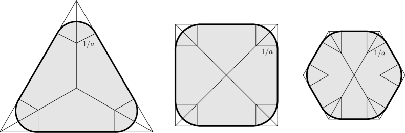
Figure 4.3: Solutions of the minimization problem (4.15) with forcing $F^{c}$ being an equilateral triangle, a square, and a regular hexagon, respectively.

Examples 4.8 (Nontrivial evolutions under compatibility condition (4.11)).

Let $B_{r}$ denote the open ball in $\mathbb{R}^{d}$ with radius $r\geq 0$. By imposing the compatibility condition (4.11) one has that

$$P(B_{r},\Omega)=a{\mathcal{L}}(B_{r})\quad\Leftrightarrow\quad\omega_{d}r^{d-1}=a\frac{\omega_{d}}{d}r^{d}$$

where $\omega_{d}$ is the surface of the unit sphere in $\mathbb{R}^{d}$. Hence, the only ball fulfilling (4.11) has radius $d/a$. An evolution under condition (4.11) and spherical symmetry is necessarily trivial: the ball of radius $d/a$ vanishes as soon as it is forced to evolve. Still, a first nontrivial evolution example can be obtained by considering a disjoint collection of balls of radius $d/a$. For instance, the two-dimensional set

$$Z(t)=\displaystyle\cup_{i=1}^{m(t)}B((i,0),2/a)\quad\text{for}\ \ m(t)=M-\lfloor t\rfloor$$ (4.20)

for some $M\in{\mathbb{N}}$ (and $2/a<1/2$) (with $\lfloor\cdot\rfloor$ the Gauss-bracket), gives an evolution corresponding to the forcing $F^{c}(t)=Z(t)$ and fulfills (4.11) for all times, see Figure 4.4.

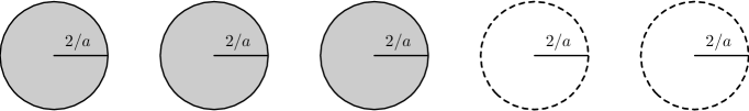
Figure 4.4: The evolution from (4.20) for $M=5$ and time $t=2$.

In two dimensions, condition (4.11) selects the unique minimizer among each family of rounded polygonal shapes, see Figure 4.3. By considering a collection of disjoint smoothed polygons fulfilling condition (4.11) and balls of radius $2/a$ (hence fulfilling condition (4.11)), one can again design a nontrivial evolution in the spirit of Figure 4.4.

Let us conclude by showing an example of a nontrivial evolution for a connected $Z(t)$ in two dimensions. Consider the smoothed square in the middle of Figure 4.3. Elementary algebra shows that the only smoothed square fulfilling condition (4.11) is inscribed in the square of side $(2+\sqrt{\pi})/a$. In particular, the flat portion of each side measures $\sqrt{\pi}/a\sim 1.77/a$. Let us now consider the union of discs of radius $1/a$ and the smoothed square, as in Figure 4.5. This union can be realized by still fulfilling condition (4.11), as long as the positioning of each extra disc is such that the gain in perimeter equates $a$-times the gain in area. By calling $\alpha$ the angle at the center of the disk which identifies the arc cut by the side of the smoothed square, the aforementioned equality reduces to

$$2\pi-\alpha-4\sin(\alpha/2)-\sin(\alpha)=0$$

(note that it is independent of $a$), whose unique solution in $[0,\pi]$ is $\tilde{\alpha}\sim 2.005$. Note that the cord of the disk of radius $1/a$ corresponding to $\tilde{\alpha}$ has length $2\sin(\tilde{\alpha}/2)/a\sim 1.687/a$, which is strictly shorter than the flat portion of each side of the smoothed square.

Figure 4.5: An evolution of connected sets fulfilling the compatibility condition (4.11), time flows from left to right.

All configurations in Figure 4.5 hence fulfill condition (4.11). Moreover, they are stable (with respect to the forcing corresponding to the interior of their complement), for they fulfill the interior ball condition with balls of radius $1/a$. An evolution as depicted in Figure (4.5) (left to right) can hence be realized by suitably prescribing the forcing. At all times, such evolution fulfills (4.11).

.

4.2 A numerical test

In order to illustrate the above discussion, we provide some numerical evidence in a planar setting. We assume $\Omega=(-3,3)^{2}$ and consider an initial state $Z^{o}\subset\Omega$ such that $F^{c}\subset Z^{o}$ where

$$F=\{(x,y)\in[0,1]\times[-1,1]\ :\ |y|>v(x)\}\cup\{(x,y)\in\mathbb{R}^{2}\ :\ x<0\ \text{or}\ x>1\},$$

where $v:[0,1]\to(0,1]$ is a given function, different for each numerical example. In the following, we seek minimizers $Z$ of the incremental problem (4.15) of the form

$$Z=\{(x,y)\in[0,1]\times[-1,1]\ :\ |y|\leq u(x)\}$$

for some optimal profile $u:[0,1]\to[0,1]$ to be determined such that $u(x)\leq v(x)$ for all $x\in[-1,1]$, which is in accordance with the brittle constraint $Z\subset F^{c}$. Note that, given the discussion on symmetry from Subsection 4.1, assuming $Z$ to be symmetric with respect to $\{y=0\}$ is not restrictive, since $F^{c}$ also is. Moreover, owing to the discussion leading to (4.19), it is not restrictive to assume that $[0,1]\times\{0\}\subset Z$ (that is, $Z$ can actually be described by the profile $u$) as long as the optimal profile $u$ fulfills

$$u(x)\geq\sqrt{(a^{2}-(x{-}a)^{2})^{+}}+\sqrt{(a^{2}-(x{-}1{+}a)^{2})^{+}}\quad\forall x\in[0,1]$$

(that is, if $Z$ contains the two balls of radius $a$ centered in $(a,0)$ and $(1{-}a,0)$), which happens to be the case for all computations below.

The problem is discretized in space by partitioning the domain $[0,1]$ of the variable $x$ as $0=x_{0}<x_{1}<\dots<x_{N}=1$ with $x_{i}=i/N$ and $N=100$ and by approximating $v$ via its piecewise affine interpolant on the partition, taking the values $v(i/N)=:v_{i}$. In particular, we look for $u$ piecewise affine with $u(i/N)=:u_{i}$ minimizing

$$(u_{0},\dots,u_{N}) \mapsto P(Z,\Omega)+a{\mathcal{L}}^{2}(F^{c}{\setminus}Z)$$

$$=2\left(u_{0}+u_{N}+\sum_{i=1}^{N}\sqrt{(u_{i}{-}u_{i-1})^{2}+N^{-2}}+a\sum_{i=1}^{N}N^{-1}|u_{i}-v_{i}|\right)$$

under the constraints $$0\leq u_{i}\leq v_{i} i=1,\dots,N$$ for .

This is a strictly convex minimization problem under convex constraints. In the following, we solve it by using the fmincon tool of Matlab for different choices of the function $v$. In all figures, we depict the portions of the minimizer $Z$ (light color) and of the forcing set $F$ in $[0,1]^{2}$ (dark color). The reader should however keep in mind that both forcing and minimizer are actually symmetric along $\{y=0\}$.

Figure 4.6 corresponds to the choice $v(x)=(x{-}1/2)^{2}+1/2$ and illustrates the effect of changing the parameter $a$. A smaller value of $a$ favors a shorter perimeter at the expense of a larger distance from $F^{c}$. Correspondingly, the top adhesion zone, namely the points where $u\equiv v$, is smaller for smaller $a$.

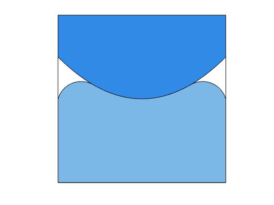
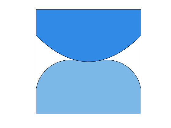
Figure 4.6: The effect of changing the parameter $a$. The two solutions correspond to $v(x)=(x{-}1/2)^{2}+1/2$ for $a=7$ (left) and $a=3$ (right). The top adhesion zone is smaller for smaller $a$. Note that the parts of the boundary of $Z$ which are not in contact with $F^{c}$ are arcs of circles with radius $1/a$ (recall that $a$ is different in the two figures), as predicted in Subsection 4.1.

Let us mention that, in case $a<2$ one can prove that $u_{0}=u_{N}=0$ which, as mentioned above, may well be not admissible. In order to avoid this pathology, in all the following simulations, the parameter $a$ will be always chosen to be $5$. Correspondingly, in all simulations the optimal profile $u$ is everywhere well separated from the $y=0$ axis.

Figure 4.7 follows by letting $v(x)=3/4-\beta(x{-}1/2)^{2}$ along with two different choices of the parameter $\beta$ and is meant to illustrate the convexity of the evolution in presence of a convex forcing $F^{c}$, see Subsection 4.1. In particular, the minimizer $Z$ is convex. One observes that the optimal profile $u$ detaches from $v$ even in the convex case. This is indeed the case also in Figure 4.7 left, where nonetheless the detachement is not visible due to the scale.

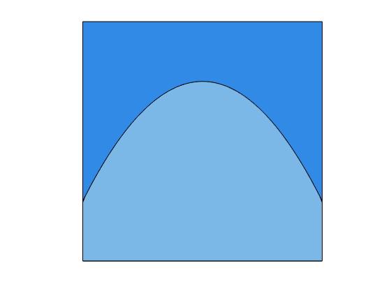
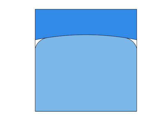
Figure 4.7: Convex forcing $F^{c}$. The two solutions correspond to $v(x)=3/4-\beta(x{-}1/2)^{2}$ for $\beta=2$ (left) and $\beta=1/5$ (right). The minimal set $Z$ is convex.

Figure 4.8 corresponds to the choices $v(x)=1/2\pm(|x{-}1/2|-1/4)$ and illustrates the partial regularity of the solution. Note that nonsmooth boundary points occur in connection with nonconvex forcings $F^{c}$.

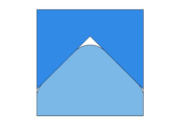
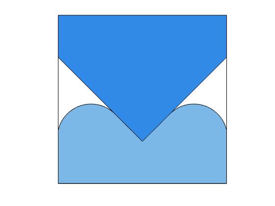
Figure 4.8: Partial $C^{1}$ regularity. The two solutions correspond to $v(x)=3/4-|x{-}1/2|$ (left) and $v(x)=1/4+|x{-}1/2|$ (right).

Figure 4.9 illustrates some special situations. On the left, the solution for $v(x)=\max\{1-5|x{-}1/2|,1/2\}$. In this case, the optimal profile is such that $u(1/2)>3/4$. Note that the same holds for any opening of the cone in $F^{c}$, whatever small. On the right, the solution for $v(x)=\lfloor 5x\rfloor/5+1/5$. The profiles $u=v$ touch at the points $x=1/5,\,2/5,\,3/5$, and $4/5$ only. Note that all nonstraight portions of the boundary of $Z$ are arcs of radius $1/a$.

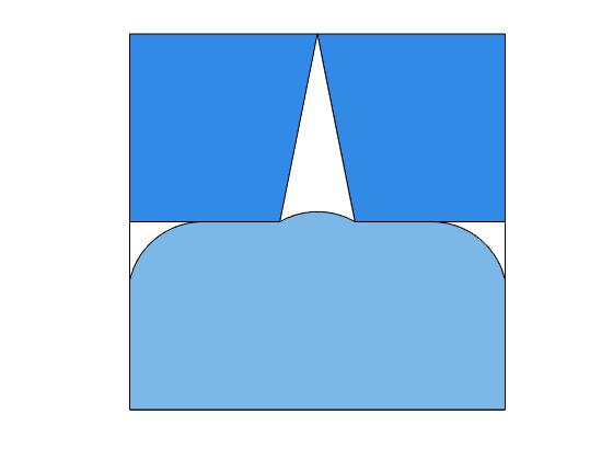
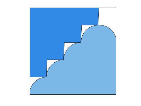
Figure 4.9: Extreme configurations. The solution for $v(x)=\max\{1-5|x{-}1/2|,1/2\}$ (left) and $v(x)=\lfloor 5x\rfloor/5+1/5$ (right).

5 Proofs of Theorems 4.1, 4.5, and 4.6

We start by the Proof of Theorem 4.1: For $k\in\mathbb{N}\cup\{\infty\}$ fixed, let $(\tau_{j})_{j}$ be a vanishing sequence and let $(\overline{z}_{\kern-1.0pt\tau_{j}})_{j}$ be the characteristic functions of the sets $(\overline{Z}_{\kern-1.0pt\tau_{j}})_{j}$. Since the functions $\overline{z}_{\kern-1.0pt\tau_{j}}$ are nonincreasing, it is immediate to check that

$$\exists\,C>0\ \forall\,j\in\mathbb{N}\,:\qquad\|\overline{z}_{\kern-1.0pt\tau_{j}}\|_{\mathrm{BV}([0,T];L^{1}(\Omega))}\leq C\,.$$

Furthermore, from (3.8) we get that

$$\exists\,C>0\ \forall\,j\in\mathbb{N}\,:\qquad\|\overline{z}_{\kern-1.0pt\tau_{j}}\|_{L^{\infty}(0,T;\mathrm{SBV}(\Omega;\{0,1\}))}\leq C\,.$$

We are now in the position to apply a Helly-type compactness result (cf. e.g. [MM05, Thm. 3.2]), and conclude that

$$\exists\,z\in L^{\infty}(0,T;\mathrm{SBV}(\Omega;\{0,1\}))\cap\mathrm{BV}([0,T];L^{1}(\Omega)),$$

$$\quad\text{with }z(\cdot,x)\text{ nonincreasing on }[0,T]\ \text{for a.a.}\,x\in\Omega,\text{ such that }$$

$$\overline{z}_{\kern-1.0pt\tau_{j}}(t)\overset{*}{\rightharpoonup}z(t)\quad\text{ in }\mathrm{SBV}(\Omega;\{0,1\})\quad\text{for every }t\in[0,T].$$

Then, the curve $Z:[0,T]\to\mathbf{X}$ defined by $Z(0)=Z_{0}$ and $Z(t):=\{x\in\Omega\,:\ z(t)=1\}$ for all $t\in(0,T]$ is in $\mathrm{GMM}(\mathbf{Z},{\mathcal{E}}_{k},{\mathcal{D}};Z_{0})$.

In order to prove convergence (4.1a) for the piecewise constant, right-continuous interpolants $(\underline{z}_{\kern-1.0pt\tau_{j}})_{j}$ we may argue in this way: by the above Helly argument, there exists $\underline{z}\in L^{\infty}(0,T;\mathrm{SBV}(\Omega;\{0,1\}))\cap\mathrm{BV}([0,T];L^{1}(\Omega))$ such that, up to a further subsequence, $\underline{z}_{\kern-1.0pt\tau_{j}}(t)\overset{*}{\rightharpoonup}\underline{z}(t)$ in $\mathrm{SBV}(\Omega;\{0,1\})$ for all $t\in[0,T]$. Let $J$ be the union of the jump sets of $z$ and $\underline{z}$: arguing for instance as in the proof of [RTP15, Thm. 4.1], it can be checked that $z(t)=\underline{z}(t)$ for all $t\in[0,T]\setminus J$. Convergences (4.1b) and (4.1c) ensue from standard weak and strong compactness arguments.

Let us now pick $Z\in\mathrm{GMM}(\mathbf{Z},{\mathcal{E}}_{k},{\mathcal{D}};Z_{0})$ approximated by a sequence $(\overline{Z}_{\kern-1.0pt\tau_{j}})_{j}$ in the sense of (2.21). In order to show that $Z$ satisfies the stability condition (2.22), we will pass to the limit in its discrete version (3.7), satisfied by the functions $\overline{Z}_{\kern-1.0pt\tau_{j}}$, by verifying the so-called mutual recovery sequence condition from [MRS08]. Namely, for every fixed $t\in(0,T]$ and every admissible competitor $\widetilde{Z}\in\mathbf{X}$ for (2.22), with associated characteristic function $\tilde{z}$, we will exhibit a sequence $(\tilde{z}_{j})_{j}\subset\mathrm{SBV}(\Omega;\{0,1\})$ such that

$$\limsup_{j\to\infty}\left({\mathcal{E}}_{k}(t,\tilde{z}_{j}){-}{\mathcal{E}}_{k}(t,\overline{z}_{\kern-1.0pt\tau_{j}}(t)){+}{\mathcal{D}}(\overline{z}_{\kern-1.0pt\tau_{j}}(t),\tilde{z}_{j})\right)\leq{\mathcal{E}}_{k}(t,\tilde{z}){-}{\mathcal{E}}_{k}(t,z(t)){+}{\mathcal{D}}(z(t),\tilde{z})\,.$$ (5.1)

The construction of the sequence $(\tilde{z}_{j})_{j}$ is slightly adapted from the proof of [RT15, Prop. 5.9], which in turn follows the steps of [Tho13, Lemma 2.13]. Hence, in the following lines we shall refer to [RT15] for some details. First of all, we suppose that ${\mathcal{D}}(z(t),\tilde{z})<\infty$, whence $\tilde{z}\leq z(t)$ a.e. in $\Omega$, and, if $k=\infty$, that ${\mathcal{J}}_{\infty}(t,\tilde{z})=0$, so that ${\mathcal{E}}_{\infty}(t,\tilde{z})<\infty$; otherwise, there is nothing to prove. Along the foosteps of [RT15], we set

$$\tilde{z}_{j}:=\tilde{z}\chi_{A_{j}}+\overline{z}_{\kern-1.0pt\tau_{j}}(t)(1{-}\chi_{A_{j}}),\quad\text{where }A_{j}:=\{x\in\Omega\,:\ 0\leq\tilde{z}(x)\leq\overline{z}_{\kern-1.0pt\tau_{j}}(t,x)\}\,.$$ (5.2)

This way, we ensure that

$$\tilde{z}_{j}\in\{0,1\}\quad\text{and}\quad 0\leq\tilde{z}_{j}\leq\overline{z}_{\kern-1.0pt\tau_{j}}(t)\qquad\text{a.e. in}\ \Omega\,.$$ (5.3)

Furthermore, arguing in the very same way as in the proof of [RT15, Prop. 5.9], where [AFP05, Thm. 3.84] on the decomposition of $\mathrm{BV}$-functions is applied, we can show that $\tilde{z}_{j}\in\mathrm{SBV}(\Omega;\{0,1\})$. We now split the proof of (5.1) in $3$ steps:

1. Since

   $$\overline{z}_{\kern-1.0pt\tau_{j}}(t)\to z(t)\qquad\text{in $L^{q}(\Omega)$ for all $1\leq q<\infty$},$$ (5.4)

   and $\tilde{z}\leq z(t)$ a.e. in $\Omega$, it is immediate to infer that $\tilde{z}_{j}\to\tilde{z}$ a.e. in $\Omega$ as $j\to\infty$, which improves to

   $$\tilde{z}_{j}\to\tilde{z}\quad\text{in }L^{q}(\Omega)\quad\text{for all }1\leq q<\infty,$$ (5.5)

   as $\tilde{z}_{j}\in\{0,1\}$ a.e. in $\Omega$. Combining (5.3) with (5.4) and (5.5) we ultimately conclude that

   $$\lim_{j\to\infty}{\mathcal{D}}(\overline{z}_{\kern-1.0pt\tau_{j}}(t),\tilde{z}_{j})={\mathcal{D}}(z(t),\tilde{z})\,.$$ (5.6)

2. For $k\in\mathbb{N}$, we observe that

   $$\limsup_{j\to\infty}\left({\mathcal{J}}_{k}(t,\tilde{z}_{j}){-}{\mathcal{J}}_{k}(t,\overline{z}_{\kern-1.0pt\tau_{j}}(t))\right)=\limsup_{j\to\infty}\int_{\Omega}kf(t)(\tilde{z}_{j}{-}\overline{z}_{\kern-1.0pt\tau_{j}}(t))\,\mathrm{d}x =\int_{\Omega}kf(t)(\tilde{z}{-}z(t))\,\mathrm{d}x$$ (5.7a)

   $$={\mathcal{J}}_{k}(t,\tilde{z}){-}{\mathcal{J}}_{k}(t,z(t))$$

   thanks to (5.4) and (5.5). For $$k=\infty \sup_{j\in\mathbb{N}}{\mathcal{E}}(t,\overline{z}_{\kern-1.0pt\tau_{j}}(t))\leq C {\mathcal{J}}_{\infty}(t,\overline{z}_{\kern-1.0pt\tau_{j}}(t))=0 f(t,\cdot)\overline{z}_{\kern-1.0pt\tau_{j}}(t,\cdot)=0 \Omega j\in\mathbb{N} 0\leq{\mathcal{J}}_{\infty}(t,z(t))\leq\liminf_{j\to\infty}{\mathcal{J}}_{\infty}(t,\overline{z}_{\kern-1.0pt\tau_{j}}(t))=0 \tilde{z}_{j}\leq\overline{z}_{\kern-1.0pt\tau_{j}}(t) \Omega {\mathcal{J}}_{\infty}(t,\tilde{z}_{j})=0 j\in\mathbb{N}$$, we first of all observe that, since by (2.21), we have , i.e.  a.e. in , for every . Then, . Furthermore, since a.e. in thanks to (5.3), we ultimately conclude that for all . Therefore,

   $$\limsup_{j\to\infty}\left({\mathcal{J}}_{\infty}(t,\tilde{z}_{j}){-}{\mathcal{J}}_{\infty}(t,\overline{z}_{\kern-1.0pt\tau_{j}}(t))\right)=0={\mathcal{J}}_{\infty}(t,\tilde{z})-{\mathcal{J}}_{\infty}(t,z(t))$$ (5.7b)

   (recall that we have supposed right from the start that ${\mathcal{J}}_{\infty}(t,\tilde{z})=0$).

3. Finally, it can be shown that

   $$\limsup_{j\to\infty}\left(|\mathrm{D}\tilde{z}_{j}|(\Omega){-}|\mathrm{D}\overline{z}_{\kern-1.0pt\tau_{j}}(t)|(\Omega)\right)\leq|\mathrm{D}\tilde{z}|(\Omega){-}|\mathrm{D}z(t)|(\Omega)$$ (5.8)

   by repeating the very same arguments as in the proof of [RT15, Prop. 5.9].

Combining (5.6), (5.7), and (5.8), we infer (5.1) for $k\in\mathbb{N}$ and $k=\infty$, which concludes the proof of the stability condition (2.22), and thus of Thm. 4.1.  

Proof of Theorem 4.5:

Let $k\in\mathbb{N}$ be fixed, let $Z\in\mathrm{SMM}(\mathbf{Z},{\mathcal{E}}_{k},{\mathcal{D}};Z_{0})$, and let $(\overline{z}_{\kern-1.0pt\tau_{j}})_{j}$ converge to $z=\chi_{Z}$ as in (2.21). We can pass to the limit in the upper energy-dissipation estimate in (3.10) by observing that

$$\liminf_{j\to\infty}\left({\mathcal{E}}_{k}(\overline{\mathsf{t}}_{\kern-1.0pt\tau_{j}}(t),\overline{Z}_{\kern-1.0pt\tau_{j}}(t)){-}{\mathcal{E}}_{k}(t,z(t))\right)$$

$$\geq\lim_{j\to\infty}\left({\mathcal{E}}_{k}(\overline{\mathsf{t}}_{\kern-1.0pt\tau_{j}}(t),\overline{Z}_{\kern-1.0pt\tau_{j}}(t)){-}{\mathcal{E}}_{k}(t,\overline{Z}_{\kern-1.0pt\tau_{j}}(t))\right)+\liminf_{j\to\infty}\left({\mathcal{E}}_{k}(t,\overline{Z}_{\kern-1.0pt\tau_{j}}(t)){-}{\mathcal{E}}_{k}(t,z(t))\right)=:l_{1}+l_{2}\geq 0,$$

where we have used that

$$l_{1}=\lim_{j\to\infty}\int_{\Omega}k\left(f(\overline{\mathsf{t}}_{\kern-1.0pt\tau_{j}}(t),x){-}f(t,x)\right)\overline{z}_{\kern-1.0pt\tau_{j}}(t,x))\,\mathrm{d}x\leq k\lim_{j\to\infty}\int_{t}^{\overline{\mathsf{t}}_{\kern-1.0pt\tau_{j}}(t)}\|\partial_{t}f(s)\|_{L^{1}(\Omega)}\,\mathrm{d}s=0,$$

due to (2.1c), while, by convergence (2.21) we have

$$l_{2}=\liminf_{j\to\infty}\left(|\mathrm{D}\overline{z}_{\kern-1.0pt\tau_{j}}(t)|(\Omega){-}|\mathrm{D}z(t)|(\Omega)\right)\geq 0\,.$$

Thanks to (2.21), we also have $\liminf_{j\to\infty}{\mathcal{D}}(Z_{0},\overline{Z}_{\kern-1.0pt\tau_{j}}(t))\geq{\mathcal{D}}(Z_{0},Z(t))$, and (4.1) gives

$$\lim_{j\to\infty}\int_{0}^{\overline{\mathsf{t}}_{\kern-1.0pt\tau_{j}}(t)}\partial_{t}{\mathcal{E}}_{k}(r,\underline{Z}_{\kern-1.0pt\tau_{j}}(r))\,\mathrm{d}r =\lim_{j\to\infty}\int_{0}^{\overline{\mathsf{t}}_{\kern-1.0pt\tau_{j}}(t)}\int_{\Omega}k\partial_{t}f(r,x)\underline{z}_{\kern-1.0pt\tau_{j}}(r,x)\,\mathrm{d}x\,\mathrm{d}r$$

$$=\int_{0}^{t}\int_{\Omega}k\partial_{t}f(r,x)z(r,x)\,\mathrm{d}x\,\mathrm{d}r=\int_{0}^{t}\partial_{t}{\mathcal{E}}_{k}(r,Z(r))\,\mathrm{d}r\,.$$

All in all, we conclude the upper energy-dissipation estimate

$${\mathcal{E}}_{k}(t,Z(t))+{\mathcal{D}}(Z(0),Z(t))\leq{\mathcal{E}}_{k}(0,Z(0))+\int_{0}^{t}\partial_{t}{\mathcal{E}}_{k}(r,Z(r))\,\mathrm{d}r\qquad\text{for all }t\in[0,T].$$

The lower estimate $\geq$ follows from the stability condition (2.22) via a well-established Riemann-sum technique, cf. e.g. [MR15, Prop. 2.1.23] for a general result. This concludes the proof that $Z$ is an Energetic solution to the adhesive rate-independent system $(\mathbf{Z},{\mathcal{E}}_{k},{\mathcal{D}})$.  

Prior to proving Thm. 4.6, we show in the following result that, for every fixed $t\in[0,T]$, the energies ${\mathcal{E}}_{k}(t,\cdot)$ for the adhesive systems $\Gamma$-converge as $k\to\infty$ to the energy ${\mathcal{E}}_{\infty}(t,\cdot)$ driving the brittle system with respect to the weak^∗-topology of $\mathrm{SBV}(\Omega;\{0,1\})$ (in the sense of (2.5)). Namely, we shall prove that

$$\Gamma \liminf z_{k}\overset{*}{\rightharpoonup}z\text{ in }\mathrm{SBV}(\Omega;\{0,1\})\ \Rightarrow\ \liminf_{k\to\infty}{\mathcal{E}}_{k}(t,z_{k})\geq{\mathcal{E}}_{\infty}(t,z),$$- estimate: (5.9a)

$$\Gamma \limsup \forall\,\hat{z}\in\mathrm{SBV}(\Omega;\{0,1\})\ \exists\,(\hat{z}_{k})_{k}\subset\mathrm{SBV}(\Omega;\{0,1\})\,:\ \hat{z}_{k}\overset{*}{\rightharpoonup}\hat{z}\text{ in }\mathrm{SBV}(\Omega;\{0,1\})$$- estimate: (5.9b)

$$\qquad\qquad\text{ and }\limsup_{k\to\infty}{\mathcal{E}}_{k}(t,\hat{z}_{k})\leq{\mathcal{E}}_{\infty}(t,\hat{z})\,.$$

Lemma 5.1.

For every $t\in[0,T]$ the functionals $({\mathcal{E}}_{k}(t,\cdot)_{k}$ defined by (2.14) $\Gamma$-converge as $k\to\infty$, in the sense of (5.9), to ${\mathcal{E}}_{\infty}(t,\cdot)$ from (2.16).

Proof. To start with, observe that the upper estimate (5.9b) can be concluded by choosing the constant sequence $(\hat{z}_{k}:=\hat{z})_{k}$ as a recovery sequence.

To verify the lower estimate (5.9a), consider a sequence $z_{k}\overset{*}{\rightharpoonup}z$ in $\mathrm{SBV}(\Omega;\{0,1\})$ and the corresponding sets of finite perimeter $Z_{k},Z$. We distinguish two cases:

1. If ${\mathcal{L}}^{d}(Z\cap F(t))=0,$ then, by the positivity of ${\mathcal{J}}_{k}(t,\widetilde{Z}_{k})$ and the lower semicontinuity of the perimeter w.r.t. strong $L^{1}$-convergence of characteristic functions, we find that

   $$\liminf_{k\to\infty}{\mathcal{E}}_{k}(t,z_{k})\geq P(Z,\Omega)={\mathcal{E}}_{\infty}(t,z).$$

2. Assume now that ${\mathcal{L}}^{d}(Z\cap F(t))=c>0$, so that ${\mathcal{J}}_{\infty}(t,z)=\infty$. Since $z_{k}\to z$ strongly in $L^{1}(\Omega),$ we also have $f(t)z_{k}\to f(t)z$ strongly in $L^{1}(\Omega),$ and hence, for every $\varepsilon>0$ we find an index $k_{\varepsilon}\in\mathbb{N}$ such that for all $k\geq k_{\varepsilon}$ we have that $\|f(t)z_{k}-f(t)z\|_{L^{1}(\Omega)}\leq\varepsilon$. This implies that, for every $\varepsilon\in(0,c)$ there holds

   $$\liminf_{k\to\infty}{\mathcal{J}}_{k}(t,z_{k})=\liminf_{k\to\infty}\int_{\Omega}kf(t)z_{k}\,\mathrm{d}x\geq\liminf_{k\to\infty}k(c-\varepsilon)=\infty,$$

   whence again (5.9a).

 

We are now in a position to carry out the proof of Theorem 4.6: Let us consider a sequence $(Z_{k})_{k}$ with $Z_{k}\in\mathrm{SMM}(\mathbf{Z},{\mathcal{E}}_{k},{\mathcal{D}};Z_{0})$ for every $k\in\mathbb{N}$ and the associated sequence of characteristic functions $(z_{k})_{k}$. Since the energy bound (3.8) holds for a constant uniform w.r.t. $k\in\mathbb{N}$ as well, and it is inherited by the time-continuous limit, we infer

$$\exists\,C>0\ \forall\,k\in\mathbb{N}\,:\quad\sup_{t\in[0,T]}{\mathcal{E}}_{k}(t,z_{k}(t))\leq C,\ \text{ as well as }\ \mathrm{Var}_{{\mathcal{D}}}(z_{k};[0,T])\leq C$$

as the sequence $(z_{k})_{k}$ is nonincreasing in time. Hence we may repeat the very same compactness arguments as in the proof of Thm. 4.1 and conclude that there exist a (not relabeled) subsequence and $z\in L^{\infty}(0,T;\mathrm{SBV}(\Omega;\{0,1\}))\cap\mathrm{BV}([0,T];L^{1}(\Omega))$ such that (2.5) holds, as well as

$$z_{k}\overset{*}{\rightharpoonup}z\text{ in }L^{\infty}(0,T;\mathrm{SBV}(\Omega;\{0,1\})),\qquad z_{k}\to z\text{ in }L^{q}((0,T){\times}\Omega)\text{ for every }q\in[1,\infty).$$ (5.10)

Thanks to Lemma 5.1 we have

$$\liminf_{k\to\infty}{\mathcal{E}}_{k}(t,z_{k}(t))\geq{\mathcal{E}}_{\infty}(t,z(t)),\quad\text{in particular }{\mathcal{J}}_{\infty}(t,z(t))=0,\quad\text{for all }t\in[0,T].$$ (5.11)

The limit passage as $k\to\infty$ in the stability condition (2.22), for $t\in(0,T]$ fixed, again relies on the mutual recovery sequence condition, i.e. on the fact that for every $\tilde{z}\in\mathrm{SBV}(\Omega;\{0,1\})$ (with ${\mathcal{D}}(z(t),\tilde{z})<\infty$ and ${\mathcal{J}}_{\infty}(t,\tilde{z})=0$ to avoid trivial situations) there exists $(\tilde{z}_{k})_{k}\subset\mathrm{SBV}(\Omega;\{0,1\})$ such that

$$\limsup_{k\to\infty}\left({\mathcal{E}}_{k}(t,\tilde{z}_{k}){-}{\mathcal{E}}_{k}(t,z_{k}(t)){+}{\mathcal{D}}(z_{k}(t),\tilde{z}_{k})\right)\leq{\mathcal{E}}_{\infty}(t,\tilde{z}){-}{\mathcal{E}}_{\infty}(t,z(t)){+}{\mathcal{D}}(z(t),\tilde{z})\,.$$ (5.12)

To this end, we resort to a construction completely analogous to that in (5.2) and set

$$\tilde{z}_{k}:=\tilde{z}\chi_{A_{k}}+z_{k}(t)(1{-}\chi_{A_{k}})\quad\text{with }A_{k}:=\{x\in\Omega\,:\ 0\leq\tilde{z}(x)\leq z_{k}(t,x)\}\,.$$ (5.13)

Exploiting the convergence properties (5.6), (5.8), as well as the fact that

$$\limsup_{k\to\infty}\left({\mathcal{J}}_{k}(t,\tilde{z}_{k})-{\mathcal{J}}_{k}(t,z_{k}(t))\right)=\limsup_{k\to\infty}\int_{\Omega}kf(t,x)\left(\tilde{z}_{k}(t,x){-}z_{k}(t,x)\right)\,\mathrm{d}x\leq 0={\mathcal{J}}_{\infty}(t,\tilde{z})-{\mathcal{J}}_{\infty}(t,z(t))$$

(since $\tilde{z}_{k}\leq z_{k}$ a.e. in $\Omega$ by construction), we obtain (5.12). This proves that $Z\in\mathrm{SMM}(\mathbf{Z},{\mathcal{E}}_{\infty},{\mathcal{D}};Z_{0})$.

In order to conclude that $Z$ is an Energetic solution to the brittle system $(\mathbf{Z},{\mathcal{E}}_{\infty},{\mathcal{D}})$ under the additional monotonicity assumption $\partial_{t}f\geq 0$ and compatibilty condition (4.11), we first establish the upper energy-dissipation estimate

$${\mathcal{E}}_{\infty}(t,z(t))+{\mathcal{D}}(z(0),z(t))\leq{\mathcal{E}}_{\infty}(0,Z_{0})\quad\text{for all }t\in[0,T]$$ (5.14)

by passing to the limit in (1.7) as $k\to\infty$. With this aim, we observe that

$${\mathcal{J}}_{k}(t,z_{k}(t))=\int_{\Omega}kf(t)z_{k}(t)\,\mathrm{d}x\to 0\quad\text{as }k\to\infty\quad\text{for all }t\in[0,T].$$ (5.15)

To check (5.15), first of all we apply the construction of the recovery sequence (5.13) to $\tilde{z}:=z(t)$ to find a sequence $(\tilde{z}_{k})_{k}$, associated with sets $(\widetilde{Z}_{k})_{k}$. As observed in the proof of Theorem 4.1 (cf. (5.8)), the construction ensures in particular that $\limsup_{k\to\infty}\big{(}|\mathrm{D}\tilde{z}_{k}|(\Omega){-}|\mathrm{D}z_{k}(t)|(\Omega)\big{)}\leq|\mathrm{D}z(t)|(\Omega)-|\mathrm{D}z(t)|(\Omega)=0$. Moreover, $\tilde{z}_{k}\leq\min\{z_{k}(t),\,z(t)\}$ a.e. in $\Omega$ and $\tilde{z}_{k}\to z(t)$ in $L^{1}(\Omega)$, so that

$$\lim_{k\to\infty}{\mathcal{D}}(z_{k}(t),\tilde{z}_{k})=0.$$

Also observe that ${\mathcal{J}}_{k}(t,\tilde{z}_{k})=0$ for all $k\in\mathbb{N},$ because ${\mathcal{J}}_{\infty}(t,z(t))=0$ by (5.11) and because $\widetilde{Z}_{k}\subset Z(t)$ by construction. Since ${\mathcal{J}}_{k}(t,z_{k}(t))\geq 0$ for all $k\in\mathbb{N}$, these observations allow us to conclude from the stability of $z_{k}(t)$ that

$$0\leq\liminf_{k\to\infty}{\mathcal{J}}_{k}(t,z_{k}(t))\leq\limsup_{k\to\infty}{\mathcal{J}}_{k}(t,z_{k}(t))\leq\limsup_{k\to\infty}\big{(}P(\widetilde{Z}_{k},\Omega)-P(Z_{k}(t),\Omega)\big{)}+\lim_{k\to\infty}{\mathcal{D}}(z_{k}(t),\tilde{Z}_{k})=0\,,$$

which gives (5.15). We will now show that

$$\int_{0}^{t}\partial_{t}{\mathcal{E}}_{k}(s,z_{k}(s))\,\mathrm{d}s=\int_{0}^{t}\int_{\Omega}k\partial_{t}f(s)z_{k}(s)\,\mathrm{d}x\,\mathrm{d}s\to 0\quad\text{as }k\to\infty\quad\text{for all }t\in[0,T].$$ (5.16)

Indeed, using the assumption $\partial_{t}f\geq 0$ the energy balance (1.7) for each $k\in\mathbb{N}$ gives

$$0 \leq\int_{0}^{t}\int_{\Omega}k\partial_{t}f(s)z_{k}(s)\,\mathrm{d}x\,\mathrm{d}s$$ (5.17)

$$=P(Z_{k}(t),\Omega)+{\mathcal{J}}_{k}(t,z_{k}(t))+{\mathcal{D}}(Z_{0}^{k},Z_{k}(t))-P(Z_{0}^{k},\Omega)-{\mathcal{J}}_{k}(0,Z_{0}^{k})$$

$$\stackrel{{\scriptstyle(1)}}{{\leq}}{\mathcal{D}}(Z_{k}(t),\emptyset)+{\mathcal{D}}(Z_{0}^{k},Z_{k}(t))-P(Z_{0}^{k},\Omega)\stackrel{{\scriptstyle(2)}}{{=}}{\mathcal{D}}(Z_{0}^{k},\emptyset)-P(Z_{0}^{k},\Omega)\,,$$

where (1) follows from observing that ${\mathcal{J}}_{k}(0,Z_{0}^{k})\geq 0$ and from choosing $\widetilde{Z}=\emptyset$ in the stability condition (2.22) (which gives $P(Z_{k}(t),\Omega)+{\mathcal{J}}_{k}(t,z_{k}(t))\leq{\mathcal{D}}(Z_{k}(t),\emptyset)$), while (2) ensues from the fact that

$${\mathcal{D}}(Z_{k}(t),\emptyset)+{\mathcal{D}}(Z_{0}^{k},Z_{k}(t))=a{\mathcal{L}}^{d}(Z_{k}(t))+a{\mathcal{L}}^{d}(Z_{0}^{k}{\setminus}Z_{k}(t))=a{\mathcal{L}}^{d}(Z_{0}^{k})={\mathcal{D}}(Z_{0}^{k},\emptyset)\,.$$

We then observe that

$$\lim_{k\to\infty}\left({\mathcal{D}}(Z_{0}^{k},\emptyset){-}P(Z_{0}^{k},\Omega)\right)\stackrel{{\scriptstyle(3)}}{{=}}{\mathcal{D}}(Z_{0},\emptyset)-P(Z_{0},\Omega)\stackrel{{\scriptstyle(4)}}{{=}}0\qquad\text{as }k\to\infty\,,$$

where (3) is due to condition (4.13) and (4) follows from the compatibility condition (4.11). Hence we conclude (5.16). Thus, (5.14) follows from passing to the limit as $k\to\infty$ in the upper estimate ’$\leq$’ of (2.24): the left-hand side is dealt with by lower semicontinuity arguments, while the limit passage on the right-hand side follows from the well-preparedness (4.10) of the initial data, and from (5.16).

The lower energy-dissipation estimate, i.e. the converse of inequality (5.14), follows from testing the stability condition at $t=0$ with $\widetilde{Z}=Z(t)$, which gives

$${\mathcal{E}}_{\infty}(0,Z_{0})\leq{\mathcal{D}}(Z(0),Z(t))+{\mathcal{E}}_{\infty}(0,Z(t))\leq{\mathcal{D}}(Z(0),Z(t))+{\mathcal{E}}_{\infty}(t,Z(t)).$$

Indeed, ${\mathcal{E}}_{\infty}(0,Z(t))-{\mathcal{E}}_{\infty}(t,Z(t))={\mathcal{J}}_{\infty}(0,Z(t))-{\mathcal{J}}_{\infty}(t,Z(t))=0$, since $Z(t)\cap F(t)=\emptyset$ and $F(0)\subset F(t)$ imply $Z(t)\cap F(0)=\emptyset$.

We have thus shown that $Z$ complies with the stability condition (2.22) and with the energy-dissipation balance (2.24). This concludes the proof of Theorem 4.6.  

Remark 5.2.

Assume that the external loading $f$ for the adhesive system complies with (4.9), and that the initial datum $Z_{0}$ satisfies the compatibility condition (4.11). From (5.17) we then deduce that

$$0=\int_{0}^{t}\int_{\Omega}k\partial_{t}f(s)z_{k}(s)\,\mathrm{d}x\,\mathrm{d}s=\int_{0}^{t}\partial_{t}{\mathcal{E}}_{k}(s,z_{k}(s))\,\mathrm{d}s$$

for every $t\in(0,T]$ and for all $k\in\mathbb{N}$. Therefore, $\partial_{t}fz_{k}=0$ a.e. in $\Omega\times(0,T)$, i.e. the sets $Z_{k}$ fulfill

$$Z_{k}(t)\subset({\mathop{\mathrm{supp}}}(\partial_{t}f(t)))^{c}\qquad\text{for a.a.}\,t\in(0,T)\,.$$ (5.18)

Taking into account that $(\mathop{\mathrm{supp}}(f(t)))^{c}\subset(\mathop{\mathrm{supp}}(\partial_{t}f(t)))^{c}$, (5.18) may be interpreted as a weak form of the brittle constraint (1.1).

References

- [AFP05] L. Ambrosio, N. Fusco, and D. Pallara. Functions of bounded variation and free discontinuity problems. Oxford University Press, 2005.
- [AGS08] L. Ambrosio, N. Gigli, and G. Savaré. Gradient flows in metric spaces and in the space of probability measures. Lectures in Mathematics ETH Zürich. Birkhäuser Verlag, Basel, second edition, 2008.
- [Amb95] L. Ambrosio. Minimizing movements. Rend. Accad. Naz. Sci. XL Mem. Mat. Appl. (5), 19:191–246, 1995.
- [ATW93] F. Almgren, J. E. Taylor, and L. Wang. Curvature-driven flows: A variational approach. SIAM J. Control Optim., 31(2):387–438, March 1993.
- [BBL08] D. Bucur, G. Buttazzo, and A. Lux. Quasistatic evolution in debonding problems via capacitary methods. Arch. Ration. Mech. Anal., 190(2):281–306, 2008.
- [Cam63] S. Campanato. Proprietà di hölderianità di alcune classi di funzioni. Ann. Sc. Norm. Super. Pisa Cl. Sci. (3), 17:175–188, 1963.
- [Cam64] S. Campanato. Proprietà di una famiglia di spazi funzionali. Ann. Sc. Norm. Super. Pisa Cl. Sci. (3), 18:137–160, 1964.
- [DMT02] G. Dal Maso and R. Toader. A model for the quasi-static growth of brittle fractures: existence and approximation results. Arch. Ration. Mech. Anal., 162(2):101–135, 2002.
- [FF09] A. Ferriero and N. Fusco. A note on the convex hull of sets of finite perimeter in the plane. Discrete Contin. Dyn. Syst. Ser. B, 11(1):103–108, 2009.
- [FF95] I. Fonseca and G. A. Francfort. Relaxation in versus quasiconvexification in ; a model for the interaction between fracture and damage. Calc. Var. Partial Differential Equations, 3:407–446, 1995.
- [FM98] G. A. Francfort and J.-J. Marigo. Revisiting brittle fracture as an energy minimization problem. J. Mech. Phys. Solids, 46(8):1319–1342, 1998.
- [Fré88] M. Frémond. Contact with adhesion. In J.J. Moreau, P.D. Panagiotopoulos, and G. Strang, editors, Topics in Nonsmooth Mechanics, pages 157–186. Birkhäuser, 1988.
- [Fré02] M. Frémond. Non-smooth thermomechanics. Springer-Verlag, Berlin, 2002.
- [Kaw86] B. Kawohl. On starshaped rearrangement and applications. Trans. Amer. Math. Soc., 296(1):377–386, 1986.
- [KL09] P. Krejčí and M. Liero. Rate independent Kurzweil processes. Appl. Math., 54(2):117–145, 2009.
- [KMR06] M. Kočvara, A. Mielke, and T. Roubíček. A rate-independent approach to the delamination problem. Math. Mech. Solids, 11:423–447, 2006.
- [LS95] S. Luckhaus and T. Sturzenhecker. Implicit time discretization for the mean curvature flow equation. Calc. Var. Partial Differential Equations, 3(2):253–271, Mar 1995.
- [MM05] A. Mainik and A. Mielke. Existence results for energetic models for rate-independent systems. Calc. Var. Partial Differential Equations, 22:73–99, 2005.
- [MR15] A. Mielke and T. Roubíček. Rate-independent systems: theory and application, volume 193 of Applied Mathematical Sciences. Springer, New York, 2015.
- [MRS08] A. Mielke, T. Roubíček, and U. Stefanelli. -limits and relaxations for rate-independent evolutionary problems. Calc. Var. Partial Differ. Equations, 31:387–416, 2008.
- [MT99] A. Mielke and F. Theil. A mathematical model for rate-independent phase transformations with hysteresis. In H.-D. Alber, R.M. Balean, and R. Farwig, editors, Proceedings of the Workshop on “Models of Continuum Mechanics in Analysis and Engineering”, pages 117–129, Aachen, 1999. Shaker-Verlag.
- [MT04] A. Mielke and F. Theil. On rate–independent hysteresis models. NoDEA Nonlinear Differential Equations Appl. N, 11:151–189, 2004.
- [RSZ09] T. Roubíček, L. Scardia, and C. Zanini. Quasistatic delamination problem. Contin. Mech. Thermodyn., 21(3):223–235, 2009.
- [RT15] R. Rossi and M. Thomas. From an adhesive to a brittle delamination model in thermo-visco-elasticity. wias-preprint 1692. ESAIM Control Optim. Calc. Var., 21:1–59, 2015.
- [RTP15] T. Roubíček, M. Thomas, and C. G. Panagiotopoulos. Stress-driven local-solution approach to quasistatic brittle delamination. Nonlinear Anal. Real World Appl., 22:645–663, 2015.
- [Tho13] M. Thomas. Quasistatic damage evolution with spatial BV-regularization. Discrete Contin. Dyn. Syst. Ser. S, 6(1): 235–255, 2013.
- [Tho15] M. Thomas. Uniform Poincaré-Sobolev and isoperimetric inequalities for classes of domains. Discrete Contin. Dyn. Syst., 35(6):2741–2761, 2015.
- [Vis97] A. Visintin. Motion by mean curvature and nucleation. C. R. Acad. Sci. Paris Sér. I Math., 325(1):55 – 60, 1997.
- [Vis98] A. Visintin. Nucleation and mean curvature flow. Comm. Partial Differential Equations, 23(1-2):55–60, 1998.