From Glosten-Milgrom to the whole limit order book and
applications to financial regulation

Abstract

We build an agent-based model for the order book with three types of market participants: informed trader, noise trader and competitive market makers. Using a Glosten-Milgrom like approach, we are able to deduce the whole limit order book (bid-ask spread and volume available at each price) from the interactions between the different agents. More precisely, we obtain a link between efficient price dynamic, proportion of trades due to the noise trader, traded volume, bid-ask spread and equilibrium limit order book state. With this model, we provide a relevant tool for regulators and market platforms. We show for example that it allows us to forecast consequences of a tick size change on the microstructure of an asset. It also enables us to value quantitatively the queue position of a limit order in the book.

Keywords: Market microstructure, limit order book, bid-ask spread, adverse selection, financial regulation, tick size, queue position valuation.

1 Introduction

Limit order book (LOB) modeling has become an important research topic in quantitative finance. This is because market participants and regulators need to use LOB models for many different tasks such as optimizing trading tactics, assessing the quality of the various algorithms operating on the markets, understanding the behaviors of market participants and their impact on the price formation process or designing new regulations at the microstructure level. In the literature, there are two main ways to model the LOB: statistical and equilibrium models. In statistical models, agents order flows follow suitable stochastic processes. In this type of approach, the goal is to reproduce important market stylized facts and to be useful in practice, enabling practitioners to compute relevant quantities such as trading costs, market impact or execution probabilities. Most statistical models are so-called zero-intelligence models because order flows are driven by independent Poisson processes, see for example [1, 7, 8, 23, 31]. This assumption is relaxed in [5, 17, 19] where more realistic dynamics are obtained introducing dependencies between the state of the order book and the behavior of market participants.

In equilibrium models, see for instance [10, 11, 28, 30], LOB dynamics arise from interactions between rational agents acting optimally: the agents choose their trading decisions as solutions of individual utility maximization problems. For example in [28], the author investigates a simple model where traders choose the type of order to submit (market or limit order) according to market conditions, and taking into account the fact that their decisions can influence other traders. In this framework, it becomes possible to analyze accurately market equilibriums. However, the spread is exogenous and there is no asymmetric information on the fundamental value of the asset so that no adverse selection effect is considered. This is the case in the order-driven model of [30] too, where traders can also choose between market and limit orders. In this approach, all information is common knowledge and the waiting costs are the driving force. This model leads to several very relevant predictions about the links between trading flows, market impact and LOB shape.

In this paper, we introduce an equilibrium-type model. It is a simple agent-based model for the order book where we consider three types of market participants like in [22]: an informed trader, a noise trader and market makers. The informed trader receives market information such as the jumps of the efficient price, which is hidden to the noise trader. He then takes advantage of this information to gain profit by sending market orders. Market makers also receive the same information but with some delay and they place limit orders as long as the expected gain of these orders is positive (they are assumed to be risk-neutral). The informed trader and market makers represent the strategic part in the trading activity, while the random part consists in the noise trader who is assumed to send market orders according to a compound Poisson process.

Interestingly, the above simple framework allows us to deduce a link between efficient price dynamic, proportion of trades due to the noise trader, traded volume, bid-ask spread and equilibrium state for the LOB. It enables us to derive the whole order book shape (bid-ask spread and volume present at each price) from the interactions between the agents. The question of how the bid-ask spread emerges from the behavior of market participants has been discussed in many works. It is generally accepted that the bid-ask spread is non-zero because of the existence of three types of costs: order processing costs, see [16, 30], inventory costs, see [14, 33], and adverse selection costs, see [11]. In the already mentioned paper [30], the spread is a consequence of order processing costs: to compensate their waiting costs, traders place their limit orders on different price levels (for example, a sell limit order at a higher level gets a better expected price than one at a lower level but needs longer time to be executed. Thus the case where both orders lead to the same expected utility can be considered).

In contrast, our model is inspired by [11]. Liquidity is offered by market makers only and they face an adverse selection issue since a participant agreeing to trade at the market maker’s ask or bid price may be trading because he is informed. Order processing and inventory costs are neglected and we consider the bid-ask spread as a purely informational phenomenon: limit orders are placed at different levels because liquidity providers must protect themselves from traders with superior information. In this framework, in a very similar way as in [11], the bid-ask spread emerges naturally from the fact that limit orders placed too close to the efficient price have negative expected returns when being executed: the presence of the informed trader and the potential large jumps of the efficient price prevent market makers from placing limit orders too close to the efficient price. We also find that the bid-ask spread turns out to be the sum of the tick value and of the intrinsic bid-ask spread, which corresponds to a hypothetical value of the bid-ask spread under infinitesimal tick size.

Let us emphasize that several models study the LOB assuming the presence of our three types of market participants and imposing, as we will do, a zero-profit type condition stating that limit orders can only be placed in the LOB if their expected return relative to the efficient price is non-negative. For instance, the papers [11] and [4] share multiple similarities with ours. Compared with [11], there are two main differences. First, in [11], the zero-profit assumption applies only to the two best offer limits: the bid and ask prices at each trade are set to yield zero-profit to the market maker, and time priority plays no role. In our model, we propose a generalized version of the zero-profit condition under which fast market makers can still make profits because of time priority. Second, in [11], one assumes that only unit trades can occur, which is quite restrictive. In our model we relax this assumption, which allows us to retrieve the whole LOB shape and not only the bid-ask spread. In addition to this, we also treat the case where the tick size is non-zero, whereas it is assumed to be vanishing in [11].

In [4], the authors investigate the consequences of a zero-profit condition at the level of the whole liquidity supply curve provided by each market maker. This is an intricate situation where standard equilibriums cannot be reached since a profitable deviation (from a Nash equilibrium) for any market maker is to offer the shares at a slightly higher price as explained in [6]. In this work, we rather assume that when a market maker computes his expected profit, he takes into consideration the orders submitted by other market makers. This is done so that the zero-profit condition holds only for the last order of each queue in the LOB. It in particular means that a market maker can still make positive profit. This enables us to obtain a very operational and tractable framework, where we can deduce the whole LOB shape, compute various important quantities such as priority values of limit orders, and make predictions about consequences of regulatory changes, for example on the tick size.

Note that an important point in our model is that we also consider the case where the tick size is non-zero. This allows us to analyze its role in the LOB dynamic. For instance, we derive a new and very useful relationship between the tick size and the spread. We validate this relationship on market data and show how to use it for regulatory purposes, in particular to forecast new spread values after tick size changes.

The discreteness of available price levels also enables us to value in a quantitative way the queue position of limit orders. LOBs use a priority system for limit orders submitted at the same price. Several priority rules can be employed such as price-time priority or price-size priority, see [12]. We consider here the widely used price-time mechanism which gives priority to the limit orders in a first in first out way. Therefore it encourages traders to submit limit orders early. Our model is one of the only approaches allowing to quantify with accuracy the advantage of being at the top of the queue compared to being at its end. A notable exception is the paper [27]. In this work, the authors value queue positions at the best levels for large tick assets in a queuing model taking into account price impact and some adverse selection. In our setting, we are able to compute the effects of the strategic interactions between market participants on queue position valuation. Furthermore, we are not restricted to the best levels of large tick assets. However, as will be seen in our empirical results, our findings are in line with those of [27].

Other well-known stylized facts are reproduced in our model. For instance, when the absolute value of the efficient price jumps follows a Pareto distribution, we retrieve the classical linear relationship between spread and volatility per trade proved in [25], see also [33]. This will be particularly helpful to calibrate our model so that one can use it as a market simulator for analyzing regulatory measures.

The paper is organized as follows. In Section 2, we introduce our agent-based LOB model with zero tick value. Based on a greedy assumption for the informed trader’s behavior, a link is deduced between traded volume, efficient price jump distribution and LOB shape. We then add the zero-profit condition for market makers, which enables us to compute explicitly the bid-ask spread as well as the LOB shape. In Section 3, the case of non-zero tick value is considered. We show that the bid-ask spread is in fact equal to the sum of the intrinsic bid-ask spread (without the tick value constraint) and the tick value. The LOB shape under positive tick size is also deduced and we give an explicit formula for the value of the queue position of a limit order. In Section 4, based on the results of the model, we make the exercise of forecasting new spread values for the CAC 40 assets whose tick sizes have changed due to the new MiFID II regulation. Section 5 is devoted to the calibration of the model and the computation of queue position values for small tick assets of the CAC 40 index. Finally, the proofs are relegated to an appendix.

2 Model and assumptions

In our model, we assume the existence of an efficient price modeled by a compound Poisson process and the presence of three different types of market participants: an informed trader, a noise trader and several market makers. In our approach, market makers choose their bid-ask quotes by computing the expected gain of potential limit orders at various price levels. This is done in a context of asymmetric information between the informed and the noise trader regarding the efficient price (the efficient price is actually used as a tool to materialize asymmetry of information). This framework enables us to obtain explicit formulas for the spread, LOB shape and variance per trade. These quantities essentially depend on the law of the efficient price jumps, the distribution of the noise trader’s orders size, and the number of price jumps compared to that of orders sent by the noise trader. Note that contrary to most LOB models which deal only with the dynamics at the best bid/ask limits, or assume that the spread is constant, see for example [7], our model allows for spread variations and applies to the whole LOB shape. We present in this section the case where the tick size is assumed to be equal to zero. The obtained results will help us to understand those in Section 3 where we consider a positive tick size.

2.1 Modeling the efficient price

We write $P(t)$ for the market underlying efficient price, whose dynamic is described as follows:

$$P(t)=P_{0}+Y(t),$$

where $Y(t)=\sum_{j=1}^{N_{t}}B_{j}$ is a compound Poisson process and $P_{0}>0$. Here $\{N_{t}:t\geq 0\}$ is a Poisson process with intensity $\lambda^{i}>0$, and the $\{B_{j}:j\geq 1\}$ are independent and identically distributed square integrable random variables with positive symmetric density $f_{\psi}$ on $\mathbb{R}$ and cumulative distribution function $F_{\psi}$. Hence we consider that new information arrives on the market at discrete times given by a Poisson process with intensity $\lambda^{i}$. So we assume that at the $j^{th}$ information arrival time, the efficient price $P(t)$ is modified by a jump of random size $B_{j}$.

Furthermore, since $\mathbb{E}[B_{j}]=0$, we have that $P(t)$ is a martingale. Thus $\mathbb{E}[P(t)]=P_{0}$ and $\text{Var}[P(t)]=\lambda^{i}t\mathbb{E}[B_{j}^{2}]$. We view $\lambda^{i}\mathbb{E}[B_{j}^{2}]$ as the macroscopic volatility of our asset. In the sequel, for sake of simplicity, we write $B$ for $B_{j}$ when no confusion is possible.

2.2 Market participants

We assume that there are three types of market participants:

• One informed trader: by this term, we mean a trader who undergoes low latency and is able to access market data and assess efficient price jumps faster than other participants, creating asymmetric information in the market. For instance, he can analyze external information or use lead-lag relationships between assets or platforms to evaluate the efficient price (for details about lead-lag see [13, 15, 20]). Therefore, we assume that the informed trader receives the value of the price jump size $B$ (and the efficient price $P(t)$) just before it happens. He then sends his trades based on this information to gain profit. He does not send orders at other times than those of price jumps and we write $Q^{i}$ for his order size that will be strategically chosen later. Note that he may not send orders at a price jump time if he considers such action would not be profitable.

• One noise trader: he sends market orders in a zero-intelligence random fashion. We assume that these trades follow a compound Poisson process with intensity $\lambda^{u}$. We denote by $\{Q^{u}_{j}:j\geq 1\}$ the noise trader’s order sizes which are independent and identically distributed integrable random variables. We write $f_{\kappa^{u}}$ for the density of the $Q^{u}_{j}$ which is positive and symmetric on $\mathbb{R}$ (a positive volume represents a buy order, while a negative volume represents a sell order) and $F_{\kappa^{u}}$ for their cumulative distribution function. Remark that $r=\frac{\lambda^{i}}{\lambda^{i}+\lambda^{u}}$ corresponds to the average proportion of price jumps compared to the total number of events happening on the market (efficient price jumps and trades by the noise trader). Recall that informed trades can occur only when there is a price jump. We will assume throughout the paper that $r>0$. We denote by $Q$ the order size independently of the issuer of the order (noise or informed trader).

• Market makers: they receive the value of the price jump size $B$ (and the efficient price $P(t)$) right after it happens. We assume that they are risk neutral. In practice, market makers are often high frequency traders and considered informed too. However, contrary to our notion of informed trader, their analyses typically rely on order flows (notably through spread and imbalance) to extract the efficient price rather than on external information. This is because directional trading is not at the core of market making algorithms. We consider like in [11] that market makers know the proportion of price jumps compared to the total number of events happening on the market, that they compete with each others, and that they are free to modify their limit orders at any time after a price jump or a transaction. Market makers place their orders according to their potential profit and loss with respect to the efficient price (no inventory aspects are considered here). Thus they only send sell orders at price levels above the efficient price and buy orders at price levels below it.

We assume here that there is no tick size (this assumption will be relaxed in Section 3). The LOB is made of limit orders placed by market makers around the efficient price $P(t)$. We denote the cumulative available liquidity between $P(t)$ and $P(t)+x$ by $L(x)$. When $L(x)\geq 0$ (resp. $L(x)\leq 0$), it represents the total volume of sell (resp. buy) limit orders with price smaller (resp. larger) than or equal to $P(t)+x$. This function $L$ is called cumulative LOB shape function.

2.3 Assumptions

We do not impose any condition on the cumulative LOB shape function $L$ which can have a singular part and discontinuities. We define its inverse $L^{-1}$ by:

$$L^{-1}(q)=\underset{x}{\text{argmin}}\{x|L(x)\geq q\}.$$

Given the function $L$, we now specify the behavior of the informed trader in the next assumption. This assumption relates the traded volume of the informed trader $Q^{i}$ to the LOB cumulative shape $L$ and the size of the price jump $B$ received by the informed trader.

Assumption 1.

Let $t$ be a jump time of the efficient price. Based on the received value $B$ and the cumulative LOB shape function $L$ provided by market makers, the informed trader sends his trades in a greedy way such that he wipes out all the available liquidity in the LOB until level $P(t)+B$. Thus, his trade size $Q^{i}$ satisfies:

$$Q^{i}=L(B^{-}).$$

The informed trader computes his gain according to the future efficient price. If he knows that the price will increase (resp. decrease), which corresponds to a positive (resp. negative) jump $B$, he consumes all the sell (resp. buy) orders leading to positive ex-post profit. In both cases, his profit is equal to the absolute value of the difference between the future efficient price and the price per share at which he bought or sold, multiplied by the consumed quantity. Note that in the spirit of this work, the informed trader does not accumulate position intraday. What we have in mind is that he unwinds his position passively. As an illustration, if at a given moment the efficient price is equal to 10 euros and the future price jump is equal to 0.05 euros, the informed trader consumes all the sell orders at prices between 10 and 10.05 euros. He then can potentially unwind his position by submitting passive sell orders at a price equal to or higher than the new efficient price. Knowing that their latent profit is computed with respect to the efficient price, he can afford submitting them close to the new efficient price, thereby making their execution very likely.

Remark 2.1.

For a given order of size $Q^{i}$ initiated by the informed trader and for a given quantity $q$, the probability that the trade size $Q^{i}$ is less than $q$ satisfies:

$$\mathbb{P}[Q^{i}<q] =\mathbb{P}[L(B^{-})<q]$$

$$=\mathbb{P}[B<L^{-1}(q)]$$

$$=F_{\psi}(L^{-1}(q)).$$

In the following, our goal is to compute the spread and LOB shape. We proceed in two steps. First, we derive the expected gain of potential limit orders of the market makers. Second, we consider a zero-profit assumption for market makers (due to competition). Based on these two ingredients, we show how the spread and LOB shape emerge.

2.4 Computation of the market makers expected gain

This part is the first step of our approach. We focus here on the gain of passive sell orders. The gain of passive buy orders can be readily deduced the same way.

Let $L$ be the shape of the order book. Our goal is to compute the conditional average profit of a new infinitesimal order if submitted at price level $x$ knowing that $Q>L(x)$ and without any information about the trade’s initiator. We write $G(x)$ for this quantity.

We consider the profit of new orders with total volume $\varepsilon>0$, placed between $P(t)+x-\delta p$ and $P(t)+x$ for some $x>0$ and $\delta p>0$, given the fact that these orders are totally executed. The volume $\varepsilon$ submitted orders are represented by an additional cumulative LOB shape function denoted by $\tilde{L}(x)$. Note that we work with orders submitted between $x-\delta p$ and $x$ to take into account two cases: $L(x)$ is continuous at $x$ and $L(x)$ has a mass at $x$. The function $\tilde{L}(x)$ is defined as follows:

• For $s<x-\delta p,\tilde{L}(s)=0$ and the liquidity available in the LOB up to $s$ is equal to $L(s)$.

• For $x-\delta p\leq s\leq x$, the available liquidity is $L(s)+\tilde{L}(s)$, where $\tilde{L}(x-\delta p)=0$ and $\tilde{L}(x)=\varepsilon$.

• For $s\geq x$, the liquidity available in the LOB up to $s$ is equal to $L(s)+\varepsilon$.

Furthermore, we assume that for any $s<x$, $\tilde{L}(s)<\varepsilon$. Let us write:

• $\nu$ for a random variable that is equal to 1 if the trade is initiated by the informed trader and 0 if it is initiated by the noise trader.

• $G^{noise}(x-\delta p,x)$ for the gain of new orders with total volume $\varepsilon$ submitted between $x-\delta p$ and $x$ in case the trade is initiated by the noise trader knowing that $Q^{u}\geq L(x)+\tilde{L}(x)$.

• $G^{inf}(x-\delta p,x)$ for the gain of new orders with total volume $\varepsilon$ submitted between $x-\delta p$ and $x$ in case the trade is initiated by the informed trader knowing that $Q^{i}\geq L(x)+\tilde{L}(x)$.

• $G(x-\delta p,x)$ for the expected conditional gain of new orders with total volume $\varepsilon$ submitted between $x-\delta p$ and $x$ knowing that $Q\geq L(x)+\tilde{L}(x)$ without any information about the trade’s initiator.

The quantity $G(x-\delta p,x)$ is equal to:

$$G^{inf}(x-\delta p,x)\mathbb{P}[\nu=1|Q\geq L(x)+\tilde{L}(x)]+G^{noise}(x-\delta p,x)\mathbb{P}[\nu=0|Q\geq L(x)+\tilde{L}(x)].$$

Our aim being to compute the expected gain of a new infinitesimal order if submitted at price level $x$, we make $\delta p$ and $\varepsilon$ tend to 0. Thus we define

$$G(x)=\underset{\varepsilon\rightarrow 0}{\text{lim}}\big{(}\underset{\delta p\rightarrow 0}{\text{lim}}\frac{G(x-\delta p,x)}{\varepsilon}\big{)}.$$

We have the following proposition proved in Appendix A.1.

Proposition 2.1.

For $x\geq 0$, the average profit of a new infinitesimal order if submitted at price level $x$ satisfies:

$$G(x)=x-\frac{r\mathbb{E}[B1_{B>x}]}{r\mathbb{P}[B>x]+(1-r)\mathbb{P}[Q^{u}>L(x)]}$$

and for $x\leq 0$

$$G(x)=-x+\frac{r\mathbb{E}[B1_{B<x}]}{r\mathbb{P}[B<x]+(1-r)\mathbb{P}[Q^{u}<L(x)]}.$$

Remark that the average profit $G(x)$ above is well defined even when $L(x)=0$. In fact, when $L(x)$=0, $G(x)$ represents the expected gain of an infinitesimal order submitted in an empty order book at $x$. Note that for a given $x$, when $L(x)$ goes large, the expected gain of the limit orders becomes negative.

We now describe the way the LOB is built via a zero-profit type condition. Let us take the ask side of the LOB. For any point $x$, market makers first consider whether or not there should be liquidity between 0 and $x$. To do so, they compute the value $\hat{L}(x)$ which is so that we obtain $G(x)=0$ in the expression in Proposition 2.1. If $\hat{L}(x)$ is positive, then competition between market makers takes place and the cumulative order book adjusts so that $L(x)=\hat{L}(x)$ in order to obtain $G(x)=0$. If $\hat{L}(x)=0$, then there is no liquidity between 0 and $x$. If $\hat{L}(x)$ is negative, we deduce that there is no liquidity between 0 and $x$ since this liquidity should be positive. This mechanism makes sense since, as we will see in what follows, $\hat{L}(x)$ is a non-decreasing function of $x$, which implies two things. First, it is impossible to come across a situation where $x_{1}<x_{2}$ and where market makers are supposed to add liquidity between $P(t)$ and $P(t)+x_{1}$ but not between $P(t)$ and $P(t)+x_{2}$. Second, the cumulative shape function for the LOB is indeed non-decreasing.

We have that $G(x)=0$ is equivalent to:

$$x=\left\{\begin{array}[]{ll}\frac{r\mathbb{E}[B\mathbf{1}_{B>x}]}{r\mathbb{P}[B>x]+(1-r)\mathbb{P}[Q^{u}>\hat{L}(x)]}&\mbox{if $x\geq 0$}\\ \frac{r\mathbb{E}[B\mathbf{1}_{B<x}]}{r\mathbb{P}[B<x]+(1-r)\mathbb{P}[Q^{u}<\hat{L}(x)]}&\mbox{if $x\leq 0$.}\end{array}\right.$$

This implies:

$$\hat{L}(x)=\left\{\begin{array}[]{ll}F_{\kappa^{u}}^{-1}\big{(}\frac{1}{1-r}-\frac{r}{1-r}\mathbb{E}[\text{max}(\frac{B}{x},1)]\big{)}&\mbox{if $x\geq 0$}\\ F_{\kappa^{u}}^{-1}\big{(}\frac{-r}{1-r}+\frac{r}{1-r}\mathbb{E}[\text{max}(\frac{B}{x},1)]\big{)}&\mbox{if $x\leq 0$.}\end{array}\right.$$

The details of the computation of $\hat{L}(x)$ are given in Appendix A.2.

We formalize now the zero-profit assumption introduced above. It is the second step of our approach in order to eventually compute the spread and LOB shape.

Assumption 2.

For every $x>0$ (resp. $x<0$), market makers compute $\hat{L}(x)$. If $\hat{L}(x)\leq 0$ (resp. $\hat{L}(x)\geq 0$), market makers add no liquidity to the LOB: $L(x)=0$. If $\hat{L}(x)>0$ (resp. $\hat{L}(x)<0$), because of competition, the cumulative order book adjusts so that $G(x)=0$. We then obtain $L(x)=\hat{L}(x)$.

The above zero-profit assumption can be seen as a generalized version of the zero-profit condition proposed in [11], in which zero-profit is only considered for the two best offer limits. It is also interesting to point out that, under this more realistic setting, those very fast market makers can still make profit as their orders are placed earlier in the LOB.

In this case where the tick size is zero, it can seem difficult to imagine how competition between different market makers takes place. One can think that every market maker specifies his own $L(x)$ (cumulative liquidity that he provides). Then Assumption 2 means that, when there is still room for future profit at $x$ $(G(x)>0)$, other market makers will come to the market and increase the liquidity in the LOB until $G(x)$ becomes null. Note again that we consider here that market makers can insert infinitesimal quantities in the LOB. These ideas will be made clearer in Section 3 where the tick size is no longer zero.

2.5 The emergence of the bid-ask spread and LOB shape

Based on the expected gain of the market makers, see Proposition 2.1, and the zero-profit condition (Assumption 2), we can derive the bid-ask spread and LOB shape. We have the following theorem proved in Appendix A.2.

Theorem 2.1.

The cumulative LOB shape satisfies $L(x)=-L(-x)$ for any $x\in\mathbb{R}$, $L(x)=0$ for $x\in[-\mu,\mu]$ and $L$ is continuous strictly increasing for $x>\mu$, where $\mu$ is the unique solution of the following equation:

$$\frac{1+r}{2r}=\mathbb{E}[\emph{max}(\frac{B}{\mu},1)].$$ (1)

For $x>\mu$, $L(x)>0$ and

$$L(x)=F_{\kappa^{u}}^{-1}\big{(}\frac{1}{1-r}-\frac{r}{1-r}\mathbb{E}[\emph{max}(\frac{B}{x},1)]\big{)}.$$ (2)

For $x<-\mu$, $L(x)<0$ and

$$L(x)=F_{\kappa^{u}}^{-1}\big{(}\frac{-r}{1-r}+\frac{r}{1-r}\mathbb{E}[\emph{max}(\frac{B}{x},1)]\big{)}.$$ (3)

In particular, the bid-ask spread is equal to $2\mu$.

Equation (1) shows that the spread is an increasing function of $r$. This means that market makers are aware of the adverse selection they risk when the number of price jumps increases. As a consequence, they enlarge the spread in order to avoid this effect due to the trades issued by the informed trader just before the price jumps take place. In particular, if there is no noise trader in the market, then $r=1$ and the spread tends to infinity. On the contrary, when the number of trades from the noise trader increases, market makers reduce the spread because they are less subject to adverse selection. All these results are consistent with the findings in [11].

Equations (2) and (3) show that the liquidity submitted by the market makers is a decreasing function of $r$. Indeed let us take $x>\mu$ and define $h(r)=\frac{1}{1-r}-\frac{r}{1-r}\mathbb{E}[\text{max}(\frac{B}{x},1)]$. We have

$$\frac{\partial h}{\partial r}(r)=\frac{1-\mathbb{E}[\text{max}(\frac{B}{x},1)]}{(1-r)^{2}}\leq 0.$$

This means that $h$ is a decreasing function of $r$. The function $F_{\kappa^{u}}^{-1}$ being increasing, we deduce that $L(x)$ is a decreasing function of $r$. When the number of price jumps increases, market makers reduce the quantity of submitted passive orders. In contrast, when the number of trades from the noise trader is large, the market becomes very liquid. This is in line with the empirical results in [26] where it is shown that just before certain announcements, in order to avoid adverse selection, market makers reduce their depth and increase their spread.

Finally, we recall that in our setting, we do not a priori impose any condition on $L(x)$. Equations (1), (2) and (3) show that the cumulative LOB we obtain is continuous and strictly increasing beyond the spread. Remark also that $L(x)$ tends to infinity as $x$ goes to infinity. This implies that the noise trader can always find liquidity in the LOB, whatever the size of his market order.

2.6 Variance per trade

The variance per trade is the variance of an increment of efficient price between two transactions. It can be viewed as the ratio between the cumulated variance and the number of trades over the considered period. A lot of interest has been devoted to this notion in the literature, notably because of its connection with the spread and the uncertainty zone parameter $\eta$, see [9, 25, 33].

In this work, this quantity will moreover help us estimate the law of the efficient price. Denote by $\tau_{i}$ the time of the $i^{th}$ trade and by $P_{\tau_{i}}$ the value of the efficient price right after this transaction. We have the following result proved in Appendix A.3.

Theorem 2.2.

The variance per trade $\sigma_{tr}^{2}$ satisfies:

$$\sigma_{tr}^{2}=\mathbb{E}[(P_{\tau_{i+1}}-P_{\tau_{i}})^{2}]=\frac{\mathbb{E}[B^{2}]\mu}{\mathbb{E}[|B|\mathbf{1}_{|B|>\mu}]}.$$

We know that for small tick assets, we should obtain a linear relationship between the volatility per trade and the spread, with a slope coefficient between 1 and 2, see [25, 33]. If we consider such asset, we must then have:

$$\frac{\mathbb{E}[B^{2}]}{\mathbb{E}[|B|\mathbf{1}_{|B|>\mu}]}\sim\mu.$$

A classical choice, enabling us to satisfy the above relationship is to consider a Pareto distribution for the absolute value of the efficient price jumps with parameters $k$ (the shape) and $x_{0}$ (the scale), with $k>2$ in order to have a finite variance. The variance per trade is in that case equal to:

$$\sigma_{tr}^{2}=\left\{\begin{array}[]{ll}\frac{x_{0}^{2-k}(k-1)\mu^{k}}{k-2}&\mbox{if $x_{0}\leq\mu$}\\ \frac{(k-1)\mu x_{0}}{k-2}&\mbox{if $x_{0}\geq\mu$.}\end{array}\right.$$

To ensure that the variance per trade is proportional to the square of the spread we should have $x_{0}$ proportional to $\mu$. Actually, to match the constants in both cases in the above formulas, we naturally take $x_{0}=\mu$. This means that at equilibrium the spread adapts to the minimal jump size or rather that market participants view modifications of the efficient price as significant only provided they are larger than half a spread. In this case, the variance per trade becomes:

$$\sigma_{tr}^{2}=\frac{k-1}{k-2}\mu^{2}.$$

Knowing that the slope coefficient between the volatility per trade and the spread lies between 1 and 2, we expect a scale parameter $k$ larger than 2.3. Note that when $k$ tends to infinity, the slope coefficient tends to 1. These results will be heavily used in Section 5.

3 The case of non-zero tick size

In this section, we study the effect of introducing a tick size, denoted by $\alpha$, that constraints the price levels in the LOB. The same efficient price dynamic as that described in the previous section still applies, but the cumulative LOB shape becomes now a piecewise constant function. Due to price discreteness, the discontinuity points of $L(x)$ will depend on the position of the efficient price $P(t)$ with respect to the tick grid.

3.1 Notations and assumptions

Notations

To deal with the discontinuity points of $L(x)$, the following notations will be used in the sequel. Let us denote by $\tilde{P}(t)$ the smallest admissible price level that is greater than or equal to the current efficient price $P(t)$, and their distance by $d:=\tilde{P}(t)-P(t)$, where $d\in[0,\alpha)$. The cumulative LOB shape function $L(x)$ is now defined by $L^{d}(i)$:

$$L^{d}(i)=\left\{\begin{array}[]{ll}L(d+(i-1)\alpha)&\mbox{for $i>0$}\\ L(d+i\alpha)&\mbox{for $i<0.$}\end{array}\right.$$ (4)

The index $i=1$ (resp. $i=-1$) corresponds to the closest price level that is larger (resp. smaller) than or equal to $P(t)$. When $L^{d}(i)>0$ (resp. $L^{d}(i)<0$), it represents the total volume of sell (resp. buy) passive orders with prices smaller (resp. larger) than or equal to the $i^{th}$ limit.

We write $l^{d}(i)$ for the quantity placed at the $i^{th}$ limit:

$$l^{d}(i)=\left\{\begin{array}[]{ll}L^{d}(i)-L^{d}(i-1)&\mbox{for $i>0$}\\ L^{d}(i)-L^{d}(i+1)&\mbox{for $i<0$.}\end{array}\right.$$

When $l^{d}(i)>0$ (resp. $l^{d}(i)<0$), it represents the volume of sell (resp. buy) limit orders placed at the $i^{th}$ limit. Recall that $l^{d}(i)\geq 0$ (resp. $l^{d}(i)\leq 0$) for $i>0$ (resp. $i<0$).

Assumptions

We adapt Assumption 1 to our tick size setting. We again assume that when he receives new information, the informed trader sends his trades in a greedy way such that he wipes out all the available liquidity at limits where the price is smaller than the new efficient price. This can be translated as follows.

Assumption 3.

When the informed trader sends a market order, then $Q^{i}$ is equal to $L^{d}(i)$ for some $i\in\mathbb{Z}^{*}$. We have $Q^{i}=L^{d}(i)$ if and only if $B\in[d+(i-1)\alpha,d+i\alpha]$.

Remark 3.1.

In practice, it is rare that a trade consumes more than one limit in the LOB. Such trade in our model should be interpreted in practice as a sequence of transactions, each of them consuming one limit.

3.2 Computation of the market makers expected gain

As in the previous section, let us compute the conditional average profit of a new infinitesimal passive order submitted at the $i^{th}$ limit, knowing that $Q>L^{d}(i)$, and without any information about the trade’s initiator. This quantity is denoted by $G^{d}(i)$ and defined in a similar fashion as $G(x)$ in Section 2.4. The computation of $G^{d}(i)$ is comparable to that of $G(x)$, and actually even easier since we now have that the volume at the $i^{th}$ limit cannot be infinitesimal. This means that different orders can be submitted at the same price with disparities in their gain according to their position in the queue. For instance, the order placed on top of the queue has the highest expected gain, while we will impose later that the gain of a new order submitted at the rear of the queue is null. We have the following proposition proved in Appendix A.4.

Proposition 3.1.

Under Assumption 3, for $i\in\mathbb{Z}^{*}$, the expected gain of a new infinitesimal passive order placed at the $i^{th}$ level, given that it is executed, satisfies:

For $i>0$:

$$G^{d}(i)=G(d+(i-1)\alpha)=d+(i-1)\alpha-\frac{r\mathbb{E}[B1_{B>d+(i-1)\alpha}]}{r\mathbb{P}[B>d+(i-1)\alpha]+(1-r)\mathbb{P}[Q^{u}>L^{d}(i)]},$$

and for $i<0$:

$$G^{d}(i)=G(d+i\alpha)=d+i\alpha-\frac{r\mathbb{E}[B1_{B<d+i\alpha}]}{r\mathbb{P}[B<d+i\alpha]+(1-r)\mathbb{P}[Q^{u}<L^{d}(i)]}.$$

The quantity $G^{d}(i)$ can be understood as the expected gain of a newly inserted infinitesimal limit order at the $i^{th}$ limit, under the condition that it is executed against some market order. For this situation with non-zero tick size, we follow the same reasoning as in the case with zero tick size. Indeed, for all $i\in\mathbb{Z}^{*}$, market makers compute $\hat{L}^{d}(i)$ so that $G^{d}(i)=0$ in Proposition 3.1. The equality $G^{d}(i)=0$ is equivalent to:

If $i>0$:

$$d+(i-1)\alpha=\frac{r\mathbb{E}[B1_{B>d+(i-1)\alpha}]}{r\mathbb{P}[B>d+(i-1)\alpha]+(1-r)\mathbb{P}[Q^{u}>\hat{L}^{d}(i)]}$$

and if $i<0$:

$$d+i\alpha=\frac{r\mathbb{E}[B1_{B<d+i\alpha}]}{r\mathbb{P}[B<d+i\alpha]+(1-r)\mathbb{P}[Q^{u}<\hat{L}^{d}(i)]}.$$

This is equivalent to:

$$\hat{L}^{d}(i)=\left\{\begin{array}[]{ll}F_{\kappa^{u}}^{-1}\big{(}\frac{1}{1-r}-\frac{r}{1-r}\mathbb{E}[\text{max}(\frac{B}{d+(i-1)\alpha},1)]\big{)}&\mbox{if $i>0$}\\ F_{\kappa^{u}}^{-1}\big{(}\frac{-r}{1-r}+\frac{r}{1-r}\mathbb{E}[\text{max}(\frac{B}{d+i\alpha},1)]\big{)}&\mbox{if $i\leq 0$.}\end{array}\right.$$

As in the case without tick size, this leads to the following zero-profit assumption.

Assumption 4.

For every $i\in\mathbb{Z}^{+}$ (resp. $i\in\mathbb{Z}^{-}$), market makers compute $\hat{L}^{d}(i)$. If $\hat{L}^{d}(i)\leq 0$ (resp. $\hat{L}^{d}(i)\geq 0$), market makers add no liquidity to the LOB: $L^{d}(i)=0$. If $\hat{L}^{d}(i)>0$ (resp. $\hat{L}^{d}(i)<0$), because of competition, the cumulative order book adjusts so that $G^{d}(i)=0$. We then obtain then $L^{d}(i)=\hat{L}^{d}(i)$.

The zero-profit condition applies only to a new order submitted at the bottom of the queue. The expected profit of the other orders is non-zero, maximum gain being obtained for the one on top of the queue.

3.3 Bid-ask spread and LOB formation

Based on the expected gain of the market makers, see Proposition 3.1, and the zero-profit condition (Assumption 4), as previously, we deduce the bid-ask spread and LOB shape. We have the following theorem proved in Appendix A.5.

Theorem 3.1.

The LOB shape function satisfies $l^{d}(i)=0$ for all $-k_{l}^{d}<i<k_{r}^{d}$, where $k_{l}^{d}$ and $k_{r}^{d}$ are two positive integers determined by the following equations:

$$k_{r}^{d}=1+\lceil\frac{\mu-d}{\alpha}\rceil,\leavevmode\nobreak\ \leavevmode\nobreak\ k_{l}^{d}=\lceil\frac{\mu+d}{\alpha}\rceil,$$

with $\mu$ defined by (1), and where $\lceil x\rceil$ denotes the smallest integer that is larger than $x$ (which can be equal to 0). Furthermore, for $i\geq k_{r}^{d}:$

$$L^{d}(i)=F_{\kappa^{u}}^{-1}\big{(}\frac{1}{1-r}-\frac{r}{1-r}\mathbb{E}[\emph{max}(\frac{B}{d+(i-1)\alpha},1)]\big{)}$$

and for $i\leq-k_{l}^{d}:$

$$L^{d}(i)=F_{\kappa^{u}}^{-1}(\frac{-r}{1-r}+\frac{r}{1-r}\mathbb{E}[\emph{max}(\frac{B}{d+i\alpha},1)]).$$

For given $d$, the bid-ask spread $\phi_{\alpha}^{d}$ satisfies:

$$\phi_{\alpha}^{d}=\alpha\big{(}\lceil\frac{\mu-d}{\alpha}\rceil+\lceil\frac{\mu+d}{\alpha}\rceil\big{)}.$$

Let us consider the approximation that $d$ is uniformly distributed on $[0,\alpha]$ (which is reasonable, see [21, 29, 32]). In this case, we obtain the following corollary proved in Appendix A.6.

Corollary 3.1.

The average spread $\phi_{\alpha}$ satisfies:

$$\phi_{\alpha}=2\mu+\alpha.$$ (5)

When the tick size is vanishing, we have seen in Theorem 2.1 that the spread is equal to $2\mu$. When it is not, the spread cannot necessarily be equal to $2\mu$ because of the tick size constraint. What is particularly interesting is that even if $\alpha\leq 2\mu$, the equilibrium spread is not $2\mu$. There is always a tick size processing cost leading to a spread value of $2\mu+\alpha$. Equation (5) will be used for practical applications in Section 4.

One numerical example of a limit order book

For illustration, we provide now one numerical example of a limit order book. As suggested in Section 2.6, let us consider that the absolute value of the price jumps follows a Pareto distribution with shape and scale parameters respectively equal to 3 and 0.005, $r=2/3$, $\alpha=0.01$ and $d=0.0075$. Moreover, we suppose that $Q^{u}$ follows a standard normal distribution (here the value $1$ of the standard deviation just represents a suitable unity). Under the considered parameters, the spread is equal to 2 ticks and we obtain the LOB given in Figure 1.

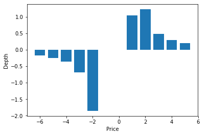
Figure 1: Numerical illustration of a LOB.

3.4 Variance per trade

We provide here the variance per trade (defined previously in Section 2.6) in the case where the tick size is non null. This result is obtained in a similar way as Theorem 2.2.

Theorem 3.2.

The variance per trade $\sigma_{tr}^{2}$ satisfies:

$$\sigma_{tr}^{2}=\mathbb{E}[(P_{\tau_{i+1}}-P_{\tau_{i}})^{2}]=\frac{\mathbb{E}[B^{2}](\mu+\alpha/2)}{\mathbb{E}[|B|\mathbf{1}_{|B|>\mu+\alpha/2}]}.$$ (6)

As in the zero tick size case (see Section 2.6), we consider that the absolute value of the price jumps follows a Pareto distribution and take $x_{0}$ equal to the half spread $\mu+\alpha/2$. The variance per trade becomes:

$$\sigma_{tr}^{2}=\frac{k-1}{k-2}(\mu+\alpha/2)^{2}.$$

We will estimate the scale parameter $k$ from this relationship in Section 5.

3.5 Queue position valuation

Introducing a tick size in our modeling enables us to study the value of the position of the limit orders in the queues. We can quantify the advantage of an order placed on top of a queue compared to another one placed at the bottom. The difference in the values of the positions in a queue is a crucial parameter for trading algorithms. It has actually lead to a technological arms race among high-frequency traders and other automated market participants to establish early (and hence advantageous) positions in the queues, see [2, 27]. Placing limit orders at the front of a queue is very valuable for different reasons. It guarantees early execution and less waiting time. In addition, it reduces adverse selection risk. In fact, as explained in [27], when a limit order is placed at the end of a queue, it is likely that it will be executed against a large trade. In contrast, a limit order placed at the front of the (best) queue will be executed against the next trade independently of the trade size. Large trades are in general sent by informed traders aiming at consuming all limit orders which will generate profit for them. In this way, a limit order submitted at the front of the queue is less likely to undergo adverse selection.

In light of this, to optimize their execution, practitioners need to place limit orders in a relevant way. This requires an estimate of the value of a limit order according to its position in the queue. This very problem is studied in [27] for the queues at the best limits for large tick assets. We complement here this nice work providing formulas valid for any queue of a large or small tick asset and taking into account strategic interactions between market participants.

Assumption 4 tells us that the expected profit of a new infinitesimal limit order placed at the bottom of a non-empty queue is equal to zero. However, under our zero-profit condition, market makers may still make profit if their orders are placed before. The value of queue position at the $i^{th}$ level, denoted by $\tilde{G}^{d}(i)$, can be formulated in this model as the difference between the expected profit of the order placed on top and that of a new one that would be placed at the bottom of the $i^{th}$ queue. Computing this quantity is very similar to deriving the equations in Proposition 3.1. The difference is that now we no longer consider a traded volume totally depleting the limit but a traded volume consuming all the limits before the $i^{th}$ one. This leads to the following theorem.

Theorem 3.3.

For $i\geq k_{r}^{d}$, we have

$$\tilde{G}^{d}(i)=d+(i-1)\alpha-\frac{r\mathbb{E}[B\mathbf{1}_{B>d+(i-1)\alpha}]}{1-rF_{\psi}(d+(i-1)\alpha)-(1-r)F_{\kappa^{u}}\big{(}L^{d}(i-1)\big{)}}.$$

The formula for $i\leq-k_{l}^{d}$ is obviously deduced. We will confront the formula in Theorem 3.3 to data in Section 5.

4 First practical application: Spread forecasting

Our model (in particular Equation (5)) allows us to forecast the new value of the spread if the tick size is modified. In the following, we predict the spread changes due to the new tick size regime under the recent European regulation MiFID II, and compare our results to the effective spread values. We expect our model to be relevant for rather liquid assets since it is based on the presence of competitive market makers. We therefore restrict ourselves to this class. Note that there are other models in the literature enabling practitioners to forecast spreads, see notably [9] where the authors propose an approach designed for large tick assets. This methodology is applied for example in [18] on Japanese data and in [24] where spread values before and after MiFID II are compared. The advantage of our device is that it can be applied on both small and large tick assets.

4.1 The tick size issue and MiFID II regulation

In the recent years, trading platforms have raced to reduce their tick sizes in order to offer better prices and gain market share. This broad trend has had adverse effects on the overall market quality: a too small tick leads to unstable LOBs and a degradation of the price formation mechanism. However, a too large tick prevents the price from moving freely according to the views of market participants. Therefore, finding suitable tick values is crucial for the fluidity of financial markets. To solve this issue, some regulators tried to use pilot programs, as was the case in Japan and in the United States, see for example [18]. This is a costly practice which does not really rely on theoretical foundations. We believe that using quantitative results such as those presented in this work could lead to a much more efficient methodology.

In Europe, MiFID II (Markets in Financial Instruments Directive II) regulation introduced a harmonized tick size regime (Article 49) which is based on a two-entries table: price and liquidity (expressed in terms of number of transactions per day). Note that one of the targets for regulators was to obtain for liquid assets spreads between 1.5 and 2 ticks, see [3].

4.2 Data

Our data are provided by the French regulator Autorité des Marchés Financiers. We study the CAC 40 stocks over a six months time period around the implementation of MiFID II: from October 2017 to December 2017 (before the tick size changes) and from January 2018 to March 2018 (after the tick size changes). We consider assets whose tick size has changed after the implementation of MiFID II regulation. There are 14 stocks from the CAC 40 index then remaining. We note that for all these assets, the tick size was increased.

For each asset we compute two spreads: the first one is averaged over all events occurring in the LOB (transactions, insertions of a new order, cancellations or modifications of an existing order) over the three months before MiFID II and the second one over the three months under MiFID II.

4.3 Prediction of the spread under MiFID II and optimal tick sizes

We now forecast the new spreads of our 14 assets due to the new tick size regime, based on pre-MiFID II data. We use two different predictors. First, we consider that the spread (in euros) remains constant. Second, we compute the new value of the spread based on Equation (5), with $\mu$ estimated on the period from October 2017 to December 2017. We compare the accuracy of our forecasts with respect to the effective spread values in Table 1.

Stock	Tick size before MiF. II	Tick size under MiF. II	Average spread before MiF. II (euros)	Average spread before MiF. II (ticks)	Average spread under MiF. II (euros)	Average spread under MiF. II (ticks)	Expected spread based on our model	Relative error
Safran	0.01	0.02	0.019	1.892	0.031	1.556	0.029	7%
Accor	0.005	0.01	0.011	2.266	0.016	1.586	0.016	3%
Bouygues	0.005	0.01	0.011	2.277	0.017	1.734	0.016	5%
Kering	0.05	0.1	0.090	1.797	0.141	1.407	0.140	1%
Schneider Electric	0.01	0.02	0.016	1.579	0.025	1.235	0.026	4%
Veolia Environnement	0.005	0.01	0.007	1.440	0.012	1.189	0.012	3%
Vinci	0.01	0.02	0.017	1.668	0.026	1.280	0.027	4%
Vivendi	0.005	0.01	0.007	1.408	0.012	1.162	0.012	4%
Publicis	0.01	0.02	0.019	1.904	0.030	1.520	0.029	4%
Legrand	0.01	0.02	0.016	1.643	0.029	1.471	0.026	10%
Valeo	0.01	0.02	0.018	1.845	0.031	1.568	0.028	10%
TechnipFMC	0.005	0.01	0.010	2.056	0.017	1.677	0.015	10%

Table 1: Forecasting CAC 40 assets spreads under MiFID II.

The forecasts based on our model are very accurate: the average relative error is equal to $5\%$ while it is $43\%$ for the other predictor. Remark also that the errors obtained under our methodology are always smaller than the initial tick size, which is almost never the case if one just assumes that the spread in euros is constant.

5 Second practical application: Queue position valuation

As we have seen in Section 3.5, our approach enables us to measure quantitatively the value of queue position thanks to Theorem 3.3. To use this result, we need to know the distribution of $B$. To estimate it, we use the Pareto parametrization of Section 3.4. We will estimate the parameter $k$ from Equation (6) and compute $r$ using Equation (1). Values of queue positions will then be deduced.

5.1 Data

To complement the results of [27], we consider in this section the values of queue position for all small tick stocks of the CAC 40 index (that is stocks for which the average spread is larger than 2 ticks). We study this quantity under MiFID II. These assets are investigated over a three months period: from January 2018 to March 2018. This leaves us with five stocks. We compute on a daily basis the average spread over all events occurring in the LOB and the variance per trade, for each stock.

5.2 Pareto parameters estimation methodology

Under our parametrization, the variance per trade is given by

$$\sigma^{2}_{tr}=\frac{(k-1)(\mu+\alpha/2)^{2}}{k-2}.$$

We estimate $k$ by minimizing for each stock the quadratic error:

$$\sum_{j}\big{(}\sigma_{tr}^{2}-(\widetilde{\sigma_{tr}^{2}})_{j}\big{)}^{2},$$

where $\sigma_{tr}^{2}$ is the variance per trade obtained in our model and $(\widetilde{\sigma_{tr}^{2}})_{j}$ is the variance per trade measured on data (realized variance based on 5 minutes price sampling divided by number of trades) on day $j$. We search for the optimal $k$ between 2.001 and 20. Note that for each stock, the considered spread is equal to the average realized spread during the period under study.

5.3 Queue position valuation

We first report in Table 2 the values of the queue position at the best ask limit according to $d$. We consider that $d$ can be equal to $0.25\alpha$, $0.5\alpha$ or $0.75\alpha$.

Stock	Spread (euros)	Spread (ticks)	k	r	Priority value for $d=0.25\alpha$ (euros)	Priority value for $d=0.25\alpha$ (spreads)	Priority value for $d=0.5\alpha$ (euros)	Priority value for $d=0.5\alpha$ (spreads)	Priority value for $d=0.75\alpha$ (euros)	Priority value for $d=0.75\alpha$ (spreads)
Renault	0.025	2.476	2.866	65%	0.010	41%	0.011	45%	0.012	50%
Lafarge Holcim	0.026	2.438	3.316	70%	0.010	39%	0.011	42 %	0.012	48%
Airbus	0.020	2.040	3.478	71%	0.011	53%	0.012	61%	0.014	68%
Saint-Gobain	0.010	2.035	4.776	79%	0.006	55%	0.007	65%	0.008	76%
Société Generale	0.010	2.012	9.910	90%	0.006	60%	0.007	73%	0.009	86%

Table 2: Queue position values at the best ask according to $d$.

We see that the values of queue position are of the same order of magnitude as the bid-ask spreads. This is in line with the findings in [27]. In addition, we get that it is increasing with $d$. Furthermore, remark that as expected from Section 2.6, the values of $k$ are larger than $2.3$.

We now compute in Table 3 the values of queue position at the four best limits when $d=0.5\alpha$.

Stock	Spread (euros)	Spread (ticks)	k	r	First limit priority value (euros)	First limit priority value (spreads)	Second limit priority value (euros)	Second limit priority value (spreads)	Third limit priority value (euros)	Third limit priority value (spreads)	Fourth limit priority value (euros)	Fourth limit priority value (spreads)
Renault	0.025	2.476	2.866	65%	-0.007	-30%	0.011	45%	0.013	54%	0.013	51%
Lafarge Holcim	0.026	2.438	3.316	70%	-0.008	-31%	0.011	42 %	0.014	55%	0.013	52%
Airbus	0.020	2.040	3.478	71%	-0.005	-25%	0.012	61%	0.015	72%	0.014	67%
Saint-Gobain	0.010	2.035	4.776	79%	-0.003	-25%	0.007	65%	0.009	84%	0.008	78%
Société Generale	0.010	2.012	9.910	90%	-0.003	-25%	0.007	73%	0.012	117%	0.013	127%

Table 3: Queue position values at the four best limits for $d=0.5\alpha$.

Note that the queue position value of the first limit does not necessarily correspond to the best ask. For example, if the priority value at the first limit is negative and the one at the second limit is positive, the best ask is the second limit. We observe that the value of queue position is increasing according to the rank of the limit, up to some level after which it decreases.

Conclusion

In this article, we introduce an agent-based model for the LOB. Inspired by the seminal paper by Glosten and Milgrom [11], we use a zero-profit condition for the market makers which enables us to derive a link between proportion of events due to the noise trader, bid-ask spread, dynamic of the efficient price and equilibrium LOB state. The effect of introducing a tick size is then discussed. We in particular show that the constrained bid-ask spread is equal to the sum of the tick value and the intrinsic bid-ask spread that corresponds to the case of a vanishing tick size. This model allows us to do spread forecasting when one modifies the tick size. Price discreteness also enables us to value queue positions in the LOB.

In our approach, market makers only are allowed to insert limit orders. In practice, the roles of informed trader and market makers are often mixed, and the informed trader also has the possibility to place passive limit orders. By doing so, he may get better prices but also leak some information to other market participants. Extending our model by taking into account accurately these intricate features is left for future work.

Appendix A Proofs

A.1 Proof of Proposition 2.1

We consider the gain of passive sell orders. The gain of passive buy orders can be easily deduced.

First, we compute $G^{inf}(x-\delta p,x)$. We have:

$$G^{inf}(x-\delta p,x) =\int_{x-\delta p}^{x}(P(t)+s)\mathrm{d}\tilde{L}(s)-\int_{x-\delta p}^{x}(P(t)+\mathbb{E}[B|B>x])\mathrm{d}\tilde{L}(s)$$

$$=\int_{x-\delta p}^{x}s\mathrm{d}\tilde{L}(s)-\tilde{L}(x)\mathbb{E}[B|B>x].$$

For $G^{noise}(x-\delta p,x)$ we get:

$$G^{noise}(x-\delta p,x)=\int_{x-\delta p}^{x}(P(t)+s)\mathrm{d}\tilde{L}(s)-\int_{x-\delta p}^{x}P(t)\mathrm{d}\tilde{L}(s)=\int_{x-\delta p}^{x}s\mathrm{d}\tilde{L}(s).$$

We deduce that:

$$G(x-\delta p,x) =G^{inf}(x-\delta p,x)\mathbb{P}[\nu=1|Q\geq L(x)+\tilde{L}(x)]+G^{noise}(x-\delta p,x)\mathbb{P}[\nu=0|Q\geq L(x)+\tilde{L}(x)]$$

$$=\int_{x-\delta p}^{x}s\mathrm{d}\tilde{L}(s)-\mathbb{P}[\nu=1|Q\geq L(x)+\tilde{L}(x)]\tilde{L}(x)\mathbb{E}[B|B>x]$$

$$=\int_{x-\delta p}^{x}s\mathrm{d}\tilde{L}(s)-\tilde{L}(x)\mathbb{E}[B|B>x]\frac{r\mathbb{P}[B>x]}{\mathbb{P}[Q\geq L(x)+\tilde{L}(x)]}$$

$$=\int_{x-\delta p}^{x}s\mathrm{d}\tilde{L}(s)-\tilde{L}(x)\frac{r\mathbb{E}[B\mathbf{1}_{B>x}]}{\mathbb{P}[Q\geq L(x)+\tilde{L}(x)]}$$

$$=\int_{x-\delta p}^{x}s\mathrm{d}\tilde{L}(s)-\tilde{L}(x)\frac{r\mathbb{E}[B\mathbf{1}_{B>x}]}{r\mathbb{P}[B>x]+(1-r)\mathbb{P}[Q^{u}>L(x)+\tilde{L}(x)]}.$$

Integrating by part we get

$$\int_{x-\delta p}^{x}s\mathrm{d}\tilde{L}(s)=\tilde{L}(x)x-\int_{x-\delta p}^{x}\tilde{L}(s)\mathrm{d}s=\varepsilon x-\int_{x-\delta p}^{x}\tilde{L}(s)\mathrm{d}s.$$

When $\delta p$ tends to 0, this tends to $\varepsilon x$. Consequently, we have:

$$\underset{\delta p\rightarrow 0}{\text{lim}}G(x-\delta p,x)=\varepsilon\big{(}x-\frac{r\mathbb{E}[B\mathbf{1}_{B>x}]}{r\mathbb{P}[B>x]+(1-r)\mathbb{P}[Q^{u}>L(x)+\tilde{L}(x)]}\big{)},$$

and

$$G(x)=\underset{\varepsilon\rightarrow 0}{\text{lim}}\big{(}\underset{\delta p\rightarrow 0}{\text{lim}}\frac{G(x-\delta p,x)}{\varepsilon}\big{)}\\ =x-\frac{r\mathbb{E}[B\mathbf{1}_{B>x}]}{r\mathbb{P}[B>x]+(1-r)\mathbb{P}[Q^{u}>L(x)]}.$$

A.2 Proof of Theorem 2.1

We consider the passive sell orders ($x>0$). We first compute $\hat{L}(x)$ which is the theoretical liquidity that market makers should add in the LOB in order to obtain $G(x)=0$. Under Proposition 2.1, $G(x)=0$ is equivalent to:

$$\mathbb{P}[Q^{u}>L(x)] =\frac{r}{1-r}\big{(}\mathbb{E}[\frac{B}{x}\mathbf{1}_{B>x}]-\mathbb{P}[B>x]\big{)}$$

$$=\frac{r}{1-r}\big{(}\mathbb{E}[\frac{B}{x}\mathbf{1}_{B>x}]-1+\mathbb{P}[B<x]\big{)}$$

$$=\frac{r}{1-r}\big{(}-1+\mathbb{E}[\text{max}(\frac{B}{x},1)]\big{)}.$$

We deduce that

$$\hat{L}(x)=F_{\kappa^{u}}^{-1}(\frac{1}{1-r}-\frac{r}{1-r}\mathbb{E}[\text{max}(\frac{B}{x},1)]).$$

We now prove that the spread is positive and finite and deduce the shape of the whole LOB.

Recall that $\hat{L}(x)$ computed above is a theoretical value, and that market makers will add liquidity only when $\hat{L}(x)>0$.

We have $\hat{L}(x)>0$ when ($\frac{1}{1-r}-\frac{r}{1-r}\mathbb{E}[\text{max}(\frac{B}{x},1)])>\frac{1}{2}$. This holds for all $x$ such that $\mathbb{E}[\text{max}(\frac{B}{x},1)]<\frac{1+r}{2r}$. Equivalently, the inequality is satisfied for any $x$ such that $x>\mu$, where $\mu$ is unique solution of the following equation:

$$\mathbb{E}[\text{max}(\frac{B}{\mu},1)]=\frac{1+r}{2r}.$$

By Assumption 2, we deduce that for any $x\leq\mu$, $L(x)=0$. Moreover, for any $x>\mu$,

$$L(x)=F_{\kappa^{u}}^{-1}\big{(}\frac{1}{1-r}-\frac{r}{1-r}\mathbb{E}[\text{max}(\frac{B}{x},1)]\big{)}.$$

We deduce that $\mu$ is the half spread.

The cumulative LOB we obtain is unique, continuous and strictly increasing beyond the spread (since the laws of $B$ and $Q^{u}$ have positive densities on $\mathbb{R}$).

A.3 Proof of Theorem 2.2

We denote by $\nu_{i}$ the random variable that is equal to 1 if the $i^{th}$ trade is initiated by the informed trader and 0 if it is initiated by the noise trader. We write $\omega$ for the number of events between two successive trades. We have:

$$\sigma_{tr}^{2}=\mathbb{E}[(P_{\tau_{i+1}}-P_{\tau_{i}})^{2}]=\sum_{j=1}^{\infty}\mathbb{P}[\omega=j]\mathbb{E}[(P_{\tau_{i+1}}-P_{\tau_{i}})^{2}|\omega=j].$$

with

$$\mathbb{E}[(P_{\tau_{i+1}}-P_{\tau_{i}})^{2}|\omega=j] =\mathbb{P}[\nu_{\tau_{i+1}}=0|\omega=j]\mathbb{E}[(P_{\tau_{i+1}}-P_{\tau_{i}})^{2}|\omega=j,\nu_{\tau_{i+1}}=0]$$

$$+\mathbb{P}[\nu_{\tau_{i+1}}=1|\omega=j]\mathbb{E}[(P_{\tau_{i+1}}-P_{\tau_{i}})^{2}|\omega=j,\nu_{\tau_{i+1}}=1].$$

Knowing that $\omega=j$, the $j^{th}$ event can be a trade initiated by the noise trader or a trade initiated by the informed trader. We have

$$\mathbb{E}[(P_{\tau_{i+1}}-P_{\tau_{i}})^{2}|\omega=j,\nu_{\tau_{i+1}}=1] =\mathbb{E}[(\sum_{k=1}^{j-1}B_{k}+B_{j})^{2}||B_{k}|<\mu,|B_{j}|>\mu]$$

$$=(j-1)\mathbb{E}[B_{k}^{2}||B_{k}|<\mu]+\mathbb{E}[B_{j}^{2}||B_{j}|>\mu].$$

and

$$\mathbb{E}[(P_{\tau_{i+1}}-P_{\tau_{i}})^{2}|\omega=j,\nu_{\tau_{i+1}}=0]=\mathbb{E}[(\sum_{k=1}^{j-1}B_{k})^{2}||B_{k}|<\mu]=(j-1)\mathbb{E}[B_{k}^{2}||B_{k}|<\mu].$$

We compute the probabilities:

$$\mathbb{P}[\nu_{\tau_{i+1}}=1|\omega=j]=\frac{r\mathbb{P}[|B|>\mu]}{1-r\mathbb{P}[|B|<\mu]}$$

and

$$\mathbb{P}[\nu_{\tau_{i+1}}=0|\omega=j]=\frac{1-r}{1-r\mathbb{P}[|B|<\mu]}.$$

Consequently,

$$\sigma_{tr}^{2}=\mathbb{E}[B^{2}||B|\leq\mu]\sum_{j=1}^{\infty}(j-1)\mathbb{P}[\omega=j]+\mathbb{E}[B^{2}||B|>\mu]\frac{r\mathbb{P}[|B|>\mu]}{1-r\mathbb{P}[|B|<\mu]}.$$

We have:

$$\sum_{j=1}^{\infty}\mathbb{P}[\omega=j](j-1) =(1-r\mathbb{P}[|B|<\mu])\sum_{j=1}^{\infty}(j-1)(r\mathbb{P}[|B|<\mu])^{j-1}$$

$$=(1-r\mathbb{P}[|B|<\mu])\sum_{j=0}^{\infty}j(r\mathbb{P}[|B|<\mu])^{j}$$

$$=\frac{r\mathbb{P}[|B|<\mu]}{\big{(}1-r\mathbb{P}[|B|<\mu]\big{)}}.$$

We deduce:

$$\sigma_{tr}^{2}=\frac{r\mathbb{E}[B^{2}\mathbf{1}_{|B|<\mu}]+r\mathbb{E}[B^{2}\mathbf{1}_{|B|>\mu}]}{1-r\mathbb{P}[|B|\leq\mu]}\\ =\frac{r\mathbb{E}[B^{2}]}{1-r\mathbb{P}[|B|\leq\mu]}.$$

Recall that from Equation (1) :

$$\frac{1+r}{2r}=\mathbb{E}[\text{max}(\frac{B}{\mu},1)]=\mathbb{E}[\frac{B}{\mu}\mathbf{1}_{B>\mu}]+\mathbb{P}[B\leq\mu].$$

this implies that

$$\frac{1+r}{r}-1=\mathbb{E}\left[\frac{|B|}{\mu}\mathbf{1}_{|B|>\mu}\right]+\mathbb{P}[|B|\leq\mu].$$

Thus we conclude that

$$\sigma_{tr}^{2}=\frac{\mathbb{E}[B^{2}]\mu}{\mathbb{E}[|B|\mathbf{1}_{|B|>\mu}]}.$$

A.4 Proof of Proposition 3.1

We just give a sketch of proof here since the computations are essentially the same as for the proof of Proposition 2.1. In particular, we do not introduce the volume $\varepsilon$ of limit orders and directly work in the asymptotic regime $\varepsilon$ tending to zero. We consider the gain of passive sell orders. The gain of passive buy orders can be deduced the way.

First, we compute the gain of a new order placed at the $i^{th}$ limit when the trade is initiated by an informed trader, knowing that $Q^{i}>L^{d}(i)$, denoted by $G^{d}_{inf}(i)$:

$$G^{d}_{inf}(i)=d+(i-1)\alpha-\mathbb{E}[B|B>d+(i-1)\alpha].$$

Second, we compute the gain of a new order placed at the $i^{th}$ limit when the trade is initiated by a noise trade, knowing that $Q^{i}>L^{d}(i)$, denoted by $G^{d}_{noise}(i)$:

$$G^{d}_{noise}(i)=d+(i-1)\alpha.$$

Now, $G^{d}(i)$ satisfies:

$$G^{d}(i) =G^{d}_{inf}(i)\mathbb{P}[\nu=1|Q>L^{d}(i)]+G^{d}_{noise}(i)\mathbb{P}[\nu=0|Q>L^{d}(i)]$$

$$=d+(i-1)\alpha-\frac{r\mathbb{E}[B\mathbf{1}_{B>d+(i-1)\alpha}]}{\mathbb{P}[Q>L(d+(i-1)\alpha])}$$

$$=d+(i-1)\alpha-\frac{r\mathbb{E}[B\mathbf{1}_{B>d+(i-1)\alpha}]}{r\mathbb{P}[B>d+(i-1)\alpha]+(1-r)\mathbb{P}[Q^{u}>L(d+(i-1)\alpha)]}.$$

A.5 Proof of Theorem 3.1

We consider the ask side. First we show that the spread is positive and finite. Then we prove that beyond the spread, market makers insert limit orders on all possible limit prices.

We showed in the case where the tick size is null that there exists $\mu$ such that for all $x\leq\mu,L(x)=0$ and for all $x>\mu,L(x)>0$. The LOB being now discrete, the previous findings remain true for $k_{r}^{d}$ instead of $\mu$ where $k_{r}^{d}$ satisfies:

$$k_{r}^{d}=\text{min}\{k\in\mathbb{N}^{+}|d+(k-1)\alpha>\mu\}.$$

So we have:

$$k_{r}^{d}=1+\lceil\frac{\mu-d}{\alpha}\rceil.$$

Similarly, for the first non-empty limit at the bid side, we get:

$$k_{l}^{d}=\lceil\frac{\mu+d}{\alpha}\rceil.$$

From Equation (4), the spread is equal to $(k_{r}^{d}+k_{l}^{d})\alpha-\alpha$. Thus the conditional constrained bid-ask spread $\phi_{\alpha}^{d}$, given the value of $d$, satisfies:

$$\phi_{\alpha}^{d}=\alpha(\lceil\frac{\mu-d}{\alpha}\rceil+\lceil\frac{\mu+d}{\alpha}\rceil).$$

Under Assumption 4, we have for any $i\geq k_{r}^{d}$:

$$L(d+(i-1)\alpha)=F_{\kappa^{u}}^{-1}(\frac{1}{1-r}-\frac{r}{1-r}\mathbb{E}[\text{max}(\frac{B}{d+(i-1)\alpha},1)]).$$

We deduce that the cumulative LOB is unique and increasing beyond the spread.

A.6 Proof of Corollary 3.1

The parameter $d$ being approximately uniformly distributed between $[0,\alpha)$, we can compute the average value of the constrained bid-ask spread by integrating $\phi_{\alpha}^{d}$:

$$\phi_{\alpha}=\int_{0}^{\alpha}\lceil\frac{\mu-s}{\alpha}\rceil+\lceil\frac{\mu+s}{\alpha}\rceil\text{d}s.$$

Denote $u:=\frac{\mu}{\alpha}$. We have:

$$\phi_{u}=\alpha\int_{0}^{1}\lceil u-x\rceil+\lceil u+x\rceil\text{d}x.$$

We decompose $u$ such that $u=u_{i}+u_{f}$, where $u_{i}$ represents the integer part of $u$. We get:

$$\phi_{\alpha}=\alpha\int_{0}^{1}\lceil u_{i}+u_{f}-x\rceil+\lceil u_{i}+u_{f}+x\rceil\text{d}x.$$

$$\phi_{\alpha}=\alpha\big{(}\int_{0}^{u_{f}}(u_{i}+1)\text{d}x+\int_{u_{f}}^{1}u_{i}\text{d}x+\int_{0}^{1-u_{f}}(u_{i}+1)\text{d}x+\int_{(1-u_{f})}^{1}(u_{i}+2)\text{d}x\big{)}.$$

$$\phi_{\alpha}=\alpha\big{(}u_{f}(u_{i}+1)+(1-u_{f})u_{i}+(1-u_{f})(u_{i}+1)+u_{f}(u_{i}+2)\big{)}.$$

$$\phi_{\alpha}=\alpha(2u_{i}+2u_{f}+1)=\alpha+2\mu=\alpha+\phi.$$

References

- [1] Frédéric Abergel and Aymen Jedidi. A mathematical approach to order book modeling. International Journal of Theoretical and Applied Finance, 16(05):1350025, 2013.
- [2] Frédéric Abergel, Charles-Albert Lehalle, and Mathieu Rosenbaum. Understanding the stakes of high-frequency trading. The Journal of Trading, 9(4):49–73, 2014.
- [3] Autorité des Marchés Financiers. MiFID II: Impact of the new tick size regime. AMF report, 2018.
- [4] Shmuel Baruch and Lawrence R Glosten. Tail expectation, imperfect competition, and the phenomenon of flickering quotes in limit order book markets. Unpublished Manuscript, David Eccles School of Business, University of Utah, 2017.
- [5] Christian Bayer, Ulrich Horst, and Jinniao Qiu. A functional limit theorem for limit order books with state dependent price dynamics. The Annals of Applied Probability, 27(5):2753–2806, 2017.
- [6] Dan Bernhardt and Eric Hughson. Splitting orders. The Review of Financial Studies, 10(1):69–101, 1997.
- [7] Rama Cont and Adrien De Larrard. Price dynamics in a Markovian limit order market. SIAM Journal on Financial Mathematics, 4(1):1–25, 2013.
- [8] Rama Cont, Sasha Stoikov, and Rishi Talreja. A stochastic model for order book dynamics. Operations Research, 58(3):549–563, 2010.
- [9] Khalil Dayri and Mathieu Rosenbaum. Large tick assets: implicit spread and optimal tick size. Market Microstructure and Liquidity, 1(01):1550003, 2015.
- [10] Thierry Foucault. Order flow composition and trading costs in a dynamic limit order market. Journal of Financial Markets, 2(2):99–134, 1999.
- [11] Lawrence R Glosten and Paul R Milgrom. Bid, ask and transaction prices in a specialist market with heterogeneously informed traders. Journal of Financial Economics, 14(1):71–100, 1985.
- [12] Martin D Gould, Mason A Porter, Stacy Williams, Mark McDonald, Daniel J Fenn, and Sam D Howison. Limit order books. Quantitative Finance, 13(11):1709–1742, 2013.
- [13] Takaki Hayashi and Yuta Koike. Wavelet-based methods for high-frequency lead-lag analysis. SIAM Journal on Financial Mathematics, 9(4):1208–1248, 2018.
- [14] Thomas Ho and Hans R Stoll. Optimal dealer pricing under transactions and return uncertainty. Journal of Financial Economics, 9(1):47–73, 1981.
- [15] Marc Hoffmann, Mathieu Rosenbaum, and Nakahiro Yoshida. Estimation of the lead-lag parameter from non-synchronous data. Bernoulli, 19(2):426–461, 2013.
- [16] Roger D Huang and Hans R Stoll. The components of the bid-ask spread: A general approach. The Review of Financial Studies, 10(4):995–1034, 1997.
- [17] Weibing Huang, Charles-Albert Lehalle, and Mathieu Rosenbaum. Simulating and analyzing order book data: The queue-reactive model. Journal of the American Statistical Association, 110(509):107–122, 2015.
- [18] Weibing Huang, Charles-Albert Lehalle, and Mathieu Rosenbaum. How to predict the consequences of a tick value change? Evidence from the Tokyo Stock Exchange pilot program. Market Microstructure and Liquidity, 2(03n04):1750001, 2016.
- [19] Weibing Huang and Mathieu Rosenbaum. Ergodicity and diffusivity of Markovian order book models: a general framework. SIAM Journal on Financial Mathematics, 8(1):874–900, 2017.
- [20] Nicolas Huth and Frédéric Abergel. High frequency lead/lag relationships: Empirical facts. Journal of Empirical Finance, 26:41–58, 2014.
- [21] P Kosulajeff. Sur la répartition de la partie fractionnaire d’une variable. Matematiceskij Sbornik, 2(5):1017–1019, 1937.
- [22] Albert S Kyle. Continuous auctions and insider trading. Econometrica: Journal of the Econometric Society, pages 1315–1335, 1985.
- [23] Aimé Lachapelle, Jean-Michel Lasry, Charles-Albert Lehalle, and Pierre-Louis Lions. Efficiency of the price formation process in presence of high frequency participants: a mean field game analysis. Mathematics and Financial Economics, 10(3):223–262, 2016.
- [24] Sophie Laruelle, Mathieu Rosenbaum, and Emel Savku. Assessing MiFID II regulation on tick sizes: A transaction costs analysis viewpoint. Working Paper, 2018.
- [25] Ananth Madhavan, Matthew Richardson, and Mark Roomans. Why do security prices change? A transaction-level analysis of NYSE stocks. The Review of Financial Studies, 10(4):1035–1064, 1997.
- [26] Nicolas Megarbane, Pamela Saliba, Charles-Albert Lehalle, and Mathieu Rosenbaum. The behavior of high-frequency traders under different market stress scenarios. Market Microstructure and Liquidity, page 1850005, 2017.
- [27] Ciamac C Moallemi and Kai Yuan. A model for queue position valuation in a limit order book. Working paper, 2016.
- [28] Christine A Parlour. Price dynamics in limit order markets. The Review of Financial Studies, 11(4):789–816, 1998.
- [29] Mathieu Rosenbaum. Integrated volatility and round-off error. Bernoulli, 15(3):687–720, 2009.
- [30] Ioanid Roşu. A dynamic model of the limit order book. The Review of Financial Studies, 22(11):4601–4641, 2009.
- [31] Eric Smith, J Doyne Farmer, Laszlo Gillemot, and Supriya Krishnamurthy. Statistical theory of the continuous double auction. Quantitative finance, 3(6):481–514, 2003.
- [32] John Wilder Tukey. On the distribution of the fractional part of a statistical variable. Matematiceskij Sbornik, 4(3):561–562, 1938.
- [33] Matthieu Wyart, Jean-Philippe Bouchaud, Julien Kockelkoren, Marc Potters, and Michele Vettorazzo. Relation between bid–ask spread, impact and volatility in order-driven markets. Quantitative Finance, 8(1):41–57, 2008.