Abstract.

We consider smooth solutions of the wave equation, on a fixed black hole region of a subextremal Reissner-Nordström (asymptotically flat, de Sitter or anti-de Sitter) spacetime, whose restrictions to the event horizon have compact support. We provide criteria, in terms of surface gravities, for the waves to remain in $C^{l}$, $l\geqslant 1$, up to and including the Cauchy horizon. We also provide sufficient conditions for the blow up of solutions in $C^{1}$ and $H^{1}$.

1. Introduction

Cauchy horizons are the spacetime boundary of the maximal Cauchy development of initial value problems for the Einstein field equations. Whenever non-empty, their existence and stability puts into question global uniqueness, and consequently challenges the deterministic character of General Relativity. To understand how perturbations of a static charged black hole behave at the Cauchy horizon that lies in its interior, we will study solutions of the wave equation on the black hole region of fixed subextremal Reissner-Nordström (asymptotically flat, de Sitter or anti-de Sitter) spacetimes. In this framework, it is natural to consider that Cauchy horizons that allow solutions with higher regularity are more stable than the ones that do not.

The stability of Cauchy horizons is a classical problem in General Relativity and, in recent years, considerable progress has been made in its understanding through the mathematical analysis of wave equations. Stability results can be found in [12, 24, 3, 13, 14, 19, 16, 17] and instability results in [20, 23, 9, 10], and the references therein. For developments concerning the analysis of the full Einstein equations we refer to [4, 5, 6, 7, 21, 22, 8, 25].

Most of the literature about the linear problem focuses on stability-regularity at the $C^{0}$ and $H^{1}$ levels, in line with the modern formulations of the Strong Cosmic Censorship Conjecture. There are however some notable exceptions. In [13], Gajic provides criteria for the $C^{1}$ and $C^{2}$ extendibility of spherically symmetric waves on (asymptotically flat) extremal black holes. In the subextremal de Sitter setting, Hintz and Vasy [17] have shown that solutions of the wave equation arising from smooth Cauchy data have $H^{1/2+\alpha/\kappa_{-}-\epsilon}$ regularity up to the Cauchy horizon, with the degree of regularity being dictated by $\alpha$, the spectral gap of the operator $\Box_{g}$ (which also controls the decay rate of solutions along the event horizon), and $\kappa_{-}$, the Cauchy horizon’s surface gravity. However, recent numerical computations of the spectral gap [2] suggest that the regularity never exceeds $H^{3/2-\epsilon}$.

Here we present criteria for higher order linear stability of the Cauchy horizon, meaning $C^{l}$ with $l\geqslant 1$, in a subextremal Reissner-Nordström spacetime, as well as criteria for linear instability, in both $C^{1}$ and $H^{1}$. We will achieve this by considering waves, without symmetry assumptions, whose restrictions to the event horizon have compact support. Although, in view of the results in [11, 1, 18], this behavior on the event horizon cannot arise from generic Cauchy data, it provides a class of bona fide characteristic initial value problems for the wave equation. We will show that an arbitrarily high regularity at the Cauchy horizon can be obtained by increasing the order to which the wave vanishes in a direction transverse to the event horizon. Moreover, for this initial value problem, the role of the surface gravities in determining the degree of stability of the Cauchy horizon becomes particularly transparent. For instance, we will prove that, as a consequence of a well known relation between surface gravities, if the wave only vanishes to zeroth order at the event horizon then, in spite of having compact support on the event horizon, it cannot be extended in $C^{1}$ to any neighborhood of any point on the Cauchy horizon. In particular, this shows that we cannot expect to obtain arbitrarily high regularity for waves up to and including the Cauchy horizon by simply increasing their decay rate along the event horizon.

1.1. Statement of the main results

Let us set some basic terminology and notation. Let $({\cal M},g)$ be a connected component of the black hole region of a subextremal Reissner-Nordström (asymptotically flat, de Sitter or anti-de Sitter) spacetime. Denote by $\kappa_{+}$ and $\kappa_{-}$ the surface gravities of the future event horizon $\cal{H}^{+}$ and the future Cauchy horizon $\cal{CH}^{+}$, respectively, and let ${\cal H}_{A}^{+}$ and $\cal{CH}_{A}^{+}$ denote the “right side” components of these horizons (see Figure 1). Let $v$ be a future increasing affine parameter of the generators of ${\cal H}_{A}^{+}$, constant on each symmetry sphere, and let $\underline{\cal C}_{v_{0}}$ denote an ingoing null hypersurface that intersects ${\cal H}_{A}^{+}$, at $v=v_{0}$. Letting $X$ be a smooth vector field which is tangent to $\underline{\cal C}_{v_{0}}$ and transverse to ${\cal H}_{A}^{+}$, we will say that $\phi|_{\underline{\cal C}_{v_{0}}}$ vanishes to order $s\in\mathbb{Z}_{0}^{+}$ at ${\cal H}^{+}$ if

$$\phi|_{\underline{\cal C}_{v_{0}}\cap\,{\cal H}^{+}}=(X\phi)|_{\underline{\cal C}_{v_{0}}\cap\,{\cal H}^{+}}=\cdots=(X^{s}\phi)|_{\underline{\cal C}_{v_{0}}\cap\,{\cal H}^{+}}=0.$$ (1)

We are interested in properties of functions that belong to the space

$$\cal{F}_{s} := \{\phi\in C^{\infty}({\cal M}\cup{\cal H}^{+}):\Box_{g}\phi=0,$$ (2)

$$\ \ \phi|_{\cal{H}^{+}\cap\{v\geqslant v_{0}\}}=0,\ \phi|_{\underline{\cal C}_{v_{0}}}\ \mbox{vanishes to order}\ s\ \mbox{at}\ \cal{H}^{+}\},$$

for a fixed $s\in\mathbb{Z}^{+}_{0}$ and some $v_{0}\in\mathbb{R}$.

We may now state our four main theorems. In all of them $s$ belongs to $\mathbb{Z}^{+}_{0}$.

Theorem 1.1.

If $\phi\in\cal{F}_{s}$ and $(s+1)\kappa_{+}>\kappa_{-}$, then $\phi$ belongs to $C^{1}({\cal M}\cup\cal{CH}_{A}^{+})$. Moreover, the second mixed null derivatives of $\phi$ belong to $C^{0}({\cal M}\cup\cal{CH}_{A}^{+})$, the restriction of $\phi$ to symmetry spheres is $C^{2}$, and $\phi$ satisfies the wave equation on the Cauchy horizon.

Theorem 1.2.

Let $l\geqslant 1$. If $\phi\in\cal{F}_{s}$ and $(s+1)\kappa_{+}>l\kappa_{-}$, then $\phi$ belongs to $C^{l}({\cal M}\cup\cal{CH}_{A}^{+})$.

Theorem 1.3.

If the spherical mean of $\phi$ (see (35)) belongs to $\cal{F}_{s}\setminus\cal{F}_{s+1}$ and $(s+1)\kappa_{+}<\kappa_{-}$, then $\phi$ does not belong to $C^{1}(({\cal M}\cup\cal{CH}_{A}^{+})\cap{\cal U})$, for any open set ${\cal U}\cap\cal{CH}_{A}^{+}\neq\emptyset$.

Since the inequality $\kappa_{+}<\kappa_{-}$ is valid in the entire subextremal range of Reissner-Nordström we conclude that, if $\phi\in\cal{F}_{0}\setminus\cal{F}_{1}$, then it cannot be extended in $C^{1}$ to any neighborhood of any point on the Cauchy horizon.

It is an easy consequence of [24] that if $\phi\in\cal{F}_{s}$ with $2(s+1)\kappa_{+}>\kappa_{-}$, then $\phi$ belongs to $H^{1}_{{\rm loc}}(\cal{M}\cup\cal{CH}_{A}^{+})$. We prove that this result is essentially sharp.

Theorem 1.4.

If the spherical mean of $\phi$ belongs to $\cal{F}_{s}\setminus\cal{F}_{s+1}$ with $2(s+1)\kappa_{+}<\kappa_{-}$, then $\phi$ does not belong to $H^{1}(({\cal M}\cup\cal{CH}_{A}^{+})\cap{\cal U})$, for any open set ${\cal U}\cap\cal{CH}_{A}^{+}\neq\emptyset$.

The organization of this paper is as follows. In Section 2 we explain the basic setup of our problem. In Section 3 we recall three energy estimates due to Sbierski. In Section 4 we upgrade the previous to pointwise estimates. In Section 5 we prove Theorem 1.1 which establishes the existence of a classical solution up to and including the Cauchy horizon. In Section 6 we prove Theorem 1.2 concerning solutions with higher regularity. Finally, in Section 7 we prove Theorems 1.3 and 1.4 about blow up in $C^{1}$ and in $H^{1}$.

2. Setup

2.1. Some useful coordinate systems.

We will study solutions of the wave equation on a fixed background consisting of the black hole region of a subextremal Reissner-Nordström (asymptotically flat, de Sitter or anti-de Sitter) spacetime. This spacetime has a metric given in a local coordinate system by

$$g = -D\,dt^{2}+\frac{1}{D}\,dr^{2}+r^{2}\sigma_{\mathbb{S}^{2}},$$

where $\sigma_{\mathbb{S}^{2}}=d\theta^{2}+\sin^{2}\theta\,d\varphi^{2}$ is the round metric on the $2$-sphere, and

$$D=D(r)=1-\,\frac{2m}{r}+\frac{e^{2}}{r^{2}}-\,\frac{\Lambda}{3}r^{2}.$$

Here $m>0$ is the mass, $e\neq 0$ is the charge parameter and $\Lambda\in\mathbb{R}$ is the cosmological constant. We will assume that the function $D$ has at least two positive roots, the smallest of which are

$$0<r_{-}<r_{+}.$$

The values $r_{-}$ and $r_{+}$ correspond to the values of $r$ at the Cauchy horizon $\cal{CH}^{+}$ and at the event horizon ${\cal H}^{+}$, respectively. The Penrose diagram of this spacetime for positive $\Lambda$ is given in Figure 1.

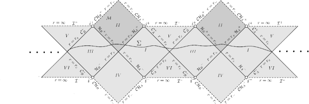
Figure 1. The Penrose diagram of the Reissner-Nordström-de Sitter spacetime.

The surface gravities of the Cauchy and event horizons, defined by

$$\kappa_{-}=\frac{1}{2}|D^{\prime}(r_{-})|\quad\text{and}\quad\kappa_{+}=\frac{1}{2}|D^{\prime}(r_{+})|,$$ (3)

are of fundamental importance to us here. Throughout we will assume that the surface gravities do not vanish, which restricts the scope of our analysis to the subextremal setting.

For $r\in[r_{-},r_{+}]$, we have

$$D(r)=-e^{O(1)}{(r-r_{-})(r_{+}-r)}.$$ (4)

Moreover, any tortoise coordinate

$$\frac{dr^{*}}{dr}=\frac{1}{D}$$

satisfies, for $r\in\,]r_{-},r_{+}[$,

$$r^{*}(r)=-\frac{1}{2\kappa_{-}}\ln|r-r_{-}|+\frac{1}{2\kappa_{+}}\ln|r-r_{+}|+O(1).$$ (5)

The black hole region corresponds to

$$(t,r,\omega)\in{\cal M}:=\,]-\infty,+\infty[\times]r_{-},r_{+}[\times\mathbb{S}^{2},$$

a region where the function $D$ is negative, and where $r^{*}$ varies in $]-\infty,+\infty[$.

We will often rely on the double null coordinates $(\underline{u},\underline{v})\in\,]-\infty,+\infty[^{2}$ given in terms of $t$ and $r$ by

$$\begin{cases}\underline{u}=t-r^{*}(r),\\ \underline{v}=t+r^{*}(r).\end{cases}$$

In these coordinates the metric takes the form

$$g = -D\,d\underline{u}d\underline{v}+r^{2}\sigma_{\mathbb{S}^{2}}.$$

Clearly, we have

$$r^{*}(r)=\frac{\underline{v}-\underline{u}}{2}.$$ (6)

Note that the event horizon corresponds to $\underline{u}=+\infty$ and the Cauchy horizon corresponds to $\underline{v}=+\infty$. Since our double null coordinates are singular at these horizons, at the event horizon we change from $(\underline{u},\underline{v},\omega)$ coordinates to $(v,r,\omega)$ coordinates using

$$\begin{cases}\underline{u}=v-2r^{*}(r),\\ \underline{v}=v,\end{cases}\qquad\begin{cases}\partial_{\underline{u}}=-\,\frac{D}{2}\partial_{r},\\ \partial_{\underline{v}}=\partial_{v}+\frac{D}{2}\partial_{r}.\end{cases}$$

In these coordinates the metric becomes

$$g=-D\,dv^{2}+2\,dvdr+r^{2}\sigma_{\mathbb{S}^{2}}.$$

At the Cauchy horizon we change from $(\underline{u},\underline{v},\omega)$ coordinates to $(u,\tilde{r},\omega)$ coordinates using

$$\begin{cases}\underline{u}=u,\\ \underline{v}=u+2r^{*}(\tilde{r}),\end{cases}\qquad\begin{cases}\partial_{\underline{u}}=\partial_{u}-\,\frac{D}{2}\partial_{\tilde{r}},\\ \partial_{\underline{v}}=\frac{D}{2}\partial_{\tilde{r}}.\end{cases}$$

In these coordinates the metric is written as

$$g=-D\,du^{2}-2\,dud\tilde{r}+r^{2}\sigma_{\mathbb{S}^{2}}.$$

Note that to change from $(v,r,\omega)$ coordinates to $(u,\tilde{r},\omega)$ coordinates we can use

$$\begin{cases}u=v-2r^{*}(r),\\ \tilde{r}=r,\end{cases}\qquad\begin{cases}\partial_{u}=\partial_{v},\\ \partial_{\tilde{r}}=\frac{2}{D}\partial_{v}+\partial_{r}.\end{cases}$$

By abuse of notation, we will write $\phi(\underline{u},\underline{v},\omega)=\phi(v,r,\omega)=\phi(u,r,\omega)$.

It is important to note that the vector field $\partial_{t}=\partial_{v}=\partial_{u}$ is Killing. We also denote by ${\it\Omega}_{i}$, for $i=1,2,3$, the generators of spherical symmetry, and just by ${\it\Omega}$ any one of the three. The vector fields ${\it\Omega}$ are also Killing.

2.2. The wave equation

Define

$$G_{n}=\frac{1}{r}D+\frac{n}{2}D^{\prime},$$ (7)

$$S=-\,\frac{1}{r}\partial_{v}-\frac{1}{2}\not{\Delta}\qquad\mbox{and}\qquad\tilde{S}=\frac{1}{r}\partial_{u}-\frac{1}{2}\not{\Delta},$$ (8)

with $\not{\Delta}\phi$ denoting the spherical laplacian of $\phi$,

$$\not{\Delta}\phi=\frac{1}{r^{2}}\partial_{\theta}^{2}\phi+\frac{1}{r^{2}}\cot\theta\,\partial_{\theta}\phi+\frac{1}{r^{2}\sin^{2}\theta}\partial_{\varphi}^{2}\phi.$$

The wave equation,

$$\Box_{g}\phi=\nabla^{\mu}\nabla_{\mu}\phi=0,$$

is equivalent to both

$$\partial_{\underline{v}}\partial_{r}\phi+G_{1}\partial_{r}\phi=S(\phi)$$ (9)

and

$$\partial_{\underline{u}}\partial_{\tilde{r}}\phi-G_{1}\partial_{\tilde{r}}\phi=-\tilde{S}(\phi).$$ (10)

2.3. The energy-momentum tensor

Recall that to a scalar function $\phi$ we may associate the energy-momentum tensor

$$T_{\mu\nu}=\partial_{\mu}\phi\partial_{\nu}\phi-\frac{1}{2}g_{\mu\nu}(\partial_{\alpha}\phi\,\partial^{\alpha}\phi),$$

whose relevance for the study of solutions of the wave equation stems from the fact that its divergence satisfies

$$\nabla^{\mu}T_{\mu\nu}=(\Box_{g}\phi)\,\partial_{\nu}\phi.$$

Our energy estimates for $\phi$ will be obtained by applying the Divergence Theorem to certain currents, which are contractions of the energy-momentum tensor with appropriate vector fields. It will be useful to have the expression of the energy-momentum tensor in coordinates. One readily checks that

$$\begin{cases}T(\partial_{\underline{u}},\partial_{\underline{u}})=(\partial_{\underline{u}}\phi)^{2},\\ T(\partial_{\underline{u}},\partial_{\underline{v}})=\frac{D}{4}|\not{\nabla}\phi|^{2},\\ T(\partial_{\underline{v}},\partial_{\underline{v}})=(\partial_{\underline{v}}\phi)^{2}.\end{cases}$$

Again, $\not{\nabla}\phi$ denotes the spherical gradient of $\phi$,

$$\not{\nabla}\phi=\frac{1}{r^{2}}(\partial_{\theta}\phi)\,\partial_{\theta}+\frac{1}{r^{2}\sin^{2}\theta}(\partial_{\varphi}\phi)\,\partial_{\varphi},$$

and

$$|\not{\nabla}\phi|^{2}=r^{2}\sigma_{\mathbb{S}^{2}}(\not{\nabla}\phi,\not{\nabla}\phi).$$

2.4. Energy identities and the Divergence Theorem

We will apply the Divergence Theorem in regions bounded by hypersurfaces $\underline{\cal C}_{v}$, where $\underline{v}$ is constant equal to $v$, hypersurfaces ${\cal C}_{u}$, where $\underline{u}$ is constant equal to $u$, and hypersurfaces $\Sigma_{r}$, where the geometric variable $r$ is constant equal to $r$. Denoting by $n_{\underline{\cal C}_{v}}$, $n_{{\cal C}_{u}}$ and $n_{\Sigma_{r}}$ the corresponding normals, with $n_{\Sigma_{r}}$ unit and all three future directed, and denoting by $dV_{\underline{\cal C}_{v}}$, $dV_{{\cal C}_{u}}$ and $dV_{\Sigma_{r}}$ the corresponding volume elements, we have

$$\begin{array}[]{rclcrcl}n_{\underline{\cal C}_{v}}&=&-\partial_{r},&&dV_{{\underline{\cal C}_{v}}}&=&r^{2}\,drd\omega,\\ \vspace{-3mm}\hfil\\ n_{{\cal C}_{u}}&=&-\partial_{\tilde{r}},&&dV_{{\cal C}_{u}}&=&r^{2}\,d\tilde{r}d\omega,\\ \vspace{-3mm}\hfil\\ n_{\Sigma_{r}}&=&\frac{-\partial_{u}+D\partial_{\tilde{r}}}{\sqrt{-D}},&&dV_{\Sigma_{r}}&=&\sqrt{-D}\,r^{2}\,dud\omega,\end{array}$$

where $d\omega$ is the volume form associated to $\sigma_{\mathbb{S}^{2}}$. Note that along the null hypersurfaces there is no natural choice of normal or volume form, so one can just choose a convenient normal and then let the Divergence Theorem determine the volume form.

Our currents will be vector fields of the form

$$J^{N}_{\nu}=J^{N}_{\nu}(\phi):=T_{\mu\nu}N^{\mu}=T_{\mu\nu}(\phi)N^{\mu},$$

with $N$ timelike and future pointing, so that if $\phi$ is a solution of the wave equation, then

$$\nabla^{\nu}J^{N}_{\nu} = (\nabla^{\nu}T_{\mu\nu})N^{\mu}+T_{\mu\nu}\nabla^{\nu}N^{\mu}$$

$$= (\Box_{g}\phi)\,N\cdot\phi+T_{\mu\nu}\nabla^{\nu}N^{\mu}=T_{\mu\nu}\nabla^{\nu}N^{\mu}.$$

Our choices of $N$ will be such that $T_{\mu\nu}\nabla^{\nu}N^{\mu}$ is nonnegative. We denote by

$${\cal C}_{u}(r_{2},r_{1})={\cal C}_{u}\cap\{r_{2}\leqslant r\leqslant r_{1}\},$$

$${\underline{\cal C}}_{v}(r_{2},r_{1})={\underline{\cal C}}_{v}\cap\{r_{2}\leqslant r\leqslant r_{1}\}.$$

Applying the Divergence Theorem to the current $J^{N}_{\nu}$ in the region

$${\cal R}=\{u\geqslant u_{0}\wedge v\leqslant v_{0}\wedge r_{2}\leqslant r\leqslant r_{1}\}$$

Figure 2. The region $\cal{R}$.

(see Figure 2) we get the energy identity

$$\int\displaylimits_{\Sigma_{r_{1}}\cap\{u\geqslant u_{0}\wedge v\leqslant v_{0}\}}J^{N}_{\nu}n^{\nu}_{\Sigma_{r_{1}}}\,dV_{\Sigma_{r_{1}}}-\int\displaylimits_{\underline{\cal C}_{v_{0}}(r_{2},r_{1})}J^{N}_{\nu}n^{\nu}_{\underline{\cal C}_{v_{0}}}\,dV_{\underline{\cal C}_{v_{0}}}\qquad\qquad$$

$$-\int\displaylimits_{\cal{C}_{u_{0}}(r_{2},r_{1})}J^{N}_{\nu}n^{\nu}_{\cal{C}_{u_{0}}}\,dV_{\cal{C}_{u_{0}}}-\int\displaylimits_{\Sigma_{r_{2}}\cap\{u\geqslant u_{0}\wedge v\leqslant v_{0}\}}J^{N}_{\nu}n^{\nu}_{\Sigma_{r_{2}}}\,dV_{\Sigma_{r_{2}}}\qquad\qquad$$

$$=\iint\displaylimits_{\cal{R}}\nabla^{\nu}J^{N}_{\nu}\,dV_{\cal{M}}.$$

For a hypersurface $S$, the integral

$$\int_{S}J^{N}_{\nu}n^{\nu}_{S}\,dV_{S}=\int_{S}T(N,n_{S})\,dV_{S}$$

controls first order derivatives of $\phi$. Let us give an example by defining, near the Cauchy horizon, $N=\tilde{N}_{b}=-\partial_{\underline{u}}-\partial_{\tilde{r}}$. This choice leads to

$$T(\tilde{N}_{b},n_{\underline{\cal C}_{v}})\,dV_{\underline{\cal C}_{v}} = \left(-\,\frac{2}{D}T(\partial_{\underline{u}},\partial_{\underline{u}})-\,\frac{4}{D^{2}}T(\partial_{\underline{u}},\partial_{\underline{v}})\right)r^{2}\,drd\omega$$

$$= \left[-\,\frac{1}{D}\left(2(\partial_{\underline{u}}\phi)^{2}+|\not{\nabla}\phi|^{2}\right)\right]r^{2}\,drd\omega,$$

$$T(\tilde{N}_{b},n_{{\cal C}_{u}})\,dV_{{\cal C}_{u}} = \left(\frac{2}{D}T(\partial_{\underline{u}},\partial_{\underline{v}})+\frac{4}{D^{2}}T(\partial_{\underline{v}},\partial_{\underline{v}})\right)r^{2}\,d\tilde{r}d\omega$$

$$= \left[(\partial_{\tilde{r}}\phi)^{2}+\frac{1}{2}|\not{\nabla}\phi|^{2}\right]r^{2}\,d\tilde{r}d\omega,$$

$$T(\tilde{N}_{b},n_{\Sigma_{r}})\,dV_{\Sigma_{r}}$$

$$\qquad\qquad=\left(T(\partial_{\underline{u}},\partial_{\underline{u}})+\left(\frac{2}{D}-1\right)T(\partial_{\underline{u}},\partial_{\underline{v}})-\,\frac{2}{D}T(\partial_{\underline{v}},\partial_{\underline{v}})\right)r^{2}\,dud\omega$$

$$\qquad\qquad=\left[(\partial_{\underline{u}}\phi)^{2}-\,\frac{D}{2}(\partial_{\tilde{r}}\phi)^{2}+\frac{1}{2}\left(1-\,\frac{D}{2}\right)|\not{\nabla}\phi|^{2}\right]r^{2}\,dud\omega.$$

Note that the expressions inside the square parentheses above are nonnegative as required by the fact that energy-momentum tensor satisfies the Dominant Energy Condition.

For $-1\leqslant D\leqslant 0$ we have

$$T(\tilde{N}_{b},n_{\Sigma_{r}}) \leqslant \left(2(\partial_{u}\phi)^{2}-D(\partial_{\tilde{r}}\phi)^{2}+\frac{3}{4}|\not{\nabla}\phi|^{2}\right)\frac{1}{\sqrt{-D}}$$

and

$$T(\tilde{N}_{b},n_{\Sigma_{r}}) \geqslant \left(\frac{1}{2}(\partial_{u}\phi)^{2}-\,\frac{D}{4}(\partial_{\tilde{r}}\phi)^{2}+\frac{1}{2}|\not{\nabla}\phi|^{2}\right)\frac{1}{\sqrt{-D}},$$

so that for $r$ sufficiently close to $r_{-}$ we have

$$T(\tilde{N}_{b},n_{\underline{\cal C}_{v}})\geqslant 0,$$ (11)

$$T(\tilde{N}_{b},n_{{\cal C}_{u}})\sim(\partial_{\tilde{r}}\phi)^{2}+|\not{\nabla}\phi|^{2},$$ (12)

$$T(\tilde{N}_{b},n_{\Sigma_{r}})\sim\left((\partial_{u}\phi)^{2}-D(\partial_{\tilde{r}}\phi)^{2}+|\not{\nabla}\phi|^{2}\right)\frac{1}{\sqrt{-D}}.$$ (13)

The notation $f\sim h$ means that there exist positive constants $c$ and $C$ such that $cf\leqslant h\leqslant Cf$. The blue-shift vector field, which will play a relevant role below, satisfies

$$N_{b}=-(1+O(r-r_{-}))(\partial_{\underline{u}}+\partial_{\tilde{r}})$$

and so expressions (11), (12) and (13) are also valid if we replace $\tilde{N}_{b}$ by ${N}_{b}$.

3. Basic energy estimates

We denote by

$$\Sigma_{r}(u_{0})=\Sigma_{r}\cap\{u\geqslant u_{0}\},\quad\Sigma_{r}(v_{0})=\Sigma_{r}\cap\{v\geqslant v_{0}\}.$$

We will now recall some basic energy estimates. The first one applies to the red-shift region. According to [24, p. 113, (4.5.5)] we have

Lemma 3.1.

For every $\delta>0$, there exists a future directed timelike time invariant vector field $N_{r}$ in ${\cal M}\cap{\cal H}^{+}$, a $r_{-}<r_{0}<r_{+}$ and a constant $C>0$ such that we have

$$\int_{\Sigma_{r_{0}}(u)}J^{N_{r}}(\phi)\cdot n_{\Sigma_{r_{0}}}\leqslant Ce^{-(2s+2-\delta)\kappa_{+}u},$$ (14)

for all $\phi$ belonging to $\cal{F}_{s}$.

At the event horizon $N_{r}=\partial_{\underline{v}}-\partial_{r}$ and $N_{r}$ satisfies $T_{\mu\nu}\nabla^{\nu}N_{r}^{\mu}\geqslant 0$ for $r_{0}\leqslant r\leqslant r_{+}$.

The second energy estimate applies to the no-shift region. According to the proof of [24, Lemma 4.5.6] we have

Lemma 3.2.

Given $r_{-}<r_{1}<r_{0}<r_{+}$ and a future directed timelike time invariant vector field $N$ in ${\cal M}$, there exists a constant $C>0$ such that

$$\int_{{\cal C}_{u}(r_{1},r_{0})}J^{N}(\phi)\cdot n_{{\cal C}_{u}}+\int_{\Sigma_{r_{1}}(u)}J^{N}(\phi)\cdot n_{\Sigma_{r_{1}}}\leqslant C\int_{\Sigma_{r_{0}}(u)}J^{N}(\phi)\cdot n_{\Sigma_{r_{0}}},$$ (15)

for all $\phi\in C^{\infty}({\cal M})$ satisfying $\Box_{g}\phi=0$.

Note that, in the previous case, $T_{\mu\nu}\nabla^{\nu}N^{\mu}$ might be negative but we can apply the Divergence Theorem with vector field $\tilde{N}=e^{C(r_{0},r_{1})r}N$ and $C$ sufficiently large so that $T_{\mu\nu}\nabla^{\nu}\tilde{N}^{\mu}$ is nonnegative.

The third energy estimate applies to the blue-shift region. According to the proof of [24, Proposition 4.5.8] we have

Theorem 3.3.

Assume $2(s+1)\kappa_{+}>\kappa_{-}>0$. For every sufficiently small $\delta$, $\varepsilon>0$, there exists a future directed timelike time invariant vector field $N_{b}$ in ${\cal M}\cup{\cal C\cal H}^{+}$, a $r_{1}>r_{-}$ and a constant $C>0$ such that, for all $r_{1}>r_{2}>r_{-}$, we have (see [24, p. 114, last line])

$$\int_{\Sigma_{r_{1}}(u_{0})}e^{(2s+2-\delta)\kappa_{+}u}J^{N_{b}}(\phi)\cdot n_{\Sigma_{r_{1}}}\leqslant C$$

and (see [24, p. 117, (4.5.10)] together with the previous inequality)

$$e^{\kappa_{-}(1+\varepsilon)u_{0}}\int_{{\cal C}_{u_{0}}(r_{2},r_{1})}J^{N_{b}}(\phi)\cdot n_{{\cal C}_{u_{0}}}+\int_{\Sigma_{r_{2}}(u_{0})}e^{\kappa_{-}(1+\varepsilon)u}J^{N_{b}}(\phi)\cdot n_{\Sigma_{r_{2}}}$$

$$\qquad\qquad\qquad\leqslant\int_{\Sigma_{r_{1}}(u_{0})}e^{\kappa_{-}(1+\varepsilon)u}J^{N_{b}}(\phi)\cdot n_{\Sigma_{r_{1}}}$$

$$\qquad\qquad\qquad\leqslant Ce^{-[(2s+2-\delta)\kappa_{+}-\kappa_{-}(1+\varepsilon)]u_{0}},$$ (16)

for all $\phi$ belonging to $\cal{F}_{s}$.

Moreover, the function $\phi$ belongs to $H^{1}_{{\rm loc}}(\cal{M}\cup\cal{CH}_{A}^{+})$.

At the Cauchy horizon $N_{b}=-\partial_{\underline{u}}-\partial_{\tilde{r}}$ and $N_{b}$ satisfies $T_{\mu\nu}\nabla^{\nu}N_{b}^{\mu}\geqslant 0$ for $r_{-}\leqslant r\leqslant r_{1}$.

4. Pointwise estimates for $\partial_{u}\phi$, $\not{\nabla}\phi$ and $\not{\Delta}\phi$

Let $\phi\in\cal{F}_{s}$. Throughout this section we will assume that $2(s+1)\kappa_{+}>\kappa_{-}>0$. We will fix $\kappa$ satisfying $\kappa<(s+1)\kappa_{+}$. The objective of the next three subsections is to prove that the three estimates

$$|\partial_{u}\phi|(u,r,\,\cdot\,) \leqslant Ce^{-\kappa u},$$ (17)

$$|\not{\nabla}\phi|(u,r,\,\cdot\,) \leqslant Ce^{-\kappa u},$$ (18)

$$|\not{\Delta}\phi|(u,r,\,\cdot\,) \leqslant Ce^{-\kappa u}$$ (19)

hold for $r_{-}\leqslant r\leqslant r_{0}<r_{+}$ and $u\in\mathbb{R}$. We choose a $\delta>0$ satisfying $\kappa\leqslant(s+1-\delta)\kappa_{+}$.

4.1. Estimates for $r=r_{0}$

In a parallel manner to (13), there exists $r_{0}<r_{+}$ such that

$$J^{N_{r}}_{\mu}(\phi)n_{\Sigma_{r}}^{\mu}\,dV_{\Sigma_{r}}\sim\left((\partial_{v}\phi)^{2}-D(\partial_{r}\phi)^{2}+|\not{\nabla}\phi|^{2}\right)r^{2}\,dvd\omega$$ (20)

holds for $r_{0}\leqslant r<r_{+}$.

To obtain a uniform bound on $\partial_{u}\phi$ we use the following five ingredients:

(i) From (14) and the fact that $u=v-2r^{*}(r)$ (or from [24, p. 113, (4.5.5)]), for $v\geqslant v_{0}$, we have that

$$\int_{\Sigma_{r_{0}}(v)}J^{N_{r}}(\phi)\cdot n_{\Sigma_{r_{0}}}\leqslant Ce^{-(2s+2-\delta)\kappa_{+}v},$$ (21)

for a red-shift vector field that satisfies $N_{r}=(1+O(r_{+}-r))(\partial_{v}-\partial_{r})$. Since $\partial_{v}$ and the vector fields ${\it\Omega}$ are Killing, and $\phi\in\cal{F}_{s}$ implies that $\partial^{l}_{v}\Omega^{I}\phi\in\cal{F}_{s}$, for every $l\in\mathbb{Z}^{+}_{0}$ and every multi-index $I$ (see Remark 6.1), we see that estimate (21) holds with $\phi$ replaced by $\partial^{l}_{v}\Omega^{I}\phi$.

(ii) We now apply Sobolev’s inequality in symmetry spheres and (20) to obtain

$$c\int_{v_{1}}^{v_{2}}\sup_{\omega\in\mathbb{S}^{2}}(\partial_{v}\phi)^{2}(v,r_{0},\omega)\,dv\leqslant\int_{v_{1}}^{v_{2}}\|\partial_{v}^{2}\phi(v,r_{0},\,\cdot\,)\|^{2}_{H^{2}(\mathbb{S}^{2})}\,dv$$

$$\qquad\qquad\leqslant C\int_{\Sigma_{r_{0}}(v_{1})}J^{N_{r}}_{\mu}(\partial_{v}\phi)n_{\Sigma_{r_{0}}}^{\mu}\,dV_{\Sigma_{r_{0}}}$$

$$\qquad\qquad\ \ \,+C\sum_{i=1}^{3}\int_{\Sigma_{r_{0}}(v_{1})}J^{N_{r}}_{\mu}({\it\Omega}_{i}\partial_{v}\phi)n_{\Sigma_{r_{0}}}^{\mu}\,dV_{\Sigma_{r_{0}}}$$

$$\qquad\qquad\ \ \,+C\sum_{i=1}^{3}\int_{\Sigma_{r_{0}}(v_{1})}J^{N_{r}}_{\mu}({\it\Omega}_{i}^{2}\partial_{v}\phi)n_{\Sigma_{r_{0}}}^{\mu}\,dV_{\Sigma_{r_{0}}}$$

and then we use (21) to conclude that

$$\int_{v_{1}}^{v_{2}}\sup_{\omega\in\mathbb{S}^{2}}(\partial_{v}\phi)^{2}(v,r_{0},\omega)\,dv\leqslant Ce^{-(2s+2-\delta)\kappa_{+}v_{1}}.$$ (22)

(iii) We recall [3, Lemma 4.5].

Lemma 4.1.

Let $f:[t_{0},\infty[\to\mathbb{R}$ and assume that for some $\alpha_{1},C>0$, and for all $t\geqslant t_{0}$,

$$\int_{t}^{\infty}f(s)\,ds\leqslant Ce^{-\alpha_{1}t}.$$

Then, for all $0<\alpha_{2}<\alpha_{1}$,

$$\int_{t}^{\infty}e^{\alpha_{2}s}f(s)\,ds\leqslant Ce^{-(\alpha_{1}-\alpha_{2})t}.$$

Below we will take $\alpha_{1}=(2s+2-\delta)\kappa_{+}$ and $\alpha_{2}=(2s+2-2\delta)\kappa_{+}$.

(iv) If we take squares of both sides of

$$\partial_{v}\phi(v_{2},r_{0},\omega)=\int_{v_{1}}^{v_{2}}\partial^{2}_{v}\phi(v,r_{0},\omega)dv+\partial_{v}\phi(v_{1},r_{0},\omega)$$

and then apply Hölder’s inequality we get

$$(\partial_{v}\phi)^{2}(v_{2},r_{0},\omega) \leqslant 2\left(\int_{v_{1}}^{v_{2}}\partial^{2}_{v}\phi(v,r_{0},\omega)dv\right)^{2}+2(\partial_{v}\phi)^{2}(v_{1},r_{0},\omega)$$

$$\leqslant Ce^{-(2s+2-2\delta)\kappa_{+}v_{1}}\int_{v_{1}}^{v_{2}}e^{(2s+2-2\delta)\kappa_{+}v}(\partial^{2}_{v}\phi)^{2}(v,r_{0},\omega)dv$$

$$\,+2(\partial_{v}\phi)^{2}(v_{1},r_{0},\omega).$$

We can then use (22) and Lemma 4.1 to conclude that

$$\sup_{\omega\in\mathbb{S}^{2}}(\partial_{v}\phi)^{2}(v_{2},r_{0},\omega)$$

$$\qquad\qquad\leqslant Ce^{-(2s+2-2\delta)\kappa_{+}v_{1}}\int_{v_{1}}^{v_{2}}e^{(2s+2-2\delta)\kappa_{+}v}\|\partial_{v}^{2}\phi(v,r_{0},\,\cdot\,)\|^{2}_{H^{2}(\mathbb{S}^{2})}\,dv$$

$$\qquad\qquad\ \ \ \,+2\sup_{\omega\in\mathbb{S}^{2}}(\partial_{v}\phi)^{2}(v_{1},r_{0},\omega)$$

$$\qquad\qquad\leqslant Ce^{-(2s+2-2\delta)\kappa_{+}v_{1}}+2\sup_{\omega\in\mathbb{S}^{2}}(\partial_{v}\phi)^{2}(v_{1},r_{0},\omega).$$ (23)

(v) From [3, Lemma 4.2], we know that

Lemma 4.2.

Let $t_{0}\geqslant 0$, and $b,B,M,\Delta>0$. Let $f:[t_{0},\infty[\to\mathbb{R}^{+}$ be continuous and such that

$$f(t_{2})+b\int_{t_{1}}^{t_{2}}f(t)\,dt\leqslant Mf(t_{1})+Be^{-\Delta t_{1}},$$

for all $t_{0}\leqslant t_{1}\leqslant t_{2}$. Then, for $\alpha<\min\bigl{\{}\frac{b}{M},\Delta\bigr{\}}$, we have

$$f(t)\leqslant C_{\alpha}(1+f(t_{0}))e^{-\alpha t},$$

for all $t\geqslant t_{0}$.

If we consider the function $f(v)=\sup_{\omega\in\mathbb{S}^{2}}(\partial_{v}\phi)^{2}(v,r_{0},\omega)$ and add a large multiple of $\int_{v_{1}}^{v_{2}}f(v)dv$ (which satisfies (22)) to both sides of (4.1), we can apply the previous lemma to obtain the pointwise estimate

$$|\partial_{v}\phi|(v,r_{0},\,\cdot\,)\leqslant Ce^{-\kappa v},$$

for $\kappa<(s+1-\delta)\kappa_{+}$ and $v\geqslant v_{0}$.

Note that the constant $C$, in the last estimate, is uniform in $\omega$ because $\partial_{v}\phi(v_{0},r_{0},\,\cdot\,)$ is a bounded function of $\omega$. For $r=r_{0}$ we also have (17) since $\partial_{u}=\partial_{v}$ and $v=u+2r^{*}(r)$.

Since estimate (21) also holds with $\phi$ replaced by ${\it\Omega}^{I}\phi$, for any multi-index $I$, we can repeat the proceeding of the previous paragraphs to obtain (18) and (19), at $r=r_{0}$, with constants $C$, once again, uniform in $\omega$.

4.2. Estimates for $r_{1}\leqslant r\leqslant r_{0}$

Let $N$ be a timelike future directed and time independent vector field. Similarly to (12), we have

$$J^{N}_{\mu}(\phi)n_{{\cal C}_{u}}^{\mu}\,dV_{{\cal C}_{u}}\sim\left((\partial_{\tilde{r}}\phi)^{2}+|\not{\nabla}\phi|^{2}\right)r^{2}\,drd\omega.$$

Since $\partial_{u}=\partial_{v}$ is Killing, and $\phi\in\cal{F}_{s}$ implies that $\partial_{u}\phi\in\cal{F}_{s}$, ${\it\Omega}\partial_{u}\phi\in\cal{F}_{s}$ and ${\it\Omega}^{2}\partial_{u}\phi\in\cal{F}_{s}$, for $r_{1}\leqslant r\leqslant r_{0}$, by (15) we have

$$\int_{r}^{r_{0}}\|\partial_{\tilde{r}}\partial_{u}\phi(u,\tilde{r},\,\cdot\,)\|^{2}_{H^{2}(\mathbb{S}^{2})}\,d\tilde{r}$$

$$\qquad\leqslant C\int_{{\cal C}_{u}(r,r_{0})}J^{N}_{\mu}(\partial_{u}\phi)n_{{\cal C}_{u}}^{\mu}\,dV_{{\cal C}_{u}}+C\sum_{i=1}^{3}\int_{{\cal C}_{u}(r,r_{0})}J^{N}_{\mu}({\it\Omega}_{i}\partial_{u}\phi)n_{{\cal C}_{u}}^{\mu}\,dV_{{\cal C}_{u}}$$

$$\qquad\ \ \,+C\sum_{i=1}^{3}\int_{{\cal C}_{u}(r,r_{0})}J^{N}_{\mu}({\it\Omega}_{i}^{2}\partial_{u}\phi)n_{{\cal C}_{u}}^{\mu}\,dV_{{\cal C}_{u}}$$

$$\qquad\leqslant Ce^{-(2s+2-\delta)\kappa_{+}u}.$$

This together with (17), applied with $r=r_{0}$, implies that

$$\sup_{\omega\in\mathbb{S}^{2}}(\partial_{u}\phi)^{2}(u,r,\omega)$$

$$\qquad\qquad\leqslant C\int_{r}^{r_{0}}\|\partial_{\tilde{r}}\partial_{u}\phi(u,\tilde{r},\,\cdot\,)\|^{2}_{H^{2}(\mathbb{S}^{2})}\,d\tilde{r}+2\sup_{\omega\in\mathbb{S}^{2}}(\partial_{u}\phi)^{2}(u,r_{0},\omega)$$

$$\qquad\qquad\leqslant Ce^{-(2s+2-2\delta)\kappa_{+}u}.$$

Thus, we obtain (17) for $r_{1}\leqslant r\leqslant r_{0}$.

Applying (15) to ${\it\Omega}\phi$, ${\it\Omega}^{2}\phi$, ${\it\Omega}^{3}\phi$ and ${\it\Omega}^{4}\phi$, and using (18) and (19) for $r=r_{0}$, we obtain (18) and (19) for $r_{1}\leqslant r\leqslant r_{0}$. The constants $C$ do not depend on $r\in[r_{1},r_{0}]$ or $\omega$.

4.3. Estimates for $r_{-}<r\leqslant r_{1}$

In this region, according to (16), we have

$$\int_{{\cal C}_{u}(r_{1},r_{-})}J^{N_{b}}(\phi)\cdot n_{{\cal C}_{u}}\leqslant Ce^{-(2s+2-\delta)\kappa_{+}u}.$$ (24)

Applying (24) to $\phi$, ${\it\Omega}\phi$ and ${\it\Omega}^{2}\phi$ implies that $\phi$ extends continuously to ${\cal C}{\cal H}^{+}$ along segments of constant $u$. Moreover, $\phi(\,\cdot\,,r_{-},\,\cdot\,)$ is the uniform limit of $\phi(\,\cdot\,,r,\,\cdot\,)$ as $r\searrow r_{-}$ (for $(u,\omega)\in[\overline{u},\overline{U}]\times\mathbb{S}^{2}$, where $-\infty<\overline{u}<\overline{U}<\infty$). Arguing as in [6, Proposition 5.2, Step 2], $\phi$ is continuous in ${\cal M}\cup{\cal C}{\cal H}^{+}$. The same reasoning can be used to show that $\partial_{u}\phi$, ${\it\Omega}\phi$ and ${\it\Omega}^{2}\phi$ extend continuously to ${\cal C}{\cal H}^{+}$. A simple argument implies that the derivative of the continuous extension of $\phi$ with respect to $u$ exists and coincides with the continuous extension of $\partial_{u}\phi$. Analogous statements apply to ${\it\Omega}\phi$ and ${\it\Omega}^{2}\phi$. Using (24), and reasoning as we did in the region $r_{1}\leqslant r\leqslant r_{0}$, we see that (17), (18) and (19) hold for $r_{-}<r\leqslant r_{1}$.

5. Existence of a classical solution up to the Cauchy horizon

Henceforth, by “up to the Cauchy horizon” we mean up to and including the Cauchy horizon. In this section, we will use the energy estimates of the previous sections, together with Lemma 4.2, to obtain a pointwise bound for $\partial_{\tilde{r}}\phi$, for a fixed $r=r_{1}>r_{-}$. This together with the previously established pointwise bounds for other derivatives of $\phi$, which are valid up to the Cauchy horizon, can then be used to integrate (10) and obtain a pointwise bound $\partial_{\tilde{r}}\phi$, up to the Cauchy horizon. Finally, the control of this quantity in $C^{1}$ will allow us to extend $\phi$ as a classical solution of the wave equation, all the way up to the Cauchy horizon.

Proof of Theorem 1.1.

We proceed in four steps.

(i) Bounding $\partial_{\tilde{r}}\phi$ for $r=r_{1}>r_{-}$. Assume $(s+1)\kappa_{+}>\kappa_{-}$. We now fix $\kappa$ satisfying $\kappa_{-}<\kappa<(s+1)\kappa_{+}$ and, as before, choose $\delta>0$ satisfying $\kappa<(s+1-\delta)\kappa_{+}$.

We will start by showing that, for a fixed $r=r_{1}>r_{-}$, we have

$$|\partial_{\tilde{r}}\phi|(u,r_{1},\omega) \leqslant Ce^{-\kappa u}.$$ (25)

Indeed, this follows by the procedure developed in Section 4.1: we start by realizing that for any $\psi=\partial^{l}_{u}\Omega^{I}\phi$, with $l\in\mathbb{Z}_{0}^{+}$ and $I$ a mutli-index, we have, in view of (16),

$$\int_{\Sigma_{r_{1}}(u_{1},u_{2})}J^{N_{b}}_{\mu}(\psi)n^{\mu}_{\Sigma_{r_{1}}} \sim \int_{u_{1}}^{u_{2}}\int_{S^{2}}\left[(\partial_{u}\psi)^{2}+(-D)(\partial_{\tilde{r}}\psi)^{2}+|\not{\nabla}\psi|^{2}\right](u,r_{1},\omega)\,d\omega du,$$

$$\leqslant Ce^{-(2s+2-\delta)\kappa_{+}u_{1}},$$

which implies that

$$\int_{u_{1}}^{u_{2}}\|\partial_{u}\partial_{\tilde{r}}\phi(u,r_{1},\,\cdot\,)\|^{2}_{H^{2}(S^{2})}\,du$$

$$\qquad\qquad\qquad\leqslant C\int_{\Sigma_{r_{1}}(u_{1},u_{2})}J^{N_{b}}_{\mu}(\partial_{u}\phi)n^{\mu}_{\Sigma_{r_{1}}}\,dV_{\Sigma_{r_{1}}}$$

$$\qquad\qquad\qquad\ \ \,+C\sum_{i=1}^{3}\int_{\Sigma_{r_{1}}(u_{1},u_{2})}J^{N_{b}}_{\mu}({\it\Omega}_{i}\partial_{u}\phi)n^{\mu}_{\Sigma_{r_{1}}}\,dV_{\Sigma_{r_{1}}}$$

$$\qquad\qquad\qquad\ \ \,+C\sum_{i=1}^{3}\int_{\Sigma_{r_{1}}(u_{1},u_{2})}J^{N_{b}}_{\mu}({\it\Omega}_{i}^{2}\partial_{u}\phi)n^{\mu}_{\Sigma_{r_{1}}}\,dV_{\Sigma_{r_{1}}}$$

$$\qquad\qquad\qquad\leqslant Ce^{-(2s+2-\delta)\kappa_{+}u_{1}},$$

and allows one to estimate

$$\sup_{\omega\in\mathbb{S}^{2}}(\partial_{\tilde{r}}\phi)^{2}(u_{2},r_{1},\omega)$$

$$\qquad\qquad\leqslant Ce^{-(2s+2-2\delta)\kappa_{+}u_{1}}\int_{u_{1}}^{u_{2}}e^{(2s+2-2\delta)\kappa_{+}u}\|\partial_{u}\partial_{\tilde{r}}\phi(u,r_{1},\,\cdot\,)\|^{2}_{H^{2}(\mathbb{S}^{2})}\,du$$

$$\qquad\qquad\ \ \ \,+2\sup_{\omega\in\mathbb{S}^{2}}(\partial_{\tilde{r}}\phi)^{2}(u_{1},r_{1},\omega)$$

$$\qquad\qquad\leqslant Ce^{-(2s+2-2\delta)\kappa_{+}u_{1}}+2\sup_{\omega\in\mathbb{S}^{2}}(\partial_{\tilde{r}}\phi)^{2}(u_{1},r_{1},\omega).$$

We can now apply Lemma 4.2 to $u\mapsto\sup_{\omega\in\mathbb{S}^{2}}(\partial_{\tilde{r}}\phi)^{2}(u,r_{1},\omega)$ to finish the proof of (25).

(ii) Bounding $\partial_{\tilde{r}}\phi$ up to the Cauchy horizon. Let

$$u_{r_{1}}(\underline{v}):=\underline{v}-2r^{*}(r_{1})$$

so that $r_{1}(u_{r_{1}}(\underline{v}),\underline{v})=r_{1}$. Integrating the wave equation, in its form (10), along a segment with fixed $\underline{v}$, from $u_{r_{1}}(\underline{v})$ to $\underline{u}<u_{r_{1}}(\underline{v})$, we get

$$\partial_{\tilde{r}}\phi(\underline{u},\underline{v},\omega) = \partial_{\tilde{r}}\phi(u_{r_{1}}(\underline{v}),\underline{v},\omega)e^{\int_{u_{r_{1}}(\underline{v})}^{\underline{u}}G_{1}(r(\tilde{u},\underline{v}))\,d\tilde{u}}$$

$$-\int_{u_{r_{1}}(\underline{v})}^{\underline{u}}\tilde{S}(\phi)(\tilde{u},\underline{v},\omega)e^{\int_{\tilde{u}}^{\underline{u}}G_{1}(r(s,\underline{v}))\,ds}\,d\tilde{u}.$$

Choose $0<\varepsilon<\kappa-\kappa_{-}$ and $r_{1}$ such that $G_{1}(r)\geqslant-\kappa_{-}-\varepsilon$, for $r_{-}<r\leqslant r_{1}$. Using (25), and (17) and (19) to estimate $\tilde{S}(\phi)$, yields

$$|\partial_{\tilde{r}}\phi(\underline{u},\underline{v},\omega)| \leqslant Ce^{-\kappa u_{r_{1}}(\underline{v})}e^{(\kappa_{-}+\varepsilon)(u_{r_{1}}(\underline{v})-\underline{u})}+\int^{u_{r_{1}}(\underline{v})}_{\underline{u}}Ce^{-\kappa\tilde{u}}e^{(\kappa_{-}+\varepsilon)(\tilde{u}-\underline{u})}\,d\tilde{u}$$ (26)

$$\leqslant Ce^{-(\kappa-\kappa_{-}-\varepsilon)u_{r_{1}}(\underline{v})}e^{-(\kappa_{-}+\varepsilon)\underline{u}}+Ce^{-(\kappa_{-}+\varepsilon)\underline{u}}e^{-(\kappa-\kappa_{-}-\varepsilon)\underline{u}}$$

$$\leqslant Ce^{-\kappa\underline{u}},$$

for $\underline{u}\in\mathbb{R}$ and $\underline{v}\geqslant\underline{u}+2r^{*}(r_{1})$.

(iii) Continuity of $\partial_{\tilde{r}}\phi$ up to the Cauchy horizon. We define $\partial_{\tilde{r}}\phi(\underline{u},\infty,\omega)$ by

$$\partial_{\tilde{r}}\phi(\underline{u},\infty,\omega)=\int^{+\infty}_{\underline{u}}\tilde{S}(\phi)(\tilde{u},\infty,\omega)e^{\kappa_{-}(\tilde{u}-\underline{u})}\,d\tilde{u}$$ (27)

Let $-\infty<\overline{u}<\overline{U}<+\infty$. To prove the uniform convergence of $\partial_{\tilde{r}}\phi(\,\cdot\,,\underline{v},\,\cdot\,)$ to $\partial_{\tilde{r}}\phi(\,\cdot\,,\infty,\,\cdot\,)$, as $\underline{v}\to\infty$, for the first variable $\underline{u}$ belonging to $[\overline{u},\overline{U}]$, we write

$$\partial_{\tilde{r}}\phi(\underline{u},\underline{v},\omega)-\partial_{\tilde{r}}\phi(\underline{u},\infty,\omega) = \partial_{\tilde{r}}\phi(u_{r_{1}}(\underline{v}),\underline{v},\omega)e^{\int_{u_{r_{1}}(\underline{v})}^{\underline{u}}G_{1}(r(\tilde{u},\underline{v}))\,d\tilde{u}}$$

$$+\int^{U}_{\underline{u}}\tilde{S}(\phi)(\tilde{u},\underline{v},\omega)e^{\int_{\tilde{u}}^{\underline{u}}G_{1}(r(s,\underline{v}))\,ds}\,d\tilde{u}$$

$$-\int^{U}_{\underline{u}}\tilde{S}(\phi)(\tilde{u},\infty,\omega)e^{\int_{\tilde{u}}^{\underline{u}}(-\kappa_{-})\,ds}\,d\tilde{u}$$

$$+\int^{u_{r_{1}(\underline{v})}}_{U}\tilde{S}(\phi)(\tilde{u},\underline{v},\omega)e^{\int_{\tilde{u}}^{\underline{u}}G_{1}(r(s,\underline{v}))\,ds}\,d\tilde{u}$$

$$-\int^{+\infty}_{U}\tilde{S}(\phi)(\tilde{u},\infty,\omega)e^{\int_{\tilde{u}}^{\underline{u}}(-\kappa_{-})\,ds}\,d\tilde{u}$$

$$= A+B+C+D+E.$$

Let $\varepsilon>0$. Again using estimates (17) and (19) to control $\tilde{S}$, we can fix $U$ and $V_{1}$ sufficiently big so that $|D|+|E|<\frac{\varepsilon}{3}$, for $\underline{v}\geqslant V_{1}$. Now, using (25), fix $V_{2}\geqslant V_{1}$ sufficiently large so that $|A|<\frac{\varepsilon}{3}$, for $\underline{v}\geqslant V_{2}$ and $\underline{u}\in[\overline{u},\overline{U}]$. Finally, invoking the uniform convergence, in $[\overline{u},\overline{U}]\times\mathbb{S}^{2}$, of $\tilde{S}(\phi)(\,\cdot\,,\underline{v},\,\cdot\,)$ to $\tilde{S}(\phi)(\,\cdot\,,\infty,\,\cdot\,)$ and of $G_{1}(r(\underline{u},\underline{v}))$ to $-\kappa_{-}$, as $\underline{v}\to\infty$, we are allowed to fix $V\geqslant V_{2}$ such that $|B+C|<\frac{\varepsilon}{3}$, for $v\geqslant V$. For $v\geqslant V$ and $(\underline{u},\omega)\in[\overline{u},\overline{U}]\times\mathbb{S}^{2}$, we have

$$|\partial_{\tilde{r}}\phi(\underline{u},\underline{v},\omega)-\partial_{\tilde{r}}\phi(\underline{u},\infty,\omega)|<\varepsilon.$$

This proves the stated uniform convergence. Again, arguing as in [6, Proposition 5.2, Step 2], $\partial_{\tilde{r}}\phi$ is continuous in ${\cal M}\cup{\cal C}{\cal H}_{A}^{+}$. A simple argument implies that the derivative of the continuous extension of $\phi$ with respect to $\tilde{r}$ exists and coincides with the continuous extension of $\partial_{\tilde{r}}\phi$.

(iv) The wave equation is satisfied on the Cauchy horizon. To justify that the wave equation (10) is satisfied on the Cauchy horizon we just have to differentiate the right-hand side of (27) with respect to $\underline{u}$. Note that we are not claiming that $\phi$ is $C^{2}$ up to the Cauchy horizon but merely that $\partial_{\underline{u}}\partial_{\tilde{r}}\phi$ exists, is continuous and satisfies (10). We can also guarantee that $\partial_{\tilde{r}}\partial_{\underline{u}}\phi$ exists and is continuous. Indeed, define

$$\hat{S}=-\,\frac{1}{r}\partial_{u}-\,\frac{1}{2}\not{\Delta}.$$

The wave equation can also be written as

$$\partial_{\tilde{r}}\partial_{\underline{u}}\phi+\frac{2}{r}\partial_{\underline{u}}\phi=-\hat{S}(\phi).$$ (28)

This can be integrated to

$$\partial_{\underline{u}}\phi(u,r,\omega)=\frac{r_{2}^{2}}{r^{2}}\partial_{\underline{u}}\phi(u,r_{2},\omega)-\int_{r_{2}}^{r}\frac{s^{2}}{r^{2}}\hat{S}(\phi)(u,s,\omega)\,ds.$$ (29)

Note that $\partial_{\underline{u}}\phi$ is continuous up to the Cauchy horizon because it is equal to $\partial_{u}\phi-\,\frac{D}{2}\partial_{\tilde{r}}\phi$. Therefore, equation (29) holds with $r_{2}=r_{-}$. Another application of the Fundamental Theorem of Calculus guarantees that $\partial_{\tilde{r}}\partial_{\underline{u}}\phi$ exists and is continuous up to the Cauchy horizon and that (28) is satisfied also on the Cauchy horizon. Of course, the fact that $\partial_{\tilde{r}}\partial_{\underline{u}}\phi$ exists and is continuous up to the Cauchy horizon is enough to guarantee that (28) is satisfied on the Cauchy horizon. ∎

6. Solutions with higher regularity

This section is devoted to the proof of Theorem 1.2.

6.1. Wave equations for $\partial_{\tilde{r}}^{n}\phi$

We start by deriving the inhomogeneous wave equations satisfied by higher order $r$-derivatives of $\phi$. The commutators of $\Box_{g}$ and $\partial_{r}$, and of $\Box_{g}$ and $\partial_{\tilde{r}}$, are

$$[\Box_{g},\partial_{r}]=-D^{\prime}\partial_{r}^{2}+2T$$

and

$$[\Box_{g},\partial_{\tilde{r}}]=-D^{\prime}\partial_{\tilde{r}}^{2}+2\tilde{T},$$

where

$$T=\frac{1}{r^{2}}\partial_{v}+\left(\frac{1}{r^{2}}D-\frac{1}{r}D^{\prime}-\frac{D^{\prime\prime}}{2}\right)\partial_{r}+\frac{1}{r}\not{\Delta}$$

and

$$\tilde{T}=-\,\frac{1}{r^{2}}\partial_{u}+\left(\frac{1}{r^{2}}D-\frac{1}{r}D^{\prime}-\frac{D^{\prime\prime}}{2}\right)\partial_{\tilde{r}}+\frac{1}{r}\not{\Delta}.$$

Consequently, the function $\partial_{r}\phi$ satisfies the inhomogeneous wave equation

$$\Box_{g}(\partial_{r}\phi)=-D^{\prime}\partial_{r}^{2}\phi+2T(\phi),$$ (30)

the function $\partial_{r}^{2}\phi$ satisfies the inhomogeneous wave equation

$$\Box_{g}(\partial_{r}^{2}\phi) = [\Box_{g},\partial_{r}]\partial_{r}\phi+\partial_{r}[\Box_{g}(\partial_{r}\phi)]$$

$$= -2D^{\prime}\partial_{r}^{3}\phi-D^{\prime\prime}\partial_{r}^{2}\phi+2T(\partial_{r}\phi)+2\partial_{r}T(\phi),$$

and, in general, $\partial_{r}^{n}\phi$ satisfies the inhomogeneous wave equation

$$\Box_{g}(\partial_{r}^{n}\phi) = -\sum_{l=1}^{n}\left(n\atop l\right)D^{(l)}\partial_{r}^{n+2-l}\phi+2\sum_{l=0}^{n-1}\partial_{r}^{l}T(\partial_{r}^{n-1-l}\phi)$$ (31)

$$= -nD^{\prime}\partial_{r}^{n+1}\phi+2H_{n}(\phi),$$

with

$$H_{n}(\phi)=-\,\frac{1}{2}\sum_{l=2}^{n}\left(n\atop l\right)D^{(l)}\partial_{r}^{n+2-l}\phi+\sum_{l=0}^{n-1}\partial_{r}^{l}T(\partial_{r}^{n-1-l}\phi).$$

We also define

$$\tilde{H}_{n}(\phi)=-\,\frac{1}{2}\sum_{l=2}^{n}\left(n\atop l\right)D^{(l)}\partial_{\tilde{r}}^{n+2-l}\phi+\sum_{l=0}^{n-1}\partial_{\tilde{r}}^{l}\tilde{T}(\partial_{\tilde{r}}^{n-1-l}\phi).$$

Because $T$ ($\tilde{T}$) is a differential operator of order one in $r$ ($\tilde{r}$), $H_{n}(\phi)$ ($\tilde{H}_{n}(\phi)$) involves a sum of derivatives of $\phi$ whose order with respect to $r$ ($\tilde{r}$) is at most $n$.

Taking into account that the sequence defined by (7) satisfies

$$G_{1}+\frac{n}{2}D^{\prime}=G_{n+1},$$

we can write (31) as

$$\partial_{\underline{v}}\partial_{r}^{n+1}\phi+G_{n+1}\partial_{r}^{n+1}\phi=S(\partial_{r}^{n}\phi)+H_{n}(\phi).$$

Similarly, we have that

$$\partial_{\underline{u}}\partial_{\tilde{r}}^{n+1}\phi-G_{n+1}\partial_{\tilde{r}}^{n+1}\phi=-\tilde{S}(\partial_{\tilde{r}}^{n}\phi)-\tilde{H}_{n}(\phi).$$ (32)

6.2. Derivatives of $\phi$ in $\cal{F}_{s}$

Recall the definition of $\cal{F}_{s}$ in (2).

Remark 6.1.

Let $l,i_{1},i_{2},i_{3}\in\mathbb{Z}_{0}^{+}$. Then $\phi\in\cal{F}_{s}\ \Rightarrow\ \partial_{v}^{l}\Omega_{1}^{i_{1}}\Omega_{2}^{i_{2}}\Omega_{3}^{i_{3}}\phi\in\cal{F}_{s}$.

Proof.

For $l=0$ the result follows immediately from the fact that the vector fields $\Omega$ are Killing and tangent to the sphere $\{r=r_{0}\}\cap\{v=v_{0}\}$. For the remaining cases it suffices to note that:

1. Obviously, $\phi\in\cal{F}_{0}\ \Rightarrow\ \partial_{v}^{l}\phi\in\cal{F}_{0}$.

2. $\phi\in\cal{F}_{1}\ \Rightarrow\ \partial_{v}^{l}\phi\in\cal{F}_{1}$. Recalling that $\partial_{\underline{v}}=\partial_{v}+\frac{D}{2}\partial_{r}$, the wave equation (9) shows that if $\phi$ vanishes on the event horizon and $\partial_{r}\phi(v_{0},r_{+},\,\cdot\,)=0$, then $\partial_{v}\partial_{r}\phi(v_{0},r_{+},\,\cdot\,)=0$. Differentiating both sides of (9) once with respect to $v$ we then conclude that $\partial_{v}^{2}\partial_{r}\phi(v_{0},r_{+},\,\cdot\,)=0$. If we keep differentiating both sides of (9) with respect to $v$, we see that $\partial_{v}^{l}\partial_{r}\phi(v_{0},r_{+},\,\cdot\,)=0$.

3. $\phi\in\cal{F}_{2}\ \Rightarrow\ \partial_{v}^{l}\phi\in\cal{F}_{2}$. Before handling the general case, lets us also go over the case $s=2$ in detail. Suppose now that $\phi$ vanishes on the event horizon, $\partial_{r}\phi(v_{0},r_{+},\,\cdot\,)=0$ and $\partial_{r}^{2}\phi(v_{0},r_{+},\,\cdot\,)=0$. Using (30) together with the previous paragraph we conclude that $\partial_{v}\partial_{r}^{2}\phi(v_{0},r_{+},\,\cdot\,)=0$. One can also argue that $\partial_{v}^{l}\partial_{r}^{2}\phi(v_{0},r_{+},\,\cdot\,)=0$, for all $l>0$.

4. $\phi\in\cal{F}_{n+1}\ \Rightarrow\ \partial_{v}^{l}\phi\in\cal{F}_{n+1}$. More generally, using (31), if $\phi$ vanishes on the event horizon and its first $n+1$ derivatives with respect to $r$ vanish at $(v_{0},r_{+},\,\cdot\,)$, then $\partial_{v}^{l}\partial_{r}^{m}\phi(v_{0},r_{+},\,\cdot\,)=0$, for all $m\leqslant n+1$.

∎

6.3. Bounding higher $\partial_{\tilde{r}}$ derivatives of $\phi$

The wave equation (10) can be used to bound $\partial_{\tilde{r}}^{2}\phi$ when $r=r_{1}>r_{-}$. If we integrate the inhomogeneous wave equation for $\partial_{\tilde{r}}\phi$ and use the bounds for derivatives of $\phi$, whose order with respect to $\tilde{r}$ is at most equal to one, then we can bound $\partial_{\tilde{r}}^{2}\phi$ up to the Cauchy horizon if $2\kappa_{-}<(s+1)\kappa_{+}$. The $2\kappa_{-}$ comes from the fact that in (32), with $n=1$, the function in front of $\partial_{\tilde{r}}^{2}\phi$ is $G_{2}$ and $G_{2}(r_{-})=-2\kappa_{-}$. Moreover, when $l\kappa_{-}<(s+1)\kappa_{+}$ we will be able to generalize the previous procedure and establish boundedness of $\partial_{\tilde{r}}^{l}\phi$.

Proof of Theorem 1.2.

We proceed in three steps.

(i) $\phi\in C^{2}({\cal M}\cup\cal{CH}_{A}^{+})$. Since $\phi\in\cal{F}_{s}$ implies $\partial_{u}\phi=\partial_{v}\phi\in\cal{F}_{s}$, using (26) applied to $\partial_{u}\phi$, when $\kappa_{-}<\kappa<(s+1)\kappa_{+}$ we have

$$|\partial_{\tilde{r}}\partial_{u}\phi|(u,r,\omega)\leqslant Ce^{-\kappa u},$$

for $r_{-}\leqslant r\leqslant r_{1}$. Then the wave equation (10) shows that on the hypersurface $r=r_{1}>r_{-}$ we have that

$$|\partial_{\tilde{r}}^{2}\phi|(u,r_{1},\omega)\leqslant Ce^{-\kappa u}.$$ (33)

Integrating the wave equation (32) with $n=1$ we obtain

$$\partial_{\tilde{r}}^{2}\phi(\underline{u},\underline{v},\omega) = \partial_{\tilde{r}}^{2}\phi(u_{r_{1}}(\underline{v}),\underline{v},\omega)e^{\int_{u_{r_{1}}(\underline{v})}^{\underline{u}}G_{2}(r(\tilde{u},\underline{v}))\,d\tilde{u}}$$

$$-\int_{u_{r_{1}}(\underline{v})}^{\underline{u}}(\tilde{S}(\partial_{\tilde{r}}\phi)+\tilde{H}_{1}(\phi))(\tilde{u},\underline{v},\omega)e^{\int_{\tilde{u}}^{\underline{u}}G_{2}(r(s,\underline{v}))\,ds}\,d\tilde{u}.$$

The derivatives of $\phi$ appearing inside the integral have order at most one with respect to $\tilde{r}$, namely they are $\partial_{u}\phi$, $\not{\Delta}\phi$, $\partial_{\tilde{r}}\phi$, $\partial_{\tilde{r}}\partial_{u}\phi$ and $\partial_{\tilde{r}}\not{\Delta}\phi$. Moreover,

$$|\partial_{\tilde{r}}\not{\Delta}\phi|(u,r,\omega)\leqslant Ce^{-\kappa u},$$

for $r_{-}\leqslant r\leqslant r_{1}$. Therefore, under the assumption that $2\kappa_{-}<\kappa<(s+1)\kappa_{+}$ we obtain that

$$|\partial_{\tilde{r}}^{2}\phi|(u,r,\omega)\leqslant Ce^{-\kappa u},$$

for $r_{-}\leqslant r\leqslant r_{1}$. As, in addition, when $\kappa_{-}<\kappa<(s+1)\kappa_{+}$, $\partial_{u}^{2}\phi$, $\partial_{\tilde{r}}{\it\Omega}\phi$ and $\partial_{u}{\it\Omega}\phi$ are continuous on ${\cal M}\cup\cal{CH}_{A}^{+}$ we have that $\phi\in C^{2}({\cal M}\cup\cal{CH}_{A}^{+})$ when $2\kappa_{-}<(s+1)\kappa_{+}$.

(ii) $\phi\in C^{3}({\cal M}\cup\cal{CH}_{A}^{+})$. Let us consider another specific case, $n=2$, before analyzing the general situation: repeating the previous argument, using (33) applied to $\partial_{u}\phi$, when $2\kappa_{-}<\kappa<(s+1)\kappa_{+}$ we have

$$|\partial_{\tilde{r}}^{2}\partial_{u}\phi|(u,r,\omega)\leqslant Ce^{-\kappa u},$$

for $r_{-}\leqslant r\leqslant r_{1}$. The wave equation (30) shows that on the hypersurface $r=r_{1}>r_{-}$ we have that

$$|\partial_{\tilde{r}}^{3}\phi|(u,r_{1},\omega)\leqslant Ce^{-\kappa u}.$$

Since the above mentioned derivatives, $\partial_{\tilde{r}}^{2}\partial_{u}\phi$ and $\partial_{\tilde{r}}^{2}\not{\Delta}\phi$ are controlled when $2\kappa_{-}<\kappa<(s+1)\kappa_{+}$, integrating the wave equation (32) with $n=2$, when $3\kappa_{-}<\kappa<(s+1)\kappa_{+}$ we obtain that

$$|\partial_{\tilde{r}}^{3}\phi|(u,r,\omega)\leqslant Ce^{-\kappa u},$$

for $r_{-}\leqslant r\leqslant r_{1}$. All other third order derivatives of $\phi$ are continuous when $2\kappa_{-}<\kappa(s+1)\kappa_{+}$ and we are able to conclude that $\phi\in C^{3}({\cal M}\cup\cal{CH}_{A}^{+})$ when $3\kappa_{-}<(s+1)\kappa_{+}$.

(iii) $\phi\in C^{l}({\cal M}\cup\cal{CH}_{A}^{+})$. The general case now clearly follows by induction: in fact, when $l\kappa_{-}<\kappa<(s+1)\kappa_{+}$ we obtain that

$$|\partial_{\tilde{r}}^{l}\phi|(u,r,\omega)\leqslant Ce^{-\kappa u},$$

for $r_{-}\leqslant r\leqslant r_{1}$. In conclusion, $\phi\in C^{l}({\cal M}\cup\cal{CH}_{A}^{+})$ provided $l\kappa_{-}<(s+1)\kappa_{+}$. ∎

7. Blow up in $C^{1}$ and in $H^{1}$

7.1. Blow up in $C^{1}$

This subsection is devoted to the proof of Theorem 1.3. Let us start by sketching the main ideas for this proof. Suppose that $\phi$ is spherically symmetric. If for all large $\underline{u}$ we have that $-\partial_{\underline{u}}\phi(\underline{u},v_{0},\,\cdot\,)$ is positive, then it turns out that $-\partial_{\underline{u}}\phi(\underline{u},\underline{v},\,\cdot\,)$ and $\partial_{\underline{v}}\phi(\underline{u},\underline{v},\,\cdot\,)$ are positive for $(\underline{u},\underline{v})\in[u_{r_{0}}(v_{0}),\infty[\times[v_{0},\infty[$. This fact can be used to propagate a lower bound for $-\partial_{\underline{u}}\phi$, at $v=v_{0}$, all the way up to the Cauchy horizon. We can then obtain a lower bound for $\partial_{\underline{v}}\phi$ and a negative upper bound for $\partial_{\tilde{r}}\phi$, which can be used to obtain the desired blow up result.

Proof of Theorem 1.3.

We proceed in six steps.

(i) Initial data for $-\partial_{\underline{u}}\phi$. Assume first that $\phi$ is spherically symmetric and that the restriction of $\phi$ to the ingoing null hypersurface $v=v_{0}$, through the event horizon, vanishes to order $s$ and does not vanish to order $s+1$, on the event horizon. Then there exist constants $0<c<C$ such that (eventually replacing $\phi$ by $-\phi$)

$$c(r_{+}-r)^{s}\leqslant-\partial_{r}\phi(v_{0},r,\,\cdot\,)\leqslant C(r_{+}-r)^{s},$$

for $r_{0}\leqslant r\leqslant r_{+}$. As $\partial_{\underline{u}}\phi=-\,\frac{D}{2}\partial_{r}\phi$, using (4) we have

$$c(r_{+}-r(\underline{u},v_{0}))^{s+1}\leqslant-\partial_{\underline{u}}\phi(\underline{u},v_{0},\,\cdot\,)\leqslant C(r_{+}-r(\underline{u},v_{0}))^{s+1},$$

for $\underline{u}\geqslant u_{r_{0}}(v_{0})$. According to (5) and (6), for $r_{0}\leqslant r\leqslant r_{+}$, there exist constants $0<c<C$ such that

$$ce^{\kappa_{+}(\underline{v}-\underline{u})}\leqslant r_{+}-r(\underline{u},\underline{v})\leqslant Ce^{\kappa_{+}(\underline{v}-\underline{u})}.$$

Thus, we get

$$ce^{-(s+1)\kappa_{+}\underline{u}}\leqslant-\partial_{\underline{u}}\phi(\underline{u},v_{0},\,\cdot\,)\leqslant Ce^{-(s+1)\kappa_{+}\underline{u}},$$

for $\underline{u}\geqslant u_{r_{0}}(v_{0})$.

(ii) $-\partial_{\underline{u}}\phi$ in $\cal M$. Since $\phi$ is spherically symmetric the wave equation reduces to

$$\partial_{\underline{v}}(r\partial_{\underline{u}}\phi)=-\partial_{\underline{u}}r\,\partial_{\underline{v}}\phi.$$

According to [6, Lemma B.1], $-\partial_{\underline{u}}\phi(\underline{u},\underline{v},\,\cdot\,)$ and $\partial_{\underline{v}}\phi(\underline{u},\underline{v},\,\cdot\,)$ are positive for $(\underline{u},\underline{v})\in[u_{r_{0}}(v_{0}),\infty[\times[v_{0},\infty[$. So $\underline{v}\mapsto-r\partial_{\underline{u}}\phi(\,\cdot\,,\underline{v},\,\cdot\,)$ is an increasing function. This implies that

$$ce^{-(s+1)\kappa_{+}\underline{u}}\leqslant-\partial_{\underline{u}}\phi(\underline{u},\underline{v},\,\cdot\,),$$

for $(\underline{u},\underline{v})\in[u_{r_{0}}(v_{0}),\infty[\times[v_{0},\infty[$.

(iii) $-\partial_{\underline{v}}\phi$ for $r_{-}\leqslant r\leqslant r_{0}$. Now we integrate the following (spherically symmetric) version of the wave equation

$$\partial_{\underline{u}}(r\partial_{\underline{v}}\phi)=-\partial_{\underline{v}}r\,\partial_{\underline{u}}\phi$$

between $+\infty$ and $\underline{u}>u_{r_{0}}(\underline{v})$. Taking into account that in this region

$$-\partial_{\underline{v}}r(\underline{u},\underline{v})=-\,\frac{D}{2}(r(\underline{u},\underline{v}))\geqslant c(r_{+}-r(\underline{u},\underline{v}))\geqslant ce^{\kappa_{+}(\underline{v}-\underline{u})},$$

we obtain

$$(r\partial_{\underline{v}}\phi)(\underline{u},\underline{v},\,\cdot\,) = (r\partial_{\underline{v}}\phi)(+\infty,\underline{v},\,\cdot\,)+\int_{+\infty}^{\underline{u}}(-\partial_{\underline{v}}r\,\partial_{\underline{u}}\phi)(\tilde{u},\underline{v},\,\cdot\,)\,d\tilde{u}$$

$$= \int^{+\infty}_{\underline{u}}[(-\partial_{\underline{v}}r)\,(-\partial_{\underline{u}}\phi)](\tilde{u},\underline{v},\,\cdot\,)\,d\tilde{u}$$

$$\geqslant \int^{+\infty}_{\underline{u}}ce^{\kappa_{+}(\underline{v}-\tilde{u})}e^{-(s+1)\kappa_{+}\tilde{u}}\,d\tilde{u}$$

$$= ce^{\kappa_{+}(\underline{v}-(s+2)\underline{u})}.$$

On the hypersurface $r=r_{0}$ we have $\underline{u}=\underline{v}-2r^{*}(r_{0})$, and so

$$\partial_{\underline{v}}\phi(u_{r_{0}}(\underline{v}),\underline{v},\,\cdot\,)\geqslant ce^{-(s+1)\kappa_{+}\underline{v}}.$$

As $-\partial_{\underline{u}}(r\partial_{\underline{v}}\phi)$ is positive, it follows that

$$\partial_{\underline{v}}\phi(\underline{u},\underline{v},\,\cdot\,)\geqslant ce^{-(s+1)\kappa_{+}\underline{v}},$$

for $u_{r_{0}}(v_{0})\leqslant\underline{u}\leqslant u_{r_{0}}(\underline{v})$.

(iv) $\partial_{\tilde{r}}\phi$ for $r_{-}\leqslant r\leqslant r_{0}$. In the region $u_{r_{0}}(v_{0})\leqslant\underline{u}\leqslant u_{r_{0}}(\underline{v})$, according to (5) and (6), there exist constants $0<c<C$ such that

$$ce^{-\kappa_{-}(\underline{v}-\underline{u})}\leqslant r(\underline{u},\underline{v})-r_{-}\leqslant Ce^{-\kappa_{-}(\underline{v}-\underline{u})}.$$

Therefore,

$$\partial_{\tilde{r}}\phi(\underline{u},\underline{v},\,\cdot\,) = \left(\frac{2}{D}\partial_{\underline{v}}\phi\right)(\underline{u},\underline{v},\,\cdot\,)\leqslant-ce^{\kappa_{-}(\underline{v}-\underline{u})}e^{-(s+1)\kappa_{+}v}$$ (34)

$$= -ce^{-\kappa_{-}\underline{u}}e^{(\kappa_{-}-(s+1)\kappa_{+})\underline{v}}.$$

(v) Blow up. For $\kappa_{-}>(s+1)\kappa_{+}$ the right-hand side of (34) goes to $-\infty$ as $v$ goes to $+\infty$. In this case $\phi$ does not extend to a $C^{1}$ function up to the Cauchy horizon.

Suppose now that $\phi$ is not spherically symmetric. Its spherically mean

$$\psi(\underline{u},\underline{v}):=\frac{1}{4\pi}\int_{\mathbb{S}^{2}}\phi(\underline{u},\underline{v},\omega)\,d\omega$$ (35)

is also a solution of the wave equation. According to our hypotheses, $\psi$ is not $C^{1}$ up to the Cauchy horizon. Therefore $\phi$ cannot be $C^{1}$ up to the Cauchy horizon.

(vi) Uniform blow up. The previous analysis only provides blow up of the $C^{1}$ norm of $\phi$ along null rays $\underline{u}=u_{1}$, with $u_{1}\geqslant u_{r_{0}}(v_{0})$. To extend the result to all outgoing null rays intersecting $\cal{CH}_{A}^{+}$, assume that $\partial_{\tilde{r}}\phi$ is bounded along some $u=u_{2}<u_{r_{0}}(v_{0})$. Then we would be able to solve the spherically symmetric wave equation sideways, with characteristic initial data provided by the spherical mean $\psi$ along $[u_{2},u_{1}]\times\{v_{0}\}\cup\{u_{2}\}\times[v_{0},\infty]$, for $u_{1}\geqslant u_{r_{0}}(v_{0})$. But since the spacetimes region $[u_{2},u_{1}]\times[v_{0},\infty]$ is compact, local well posedness (see for instance [4, Theorem 4.5]) and the regularity of the initial data would imply boundedness of $\partial_{\tilde{r}}\psi$ along $u=u_{1}$. This is a contradiction. ∎

7.2. Blow up in $H^{1}$

To prove that $\phi$ does not belong to $H^{1}$ it is enough to prove that its spherically symmetric part does not belong to $H^{1}$. Moreover, the negative upper bound (34) applied to the spherical mean can be used to obtain a lower bound for the $H^{1}$ norm of $\phi$.

Proof of Theorem 1.4.

We proceed in three steps.

(i) The $H^{1}$ norm of $\phi$. To define a $H^{1}$ norm on $\cal M\cup\cal{CH}_{A}^{+}$, we define a Riemannian metric $h$ on $\cal M\cup\cal{CH}_{A}^{+}$ in the usual way. After choosing a unit timelike vector field $X$, we let

$$h_{\mu\nu}=g_{\mu\nu}+2X_{\mu}X_{\nu}.$$

Our choice of $X$ is

$$X=\frac{1}{\sqrt{2}}(-\partial_{\underline{u}}-\partial_{\tilde{r}})=\frac{1}{\sqrt{2}}\left(-\partial_{u}-\left(1-\,\frac{D}{2}\right)\partial_{\tilde{r}}\right).$$

This leads to

$$h=\left(1+\frac{D^{2}}{4}\right)\,du^{2}+D\,dud\tilde{r}+d\tilde{r}^{2}+r^{2}\sigma_{\mathbb{S}^{2}}.$$

The square of the norm of the gradient of $\phi$ is

$$h(\nabla\phi,\nabla\phi)=(\partial_{\underline{u}}\phi)^{2}+(\partial_{\tilde{r}}\phi)^{2}+|\not{\nabla}\phi|^{2}.$$

The volume element on ${\cal M}\cup\cal{CH}_{A}^{+}$ is

$$dV_{\cal M}=r^{2}\,d\omega d\tilde{r}du.$$

Now we may define the $H^{1}$ norm of $\phi$ to be

$$\|\phi\|_{H^{1}(\cal{M})}^{2} = \|\phi\|_{L^{2}(\cal{M})}^{2}+\|\nabla\phi\|_{L^{2}(\cal{M})}^{2}$$

$$= \int_{\cal{M}}\phi^{2}\,dV_{\cal M}+\int_{\cal{M}}h(\nabla\phi,\nabla\phi)\,dV_{\cal M}.$$

(ii) Decomposition of the $H^{1}$ norm. Again, let $\psi$ be the spherical mean of $\phi$. We remark that

$$\|\nabla\phi\|_{L^{2}(\cal{M})}^{2}=\|\nabla(\phi-\psi)\|_{L^{2}(\cal{M})}^{2}+\|\nabla\psi\|_{L^{2}(\cal{M})}^{2}.$$ (36)

Indeed, this follows from

$$\int_{\cal{M}}h(\nabla\phi,\nabla\psi)\,dV_{\cal M}$$

$$\qquad=\int_{\cal{M}}\left((\partial_{\underline{u}}\phi)(\partial_{\underline{u}}\psi)+(\partial_{\tilde{r}}\phi)(\partial_{\tilde{r}}\psi)\right)r^{2}\,d\omega d\tilde{r}du$$

$$\qquad=\frac{1}{4\pi}\int_{\cal{M}}\left[(\partial_{\underline{u}}\phi)\left(\int_{\mathbb{S}^{2}}\partial_{\underline{u}}\phi\,d\omega\right)+(\partial_{\tilde{r}}\phi)\left(\int_{\mathbb{S}^{2}}\partial_{\tilde{r}}\phi\,d\omega\right)\right]r^{2}\,d\omega d\tilde{r}du$$

$$\qquad=\int_{\cal{M}/SO(3)}\left(\left(\int_{\mathbb{S}^{2}}\partial_{\underline{u}}\phi\,d\omega\right)^{2}+\left(\int_{\mathbb{S}^{2}}\partial_{\tilde{r}}\phi\,d\omega\right)^{2}\right)r^{2}\,d\tilde{r}du$$

$$\qquad=\int_{\cal{M}}h(\nabla\psi,\nabla\psi)\,dV_{\cal M}.$$

For the second equality we used (35) and the fact that $\phi$ belongs to $C^{\infty}(\cal{M})$.

(iii) Blow up. From (36), to prove that $\phi$ does not belong to $H^{1}_{{\rm loc}}$ it is enough to prove that $\psi$ does not belong to $H^{1}_{{\rm loc}}$. Using (34), the $L^{2}$ norm of $\partial_{\tilde{r}}\psi$ is bounded below by

$$\int_{u_{0}}^{u_{1}}\int_{r_{-}}^{r_{2}}\int_{\mathbb{S}^{2}}(\partial_{\tilde{r}}\psi)^{2}(u,r,\omega)\,dV_{\cal M}$$

$$\qquad=\int_{u_{0}}^{u_{1}}\int_{r_{-}}^{r_{2}}\int_{\mathbb{S}^{2}}(\partial_{\tilde{r}}\psi)^{2}(u,r,\omega)r^{2}\,d\omega d\tilde{r}du$$

$$\qquad=\frac{1}{2}\int_{u_{0}}^{u_{1}}\int_{v_{r_{2}}(u)}^{+\infty}\int_{\mathbb{S}^{2}}(\partial_{\tilde{r}}\psi)^{2}(u,v,\omega)(-D(r(u,v)))r^{2}(u,v)\,d\omega d\underline{v}du$$

$$\qquad\geqslant c\int_{u_{0}}^{u_{1}}\int_{v_{r_{2}}(u)}^{+\infty}\int_{\mathbb{S}^{2}}e^{-2\kappa_{-}\underline{u}}e^{2(\kappa_{-}-(s+1)\kappa_{+})\underline{v}}e^{-\kappa_{-}(\underline{v}-\underline{u})}\,d\omega d\underline{v}d\underline{u}$$

$$\qquad=\int_{u_{0}}^{u_{1}}\int_{v_{r_{2}}(u)}^{+\infty}\int_{\mathbb{S}^{2}}e^{-\kappa_{-}\underline{u}}e^{(\kappa_{-}-2(s+1)\kappa_{+})\underline{v}}\,d\omega d\underline{v}d\underline{u},$$

where $r_{2}>r_{-}$ and $u_{0}<u_{1}<u_{r_{0}}(v_{1})$. This integral is infinite provided $\kappa_{-}>2(s+1)\kappa_{+}$. The extension of the $H^{1}$ blow up to any neighborhood of $\cal{CH}_{A}^{+}$ follows once again by local well posedness, as in the end of Subsection 7.1. ∎

References

- [1] Angelopoulos, Y., Aretakis, S. and Gajic, D., Late-time asymptotics for the wave equation on spherically symmetric stationary spacetimes, Advances in Mathematics, Vol. 323 (2018) 529-621.
- [2] Cardoso, V., Costa, J.L., Kyriakos, D., Hintz, P. and Jansen, A., Quasinormal modes and Strong Cosmic Censorship, Phys. Rev. Lett. 120 (2018) 031103.
- [3] Costa, J.L. and Franzen, A., Bounded energy waves on the black hole interior of Reissner-Nordström-de Sitter, Ann. Henri Poincaré (2017) 18: 3371.
- [4] Costa, J.L., Girão, P.M., Natário, J. and Silva, J.D., On the global uniqueness for the Einstein-Maxwell-scalar field system with a cosmological constant. Part 1: Well posedness and breakdown criterion, Class. Quant. Gravity 32 (2015) 015017.
- [5] Costa, J.L., Girão, P.M., Natário, J. and Silva, J.D., On the global uniqueness for the Einstein-Maxwell-scalar field system with a cosmological constant. Part 2: Structure of the solutions and stability of the Cauchy horizon, Comm. in Math. Phys. 339 (2015), 903–947.
- [6] Costa, J.L., Girão, P.M., Natário, J. and Silva, J.D. On the global uniqueness for the Einstein-Maxwell-scalar field system with a cosmological constant. Part 3: Mass inflation and extendibility of the solutions, Ann. PDE (2017) 3: 8.
- [7] Costa, J.L., Girão, P.M., Natário, J. and Silva, J.D., On the occurrence of mass inflation for the Einstein-Maxwell-scalar field system with a cosmological constant and an exponential Price law, Comm. Math. Phys. (2018) 361:289.
- [8] Dafermos, M. and Luk, J., The interior of dynamical vacuum black holes I: The -stability of the Kerr Cauchy horizon, arXiv:1710.01722v1.
- [9] Dafermos, M. and Shlapentokh-Rothman, Y., Time-Translation Invariance of Scattering Maps and Blue-Shift Instabilities on Kerr Black Hole Spacetimes, Comm. Math. Phys. 350 (2017), 3, 985-1016.
- [10] Dafermos, M. and Shlapentokh-Rothman, Y., Rough initial data and the strength of the blue-shift instability on cosmological black holes with , Class. and Quant. Gravity, 35 (2018), no. 19.
- [11] Dyatlov, S. Asymptotics of linear waves and resonances with applications to black holes, Comm. Math. Phys. 335 (2015), 1445–1485.
- [12] Franzen, A.T., Boundedness of massless scalar waves on Reissner-Nordström interior backgrounds, Comm. Math. Phys. (2016) 343: 601.
- [13] Gajic, D., Linear waves in the interior of extremal black holes I, Comm. Math. Phys. (2017) 353: 717.
- [14] Gajic, D., Linear waves in the interior of extremal black holes II, Henri Poincaré (2017) 18: 4005.
- [15] Gajic, D. and Luk, J., The interior of dynamical extremal black holes in spherical symmetry (2017), arXiv:1709.09137v2.
- [16] Hintz, P., Boundedness and decay of scalar waves at the Cauchy horizon of the Kerr spacetime, Commentarii Mathematici Helvetici (2017) 92(4):801-837.
- [17] Hintz, P. and Vasy, A., Analysis of linear waves near the Cauchy horizon of cosmological black holes, J. of Math. Phys. (2017), 58(8):081509.
- [18] Holzegel, G. and Smulevici, J., Decay properties of Klein-Gordon fields on Kerr-AdS spacetimes, Comm. Pure Appl. Math. 66(11), (2013), 1751-1802.
- [19] Kehle, C., Uniform boundedness and continuity at the Cauchy horizon for linear waves on Reissner-Nordström-AdS black holes, arXiv:1812.06142v1.
- [20] Luk, J. and Oh, S.-J., Proof of linear instability of Reissner-Nordström Cauchy horizon under scalar perturbations, Duke Math. J. 166, 3 (2017) 437–493.
- [21] Luk, J. and Oh, S.-J., Strong cosmic censorship in spherical symmetry for two-ended asymptotically flat initial data I. The interior of the black hole region, arXiv:1702.05715.
- [22] Luk, J. and Oh, S.-J., Strong cosmic censorship in spherical symmetry for two-ended asymptotically flat initial data II. The exterior of the black hole region, arXiv:1702.05716.
- [23] Luk, J. and Sbierski, J., Instability results for the wave equation in the interior of Kerr black holes, J. Funct. Anal. 271(7) (2016), 1948-1995.
- [24] Sbierski, J., On the initial value problem in general relativity and wave propagation in black-hole spacetimes, Ph.D. Thesis.
- [25] Van de Moortel, M., Stability and instability of the sub-extremal Reissner-Nordström black hole interior for the Einstein-Maxwell-Klein-Gordon equations in spherical symmetry, Comm. Math. Phys. (2018) 360: 103.