Glide-resolved photoemission spectroscopy:
Measuring topological invariants in nonsymmorphic space groups

Abstract

The two classes of 3D, time-reversal-invariant insulators are known to subdivide into four classes in the presence of glide symmetry.Wang et al. (2016); Alexandradinata et al. (2016); Shiozaki et al. (2016) Here, we extend this classification of insulators to include glide-symmetric Weyl metals, and find a finer $\mathbb{Z}_{4}\oplus\mathbb{Z}$ classification. We further elucidate the smoking-gun experimental signature of each class in the photoemission spectroscopy of surface states. Measuring the $\mathbb{Z}_{4}$ topological invariant by photoemission relies on identifying the glide representation of the initial Bloch state before photo-excitation – we show how this is accomplished with relativistic selection rules, combined with standard spectroscopic techniques to resolve both momentum and spin. Our method relies on a novel spin-momentum locking that is characteristic of all glide-symmetric solids (inclusive of insulators and metals in trivial and topological categories). As an orthogonal application, given a glide-symmetric solid with an ideally symmetric surface, we may utilize this spin-momentum locking to generate a source of fully spin-polarized photoelectrons, which have diverse applications in solid-state spectroscopy. Our ab-initio calculations predict Ba₂Pb, stressed Na₃Bi, and KHgSb to realize all three, nontrivial insulating phases in the $\mathbb{Z}_{4}$ classification.

The recent theoretical predictionWang et al. (2016); Alexandradinata et al. (2016) and experimental discoveryMa et al. (2017) of hourglass-fermion surface states in KHgSb heralds a new class of topological solids protected by nonsymmorphic crystalline symmetriesShiozaki et al. (2016); Fang and Fu (2015); Shiozaki et al. (2015); Liu et al. (2014); Ezawa (2016); Chang et al. ; Lu et al. ; Kruthoff et al. (2017); Bradlyn et al. (2017); Wieder et al. (2017) – symmetries that unavoidably translate space by a rational fraction of the lattice period.Lax (1974) The two well-known classesFu et al. (2007); Moore and Balents (2007); Roy (2009a); Fu and Kane (2007) of 3D, time-reversal-invariant insulators subdivide into four classesShiozaki et al. (2016); Xiong and Alexandradinata (2018) in the presence of glide symmetry – defined as the composition of a reflection symmetry with a half of a lattice translation. Indeed, while the $\mathbb{Z}_{2}$ classification in the absence of glide symmetry corresponds to the number (even vs. odd) of Dirac fermions on the surface of an insulator, glide symmetry further assigns to each Dirac fermion a “chirality” which enriches the classification to $\mathbb{Z}_{4}$. To appreciate this, consider a glide-invariant cross-section (in $\boldsymbol{k}$-space) of a Dirac fermion, as illustrated in Fig. 1(a); each Bloch state (with wavevector in this cross-section) carries a glide eigenvalue which takes on one of two values (denoted as $\Delta_{\pm}$). The chirality of the Dirac fermion is defined to be positive (resp. negative) if the right-moving mode has eigenvalue $\Delta_{+}$ (resp. $\Delta_{-}$), as illustrated in Fig. 1(b) [resp. (c)]. Two fermions with positive chirality [first panel of Fig. 1(d)] represent a nontrivial insulator whose surface-band dispersion resembles an hourglass [second panel of Fig. 1(d)].Wang et al. (2016); Alexandradinata et al. (2016) This same dispersion can be deformed to two fermions with negative chirality [sequenced panels in Fig. 1(d)] while preserving surface states at any energy in the bulk gap (as illustrated in third column of Fig. 3); this provides a heuristic argument for the $\mathbb{Z}_{4}$ classification of glide-symmetric insulators.

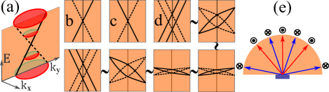
Figure 1: (a) Band dispersion of a Dirac fermion. The glide-invariant cross-section of a Dirac cone corresponds to a right- and left-moving mode, as indicated by two intersecting black lines. A solid (resp. dashed) line corresponds to the glide eigenvalue being $\Delta_{+}$ (resp. $\Delta_{-}$). (b-d) Glide-invariant cross sections of a variety of surface states. (e) A glide-invariant Bloch state (localized to the rectangular sample) absorbs a photon and is emitted as a superposition of plane waves travelling in several directions, as illustrated by the fan of arrows parallel to the glide-invariant plane (colored orange); for blue arrows, the photoelectron spin points into the board, and for red it points out.

One of our aims is to extend this classification to describe glide-symmetric solids – inclusive of insulators and topological metals – and to further elucidate the smoking-gun experimental signature of each class of solids. As described in Sec. II, the classification of topological solids is $\mathbb{Z}_{4}{\oplus}\mathbb{Z}$, with $\mathbb{Z}$ corresponding to the net number of Weyl points in a symmetry-reduced quadrant of the Brillouin zone. Each class of $\mathbb{Z}_{4}{\oplus}\mathbb{Z}$ can be experimentally distinguished through (a) the holonomy of bulk Bloch functions over noncontractible loops of the Brillouin torus, as well as through (b) the photoemission spectroscopyCardona and Ley (1978); Hufner (2003) (PES) of surface states, as discussed in Sec. IV. (a) and (b) are related by the bulk-boundary correspondenceFidkowski et al. (2011); Huang and Arovas (2012); Alexandradinata et al. (2016) of topological insulators and metals.

We propose that our theory is materialized in Sec. III by Ba₂Pb, uniaxially-stressed Na₃Bi, and KHgSb; they respectively fall into the classes: ($\chi^{+}{\in}\mathbb{Z}_{4},{\cal C}{\in}\mathbb{Z}){=}(3,0$), ($1,0$), and ($2,0$). For the Dirac semimetal Na₃Bi, we consider a stress that preserves the glide symmetry but destabilizes the Dirac crossings between conduction and valence bands,Wang et al. (2012) thus inducing a transition from a Dirac semimetal (with space group $D_{6h}^{4}$) to a $\chi^{+}{=}1$ topological insulator (with nonsymmorphic space group 63); such a transition is deducible using the methods of Topological Quantum Chemistry.Bradlyn et al. (2017) While it is known that Ba₂Pb and gapped Na₃Bi belong to the same nontrivial phase under the $\mathbb{Z}_{2}$ time-reversal-symmetric classification,Wang et al. (2012); Sun et al. (2011) here we propose that they are distinct phases in the $\mathbb{Z}_{4}$ glide-symmetric classification, and may be distinguished by photoemission spectroscopy.

Measuring the $\mathbb{Z}_{4}$ topological invariant through photoemission relies on identifying the glide eigenvalues ($\Delta_{\pm}$) of Bloch states before they are photo-excited [cf. Fig. 3(c-h)]. By combining angle-resolved PES with dipole selection rules,Gobeli et al. (1964); Hermanson (1977) it is known how to determine the integer-spin representation of glide for solids without spin-orbit coupling.Pescia et al. (1985); Prince (1987) However, this method is insufficient to determine half-integer-spin representations of glide for spin-orbit-coupled solids, which are the subject of this work. Here, we show that spin- and angle-resolved PES, which was not addressed during the previous works,Gobeli et al. (1964); Hermanson (1977); Pescia et al. (1985); Prince (1987); Borstel et al. (1981) provides the missing ingredient to identify glide eigenvalues – and therefore the $\mathbb{Z}_{4}$ index – in spin-orbit-coupled solids.

Our proposed method relies on photoexciting a glide-invariant Bloch state with linearly-polarized radiation. The excited photoelectron is emitted (into vacuum) as a quantum superposition of plane waves, with wavevectors differing only by reciprocal vectors of the solid (with a surface). The wavevectors lying within the glide-invariant plane form a fan of rays that is illustrated in Fig. 1(e). If the polarization vector of the incoming radiation lies orthogonal to the glide-invariant plane, then photoelectrons on any pair of adjacent rays are fully spin polarized in opposite directions – normal and antinormal to the glide-invariant plane. As we will demonstrate in Sec. V, this perfect spin-momentum locking of the photoelectron is a general manifestation of spin-orbit coupling in all glide-symmetric solids (trivial or topological, insulating or metallic); the generalization to mirror-symmetric solids will also be discussed. As an orthogonal application of this locking, one may generate a fully spin-polarized photoelectronic current (photocurrent, in short) by isolating one of the rays in Fig. 1(e) using standard angle-resolved PES techniques. The potential applications to solid-state spectroscopy are discussed in Sec. LABEL:sec:discussion.

The reader who is solely interested in this spin-momentum locking (and how it is utilized to resolve glide eigenvalues in PES) may jump straight to Sec. V, which has been designed to be a self-contained exposition. In Sec. LABEL:sec:discussion, we elaborate on our proposal to generate spin-polarized photocurrents, as well as compare it with existing theoretical proposals. We also summarize our main results, and discuss further experimental implications.

I Preliminaries on nonsymmorphic space-group representations

Throughout this work, we focus on spin-orbit-coupled solids whose space groups contain (minimally) the operations of time reversal and glide. We adopt a Cartesian coordinate system $(x,y,z)$, with corresponding unit directional vectors $(\vec{\boldsymbol{x}},\vec{\boldsymbol{y}},\vec{\boldsymbol{z}})$, such that the glide symmetry (denoted as $g_{x}$) maps $(x,y,z){\to}({-}x,y{+}R_{2}/2,z)$, where $R_{2}$ is the lattice period in the $\vec{\boldsymbol{y}}$ direction. That is, $g_{x}$ is the composition of two commuting operations: a reflection ($r_{x}$) that inverts $x$, and a translation by half a lattice period in $\vec{\boldsymbol{y}}$. This implies $g_{x}^{2}$ is the product of a full lattice translation and $r_{x}^{2}$; the latter acts on spinor wavefunctions like a $2\pi$ rotation, i.e., it produces a ${-}1$ phase factor.

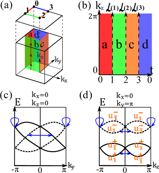
Figure 2: (a) 3D Brillouin zone (BZ) of glide-symmetric solids. For certain nonsymmorphic space groups which contain glide symmetry (e.g., $D_{6h}^{4}$, the space group of KHgSb), their BZs are not cubic, and figure (a) should be understood as a modified BZ corresponding to a non-primitive real-space unit cell; further details may be found in App. C. We will define topological invariants on a 2D subregion that combines four colored faces, which are labelled $abcd$ and parametrized in (b). Red ($a$) and orange ($c$) faces are glide-invariant. (c-d) For noncentrosymmetric space groups, we illustrate typical energy-band dispersions on two glide- and time-reversal-invariant lines, the first at fixed $k_{x}{=}k_{z}{=}0$, and the second at fixed $k_{x}{=}0,k_{y}{=}\pi$ ($R_{2}{=}1$). Solid and dashed lines respectively indicate bands in the $\Delta_{+}$ and $\Delta_{-}$ representations, with corresponding glide eigenvalues $\Delta_{\pm}(k_{y}){=}{\pm}i\exp[{-}ik_{y}/2]$. Arrows indicate states related by time reversal.

Let us review the irreducible half-integer-spin representations of glide and discrete translational symmetries. The irreducible representations of translations are Bloch states labelled by a crystal wavevector $\boldsymbol{k}{=}(k_{x},k_{y},k_{z})$ in the first Brillouin zone (BZ). Since $g_{x}$ maps $\boldsymbol{k}{\to}({-}k_{x},k_{y},k_{z})$, the glide-invariant Bloch functions lie in two cuts of the BZ: the $k_{x}{=}0$ cut through the BZ center will be referred to as the central glide plane, and the $k_{x}{=}\pi/a_{1}$ plane (with $2\pi/a_{1}$ a reciprocal period in the $\vec{\boldsymbol{x}}$ direction) will be referred to as the off-center glide plane. As illustrated in Fig. 2(a), the positive-$k_{y}$ halves of the central and off-center glide plane are labelled by $c$ and $a$ respectively.

Let $\hat{g}_{x}$ be an operator representing $g_{x}$ on spinor wavefunctions. The action of $\hat{g}_{x}^{2}$ on a glide-invariant spinor Bloch function produces a phase ${-}e^{{-}ik_{y}R_{2}}$, hence the possible eigenvalues of $\hat{g}_{x}$ fall into two branches of $\Delta_{\pm}(k_{y}){:}{=}{\pm}i\exp[-ik_{y}R_{2}/2]$. A Bloch state with glide eigenvalue $\Delta_{\pm}(k_{y})$ is said to be in the $\Delta_{\pm}(k_{y})$ representation; we will use ‘eigenvalue’ and ‘representation’ interchangeably. The typical energy band dispersions along two glide- and time-reversal-invariant lines are illustrated in Fig. 2(c-d); each solid black line (resp. dashed black line) indicates a band in the $\Delta_{+}$ (resp. $\Delta_{-}$) representation; this convention is adopted in all figures. The symmetry-enforced band connectivities in Fig. 2(c-d) are further explained in App. A.2.

II Classification of nonsymmorphic topological solids

II.1 Zak-phase expression of the $\mathbb{Z}_{4}$ invariant

In Ref. Shiozaki et al., 2016, a topological invariant $\chi^{+}{\in}\mathbb{Z}_{4}{:}{=}\{0,1,2,3\}$ – expressible as an integral of the Berry connection and curvature – was introduced to classify glide-invariant topological insulators. The same invariant provides a partial classification of glide-invariant topological (semi)metals, so long as touchings – between conduction and valence bands – occur away from the bent, 2D subregion colored in Fig. 2(a). This subregion resembles the face of a rectangular pipe (with its ends identified due to the periodicity of the BZ). The faces of the cylinder are denoted $a,b,c$ and $d$, with $c$ and $a$ belonging to the central and off-center glide planes respectively. In the absence of additional point-group symmetry that might restrict conduction-valence touchings to $abcd$,Fang et al. (2012) we may assume in the generic situation that such touchings occur elsewhere.

Let us present an equivalent reformulation of the $\mathbb{Z}_{4}$-invariant ($\chi^{+}$) through the matrix holonomy of multi-band Bloch functions over the Brillouin torus. The comparative advantages of our formulation are that the eigenvalues of the holonomy matrix, as represented by the graphs in Fig. 3: (i) are potentially measurable by interference experiments,Atala (2013); Li et al. (2015) (ii) are directly relatable to surface states through the bulk-boundary correspondence,Fidkowski et al. (2011); Huang and Arovas (2012); Alexandradinata et al. (2016) as will be elaborated below, and (iii) are efficiently computed from tight-binding models and first-principles calculations.Soluyanov and Vanderbilt (2011a); Yu et al. (2011); Alexandradinata et al. (2014a) In this section, we will explain how the aforementioned graphs are attained, and describe an elementary method to identify $\chi^{+}$ from these graphs. The proof of equivalence between our holonomy-formulation of $\chi^{+}$ and the Shiozaki-Sato-Gomi formulation is postponed to App. B.

To begin, let us consider the parallel transport of Bloch states in the z-direction, i.e., the wavenumber $k_{z}$ of a Bloch state is advanced by a reciprocal period, while the reduced wavevector $\boldsymbol{k}_{\parallel}{=}(k_{x},k_{y})$ is fixed. We consider a family of noncontractible loops within $abcd$ [Fig. 2(a)]; this family is parameterized by $t{\in}[0,4]$ with $4{\equiv}0$ [Fig. 2(b)]. A Bloch state that is parallel-transported over a loop does not necessarily return to its initial state; the mismatch between initial and final states is represented by a holonomy matrix ${\cal W}$ in the space of occupied bands (numbering $n_{\scriptscriptstyle{{occ}}}$). ${\cal W}$ is known as the Wilson loop of the non-abelian Berry gauge field,Wilczek and Zee (1984) and its unimodular eigenvalues $\{\exp[i\theta_{j}(t)]|j{=}1,2,\ldots,n_{\scriptscriptstyle{{occ}}};t{\in}[0,4]\}$ are the Zak phase factors. In analogy with energy bands, we may refer to $\theta_{j}(t)$ as the dispersion of a ‘Zak band’ with band index $j$. For $t{\in}[0,1]$ and $[2,3]$ (which correspond to the glide-invariant faces $a$ and $c$), ${\cal W}$ block-diagonalizes into two $n_{\scriptscriptstyle{{occ}}}/2$-by-$n_{\scriptscriptstyle{{occ}}}/2$ blocks,Höller and Alexandradinata (2018) corresponding to the two representations ($\Delta_{\pm}$) of glide; we may therefore label the Zak bands as $\{\theta_{j}^{\pm}\}_{\scriptscriptstyle{j{=}1}}^{\scriptscriptstyle{n_{\scriptscriptstyle{{occ}}}/2}}$.

The $\mathbb{Z}_{4}$ topological invariant is expressible as:

For this expression to be well-defined modulo four, we choose that (i) $\theta_{j}$ is smooth with respect to $t$ over $[1,2]$, (ii) $\theta_{j}^{\pm}$ is smooth over $[0,1]$ and $[2,3]$, and (iii) $\theta_{j}^{\pm}(t)$ are pairwise degenerate at $t{=}0$ and $3$. To clarify (iii), for any $j\in\{1,\ldots,n_{\scriptscriptstyle{{occ}}}/2\}$, there exists $j^{\prime}\in\{1,\ldots,n_{\scriptscriptstyle{{occ}}}/2\}$ such that $j\neq j^{\prime}$, $\theta_{j}^{\pm}(0)=\theta_{j^{\prime}}^{\pm}(0)$, and $\theta_{j}^{\pm}(3)=\theta_{j^{\prime}}^{\pm}(3)$.

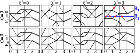
Figure 3: Classification of glide-symmetric insulators by a strong $\mathbb{Z}_{4}$ invariant ($\chi^{+}$) and a weak $\mathbb{Z}_{2}$ invariant (${\cal P}_{01}$). The vertical axis has the double interpretation as a Berry-Zak phase $\theta{\in}[0,2\pi]$, or as the energy of a surface-localized state (that interpolates between conduction and valence bands). Bands are doubly-degenerate along 30, and glide-invariant along 01 and 23 only.

From Eq. (LABEL:wilsonex), we derive the simplest way to identify $\chi^{\pm}$ from the Zak-phase spectrum: for an arbitrarily chosen $\bar{\theta}$, draw a constant-$\bar{\theta}$ reference line (as illustrated in blue in the right-most column of Fig. 3) and consider its intersections with Zak bands (indicated by red dots). For each intersection occurring at $t{\in}(1,2)$, we calculate the sign of the velocity $d\theta/dt$, and sum this quantity over all intersections [over $t{\in}(1,2)$] to obtain ${\cal S}_{12}(\bar{\theta})$; for $t{\in}[0,1]$ and $[2,3]$, we consider only intersections with Zak bands in the $\Delta_{\pm}$ representation, and we similary sum over sgn[$d\theta/dt$] to obtain ${\cal S}^{\pm}_{01}(\bar{\theta})$ and ${\cal S}^{\pm}_{23}(\bar{\theta})$ respectively. The following weighted sum of ${\cal S}^{\pm}_{ij}$ and ${\cal S}_{12}$,

$${{\cal S}^{\pm}(\bar{\theta})=2{\cal S}^{\pm}_{01}(\bar{\theta})+{\cal S}_{12}(\bar{\theta})+2{\cal S}^{\pm}_{23}(\bar{\theta}),}$$ (1)

satisfies that $({\cal S}^{\pm}(\bar{\theta}_{1}){-}{\cal S}^{\pm}(\bar{\theta_{2}}))/4{\in}\mathbb{Z}$ for any two reference lines at constant $\bar{\theta}_{1}$ and $\bar{\theta}_{2}$, e.g., compare ${\cal S}^{+}(\bar{\theta}_{1}){=}2(0){+}1{+}2({-}1){=}{-}1$ [upper blue line in Fig. 3] with ${\cal S}^{+}(\bar{\theta}_{2}){=}2({+}1){+}1{+}2(0){=}3$ [lower blue line]. Equivalently stated, if we henceforth view ${\cal S}^{\pm}(\bar{\theta})$ as an element in $\mathbb{Z}_{4}$, then this quantity becomes independent of $\bar{\theta}$. By also viewing $\chi^{\pm}$ as a $\mathbb{Z}_{4}$ quantity, we may identify ${\cal S}^{\pm}{\equiv}\chi^{\pm}$ by comparing Eq. (LABEL:wilsonex) with Eq. (1). To clarify, $\equiv$ denotes an identity between two equivalence classes in $\mathbb{Z}_{4}$.

II.2 Extended classification of glide-symmetric topological solids

We now demonstrate that $\chi^{+}{\equiv}{-}\chi^{-}$ for insulators, while this is not necessarily true for Weyl metals. We are considering time-reversal- and glide-symmetric Weyl metals that occur only in non-centrosymmetric space groups.Wan et al. (2011); Halasz and Balents (2012) Such metals may be characterized by counting the net number of Weyl nodes in the open Brillouin-zone quadrant ${\cal O}$ surrounded by (but not including) the faces $abcd$ [Fig. 3(a)]. ${\cal O}$ resembles the interior of a rectangular pipe, and its properties determine those of the other three quadrants owing to $g_{x}$ and time-reversal symmetry. Each Weyl node has a signed charge ($q$) corresponding to whether it is a source ($q{=}{+}1$) or sink ($q{=}{-}1$) of the Berry field strength; the net charge within ${\cal O}$ is quantified by the bent Chern number (${\cal C}$),Alexandradinata et al. (2014b) which may be formulated as the net winding of $\theta(t)$ for $t{\in}[0,4]$, or equivalently as the summation of sign[$d\theta/dt$], over all intersections with a constant-$\bar{\theta}$ reference line. The sum is carried out over all bands indiscriminate of their symmetry representations, therefore

$${{\cal C}=\tfrac{1}{2}\big{[}\;{\cal S}^{+}(\bar{\theta})+{\cal S}^{-}(\bar{\theta})\;\big{]}+{\cal S}_{30}(\bar{\theta}).}$$ (2)

To clarify, ${\cal S}_{30}$ here is the summation of sign[$d\theta/dt$] over the interval $t\in(3,4)$, which corresponds to the blue line $30$ in Fig. 2(a); ${\cal S}_{30}$ must be even because Zak bands are doubly-degenerate due to $g_{x}T$ symmetry.Wang et al. (2016) While each of ${\cal S}^{\pm}$ and ${\cal S}_{30}$ may individually depend on the choice of reference line, their weighted sum (${\cal C}$) does not. Applying that $2S_{30}$ is an integer multiple of four, and the relation ${\cal S}^{\pm}{\equiv}\chi^{\pm}$ from the previous paragraph, we derive

$${(\chi^{+}+\chi^{-})\equiv 2{\cal C}\;\bmod\;4,}$$ (3)

which implies a $\mathbb{Z}{\oplus}\mathbb{Z}_{4}$ classification of glide-symmetric solids, inclusive of metals and insulators. To recapitulate, $\mathbb{Z}$ counts the net number of Weyl points in a symmetry-reduced quadrant of the BZ. Representative examples for ${\cal C}{=}1$ and $2$ are illustrated in Fig. 4.

Figure 4: Topological classification of glide-symmetric metals with ${\cal C}{\in}\mathbb{Z}$ and $\chi^{+}{\in}\mathbb{Z}_{4}$. A finer classification is possible with the introduction of ${\cal P}_{01}{\in}\mathbb{Z}_{2}$ – a weak topological invariant that is defined in Sec. III. Note that $\chi^{+}{\in}\{0,1,2,3\}$ should be viewed as the mod-four equivalence class of the quantity defined in Eq. (LABEL:wilsonex), or equivalently in Eq. (1).

II.3 Surface states of nonsymmmorphic topological solids

We now extend our discussion to the physics of surface states. We terminate the solid in the z-direction by introducing a surface that is symmetric under glide and discrete translations in the xy plane. We further assume that the surface is clean and does not undergo a symmetry-breaking reconstruction. So long as the above-stated symmetries are preserved, the exact termination of the surface (including relaxation effects) is not essential to our discussion – we are concerned only with topological aspects of the surface states.

The translational symmetry implies the existence of a surface Brillouin zone ($sBZ$) that is parametrized by the wavevector $\boldsymbol{k}_{\parallel}$; recall that $(\boldsymbol{k}_{\parallel},k_{z})$ parametrizes the bulk Brillouin zone ($bBZ$) of a solid that is periodic in three directions. Energy bands whose wavefunction is localized to the surface shall be referred to as surface bands. Such surface bands can only exist at $\boldsymbol{k}_{\parallel}{\in}sBZ$ for which there is a bulk energy gap at the reduced wavevector $\boldsymbol{k}_{\parallel}$; in particular, they cannot exist at $\boldsymbol{k}_{\parallel}{\in}sBZ$ if a Weyl point lies at $(\boldsymbol{k}_{\parallel},k_{z}){\in}bBZ$ for some $k_{z}$.

Our previous discussion of Zak bands may be related to surface bands by the bulk-boundary correspondence. This correspondence states that the connectivity of Zak bands (over the reduced wavevector $\boldsymbol{k}_{\parallel}$) is topologically equivalent to the connectivity of surface bands (over the surface wavevector $\boldsymbol{k}_{\parallel}$).Fidkowski et al. (2011); Huang and Arovas (2012); Alexandradinata et al. (2016) We shall only concern ourselves with the connectivity over on the high-symmetry lines $01$, $12$, $23$, $30$ in $sBZ$ [see Fig. 3(a)]; they are respectively the projections of the faces $a$, $b$, $c$ and $d$ in $bBZ$. Given our assumption that Weyl points (if they exist) lie away from $abcd$, surface bands potentially exist along $01230$, and their connectivity is then well-defined.

$\chi^{\pm}$ may be identified by considering intersections between surface bands (over $0123$) and a constant-energy reference line (e.g., the Fermi level). This reference line is chosen so as not to intersect any bulk bands; ${\cal S}_{12}$ and ${\cal S}_{ij}^{\pm}$ in Eq. (1) are defined analogously with the velocities ($d\varepsilon/dt$) of surface bands, instead of Zak bands. We are now ready to justify our heuristic argument for the $\mathbb{Z}_{4}$ classification of glide-symmetric insulators, as formulated in the introductory paragraph: suppose our reference Fermi level lies above the Dirac node, each positive-chirality Dirac surface band (centered at $\boldsymbol{k}_{\parallel}(2){=}\Gamma$) singly intersects the reference line at each of $12$ and $23$; each therefore contributes to $\chi^{+}$ the quantity $2(0){+}({-}1){+}2(1)$; we may therefore interpret the deformation in Fig. 1(d) as the equivalence: $\chi^{+}{=}2{\equiv}{-}2$.

III Materialization of nonsymmorphic topological insulators

In this section, we identify three insulating materials which realize all three nontrivial phases in the $\mathbb{Z}_{4}$ classification given by $\chi^{+}{\equiv}{-}\chi^{-}$. This classification is characterized as strong, in the sense that any nontrivial phase (with $\chi^{+}{\neq}0$ mod 4) cannot be realized by layering lower-dimensional glide-symmetric topological insulators.

As is known from topological K theory,Shiozaki et al. (2016) the full classification of glide-symmetric surface bands is $\mathbb{Z}_{4}{\oplus}\mathbb{Z}_{2}$, where the additional $\mathbb{Z}_{2}$ summand corresponds to a weak classification by a Kane-MeleC. L. Kane and E. J. Mele (2005) invariant (denoted ${\cal P}_{01}{\in}\{0,1\}$) defined over the time-reversal- and glide-invariant plane containing the face $a$. ${\cal P}_{01}$ may be determined by the connectivity of Zak/surface bands on the off-center glide line 01: ${\cal P}_{01}{=}0$ corresponds to a gapped, hourglass-type connectivity along $t{\in}[0,1]$ in the top row of Fig. 3, and ${\cal P}_{01}{=}1$ to a zigzag (quantum-spin-Hall) connectivityRoy (2009b); Fu and Kane (2006) in the bottom row.

Having described in Fig. 3 the connectivity in each nontrivial class of $\mathbb{Z}_{4}{\oplus}\mathbb{Z}_{2}$, we are ready to identify Ba₂Pb, KHgSb, and uniaxially-stressed Na₃Bi as corresponding to $(\chi^{+},{\cal P}_{01}){=}(3,0),(2,0),(1,0),$ from their ab-initio-derived Zak-band connectivity in Fig. 5(a-c).

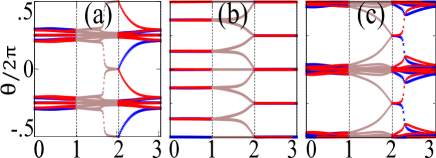
Figure 5: Ab-initio-derived Zak phases of: (a) Ba₂Pb, (b) KHgSb, and (c) uniaxially-stressed Na₃Bi. Along the glide-invariant lines $01$ and $23$, we decompose the Zak phases according to their glide representations: $\Delta_{+}$ is indicated by red circles, and $\Delta_{-}$ by blue.

The parity of $\chi^{+}$ being even (resp. odd) is in one-to-one correspondenceXiong and Alexandradinata (2018) with the trivial (resp. nontrivial) phase in the time-reversal-symmetric, strong $\mathbb{Z}_{2}$ classification. We thus deduce that Ba₂Pb and uniaxially-stressed Na₃Bi belong to the same phase in the time-reversal-symmetric classification (as was derived by other means in previous worksWang et al. (2012); Sun et al. (2011) ), but belong to distinct $\mathbb{Z}_{4}$ phases in the presence of glide symmetry (a novel conclusion of this work). This conclusion is further supported by our analysis of both compounds based on their elementary band representationsZak (1981); Evarestov and Smirnov (1984); Bacry (1993); Bradlyn et al. (2017); Höller and Alexandradinata (2018); Alexandradinata and Höller (2018) – a perspective we develop in App. D.

In comparison, KHgSb is trivial in the time-reversal-symmetric $\mathbb{Z}_{2}$ classification but nontrivial in the glide-symmetric $\mathbb{Z}_{4}$ classification; additional crystalline symmetries (beyond glide) in the space group ($D_{6h}^{4}$) of KHgSb are known to lead to an even finer classification.Alexandradinata et al. (2016) It was argued in Ref. Shiozaki et al., 2016 that KHgSb should belong to the $\chi^{+}{=}2$ class based on the connectivity of its surface states; Fig. 5(b) provides the first evidence based on an explicit calculation of the bulk topological invariant. We remark that a recent polarized Raman scattering studyChen et al. (2017) suggests of a low-temperature lattice instability in KHgSb; such an instability would not break glide symmetry, and we expect that $\chi^{+}{=}2$ should remain valid.

In App. D, we detail the space groups and elementary band representations of these materials, and further describe the stress that should be applied to Na₃Bi – so that it becomes a topological insulator.

IV Photoemission spectroscopy of $\mathbb{Z}_{4}$ invariant

Let us describe how the $\mathbb{Z}_{4}$ invariant [cf. Eq. (1)] is measurable from PES. The velocities ($d\varepsilon/dt$) of surface states are measurable from angle-resolved PES using standard techniques.Cardona and Ley (1978); Hufner (2003) The counting of ${\cal S}^{\pm}_{23}$ (resp. ${\cal S}^{\pm}_{01}$) further requires that we identify the glide representation ($\Delta_{\pm}$) of the pre-excited Bloch state on the glide line intersecting the surface-BZ center (resp. lying on the surface-BZ edge). We propose a spectroscopic method for identifying $\Delta_{\pm}$ on the central glide line 23 ($k_{x}{=}0$) in the next section [Sec. V].

This method cannot be applied to determine $\Delta_{\pm}$ for the off-center glide line $01$, as explained at the end of Sec. V. However, we may anyway determine the $\mathbb{Z}_{4}$ invariant for materials with no Fermi-level surface states along $01$, in which case ${\cal S}^{\pm}_{01}{=}0$. Indeed, there is no topological reason to expect surface states along $01$ for materials with a trivial weak index (${\cal P}_{01}{=}0$), as explained in Sec. III. Our calculations show that all three materials (proposed in Sec. III) have ${\cal P}_{01}{=}0$, and have no Fermi-level surface states along $01$ for a perfect surface termination (i.e., ignoring surface relaxation or reconstruction). We remark that ${\cal P}_{01}{=}0$ is guaranteed for certain space groups (including those of KHgSb and uniaxially-stressed Na₃Bi), owing to a symmetry of a discrete translation (in a direction oblique to the surface); this is elaborated in App. C.

Let us address one final subtlety about the identification of $\chi^{\pm}$ (or ${\cal C}$) from photoemission. $\chi^{\pm}$ and ${\cal C}$ have been defined with respect to a fixed, Cartesian, right-handed coordinate system parametrized by $(k_{x},k_{y},k_{z})$. A spectroscopist who examines a solid necessarily has to pick a coordinate system and measure the topological invariants with respect to this choice. Will two measurements of $\chi^{\pm}$ – of the same solid but based on different coordinates chosen by the spectroscopist – unambiguously agree?

The glide symmetry may be exploited to reduce this coordinate ambiguity: we may always choose a right-handed, Cartesian coordinate system where $\vec{\boldsymbol{x}}$ (resp. $\vec{\boldsymbol{y}}$) lies parallel to the reflection (resp. fractional translational) component of the glide, i.e., the glide maps $(x,y,z)\rightarrow(-x,y\pm R_{2}/2,z)$; from the experimental perspective, this presupposes some knowledge about the crystallographic orientation of a sample, as discussed further in App. LABEL:app:lightsource. This prescription does not uniquely fix the coordinate system: supposing $(x,y,z)$ satisfies the above condition, so would $(x^{\prime},y^{\prime},z^{\prime})=(-x,-y,z)$, and more generally any coordinate system that is related to $(x,y,z)$ by two-fold rotations about $\vec{\boldsymbol{x}},\vec{\boldsymbol{y}}$ or $\vec{\boldsymbol{z}}$; such rotations, denoted as $p\in\{C_{2x},C_{2y},C_{2z}\}$ respectively, preserve the orientation (or handedness) of the coordinate system.

It follows from the above discussion that two spectroscopists, given an identical sample, may set down different coordinate systems parametrized by $(x,y,z)$ and $(x^{\prime},y^{\prime},z^{\prime})=p\circ(x,y,z)$ respectively; $p$ need not be a symmetry of the solid. Following identically the instructions of this work, the two spectroscopist would determine the $\mathbb{Z}_{4}$ and $\mathbb{Z}$ invariants based on their chosen coordinates; suppose the first spectroscopist measures the numbers $(\chi^{\pm},{\cal C})$, and the second measures $(p\circ\chi^{\pm},p\circ{\cal C})$. As proven in App. E, for $p{\in}\{C_{2x},C_{2y}\}$, $p{\circ}\chi^{\pm}{=}{-}\chi^{\mp}$ and $p{\circ}{\cal C}{=}{-}{\cal C}$. On the other hand, $C_{2z}{\circ}\chi^{\pm}{=}\chi^{\pm}$ and $C_{2z}{\circ}{\cal C}{=}{\cal C}$. In all cases, Eq. (3) is invariant. We may then draw the following conclusions depending on whether ${\cal C}$ is even or odd: if even (which includes the insulating case), then $\chi^{\pm}{\equiv}{-}\chi^{\mp}$ according to Eq. (3), and two right-handed (or two left-handed) spectroscopists always agree on their measured values for $\chi^{\pm}$. That is to say, $\chi^{\pm}=p\circ\chi^{\pm}$ for $p{\in}\{C_{2x},C_{2y},C_{2z}\}$. If, however, ${\cal C}$ is odd, two right-handed spectroscopists are only guaranteed to agree on the parity of $\chi^{\pm}$. Despite this ambiguity, once a convention for a coordinate system is fixed, the distinction between phases is well-defined.

V Glide-resolved photoemission spectroscopy

This section is a self-contained exposition on a spectroscopic method to identify the glide representation $\Delta_{\pm}(k_{y})$ of initial Bloch states (i.e., Bloch states before photo-excitation). We assume only that the reader is familiar with basic notions in the representation theory of space groups, as reviewed briefly in Sec. I.

Our method is applicable to surface or bulk photoemission. That is to say, our initial Bloch states may be localized to the surface (on which the radiation is incident) or delocalized throughout the bulk of the solid. In both cases, we focus on initial Bloch states with wavevectors on the glide-invariant line intersecting the surface-BZ center (the central glide line), as indicated by 23 in Fig. 2(a). Adopting our choice coordinates for real and quasimomentum spaces, this glide-invariant line lies at $k_{x}{=}0$, for a glide operation $g_{x}$ that maps $(x,y){\rightarrow}({-}x,y{+}R_{2}/2)$, with $R_{2}$ a primitive surface-lattice period.

We will first describe the basic idea in simple, intuitive terms in Sec. V.1, where we specialize to normally incident, linearly polarized and monochromatic light. We shall assume that the radiation gauge and dipole approximation are applicable to the electron-photon coupling; the dipole approximation is relaxed in the formal theory presented in Sec. V.2, where we also generalize to other incident angles and polarizations.

V.1 Basic principle

Suppose an electron – with Bloch wave function $\psi_{i}$, initial energy $\varepsilon_{i}$, and wavevector $\boldsymbol{k}_{\parallel}{=}(0,k_{y})$ – absorbs a photon and is excited to a photoelectronic state with energy $\varepsilon_{p}$. The electron-photon coupling is proportional to $\boldsymbol{a}{\cdot}\hat{\boldsymbol{p}}$ in the radiation gauge, where $\boldsymbol{a}{\propto}\vec{\epsilon}$ is the divergence-free electromagnetic vector potential, and the electromagnetic scalar potential is chosen to vanish. $\hat{\boldsymbol{p}}$ above is the electronic momentum operator, which should be distinguished from the crystal wavevector $\boldsymbol{k}$. We choose normally-incident, linearly-polarized radiation with the polarization vector $\vec{\epsilon}$ lying parallel to the glide plane; for the $g_{x}$-invariant yz-plane, $\vec{\epsilon}{=}\vec{\boldsymbol{y}}$ is the unit vector in the y-direction [cf. Fig. 6(c)]. In the dipole approximation, $\boldsymbol{a}{\cdot}\hat{\boldsymbol{p}}$ reduces to a spatially-homogeneous constant multiplied with $\hat{p}_{y}$. Since $\hat{p}_{y}$ is invariant under $g_{x}$ and surface-parallel translations, $\psi_{i}$ and the emitted photoelectron belong to the same representation of these symmetries; we shall refer to this constraint as a selection rule.

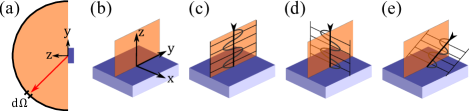
Figure 6: (a) Photoemission setup: a sample (colored blue) is radiated and emits photoelectrons which are collected in a hemispherical cup. (b) Our choice coordinate system. (c-e) illustrate our favored incidence angles and polarizations. The spatial variation and directional vector of the electric field are indicated by the sinuisoidal lines.

This selection rule has observable consequences for a photoelectron that is measured at the detector. This photoelectron generically has a complicated wavefunction with a component in vacuum that extends toward the detector, and a separate component that penetrates the solid up to an escape depth.Mahan (1970) Consider how a photoelectron transforms under any spacetime symmetry of a surface-terminated solid (in short, surface-preserving symmetry), as exemplified in this context by $g_{x}$ and surface-parallel translations. Such transformation is completely determined by the transformation of the photoelectron’s component in vacuum, because a surface-preserving isometry never maps a point inside a solid to a point outside. Since vacuum is symmetric under continuous translations and $SU(2)$ spin rotations, the vacuum component is simply a linear combination of plane waves with energy $\varepsilon_{p}{:}{=}(\hbar p)^{2}/2m$ and wavevector $\boldsymbol{p}$ (note $|\boldsymbol{p}|{:}{=}p$); for each $\boldsymbol{p}$, there are two plane waves distinguished by the photoelectron spin. Due to the symmetry of discrete surface-parallel translations, the surface-parallel component of $\boldsymbol{p}$ must equal $\boldsymbol{k}_{\parallel}$ – of the initial Bloch state – modulo a surface-parallel reciprocal vector $\boldsymbol{G}_{\parallel}$; each $\boldsymbol{G}_{\parallel}$ corresponds to a different angle for photoelectrons to come out of the solid, as illustrated by the fan of arrows in Fig. 1(e).

To understand the symmetry representation of the photoelectron, we must therefore analyze the symmetry properties of spin-polarized plane waves. Each $g_{x}$-invariant plane-wave state $\big{|}\phi_{\boldsymbol{p},s}\big{\rangle}$ is a tensor product ($\big{|}\phi_{\boldsymbol{p}}\big{\rangle}{\otimes}\big{|}s\big{\rangle}$) of a spinless plane wave ($\big{\langle}\boldsymbol{r}\big{|}\phi_{\boldsymbol{p}}\big{\rangle}{=}e^{i\boldsymbol{p}\cdot\boldsymbol{r}}$) and a spinor $\big{|}s{=}{\pm}1\big{\rangle}$ in the eigenbasis of $S_{x}$. The momentum $\boldsymbol{p}$ lies parallel to the glide plane ($p_{x}{=}0$), and the spin orthogonal to the glide plane, such that

$${\hat{g}_{x}\big{|}\phi_{\boldsymbol{p},s}\big{\rangle}{=}{-}i\,s\,e^{-ip_{y}R_{2}/2}\big{|}\phi_{\boldsymbol{p},s}\big{\rangle};\;S_{x}\big{|}s\big{\rangle}{=}s\frac{\hbar}{2}\big{|}s\big{\rangle}.}$$ (4)

The phase ${-}i\,s$ originates from reflecting $\big{|}s\big{\rangle}$ in the x-direction; after all, this reflection is just the composition of spatial inversion (which acts trivially on spin) and a two-fold rotation $e^{-i\pi(L_{x}+S_{x})}$ about the x-axis. The phase $e^{-ip_{y}R_{2}/2}$ in Eq. (4) originates from translating $\phi_{\boldsymbol{p}}$ by half a lattice period in the y-direction. We can always express $p_{y}{=}k_{y}{+}2\pi n/R_{2}$ such that $k_{y}$ lies in the first Brillouin zone (BZ) and $n{\in}\mathbb{Z}$. Recalling from Sec. I that a Bloch state in the $\Delta_{\pm}(k_{y})$ representation has glide eigenvalue ${\pm}ie^{-ik_{y}R_{2}/2}$, we conclude that $\phi_{\boldsymbol{p},s}$ transforms in the $\Delta_{-s}(k_{y})$ representation if $n$ is even, and in the $\Delta_{+s}(k_{y})$ representation if $n$ is odd.

Combining this symmetry analysis with our selection rule, we find the following constraint for a photoelectron that is excited from an initial Bloch state ($\boldsymbol{k}_{\parallel}{=}(0,k_{y})$) in the $\Delta_{+}(k_{y})$ representation. Namely, the photoelectronic plane wave ($\big{|}\phi_{\boldsymbol{p},s}\big{\rangle}$) that is detected must also belong in the $\Delta_{+}(k_{y})$ representation; this implies that the spin of the photoelectron is nontrivially locked to its momentum: expressing the surface-parallel component of $\boldsymbol{p}$ as $\boldsymbol{p}_{\parallel}{=}(0,p_{y}{=}k_{y}{+}2\pi n/R_{2})$, then

$$\langle S_{x}\rangle=s\frac{\hbar}{2}=\begin{cases}+\frac{\hbar}{2},&\text{if}\;n\in 2\mathbb{Z}+1\\ -\frac{\hbar}{2},&\text{if}\;n\in 2\mathbb{Z}\end{cases}$$ (5)

If the initial Bloch state were in the $\Delta_{-}$ representation, then Eq. (5) holds with the interchange of ‘odd’ and ‘even’. This spin-momentum locking manifests the glide symmetry of the spin-orbit interaction. As a consequence, each ray of the fan [in Fig. 1(e)], corresponding to a unique value of $n$, is fully spin polarized; nearest-neighbor rays always have opposing polarizations. The angle of each ray is determined by energy conservation:

$${\varepsilon_{i}+\hbar\omega=\frac{\hbar^{2}(k_{y}+2\pi n/R_{2})^{2}+\hbar^{2}p_{z}^{2}}{2m}.}$$ (6)

Tantalizingly, each ray may be isolated experimentally by standard spin- and angular-resolution techniques that measure $\langle S_{x}\rangle$ and $p_{y}$;Hufner (2003) this allows us to spectroscopically identify the glide representation of an initial state.

V.2 One-step theory of glide-resolved photoemission

To justify this spin-momentum locking rigorously, we employ the steady-state scattering formulationLippmann and Schwinger (1950); Gell-Mann and Goldberger (1953); Bethe and Salpeter (1957) of the one-step theoryAdawi (1964); Mahan (1970); Feibelman and Eastman (1974) of photoemission. We begin with the component of the Hamiltonian that describes the solid in the absence of radiation; in the independent-electron approximation, this assumes the standard Pauli form: $H_{e}{=}(\hbar\hat{\boldsymbol{p}})^{2}/2m{+}{V}$, in the non-relativisitic limitFoldy and Wouthuysen (1950); Blount (1962) of the Dirac Hamiltonian; $V$ includes a scalar potential, the spin-orbit coupling, and in principle also the Darwin term. Since $V$ encodes a mean-field interaction of a single electron with other electrons as well as the ionic lattice, $V$ falls off to zero rapidly away from the solid.Ashcroft and Mermin (1976) Here, we have adopted the usual electrostatic convention for the zero of energy – as the energy of a zero-momentum plane wave in free space (far away from the solid).

Suppose $\psi_{i}$, an eigenstate of $H_{e}$ with energy $\varepsilon_{i}$ below the Fermi level, absorbs a single photon with energy $\hbar\omega$; $i$ here includes all quantum numbers of the eigenstate, including the band index and the crystal wavevector. The corresponding photoelectron has energy $\varepsilon_{i}{+}\hbar\omega{>}0$, and a spinor wavefunction of the form:

$${\Psi_{p,i}=G^{\scriptscriptstyle{+}}(\varepsilon_{p})H_{int}\psi_{i},\;\;\;\;\varepsilon_{i}+\hbar\omega:=\varepsilon_{p}:=(\hbar p)^{2}/2m}$$ (7)

to lowest order in the electron charge. Here we have introduced the advanced/retarded Green’s functions: $G^{\scriptscriptstyle{\pm}}(\varepsilon){=}(\varepsilon{-}H_{e}{\pm}i\delta)^{\text{-}1}$, with infinitesimal $\delta{>}0$. The electron-photon coupling has the form $H_{int}{=}|e|(\boldsymbol{a}{\cdot}\hat{\boldsymbol{p}}{+}\hat{\boldsymbol{p}}{\cdot}\boldsymbol{a})/2mc$ in the temporal gauge, where the scalar potential vanishes; $\boldsymbol{a}$ here is the screenedFeibelman and Eastman (1974); Feibelman (1982) electromagnetic vector potential in the solid. The Zeeman interaction with the spin magnetic moment typically has a small effect relative to the $\boldsymbol{a}{\cdot}\hat{\boldsymbol{p}}$ term,Feuchtwang et al. (1978); Feder (2013a) and is therefore neglected from $H_{int}$; a further evaluation of the Zeeman interaction is provided in Sec. LABEL:sec:discussion.

Given that $\psi_{i}$ belongs to a certain glide representation, we would like that the photoelectron transforms in a glide representation that is uniquely determined by the representation of $\psi_{i}$. Such a selection rule exists if the electron-photon coupling $H_{int}$ transforms in a one-dimensional representation of glide symmetry, i.e., $\hat{g}_{x}H_{int}\hat{g}_{x}^{-1}$ equals $H_{int}$ up to a phase, with $\hat{g}_{x}$ the operator that implements glide reflection [cf. Eq. (4)].

As shown in App. LABEL:app:lightsource, the desired transformation of $H_{int}$ exists for a linearly-polarized light source, with wavevector parallel to the glide-invariant yz plane, and with the polarization vector $\vec{\epsilon}$ either orthogonal [see Fig. 6(d-e)] or parallel [Fig. 6(c)] to the glide-invariant plane. In the standard convention, we identify the orthogonal alignment as $s$ polarization, and the parallel alignment as $p$ polarization, though such identifications are not meaningful for normal incidence.

In the case of normal incidence, the Fresnel equations inform us that the light remains linearly polarized (with the same polarization vector $\vec{\epsilon}$) upon transmission into the solid; that is to say, the vector potential $\boldsymbol{a}$ within the solid remains parallel to $\vec{\epsilon}$. In the orthogonal alignment, $H_{int}{\propto}\boldsymbol{a}{\cdot}\hat{\boldsymbol{p}}{\propto}\hat{p}_{x}e^{-i\omega z/c}$ anticommutes with the glide operator $\hat{g}_{x}$; with the parallel alignment, $H_{int}{\propto}\hat{p}_{y}e^{-i\omega z/c}$ commutes with $\hat{g}_{x}$. In the more general case of non-normal incident angles [see Fig. 6(e)], it is shown in App. LABEL:app:lightsource that

$${\hat{g}_{x}H_{int}\hat{g}_{x}^{-1}=\pm e^{-iq_{y}R_{2}/2}H_{int},}$$ (8)

with the plus (resp. minus) sign applying to $p$ (resp. $s$) polarization, and the additional phase factor $e^{-iq_{y}R_{2}/2}$ originating from a half-lattice translation of the photon field (having wavenumber $q_{y}$ within the solid).

Since $\hat{g}_{x}$ commutes with $G^{\scriptscriptstyle{+}}(\varepsilon_{p})$ [cf. Eq. (7)], $\Psi_{p,i}$ and $H_{int}\psi_{i}$ transform in the same representation of $g_{x}$. That is, if $\psi_{i}$ is a Bloch function ($\boldsymbol{k}_{\parallel}{=}(0,k_{y})$) in the $\Delta_{\pm}(k_{y})$ representation, then $\Psi_{p,i}$ belongs in the $\Delta_{\mp}(k_{y}+q_{y})$ [resp. $\Delta_{\pm}(k_{y}+q_{y})$] representation for $\vec{\epsilon}$ orthogonal (resp. parallel) to the glide-invariant plane; the addition of $q_{y}$ in the argument represents the absorption of the photon’s momentum [cf. Eq. (8)]. Assuming the surface is clean and unreconstructed, $\Psi_{p,i}$ also transforms under discrete translations in the representation $\boldsymbol{k}_{\parallel}{=}(0,k_{y}+q_{y})$.

Let us translate these selection rules to a spin-momentum-locking constraint on the measured photocurrent. We begin with an identity relating $G^{\scriptscriptstyle{\pm}}$ to the free-space Green’s function $G_{0}^{\scriptscriptstyle{\pm}}$:

$${G^{\scriptscriptstyle{\pm}}=G_{0}^{\scriptscriptstyle{\pm}}+G_{0}^{\scriptscriptstyle{\pm}}VG^{\scriptscriptstyle{\pm}};\;G_{0}^{\scriptscriptstyle{\pm}}(\varepsilon):=\big{(}\varepsilon-\tfrac{(\hbar\hat{\boldsymbol{p}})^{2}}{2m}\pm i\delta\big{)}^{\text{-}1}.}$$ (9)

The asymptotic, spherical-wave form of $G_{0}^{\scriptscriptstyle{\pm}}$ is well-known:Griffiths (2005) for $r({:}{=}|\boldsymbol{r}|)$ and

$${r\gg r^{\prime},\;\big{\langle}\boldsymbol{r},s\big{|}G_{0}^{\scriptscriptstyle{\pm}}(\varepsilon_{p})\big{|}\boldsymbol{r}^{\prime},s^{\prime}\big{\rangle}\sim{-}\frac{m}{\hbar^{2}}\frac{e^{\pm ipr}}{2\pi r}e^{\mp i\boldsymbol{p}\cdot\boldsymbol{r}^{\prime}}{\delta_{ss^{\prime}}},}$$ (10)

where $\vec{\boldsymbol{r}}$ is the unit vector parallel to $\boldsymbol{r}$, $\boldsymbol{p}{:}{=}p\vec{\boldsymbol{r}}{:}{=}(p_{x},p_{y},p_{z})$, $\big{|}\boldsymbol{r},s\big{\rangle}$ is an eigenstate of position and $S_{x}$ operators, and $\sim$ denotes the leading asymptotic form for large $r$.

Let us apply the identity Eq. (9) and the asymptotic form of $G_{0}^{\scriptscriptstyle{+}}$ [Eq. (10)] to evaluate $\Psi_{p,i}$ defined in Eq. (7). Combining Eqs. (7)-(9), we derive

Appendix

The appendices are organized as follows:

(A) We briefly review symmetries in the tight-binding method and establish notation that would be used throughout the appendix.

(B) We show the equivalence between the $\mathbb{Z}_{4}$ invariant defined by Shiozaki-Sato-Gomi,Shiozaki et al. (2016) and the Zak-phase expression in Eq. (LABEL:wilsonex).

(D) We detail the space groups and elementary band representations of Ba₂Pb, stressed Na₃Bi, and KHgSb, so as to provide a complementary perspective on their topological nontriviality.

(C) We introduce two symmetry classes of solids with glide symmetry; the two classes are distinguished by the representation of glide symmetry in the 3D Brillouin zone (BZ). In one of the two classes, the weak $\mathbb{Z}_{2}$ invariant is trivial, and a non-primitive unit cell must be chosen to compute the strong $\mathbb{Z}_{4}$ invariant.

(E) We show if and how the topological invariants defined in the main text depend on the choice of coordinate system.

(LABEL:app:lightsource) We discuss properties of the photoemission light source that allow us to utilize the selection rule (derived in Sec. V).

Appendix A Review of symmetries in the tight-binding method

A.1 Review of the tight-binding method

In the tight-binding method, the Hilbert space is reduced to a finite number of atomic L$\ddot{\text{o}}$wdin orbitals $\varphi_{\boldsymbol{R},\alpha}$, for each unit cell labelled by the Bravais lattice (BL) vector $\boldsymbol{R}$.Slater and Koster (1954); Goringe et al. (1997); Lowdin (1950) In Hamiltonians with discrete translational symmetry, our basis vectors are

$$\phi_{\boldsymbol{k},\alpha}(\boldsymbol{r})=\tfrac{1}{\sqrt{N}}\sum_{\boldsymbol{R}}e^{i\boldsymbol{k}\cdot(\boldsymbol{R}+\boldsymbol{r_{\alpha}})}{\varphi}^{\phantom{\dagger}}_{\boldsymbol{R},\alpha}(\boldsymbol{r}-\boldsymbol{R}-\boldsymbol{r_{\alpha}}),$$ (16)

where $\alpha=1,\ldots,n_{tot}$, $\boldsymbol{k}$ is a crystal momentum, $N$ is the number of unit cells, $\alpha$ labels the L$\ddot{\text{o}}$wdin orbital, and $\boldsymbol{r_{\alpha}}$ is the continuum spatial coordinate of the orbital $\alpha$ as measured from the origin in each unit cell. The tight-binding Hamiltonian is defined as

$$H(\boldsymbol{k})_{\alpha\beta}=\int d^{d}r\,\phi_{\boldsymbol{k},\alpha}(\boldsymbol{r})^{*}\,\hat{H}\,\phi_{\boldsymbol{k},\beta}(\boldsymbol{r}),$$ (17)

where $\hat{H}$ is the single-particle Hamiltonian; $\hat{H}$ is a sum of the kinetic term, a scalar, $\boldsymbol{r}$-periodic potential (which accounts for the ionic lattice and a mean-field approximation of electron-electron interactions), as well as the spin-orbit interaction. The energy eigenstates are labelled by a band index $n$, and defined as $\psi_{n,\boldsymbol{k}}(\boldsymbol{r})=\sum_{\alpha=1}^{n_{tot}}\,u_{n,\boldsymbol{k}}(\alpha)\,\phi_{\boldsymbol{k},\alpha}(\boldsymbol{r})$, where

$$\sum_{\beta=1}^{n_{tot}}H(\boldsymbol{k})_{\alpha\beta}\,u_{n,\boldsymbol{k}}(\beta)=\varepsilon_{n,\boldsymbol{k}}\,u_{n,\boldsymbol{k}}(\alpha).$$ (18)

We employ the braket notation and rewrite the above equation as

$$H(\boldsymbol{k})\,\big{|}u_{n,\boldsymbol{k}}\big{\rangle}=\varepsilon_{n,\boldsymbol{k}}\,\big{|}u_{n,\boldsymbol{k}}\big{\rangle}.$$ (19)

Due to the spatial embedding of the orbitals, the basis vectors $\phi_{\boldsymbol{k},\alpha}$ are generally not periodic under $\boldsymbol{k}\rightarrow\boldsymbol{k}+\boldsymbol{G}$ for a reciprocal vector $\boldsymbol{G}$; indeed, by substituting $\boldsymbol{k}$ with $\boldsymbol{k}+\boldsymbol{G}$ in Eq. (16), each summand acquires a phase factor $e^{i\boldsymbol{G}\cdot\boldsymbol{r}_{\alpha}}$ which is generally not unity. This implies that the tight-binding Hamiltonian satisfies a condition we shall refer to as ‘Bloch-periodic’:

$$H(\boldsymbol{k}+\boldsymbol{G})=V(\boldsymbol{G})^{\text{-}1}\,H(\boldsymbol{k})\,V(\boldsymbol{G}),$$ (20)

where $V(\boldsymbol{G})$ is a unitary matrix with elements: $[V(\boldsymbol{G})]_{\alpha\beta}=\delta_{\alpha\beta}\,e^{i\boldsymbol{G}\cdot\boldsymbol{r_{\alpha}}}$. Throughout this appendix, we shall describe any matrix-valued function of $\boldsymbol{k}$ as ‘Bloch-periodic’ if $f(\boldsymbol{k}+\boldsymbol{G})=V(\boldsymbol{G})^{-1}f(\boldsymbol{k})V(\boldsymbol{G})$.

In the context of insulators, we are interested in Hamiltonians with a spectral gap that is finite for all $\boldsymbol{k}$, such that we can distinguish occupied from empty bands; the former are projected by

$$P( \boldsymbol{k})=\sum_{n=1}^{n_{\scriptscriptstyle{{occ}}}}\big{|}u_{n,\boldsymbol{k}}\big{\rangle}\big{\langle}u_{n,\boldsymbol{k}}\big{|}$$

$$= \;V(\boldsymbol{G})\,P(\boldsymbol{k}+\boldsymbol{G})\,V(\boldsymbol{G})^{\text{-}1},$$ (21)

where the last equality follows directly from Eq. (20).

A.2 Symmetries in glide-invariant planes

Consider a time-reversal-invariant insulator that is symmetric under the glide $g_{x}$, which is a composition of a reflection (in the x coordinate) and a translation by half a Bravais lattice vector in the y direction. We explain in this section how time-reversal and glide symmetries constrain the projection $P(\boldsymbol{k})$ to filled bands, with $\boldsymbol{k}$ lying in a glide plane; the restriction of $\boldsymbol{k}$ to the plane will be denoted $\boldsymbol{k}^{r}:=(k_{y},k_{z})$. In this section (and for the formulation of the topological invariants $\chi^{\pm}$), we shall concern ourselves only with glide planes wherein each wavevector is mapped to itself under glide; these glide planes are labelled ordinary. For example, any glide plane that includes the Brillouin-zone center is always ordinary; non-ordinary glide planes only occur away from the zone center, and only for certain space groups, as elaborated in App. C.

Let us parametrize the ordinary glide plane by $\boldsymbol{k}^{r}:=(k_{y},k_{z})$, which we define to lie in the first Brillouin zone (BZ). Assuming that $\boldsymbol{G}_{y}=2\pi\vec{\boldsymbol{y}}/R_{2}$ is a reciprocal vector, $k_{y}\in[-\pi,\pi]$ in units where $R_{2}=1$. $\hat{T}$ is defined as the antiunitary representation of time reversal in this plane, and $\hat{g}_{x}(k_{y})$ as the unitary, wavevector-dependent representation of $g_{x}$; $\hat{g}_{x}(k_{y})$ is the product of $\exp{(-ik_{y}/2)}$ and a momentum-independent matrix $U_{g_{x}}$ which commutes with $\hat{T}$, as shown in Appendix A1 of Ref. Alexandradinata et al., 2016. It follows that

$${\hat{T}\hat{g}_{x}(k_{y})=\hat{g}_{x}(-k_{y})\hat{T},}$$ (22)

which we will shortly find to be useful. $P(\boldsymbol{k}^{r})$, as defined in Eq. (A.1), projects to a $n_{\scriptscriptstyle{{occ}}}$-dimensional vector space, with $n_{\scriptscriptstyle{{occ}}}$ a multiple of four owing to glide and time-reversal symmetries, as proven in Appendix C of Ref. Alexandradinata et al., 2016. This vector space splits into two subspaces of equal dimension, which transform in the two representations of glide: $\Delta_{\pm}(k_{y})$. That is, $n_{\scriptscriptstyle{{occ}}}/2$ number of vectors in the $\Delta_{+}(k_{y})$ representation have the glide eigenvalue $+i\exp[-ik_{y}/2]$ under the operation $\hat{g}_{x}(k_{y})$; the other $n_{\scriptscriptstyle{{occ}}}/2$ vectors have glide eigenvalue $-i\exp[-ik_{y}/2]$. The glide symmetry constrains the projection as

$${\hat{g}_{x}(k_{y})P(\boldsymbol{k}^{r})\hat{g}_{x}(k_{y})^{-1}=P(\boldsymbol{k}^{r}),}$$ (23)

and time-reversal symmetry constrains as

To restate the above result in slightly different words, within an ordinary glide plane, any time-reversed partner states which lie at $k_{y}$ and $-k_{y}$ belong in opposite glide representations; this statement applies to $k_{y}{=}0$. In comparison, time-reversed states with equal wavenumber ($k_{y}{=}\pi$) belong in the same glide representation; note at $k_{y}=\pi$ that the glide eigenvalue is real. This will be helpful in formulating the $\mathbb{Z}_{4}$ invariant in Sec. B.

Appendix B Zak-phase expression of strong $\mathbb{Z}_{4}$ invariant

We show the equivalence between the $\mathbb{Z}_{4}$ invariant defined by Shiozaki et. al.,Shiozaki et al. (2016) and the Zak-phase expression Eq. (LABEL:wilsonex).

Consider the bent quasimomentum region ($abc$) drawn in Fig. 3(a), which is the union of three faces $a$ (red), $b$ (green) and $c$ (orange): $a$ and $c$ are each half of a glide plane, and $b$ is a half-plane orthogonal to both $a$ and $c$; due to the periodicity of the Brillouin torus, $abc$ has the topology of an open cylinder and is parametrized by orthogonal coordinates $\boldsymbol{k}=(t,k_{z})$, with $t\in[0,3]$ and $k_{z}\in[0,2\pi)$; $k_{z}=0$ is identified with $k_{z}=2\pi$. We define ${\cal L}(t)$ as constant-$t$ circles in $abc$, as illustrated by oriented dashed lines in Fig. 2(b); the sign of $\pm{\cal L}(t)$ indicates its orientation, and $abc$ is bounded by ${\cal L}(0)-{\cal L}(3)$.

In the half-plane $b$ [$t\in[1,2]$, corresponding to $k_{x}$ varying in the interval $(-\pi,0)$], we define the connection and curvature as

Review To construct this special basis, we first diagonalize the gauge-independent Wilson loop [Eq. (LABEL:gaugeindwilson)] at the base point ($k_{z}=-\pi$) as

$${\hat{{\cal W}}(t)\big{|}\tilde{u}_{n,(t,-\pi)}\big{\rangle}=e^{i\theta_{n,t}}\big{|}\tilde{u}_{n,(t,-\pi)}\big{\rangle}.}$$ (39)

We remind the reader that $\hat{W}$ is an $n_{tot}\times n_{tot}$ matrix operator with only $n_{\scriptscriptstyle{{occ}}}$ unimodular eigenvalues (the rest being zero). Basis vectors away from the base point are then constructed by parallel transport, composed with a multiplicative phase factor:Alexandradinata et al. (2014a); Soluyanov and Vanderbilt (2011b); Huang and Arovas (2012)

$${\big{|}\tilde{u}_{n,(t,k_{z})}\big{\rangle}=e^{-i(k_{z}+\pi)\theta_{n}/2\pi}\hat{W}_{k_{z},-\pi}(t)\big{|}\tilde{u}_{n,(t,-\pi)}\big{\rangle}.}$$ (40)

Note that $\tilde{u}_{n,(t,k_{z})}$ diagonalizes the gauge-independent Wilson loop with base point $k_{z}$. Owing in part to the phase factor in Eq. (40), $\tilde{u}_{n,(t,k_{z})}$ satisfies the Bloch-periodicity condition:

$${\big{|}\tilde{u}_{n,(t,\pi)}\big{\rangle}=e^{-i\theta_{n}}V(-\boldsymbol{G}_{z})V(\boldsymbol{G}_{z})\hat{W}_{\pi,-\pi}(t)\big{|}\tilde{u}_{n,(t,-\pi)}\big{\rangle}=e^{-i\theta_{n}}V(-\boldsymbol{G}_{z})\hat{{\cal W}}(t)\big{|}\tilde{u}_{n,(t,-\pi)}\big{\rangle}=V(-\boldsymbol{G}_{z})\big{|}\tilde{u}_{n,(t,-\pi)}\big{\rangle};}$$ (41)

in the last equality, we utilized that $\tilde{u}$ is an eigenstate of the gauge-independent Wilson loop [cf. Eq. (39)]. We remark that the Berry connection evaluated with $\tilde{u}_{n,(t,k_{z})}$ equals

$${\big{\langle}\tilde{u}_{m,(t,k_{z})}\big{|}\frac{\partial\tilde{u}_{n,(t,k_{z})}}{\partial k_{z}}\big{\rangle}=-i\delta_{mn}\frac{\theta_{m}}{2\pi},}$$ (42)

which generically does not vanish. It is instructive to demonstrate that these basis functions are orthonormal away from the base point, assuming such is true for the base point. Dropping the constant label $t$ in this demonstration,

The goal of this section is to express $\chi^{\eta}_{ac}$ [as defined in Eq. (LABEL:ssg2)] equivalently as

$${\chi^{\eta}_{ac}=\frac{1}{\pi}\sum_{j=1}^{n_{\scriptscriptstyle{{occ}}}/2}\left[\theta_{j}^{\eta}(0)-\theta_{j}^{\eta}(3)+\int_{0}^{1}d\theta_{j}^{\eta}+\int^{3}_{2}d\theta_{j}^{\eta}\right],}$$ (47)

where $\theta_{j}^{\eta}(t)$ is the phase of the $j$’th eigenvalue of the Wilson loop [${\cal W}^{\eta}(t)$] projected to the $\Delta_{\eta}$ glide representation. To clarify, if we begin at the base point of ${\cal L}(t)$ [$t\in[0,1]$ or $[2,3]$] with a Bloch state in the $\Delta_{\eta}(k_{y})$ representation, such a Bloch state remains in the $\Delta_{\eta}(k_{y})$ representation as it is parallel-transported in the z direction.Höller and Alexandradinata (2018) Consequently, the $n_{\scriptscriptstyle{{occ}}}{\times}n_{\scriptscriptstyle{{occ}}}$ Wilson loop diagonalizes into two $(n_{\scriptscriptstyle{{occ}}}/2){\times}(n_{\scriptscriptstyle{{occ}}}/2)$ blocks, which we define as ${\cal W}^{\eta}(t)$; the superscript $\eta{\in}{\pm}$ distinguishes between the two glide representations. For Eq. (47) to be a well-defined modulo four, we impose that $\theta_{j}^{\eta}$ is first-order differentiable with respect to $t$, and that $\theta_{j}^{\pm}(t)$ are pairwise degenerate at $t{=}0$ and $3$. To clarify ‘pairwise degeneracy’, we mean that for any Zak band with phase $\theta^{+}_{j}(0)$, we pick a branch for a distinct Zak band (labelled $j^{\prime}$) such that $\theta^{+}_{j^{\prime}}(0){=}\theta^{+}_{j}(0)$ (viewed as a strict equality, not an equivalence modulo $2\pi$), so that ${\sum}_{\scriptscriptstyle{j=1}}^{\scriptscriptstyle{n_{\scriptscriptstyle{{occ}}}/2}}\theta_{j}^{+}(0)$ is uniquely defined modulo $4\pi$.

To prove the equivalence of Eq. (LABEL:ssg2) with Eq. (47), we adopt the following strategy. Beginning with the filled-band subspace in each glide representation, we pick a basis that is maximally-localized in the z direction [cf. Eqs. (39)-(41)] and simultaneously satisfies the time-reversal-symmetric gauge constraint [Eq. (LABEL:trsgauge)]. If such a basis (denoted $\tilde{u}^{\eta}_{\alpha,\boldsymbol{k}},\tilde{u}^{\eta}_{\bar{\alpha},\boldsymbol{k}}$) can be found, then we may evaluate all terms in Eq. (47) and Eq. (LABEL:ssg2) in this special basis and see straightforwardly that they are identical. By ‘evaluating … in this special basis’, we mean that we can express all Zak phases in Eq. (47) as

$${\theta_{\alpha}^{\eta}=i\int_{{\cal L}}\big{\langle}\tilde{u}^{\eta}_{\alpha,\boldsymbol{k}}\big{|}\nabla_{\boldsymbol{k}}\tilde{u}^{\eta}_{\alpha,\boldsymbol{k}}\big{\rangle}\cdot d\boldsymbol{k}}$$ (48)

(and an identical expression with $\alpha\rightarrow\bar{\alpha}$); we can express the quantities occurring in Eq. (LABEL:ssg2) as

Let us now prove that, indeed, such a basis can be found. While we have demonstrated how to construct the maximally-localized basis in Eqs. (39)-(41), we have not shown that the time-reversal constraint can be simultaneously and consistently imposed. Specifically, we would show that our maximally-localized basis vectors $\{\tilde{u}^{\scriptscriptstyle{\eta}}_{\scriptscriptstyle{j,\boldsymbol{k}}}\}_{j=1}^{n_{\scriptscriptstyle{{occ}}}/2}$ can be relabelled as pairs of $\{\tilde{u}^{\scriptscriptstyle{\eta}}_{\scriptscriptstyle{\alpha,\boldsymbol{k}}},\tilde{u}^{\scriptscriptstyle{\eta}}_{\scriptscriptstyle{\bar{\alpha},\boldsymbol{k}}}\}_{\scriptscriptstyle{\alpha{=}1}}^{\scriptscriptstyle{n_{\scriptscriptstyle{{occ}}}/4}}$, such that each pair $(\alpha,\bar{\alpha})$ satisfies Eq. (LABEL:trsgauge) with $u{\rightarrow}\tilde{u}$.

Proof: Let us focus on the glide- and time-reversal-invariant lines ${\cal L}(0)$ and ${\cal L}(3)$. The proof is essentially identical for either line, so let us just focus on ${\cal L}(3)$. We begin by defining $\tilde{u}^{\scriptscriptstyle{\eta}}_{\scriptscriptstyle{n,(t=3,k_{z})}}$ as a basis vector in ${\cal B}^{\eta}(3,k_{z})$ [the filled-band subspace in the $\eta$ glide representation] satisfying three maximally-localized conditions Eq. (39)-(41). Our proof is eased by equivalently expressing two of these three conditions [Eq. (39) and (40)] as

It is instructive to compare the respective gauge conditions that have been imposed to ensure that Eq. (LABEL:ssg2) and Eq. (47) are well-defined $\mathbb{Z}_{4}$ quantities. The time-reversal condition of Eq. (LABEL:trsgauge) implies

$${i\big{\langle}\tilde{u}_{\alpha,\boldsymbol{k}}\big{|}\nabla_{\boldsymbol{k}}\tilde{u}_{\alpha,\boldsymbol{k}}\big{\rangle}=i\big{\langle}\tilde{u}_{\bar{\alpha},\boldsymbol{k}}\big{|}\nabla_{\boldsymbol{k}}\tilde{u}_{\bar{\alpha},\boldsymbol{k}}\big{\rangle}\big{|}_{\boldsymbol{k}\rightarrow-\boldsymbol{k}},}$$ (52)

which ensures the pairwise-degeneracy condition on Eq. (47):

$${i\int_{{\cal L}}\big{\langle}\tilde{u}_{\alpha,\boldsymbol{k}}\big{|}\nabla_{\boldsymbol{k}}\tilde{u}_{\alpha,\boldsymbol{k}}\big{\rangle}\cdot d\boldsymbol{k}:=\theta_{\alpha}=\theta_{\bar{\alpha}}:=i\int_{{\cal L}}\big{\langle}\tilde{u}_{\bar{\alpha},\boldsymbol{k}}\big{|}\nabla_{\boldsymbol{k}}\tilde{u}_{\bar{\alpha},\boldsymbol{k}}\big{\rangle}\cdot d\boldsymbol{k}.}$$ (53)

The above equality is strict, and is a stronger condition than the equivalence modulo $2\pi$ [which was proven earlier in Eq. (LABEL:relabel)].

Combining the results of this section with Eq. (LABEL:wilsonchib), we finally complete the proof of equivalence between Eq. (LABEL:wilsonex) and Eq. (LABEL:ssg). Having proven this equivalence in the maximally-localized and time-reversal-symmetric gauge, we emphasize that the computation of the Zak phase factors $\{e^{i\theta_{n}^{\eta}}\}$ is manifestly gauge-invariant; these phase factors are obtained from diagonalizing the gauge-independent Wilson loop in Eq. (LABEL:gaugeindwilson).

Appendix C Two symmetry classes of solids with glide symmetry

We introduce here two symmetry classes (labelled I and II) of solids with glide symmetry. The practical value of distinguishing these classes is that in class II, the weak $\mathbb{Z}_{2}$ invariant is always trivial; while the strong $\mathbb{Z}_{4}$ classification holds for both classes, in class II a non-primitive unit cell must be chosen to compute the strong $\mathbb{Z}_{4}$ invariant.

The two classes are distinguished by the representation of glide symmetry in the Brillouin zone (BZ), which is defined standardly as the Wigner-Seitz cell of the reciprocal lattice. Glide-invariant planes in the BZ are of two types: in an ordinary glide plane, each wavevector $\boldsymbol{k}$ is mapped to itself by glide. In a projective glide plane, each $\boldsymbol{k}$ is mapped by glide to a distinct wavevector ($g_{x}{\circ}\boldsymbol{k}$) on said plane, such that $g_{x}{\circ}\boldsymbol{k}$ is translated from $\boldsymbol{k}$ by half a reciprocal vector. This is analogous to a nonsymmorphic symmetry whose fractional translation (traditionally defined in real space) now acts in $\boldsymbol{k}$ space; this analogy is elaborated precisely in Ref. Alexandradinata et al., 2016.

Class-I glide-symmetric solids are defined to have two ordinary glide planes in the BZ, as exemplified by Ba₂Pb (space group 62). For a glide symmetry $g_{x}$ that inverts the wavenumber $k_{x}$, the two planes lie at $k_{x}=0$ and $k_{x}=\pi/R_{1}$, where $2\pi\vec{x}/R_{1}$ is a primitive reciprocal vector. In this class, the strong ($\chi^{+}{\in}\mathbb{Z}_{4}$) and weak (${\cal P}_{01}{\in}\mathbb{Z}_{2}$) invariants may independently assume any values, as representatively illustrated in Fig. 3; this is consistent with a K-theoretic classification of surface states in Ref. Shiozaki et al., 2016. We remind the reader that ${\cal P}_{01}$ is a Kane-Mele invariant defined over the off-center glide plane. Ba₂Pb falls into the $(\chi^{+},{\cal P}_{01}){=}(3,0)$ class, as may be verified by its Zak phases in Fig. 5(a).

Class-II solids are defined to have only a single ordinary glide plane (containing the BZ center) in the BZ; an off-center glide plane exists but is projective. For a glide symmetry $g_{x}$ that inverts the wavenumber $k_{x}$, though an off-center glide plane exists at $k_{x}=\pi/R_{1}$, $2\pi\vec{x}/R_{1}$ is a not primitive reciprocal vector; however, the existence of primitive vectors $2\pi\vec{x}/R_{1}+\pi\vec{z}/R_{3}$ and $2\pi\vec{z}/R_{3}$ ensure that glide-related states in the plane are separated by half a reciprocal vector $(\pi\vec{z}/R_{3})$. Consequently, the Kane-Mele invariant for the off-center glide plane is always trivial (${\cal P}_{01}{=}0$), as was proven in the appendix of Ref. Wang et al., 2016; see also the reductio ad absurdum argument through Wilson-loop connectivities in Ref. Alexandradinata et al., 2016.

There remains for class-II solids a $\mathbb{Z}_{4}$ strong classification, as exemplified by KHgSb [SG $D_{6h}^{4}$; $\chi^{+}{=}2$; Fig. 5(b)], and uniaxially stressed Na₃Bi [$\chi^{+}{=}1$; Fig. 5(c)]. The $\mathbb{Z}_{4}$ invariant [cf. Eq. (LABEL:wilsonex)] is only well-defined for $\boldsymbol{k}$ in a modified BZ (denoted BZ’) wherein both glide planes are ordinary. To appreciate this, consider that a Bloch state with wavevector $\boldsymbol{k}$ in a projective glide plane does not transform in either of the glide representations $\Delta_{\pm}$ (due to the glide-related states lying at inequivalent wavevectors). The simplest choice for BZ’ would correspond to a non-primitive real-space unit cell that is consistent with a glide-symmetric surface termination, as exemplified (for KHgSb) by the orange rectangle in Fig. 7(a). We remind the reader that a non-primitive cell has larger volume than the primitive cell; it is a region that, when translated through a subset of vectors of the Bravais lattice, just fills all of space without overlapping itself or leaving voids;Ashcroft and Mermin (1976) the subset of vectors in our example is generated by $\boldsymbol{R}_{1}^{\prime}$ and $\boldsymbol{R}_{2}^{\prime}$ [ Fig. 7(a)]. This subset of vectors form a reduced Bravais lattice (denoted BL’) that is distinct from the original. BZ’ would then be the Wigner-Seitz cell of the reciprocal lattice dual to BL’; both BZ and BZ’ of KHgSb are illustrated respectively as the hexagon and orange rectangle in Fig. 7(b). This prescription of enlarging the unit cell was first suggested in Ref. Shiozaki et al., 2016 to establish a connection between their K-theoretic classification and the material class of KHgSb. The utility of BZ’ is that the $\mathbb{Z}_{4}$ invariant may be calculated by diagonalizing a family of Wilson loops (over the nontrivial cycles of BZ’), as was described in Sec. II.1; an example of such a Wilson loop is illustrated with triple arrows in Eq. (7)(b). The result of this calculation for KHgSb has been shown in Fig. 5(b), from which we conclude $\chi^{+}{=}2$.

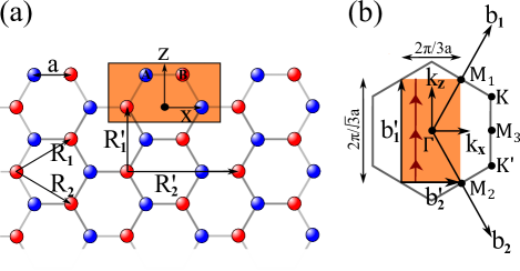
Figure 7: (a) Constant-y cross section of the crystal structure of KHgSb, with bulk Bravais lattice vectors $\boldsymbol{R}_{1}$ and $\boldsymbol{R}_{2}$. The top armchair edge is the cross-section of a glide-symmetric surface. A nonprimitive unit cell consistent with a glide-symmetric surface contains four atoms in both A and B sublattices (colored red and blue respectively); this nonprimitive cell, when translated by vectors $\boldsymbol{R}^{\prime}_{1}$ and $\boldsymbol{R}^{\prime}_{2}$, covers the entire xz-plane. Note that this nonprimitive unit cell has twice the volume of the primitive cell. (b) The hexagon illustrates the constant-$k_{z}$ cross-section of the BZ; $\boldsymbol{b}_{1}$ and $\boldsymbol{b}_{2}$ are primitive reciprocal vectors dual to $\boldsymbol{R}_{1}$ and $\boldsymbol{R}_{2}$; the orange rectangle inscribed in the hexagon illustrates BZ’, which is the Wigner-Seitz cell of a modified reciprocal lattice with basis vectors $\boldsymbol{b}_{1}^{\prime}$ and $\boldsymbol{b}_{2}^{\prime}$ (which are dual to $\boldsymbol{R}^{\prime}_{1}$ and $\boldsymbol{R}^{\prime}_{2}$).

Appendix D Material analysis: space groups and elementary band representations

D.1 Ba₂Pb

The space group of Ba₂Pb is SG62 ($Pnma$), which has an orthorhombic lattice. The spatial symmetries include: an inversion ($\cal I$), three screws ($\{C_{2x}|\frac{1}{2}\frac{1}{2}\frac{1}{2}\}$, $\{C_{2y}|0\frac{1}{2}0\}$ and $\{C_{2z}|\frac{1}{2}0\frac{1}{2}\}$), two glide ($g_{x}\equiv\{r_{x}|\frac{1}{2}\frac{1}{2}\frac{1}{2}\}$ and $g_{z}\equiv\{r_{z}|\frac{1}{2}0\frac{1}{2}\}$) and one mirror ($\{r_{y}|0\frac{1}{2}0\}$). Note $r_{j}$ is a mirror operation that inverts the single coordinate $j$.

For the calculations of topological invariants, we redefine the lattice vectors as $\vec{a}^{\prime}=2\vec{a}+\vec{b}$, $\vec{b}^{\prime}=b$ and $\vec{c}^{\prime}=c$, which are orthogonal. We can then set $a^{\prime},b^{\prime}$ and $c^{\prime}$ as the $x,y,z$ axes. With respect to these new lattice vectors, the glide symmetry is represented by $g_{x}\equiv\{r_{x}|00\frac{1}{2}\}$.

Beside exhibiting a nontrivial connectivity of the Zak phases [cf. Fig. 5(a)], another manifestationBradlyn et al. (2017); Alexandradinata and Höller (2018) of the nontriviality of Ba₂Pb is that its groundstate is not a direct sum of elementary band representations.Bradlyn et al. (2017); Alexandradinata and Höller (2018) To prove this, it is sufficient to compare the irreducible representations (irreps) at high-symmetry wavevectors.Bradlyn et al. (2017); Elcoro et al. (2017) By inspection, the irreps of Ba₂Pb (Tab. 2) cannot be decomposed into a direct sum of irreps of the elementary band representations, as obtained from the Bilbao crystallographic server (reproduced in Tab. 1).

Table 1: Elementary band representationsBradlyn et al. (2017); Elcoro et al. (2017) for SG62.

Wyckoff pos.	4a	4a	4b	4b	4c
Band-Rep.	$A_{g}A_{g}$	$A_{u}A_{u}$	$A_{g}A_{g}$	$A_{u}A_{u}$	${}^{1}E^{2}E$
$\Gamma$	4x5	4x6	4x6	4x6	4x6
R	(3+3)$\oplus$(4+4)	(3+3)$\oplus$(4+4)	(3+3)$\oplus$(4+4)	(3+3)$\oplus$(4+4)	(3+3)$\oplus$(4+4)
S	(3+3)$\oplus$(4+4)	(3+3)$\oplus$(4+4)	(3+3)$\oplus$(4+4)	(3+3)$\oplus$(4+4)	(3+3)$\oplus$(4+4)
T	2x(3+4)	2x(3+4)	2x(3+4)	2x(3+4)	2x(3+4)
U	2x(5+5)	2x(6+6)	2x(6+6)	2x(5+5)	(5+5)$\oplus$(6+6)
X	2x(3+4)	2x(3+4)	2x(3+4)	2x(3+4)	2x(3+4)
Y	2x(3+4)	2x(3+4)	2x(3+4)	2x(3+4)	2x(3+4)
Z	2x(3+4)	2x(3+4)	2x(3+4)	2x(3+4)	2x(3+4)

Table 2: Irreducible representations for Ba2Pb, as computed by VASP.

	Valence bands
$\Gamma$	6;5;6;5;5;6;5;6;6;5;6;6;
R	4+4;3+3;3+3;4+4;3+3;4+4;
S	4+4;3+3;3+3;4+4;4+4;3+3;
T	3+4;3+4;3+4;3+4;3+4;3+4;
U	5+5;6+6;6+6;5+5;6+6;5+5;
X	3+4;3+4;3+4;3+4;3+4;3+4;
Y	3+4;3+4;3+4;3+4;3+4;3+4;
Z	3+4;3+4;3+4;3+4;3+4;3+4;

D.2 Stressed Na₃Bi

For Na₃Bi that is stressed in the $x$ direction, the space group falls into $Cmcm$ (SG 63), which is a body-center structure. The conventional lattices are redefined as $\vec{a}^{\prime}=0.98(\vec{a}+\vec{b})$ where the factor 0.98 is due to a hypothetical compression in the x direction, $\vec{b}^{\prime}=b$ and $\vec{c}^{\prime}=c$, where $a,b,c$ are the primitive lattice vectors in the original structure(SG 194). $\chi^{+}$ is calculated with the conventional (non-primitive) lattices. The glide symmetry is represented by $g_{x}\equiv\{r_{x}|00\frac{1}{2}\}$.

By comparing the irreps of all elementary band representations [in SG63; see Tab. 3] with the irreps of stressed Na₃Bi [cf. Tab. 4], we conclude that the groundstate of stressed Na₃Bi is not band-representable.

Table 3: Elementary band representations for SG63.

Wyckoff pos.	4a	4a	4b	4b	4c
Band-Rep.	${}^{1}E_{g}^{2}E_{g}$	${}^{1}E_{u}^{2}E_{u}$	${}^{1}E_{g}^{2}E_{g}$	${}^{1}E_{u}^{2}E_{u}$	E
$\Gamma$	2x5	2x6	2x5	2x6	5+6
R	2+2	2+2	2+2	2+2	2+2
S	2x(3+4)	2x(5+6)	2x(5+6)	2x(3+4)	(3+4)$\oplus$(5+6)
T	3+4	3+4	3+4	3+4	3+4
Y	2x5	2x6	2x5	2x6	5+6
Z	3+4	3+4	3+4	3+4	3+4

Table 4: Irreducible representations for stressed Na3Bi, as computed by VASP.

	Valence bands
$\Gamma$	5;6;5;5;5+6;
R	8; 12; 11; 9; 8; 12;
S	5+6; 3+4; 3+4; 5+6; 3+4; 5+6;
T	3+4; 3+4; 3+4;
Y	5; 6; 6; 5; 6; 5;
Z	3+4; 3+4; 3+4;

D.3 KHgSb

The space group of KHgSb is $D_{6h}^{4}$ or SG194; further details about its crystallographic structure may be found in Ref. Wang et al., 2016. By comparing the irreps of all elementary band representations [in SG194; see Tab. 5] with the irreps of KHgSb [cf. Tab. 6], we conclude that the groundstate of KHgSb is not band-representable.

Table 5: Elementary band representations for SG194

Wyckoff pos.	2a	2a	2a	2a	2b	2b	2b	2c	2c	2c	2d	2d	2d
Band-Rep.	${}^{1}E_{g}^{2}E_{g}$	${}^{1}E_{u}^{2}E_{u}$	$E_{1g}$	$E_{1u}$	$E_{1}$	$E_{2}$	$E_{3}$	$E_{1}$	$E_{2}$	$E_{3}$	$E_{1}$	$E_{2}$	$E_{3}$
A	(4+5)	(4+5)	6	6	6	6	4+5	6	6	4+5	6	6	4+5
$\Gamma$	2x7	2x10	8$\oplus$9	11$\oplus$12	9$\oplus$11	8$\oplus$12	7$\oplus$10	9$\oplus$11	8$\oplus$12	7$\oplus$10	9$\oplus$11	8$\oplus$12	7$\oplus$10
H	(4+5)$\oplus$(6+7)	(4+5)$\oplus$(6+7)	8$\oplus$9	8$\oplus$9	8$\oplus$9	8$\oplus$9	(4+5)$\oplus$(6+7)	(4+5)$\oplus$9	(6+7)$\oplus$8	8$\oplus$9	(4+5)$\oplus$9	(6+7)$\oplus$8	8$\oplus$9
K	2x7	2x7	8$\oplus$9	8$\oplus$9	2x9	2x8	2x7	7$\oplus$8	7$\oplus$9	8$\oplus$9	7$\oplus$8	7$\oplus$9	8$\oplus$9
L	3+4	3+4	3+4	3+4	3+4	3+4	3+4	3+4	3+4	3+4	3+4	3+4	3+4
M	2x5	2x6	2x5	2x6	5+6	5+6	5+6	5+6	5+6	5+6	5+6	5+6	5+6

Table 6: Irreducible representations for KHgSb, as computed by VASP.

	Valence bands
A	6;6;6;
$\Gamma$	8;12; 11; 9; 8; 12;
H	6+7; 8; 9; 8; 6+7; 8;
K	7; 8; 9; 9; 7; 9;

Appendix E Ambiguity in the choice of coordinate systems

This appendix addresses a question posed at the end of Sec. IV, which we will briefly recapitulate. Suppose we choose a right-handed, Cartesian coordinate system where where $\vec{\boldsymbol{x}}$ (resp. $\vec{\boldsymbol{y}}$) lies parallel to the reflection (resp. fractional translational) component of the glide, i.e., the glide maps $(x,y,z)\rightarrow(-x,y\pm R_{2}/2,z)$. Such a coordinate system would be called glide-symmetric. Would the topological invariants $\chi^{+}$ (or ${\cal C}$) differ if measured in distinct glide-symmetric coordinates?

As argued in Sec. IV, there are three glide-symmetric coordinates which are related to each other by two-fold rotations $C_{2j}$ about the directional axes $\vec{j}$ ($j=x,y,z$); we shall only concern ourselves with proper point-group transformations that preserve the orientation (or handedness) of the coordinate system. We will refer to one glide-symmetric, right-handed (but otherwise arbitrarily chosen) coordinate system – in $\boldsymbol{k}$-space – as the reference coordinate system; all other coordinate systems are related to the reference by $\boldsymbol{k}^{\prime}=p\circ\boldsymbol{k}$, with $p$ a point-group transformation (e.g., $C_{2x}\circ\boldsymbol{k}:=(k_{x},-k_{y},-k_{z})$ etc). It should be emphasized that $p$ is not necessarily a symmetry of the solid (i.e., not an element of the space group), but merely reflects an ambiguity in the choice of coordinates.

To establish notation, a map between points: $\boldsymbol{k}\rightarrow p\circ\boldsymbol{k}$ induces naturally a map between subregions of the Brillouin torus (e.g., lines denoted as $l$, or faces denoted as $a,b,c,d$.); we shall denote this as $l\rightarrow p\circ l$ etc; several examples are illustrated in Fig. 8. It is useful (as an intermediate step in the following computations) to decompose $C_{2x}$ as the product of two reflections $r_{y}$ and $r_{z}$, such that each $r_{j}$ inverts only the $j$’th coordinate ($j=x,y,z$). We will also consider coordinate transformations induced by the inversion ${\cal I}:(x,y,z)\rightarrow(-x,-y,-z)$, though inversion symmetry need not belong in the space group.

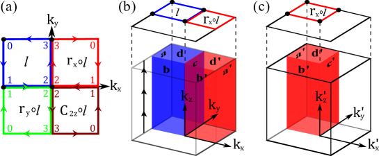
Figure 8: (a) Illustration of $p\circ l$ in the surface Brillouin torus. (b) Bent manifolds $abcd$ and $a^{\prime}b^{\prime}c^{\prime}d^{\prime}=r_{x}\circ abcd$ in the $\boldsymbol{k}$ coordinates; note that $r_{x}\circ c$ and $c$ differ only in orientation. (c) $r_{x}\circ abcd$ in the reflected coordinates $(k_{x}^{\prime},k_{y}^{\prime},k_{z}^{\prime})=(-k_{x},k_{y},k_{z}).$

We separately analyze the coordinate dependence of ${\cal C}$ and $\chi^{\pm}$ in Sec. E.1 and Sec. E.2 respectively.

E.1 Coordinate dependence of the bent Chern number ${\cal C}$

We begin by defining the Berry curvature as a pseudovector field $\boldsymbol{{\cal F}}=({\cal F}_{x},{\cal F}_{y},{\cal F}_{z})$, with components

$${{\cal F}_{a}=i\epsilon_{abc}\sum_{n=1}^{n_{\scriptscriptstyle{{occ}}}}\big{\langle}\partial_{b}u_{n}\big{|}\partial_{c}u_{n}\big{\rangle};}$$ (101)

$\partial_{j}$ is shorthand for the derivative with respect to $k_{j}$, $\epsilon_{abc}$ is the Levi-Cevita tensor, repeated indices (e.g., $b,c$ above) are summed over the Cartesian directions $x,y,z$. The bent Chern number is defined as the integral of the Berry curvature

$${{\cal C}=-\int_{|a|}{\cal F}_{x}dk_{y}dk_{z}-\int_{|b|}{\cal F}_{y}dk_{x}dk_{z}+\int_{|c|}{\cal F}_{x}dk_{y}dk_{z}+\int_{|d|}{\cal F}_{y}dk_{x}dk_{z};}$$ (102)

where $|f|$ in the subscript of $\int_{|f|}$ denotes the face $f$ without its orientation. The $\pm$ signs in front of each integral reflects our convention that ${\cal C}$ measures the outgoing Berry ‘flux’, or equivalently the net charge of the Berry monopoles within the quadrant enclosed by $abcd$. An equivalent and useful expression is

$${{\cal C}=\frac{i}{2\pi}\int_{0}^{4}\frac{dt}{4}\int_{0}^{2\pi}\frac{dk_{z}}{2\pi}\left[\big{\langle}\partial_{t}u\big{|}\partial_{k_{z}}u\big{\rangle}-\big{\langle}\partial_{k_{z}}u\big{|}\partial_{t}u\big{\rangle}\right],}$$ (103)

where $t\in[0,4]$ (with $4\equiv 0$) parametrizes the loop $l$ on which $abcd$ projects in the z direction, as illustrated in Fig. 8(a) [see also Fig. 2(b)]. $l$ is anticlockwise-oriented [as indicated by arrows in Fig. 8(a)], and $t$ increases in the direction of the orientation loop $l$.

Let ${\cal C}$ be the Chern number defined over $abcd$ in the reference coordinate system (parametrized by $\boldsymbol{k}$). We define $p\circ{\cal C}$ as the same Chern number in a different coordinate system parametrized by $\boldsymbol{k}^{\prime}=p\circ\boldsymbol{k}$; that is, $p\circ{\cal C}$ is defined exactly as in Eq. (102) but with $\boldsymbol{k}$ replaced by $\boldsymbol{k}^{\prime}$. For the same Hamiltonian, we would prove that

$${{\cal C}=r_{x}\circ{\cal C}=r_{y}\circ{\cal C}=-r_{z}\circ{\cal C}.}$$ (104)

To prove the first equality, consider that $r_{x}\circ{\cal C}$ is the Chern number defined over $a^{\prime}b^{\prime}c^{\prime}d^{\prime}{=}r_{x}\circ abcd$ in the $\boldsymbol{k}^{\prime}=(-k_{x},k_{y},k_{z})$ coordinates, as illustrated in Fig. 8(c). In the reference coordinates, $a^{\prime}b^{\prime}c^{\prime}d^{\prime}$ is comparatively illustrated with $abcd$ in Fig. 8(b). Since $a^{\prime}b^{\prime}c^{\prime}d^{\prime}$ and $abcd$ are related by the reflection $r_{x}$, they enclose different quadrants of the BZ (colored red and blue respectively). To deduce that ${\cal C}=r_{x}\circ{\cal C}$, we will rely on two observations: (i) While $r_{x}\circ{\cal C}$ is defined to measure the outgoing Berry flux in the $\boldsymbol{k}^{\prime}$ coordinates, it measures the incoming Berry flux in the reference coordinates $\boldsymbol{k}$; this may be deduced by the $r_{x}\circ l$ having an opposite orientation relative to $l$, as illustrated in Fig. 8 (a- b). (ii) Since the curvature transforms like pseudovector, we expect that glide-related Berry monopoles having opposite charge – therefore the net monopole charge in the blue quadrant is negative the monopole charge in the red quadrant. In combination, (i-ii) produces the desired result.

${\cal C}=r_{y}\circ{\cal C}$ [the second equality in Eq. (104)] may be derived by a simple generalization of the above argument. Now the two quadrants (enclosed by $abcd$ and $r_{y}\circ abcd$) are related by a composition ($Tg_{x}$) of time-reversal and glide symmetry. (i’) $r_{y}\circ{\cal C}$ also measures the incoming Berry flux in the reference coordinates, and (ii’) $Tg_{x}$-related monopoles have opposite charge. (Note that $r_{y}$ is not assumed be a symmetry in the space group, but if it were, we would similarly conclude that $r_{y}$-related monopoles have opposite charge.)

${\cal C}=-r_{z}\circ{\cal C}$ [the last equality in Eq. (104)] may be derived from the following argument. When both $abcd$ and $a^{\prime}b^{\prime}c^{\prime}d^{\prime}=r_{z}\circ abcd$ are viewed in the reference coordinates, the two surfaces occupy the same area (in $\boldsymbol{k}$-space) and differ only in their orientations; this difference in orientations originates from the reversal of $k_{z}$. This implies that $r_{z}\circ{\cal C}$ measures the incoming Berry flux through $abcd$.

From Eq. (104) and $C_{2x}=r_{y}r_{z}$ etc., we derive that the bent Chern numbers – for two coordinate parametrizations of the same Hamiltonian – are related as

$$p\circ{\cal C}=\begin{cases}-{\cal C},&p\in\{C_{2x},C_{2y}\},\\ {\cal C},&p=C_{2z}.\end{cases}$$ (105)

E.2 Coordinate dependence of topological invariant $\chi^{\pm}$

Let us define $\chi^{\pm}$ as $\mathbb{Z}_{4}$ invariants defined with respect to a reference coordinate system parametrized by $\boldsymbol{k}$; analogously, $p\circ\chi^{\pm}$ are defined as the $\mathbb{Z}_{4}$ invariants defined with respect to a distinct coordinate system with $\boldsymbol{k}^{\prime}=p\circ\boldsymbol{k}$. For the same Hamiltonian, we will show that

$$p\circ\chi^{\pm}=\begin{cases}-\chi^{\mp},&p\in\{C_{2x},C_{2y}\},\\ \chi^{\pm},&p=C_{2z}.\end{cases}$$ (106)

This would imply, in combination with Eq. (105), that $\chi^{+}+\chi^{-}\equiv 2{\cal C}$ mod $4$ [cf. Eq. (3)] is invariant under proper coordinate transformations – a result applicable to both band insulators and Weyl metals.

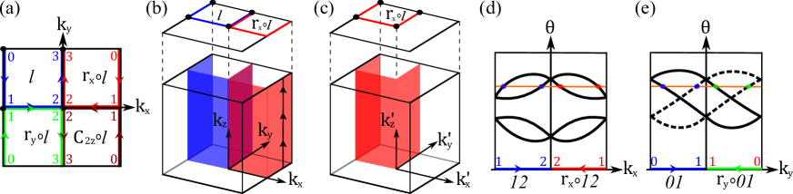
Figure 9: (a) Illustration of $p\circ l$ in the surface Brillouin torus. (b) Bent subregions on which the $\mathbb{Z}_{4}$ invariants $\chi[p\circ l]$ are defined. (c) Bent subregion in which $r_{x}\circ\chi^{\pm}[l]$ is defined, in the reflected coordinates $(k_{x}^{\prime},k_{y}^{\prime},k_{z}^{\prime})=(-k_{x},k_{y},k_{z}).$ (d) Representative Zak-phase dispersion along $12$ and $r_{x}\circ 12$. (e) Representative Zak-phase dispersion along $01$ and $r_{y}\circ 01$.

The rest of this appendix is devoted to proving Eq. (106). Let $l$ be the oriented path in $(k_{x},k_{y})$-space on which $\chi^{\pm}[l]$ is defined through Eq. (LABEL:wilsonex). $l$ is illustrated in Fig. 9(a), in conjunction with the three other point-group mapped $p\circ l$; we remind the reader that $p$ is not necessarily a symmetry of the solid. A word of caution: $l$ was also used in the previous section to define a loop illustrated in Fig. 8; in this section we use the same symbol $l$ for an open segment of the loop in Fig. 8.

For each of $p\circ l$ illustrated in Fig. 9(a), we define the quantities $\chi^{\pm}[p\circ l]$ which simply generalize our original definition in Eq. (LABEL:wilsonex):

Eq. (LABEL:wilsonex) is a particularization of $\chi^{\pm}[p\circ l]$ for $p$ being the identity operation. Here, we have parametrized $p\circ l(t)$ by $t\in[0,3]$ such that $t\in\{0,1,2,3\}$ lie on the high-symmetry wavevectors in the $k_{x}-k_{y}$ plane, as illustrated in Fig. 9(a). $\{e^{i\theta_{j}[p\circ l(t)]}\}$ are eigenvalues of the Wilson loop – for an oriented quasimomentum loop which projects in the z direction to the wavevector $p\circ l(t)$, as illustrated by the triple arrows in Fig. 9(b); by definition, the orientation of each loop is always in the direction of increasing $k_{z}$.

In congruence with our previous definitions, $\chi^{\pm}[p_{1}\circ l]$ is defined respect to a reference coordinate $\boldsymbol{k}$, and we define $p_{2}\circ\chi^{\pm}[p_{1}\circ l]$ with respect to $\boldsymbol{k}^{\prime}=p_{2}\circ\boldsymbol{k}$, with $p_{1}$ not necessarily equal to $p_{2}$. We caution that $\chi^{\pm}[p\circ l]$ and $p\circ\chi^{\pm}[l]$ are not necessarily equal, as will be seen in Eq. (115).

E.2.1 Proposition 1

Let us prove an intermediate proposition:

$${\chi^{\pm}[l]\equiv\chi^{\pm}[r_{x}\circ l]\equiv\chi^{\mp}[r_{y}\circ l]\equiv\chi^{\mp}[C_{2z}\circ l],}$$ (107)

where $\equiv$ is an equivalence modulo four.

Let us introduce the shorthand $p\circ j(j+1)$, for $j\in\{0,1,2\}$, as the subset of $p\circ l(t)$ in which $t\in[j,j+1]$. That is, $l$ is the union of intervals $01$, $12$ and $23$, and so similarly we define $p\circ 01$, $p\circ 12$ and $p\circ 23$ for $p\circ l$. The relation in Eq. (1) simply generalizes to

$${\chi^{\pm}[p\circ l]\equiv 2{\cal S}^{\pm}_{p\circ 01}(\bar{\theta})+{\cal S}_{p\circ 12}(\bar{\theta})+2{\cal S}^{\pm}_{p\circ 23}(\bar{\theta}).}$$ (108)

where ${\cal S}_{p\circ ij}$ is defined analogously to ${\cal S}_{ij}$, as introduced in the main text. We write it down for clarity: draw a constant-$\bar{\theta}$ reference line (for an arbitrarily chosen Zak phase $\bar{\theta}$) and consider its intersections with Zak bands along $p\circ l$. For each intersection between $p\circ 12$, we calculate the sign of the velocity $d\theta/dt$, and sum this quantity over all intersections to obtain ${\cal S}_{p\circ 12}(\bar{\theta})$; for $p\circ 01$ and $p\circ 23$, we consider only intersections with Zak bands in the $\Delta_{\pm}$ representation, and we similary sum over sgn[$d\theta/dt$] to obtain ${\cal S}^{\pm}_{p\circ 01}(\bar{\theta})$ and ${\cal S}^{\pm}_{p\circ 23}(\bar{\theta})$ respectively.

Proof of $\chi^{\pm}[l]\equiv\chi^{\pm}[r_{x}\circ l]$

Along the glide-invariant lines, $r_{x}\circ 01=01$ and $r_{x}\circ 23=23$, and therefore ${\cal S}^{\pm}_{r_{x}\circ 01}={\cal S}^{\pm}_{01}$ and ${\cal S}^{\pm}_{r_{x}\circ 23}={\cal S}^{\pm}_{23}$. However, $r_{x}\circ 12{\neq}12$ lie on distinct lines which are related by time-reversal symmetry [which maps $(k_{x},k_{y})\rightarrow(-k_{x},-k_{y})$], as illustrated in Fig. 9(a). This symmetry imposes ${\cal S}_{12}={\cal S}_{r_{x}\circ 12}$, as we now explain. Suppose a Zak band over $12$ intersects our constant-$\bar{\theta}$ line with velocity $v$, then its time-reversed partner is a Zak band over $r_{x}\circ 12$, which intersects the $\bar{\theta}$ line with velocity $-v$. By $v$ and $-v$, we refer to velocities defined by varying the Zak phase of a Zak band with respect to $k_{x}$. However, our definition of ${\cal S}_{p\circ ij}$ involved velocities defined by varying the Zak phase with respect to a parameter that is specific to $p\circ ij$: the parameter for $12$ increases in the same direction as $k_{x}$, but the parameter for $r_{x}\circ 12$ increases in the opposite direction, as illustrated in Fig. 9(a) and (d). Therefore, each pair of time-reversed Zak bands contribute equally to ${\cal S}_{12}$ and ${\cal S}_{r_{x}\circ 12}$, leading to ${\cal S}_{12}={\cal S}_{r_{x}\circ 12}$. For example, consider a representative Zak-band dispersion in Fig. 9(d), where ${\cal S}_{12}={\cal S}_{r_{x}\circ 12}=2$ for the chosen reference line (colored orange). $\blacksquare$

Proof of $\chi^{\pm}[l]\equiv\chi^{\mp}[r_{y}\circ l]$

Since $12=r_{y}\circ 12$,

$${{\cal S}_{12}={\cal S}_{r_{y}\circ 12}.}$$ (109)

Time reversal relates $01$ and $r_{y}\circ 01$, are therefore imposes a relation between ${\cal S}^{\pm}_{01}$ and ${\cal S}^{\pm}_{r_{y}\circ 01}$, as we now derive. Recall from Sec. A.2 that time-reversed partner states at $\pm k_{y}$ belong to opposite representations $\Delta_{\pm}$ of the glide $g_{x}$. This implies that (a) a Zak band in the $\Delta_{\pm}$ representation at $01$ has a time-reversed partner at $r_{y}\circ 01$ in the $\Delta_{\mp}$ representation; note that $01$ and $r_{y}\circ 01$ are distinct lines in $\boldsymbol{k}$-space. (b) Moreover, as representatively illustrated in Fig. 9(e), time-reversed partners have opposite-sign velocities with respect to variation of $k_{y}$, but equal velocities with respect to varying the parameters of $01$ and $r_{y}\circ 01$ respectively. (a) and (b) together imply

$${{\cal S}_{01}^{\pm}={\cal S}_{r_{y}\circ 01}^{\mp}.}$$ (110)

By cosmetic substitution of $12\rightarrow 23$ in the above demonstration, we would show that

$${{\cal S}_{23}^{\pm}={\cal S}_{r_{y}\circ 23}^{\mp}.}$$ (111)

Eq. (109), Eq. (110), Eq. (111) and Eq. (108) together imply our claim. $\blacksquare$

Finally, $\chi^{\pm}[l]\equiv\chi^{\mp}[C_{2z}\circ l]$ may be proven from

$${{\cal S}_{12}={\cal S}_{C_{2z}\circ 12},\;\;\;\;{\cal S}_{01}^{\pm}={\cal S}_{C_{2z}\circ 01}^{\mp},\;\;\;\;{\cal S}_{23}^{\pm}={\cal S}_{C_{2z}\circ 23}^{\mp}.}$$ (112)

E.2.2 Dependence on proper coordinate transformations

Let the $p$ be a proper point-group transformation that preserves handedness of the coordinate system. $p$ can always be viewed as the composition of a two-dimensional point-group operation ($p_{\perp}$) acting in the $k_{x}-k_{y}$ plane, and a one-dimensional point group operation acting in the $k_{z}$ line:

$${p\circ\boldsymbol{k}=(p_{\perp}\circ(k_{x},k_{y}),p_{\parallel}k_{z}),\;\;\;\;p_{\parallel}\in\pm 1.}$$ (113)

This gives a correspondence $p\leftrightarrow(p_{\perp},p_{\parallel})$. We are particularly interested in

$${C_{2x}\leftrightarrow(r_{y},-1),\;\;\;\;C_{2y}\leftrightarrow(r_{x},-1),\;\;\;\;C_{2z}\leftrightarrow(C_{2z},+1).}$$ (114)

For two coordinate parametrizations ($\boldsymbol{k}$ and $\boldsymbol{k}^{\prime}=p\circ\boldsymbol{k}$) of the same Hamiltonian, we argue that

$${p\circ\chi^{\pm}[l,k_{z}]=\chi^{\pm pr_{x}p^{-1}r_{x}^{-1}}[p_{\perp}\circ l,p_{\parallel}k_{z}],}$$ (115)

where $\chi^{\pm}[p\circ l,k_{z}]:=\chi^{\pm}[p\circ l]$ as defined in Eq. (E.2), and $\chi^{\pm}[p\circ l,k_{z}]$ is identical to $\chi^{\pm}[p\circ l]$ except that the orientation of each Wilson loop is reversed (from increasing $k_{z}$ to decreasing $k_{z}$). The above equation has the following justification:

(i) A coordinate transformation effectively changes the bent quasimomentum region on which $\chi$ is calculated; this is reflected in a change in the argument of $\chi$. For example, $r_{x}\circ\chi^{\pm}[l,k_{z}]$ is defined over the bent quasimomentum subregion $a^{\prime}b^{\prime}c^{\prime}=r_{x}\circ abc$ that we illustrate in the primed coordinates [red sheet in Fig. 9(c)] and reference coordinates [red sheet in Fig. 9(b)]; $r_{x}\circ abc$ projects in the z direction to $r_{x}\circ l$.

(ii) Whether the glide representation changes under a coordinate transformation $(x,y,z)\rightarrow(x^{\prime},y^{\prime},z^{\prime})=p\circ(x,y,z)$ depends on $p$. To appreciate this, let us recall that the reflection component ($r_{x}$) of glide $g_{x}$ has an associated orientation. Indeed, $r_{x}$ may be viewed as the composition of a spatial inversion (${\cal I}$) with the two-fold rotation ($C_{2x}$) about the $x$-axis, and, for half-integer-spin representations, we need to specify if this rotation is clockwise- or anticlockwise-oriented. That is to say, a $\pi$ clockwise rotation differs from a $\pi$ anticlockwise rotation by a $-1$ phase factor. Consequently, the same glide-invariant state has glide eigenvalues with opposite signs – with respect to two glide operations which differ only in orientation. For a coordinate system $(x,y,z)$, we always define $g_{x}$ with a clockwise rotation about the $x$-axis; this was implicit in our previous definitions of $\Delta_{\pm}$ and $\chi^{\pm}$. Suppose a Bloch state transforms under $g_{x}$ with eigenvalue $\Delta_{\pm}=\pm ie^{-ik_{y}/2}$; the same state may (or may not) transform with the inverted eigenvalue $\mp ie^{-ik_{y}/2}$ under the glide $g_{x^{\prime}}$, which is defined with a clockwise orientation about the $x^{\prime}$-axis [recall $(x^{\prime},y^{\prime},z^{\prime})=p\circ(x,y,z)$]. The glide eigenvalue is inverted if and only if the coordinate transformation $p$ inverts the orientation of a rotation about the $x$-axis, i.e., it depends on $pr_{x}p^{-1}r_{x}^{-1}=\pm 1$ (with $-1$ indicating an inversion). For example, if $p=C_{2x}$, $g_{x^{\prime}}$ and $g_{x}$ have the same orientations; if $p=C_{2y}$, $g_{x^{\prime}}$ and $g_{x}$ have opposite orientations, because $r_{x}$ and $C_{2y}$ anticommute in the half-integer-spin representation. This possible change in the glide representation is accounted for in Eq. (115) by the superscript of $\chi$.

Beginning from Eq. (115), the next step is to express

$${p\circ\chi^{\pm}[l,k_{z}]\equiv p_{\parallel}\chi^{\pm pr_{x}p^{-1}r_{x}^{-1}}[p_{\perp}\circ l,k_{z}].}$$ (116)

To justify this, $p_{\parallel}=-1$ implies that the orientation of the Wilson loop flips, thus $e^{i\theta}(t)\rightarrow e^{-i\theta}(t)$, and the velocities at the reference Zak phase are likewise inverted; cf. Eq. (108).

Finally, inserting Eq. (114) and Eq. (107) [which should be understood as relating $\chi$ with constant $k_{z}$ arguments] into Eq. (116), we obtain

Within the classical approximation, and for the above-stated conditions on the light source, Fresnel’s equationsJackson (1999) inform us that the photon field within the solid remains linearly polarized, with a polarization vector $\vec{\epsilon}$ (within the solid) that is identical to the polarization vector of the light source.

In the temporal gauge, the electric field and vector potential are parallel, hence $\boldsymbol{a}$ (the screened vector potential within the solid) is proportional to $\vec{\epsilon}$. So far as we are concerned only with the absorption of photons, $\boldsymbol{a}$ (occurring in the electron-photon coupling $H_{int}$) may be equated with $a_{0}\vec{\epsilon}e^{i\boldsymbol{q}\cdot\boldsymbol{r}}$, where $a_{0}$ is a spatially-independent constant, and $\boldsymbol{q}$ is the wavevector of the photon within the solid.

For normally-incident light ($\boldsymbol{q}{=}{-}\omega\vec{z}/c$) with the polarization vector parallel to the glide plane ($\epsilon{=}\vec{y}$), $H_{int}$ commutes with the glide operation $\hat{g}_{x}$.

If the polarization vector is orthogonal to the glide plane ($\vec{\epsilon}{=}\vec{x}$), $H_{int}$ anticommutes with $\hat{g}_{x}$ in the case of normal incidence.

For non-normal incidence and $\vec{\epsilon}{=}\vec{x}$, $\hat{g}_{x}H_{int}\hat{g}_{x}^{-1}{=}{-}e^{-iq_{y}R_{2}/2}H_{int}$; the $q_{y}$-dependent phase factor originates from the half-lattice translation ($y{\rightarrow}y{-}R_{2}/2$) in $\hat{g}_{x}$.

F.2 Oblique incidence (parallel alignment)

As explained in the previous Sec. LABEL:sec:classicalmaxwell, the classical approximation is not satisfied if the incident electric field has a component normal to the surface – as would be the case for $p$-polarized radiation at oblique incidence.Feibelman (1976); Levinson et al. (1979); Feibelman (1982)

Nevertheless, so long as the optical response of the medium is linear (though not necessarily localFeibelman (1982)), the electron coupling to the medium-induced electromagnetic field (given by vector potential $\boldsymbol{a}^{ind}$) transforms in the same glide representation as the electron coupling to the externally applied field (given by $\boldsymbol{a}^{ext}$). That is to say, if $\hat{g}_{x}\boldsymbol{p}\cdot\boldsymbol{a}^{ext}\hat{g}_{x}^{-1}=e^{-iq_{y}R_{2}/2}\boldsymbol{p}\cdot\boldsymbol{a}^{ext}$, so must $\hat{g}_{x}\boldsymbol{p}\cdot\boldsymbol{a}^{ind}\hat{g}_{x}^{-1}=e^{-iq_{y}R_{2}/2}\boldsymbol{p}\cdot\boldsymbol{a}^{ind}$. This follows from the assumed existence of a linear functional relating the two potentials:

$${a_{i}^{ind}(\boldsymbol{r})=\sum_{j=x,y,z}\int\chi_{ij}(\boldsymbol{r},\boldsymbol{r}^{\prime})a_{j}^{ext}(\boldsymbol{r}^{\prime})d\boldsymbol{r}^{\prime},}$$ (117)

with the susceptibility satisfying the glide-symmetric constraint:

$$\chi_{ij}(\boldsymbol{r},\boldsymbol{r}^{\prime})=\sum_{a,b}[\mathfrak{r}_{x}]_{ia}[\mathfrak{r}_{x}]_{jb}\chi_{ij}(g_{x}\circ\boldsymbol{r},g_{x}\circ\boldsymbol{r}^{\prime}),\;\;\mathfrak{r}_{x}:=\begin{pmatrix}-1&0&0\\ 0&1&0\\ 0&0&1\end{pmatrix},\;\;g_{x}\circ(x,y,z):=(-x,y-R_{2}/2,z).$$ (118)

Consequently, the electron coupling to the total photon field transforms as $\hat{g}_{x}H_{int}\hat{g}_{x}^{-1}=e^{-iq_{y}R_{2}/2}H_{int}$.

References

- Wang et al. (2016) Z. Wang, A. Alexandradinata, R. J. Cava, and B. A. Bernevig, Nature 532, 189 (2016).
- Alexandradinata et al. (2016) A. Alexandradinata, Z. Wang, and B. A. Bernevig, Phys. Rev. X 6, 021008 (2016).
- Shiozaki et al. (2016) K. Shiozaki, M. Sato, and K. Gomi, Phys. Rev. B 93, 195413 (2016).
- Ma et al. (2017) J. Ma, C. Yi, B. Lv, Z. Wang, S. Nie, L. Wang, L. Kong, Y. Huang, P. Richard, P. Zhang, K. Yaji, K. Kuroda, S. Shin, H. Weng, B. A. Bernevig, Y. Shi, T. Qian, and H. Ding, Science Advances 3 (2017), 10.1126/sciadv.1602415.
- Fang and Fu (2015) C. Fang and L. Fu, Phys. Rev. B 91, 161105 (2015).
- Shiozaki et al. (2015) K. Shiozaki, M. Sato, and K. Gomi, Phys. Rev. B 91, 155120 (2015).
- Liu et al. (2014) C.-X. Liu, R.-X. Zhang, and B. K. VanLeeuwen, Phys. Rev. B 90, 085304 (2014).
- Ezawa (2016) M. Ezawa, Phys. Rev. B 94, 155148 (2016).
- (9) P.-Y. Chang, O. Erten, and P. Coleman, Nature Physics (2017) doi:10.1038/nphys4092 .
- (10) L. Lu, C. Fang, L. Fu, S. G. Johnson, J. D. Joannopoulos, and M. Soljacic, Nature Physics (2016) doi:10.1038/nphys3611 .
- Kruthoff et al. (2017) J. Kruthoff, J. de Boer, J. van Wezel, C. L. Kane, and R.-J. Slager, Phys. Rev. X 7, 041069 (2017).
- Bradlyn et al. (2017) B. Bradlyn, L. Elcoro, J. Cano, M. G. Vergniory, Z. Wang, C. Felser, M. I. Aroyo, and B. A. Bernevig, Nature 547, 298 (2017), article.
- Wieder et al. (2017) B. J. Wieder, B. Bradlyn, Z. Wang, J. Cano, Y. Kim, H.-S. D. Kim, A. M. Rappe, C. L. Kane, and B. A. Bernevig, ArXiv e-prints (2017), arXiv:1705.01617 [cond-mat.mes-hall] .
- Lax (1974) M. Lax, Symmetry principles in solid state and molecular physics (Wiley-Interscience, Corporate Headquarters 111 River Street, Hoboken, NJ 07030-5774, USA, 1974).
- Fu et al. (2007) L. Fu, C. L. Kane, and E. J. Mele, Phys. Rev. Lett. 98, 106803 (2007).
- Moore and Balents (2007) J. E. Moore and L. Balents, Phys. Rev. B 75, 121306 (2007).
- Roy (2009a) R. Roy, Phys. Rev. B 79, 195322 (2009a).
- Fu and Kane (2007) L. Fu and C. L. Kane, Phys. Rev. B 76, 045302 (2007).
- Xiong and Alexandradinata (2018) C. Z. Xiong and A. Alexandradinata, Phys. Rev. B 97, 115153 (2018).
- Note (1) This deformation argument was first presented in Ref. \rev@citealpnumNonsymm_Shiozaki.
- Cardona and Ley (1978) M. Cardona and L. Ley, Photoemission in Solids I (Springer-Verlag, Berlin, Heidelberg, New York, 1978).
- Hufner (2003) S. Hufner, Photoelectron spectroscopy (Springer, 2003).
- Fidkowski et al. (2011) L. Fidkowski, T. S. Jackson, and I. Klich, Phys. Rev. Lett. 107, 036601 (2011).
- Huang and Arovas (2012) Z. Huang and D. P. Arovas, Phys. Rev. B 86, 245109 (2012).
- Wang et al. (2012) Z. Wang, Y. Sun, X.-Q. Chen, C. Franchini, G. Xu, H. Weng, X. Dai, and Z. Fang, Phys. Rev. B 85, 195320 (2012).
- Sun et al. (2011) Y. Sun, X.-Q. Chen, C. Franchini, D. Li, S. Yunoki, Y. Li, and Z. Fang, Phys. Rev. B 84, 165127 (2011).
- Gobeli et al. (1964) G. W. Gobeli, F. G. Allen, and E. O. Kane, Phys. Rev. Lett. 12, 94 (1964).
- Hermanson (1977) J. Hermanson, Solid State Communications 22, 9 (1977).
- Pescia et al. (1985) D. Pescia, A. Law, M. Johnson, and H. Hughes, Solid State Communications 56, 809 (1985).
- Prince (1987) K. Prince, Journal of Electron Spectroscopy and Related Phenomena 42, 217 (1987).
- Borstel et al. (1981) G. Borstel, M. Neumann, and M. Wöhlecke, Phys. Rev. B 23, 3121 (1981).
- Fang et al. (2012) C. Fang, M. J. Gilbert, X. Dai, and B. A. Bernevig, Phys. Rev. Lett. 108, 266802 (2012).
- Atala (2013) M. Atala, et al., Nature Physics 9, 795 (2013).
- Li et al. (2015) T. Li, L. Duca, M. Reitter, F. Grusdt, E. Demler, M. Endres, M. Schleier-Smith, I. Bloch, and U. Schneider, (2015), arXiv:1509.02185 .
- Soluyanov and Vanderbilt (2011a) A. A. Soluyanov and D. Vanderbilt, Phys. Rev. B 83, 235401 (2011a).
- Yu et al. (2011) R. Yu, X. L. Qi, A. Bernevig, Z. Fang, and X. Dai, Phys. Rev. B 84, 075119 (2011).
- Alexandradinata et al. (2014a) A. Alexandradinata, X. Dai, and B. A. Bernevig, Phys. Rev. B 89, 155114 (2014a).
- Wilczek and Zee (1984) F. Wilczek and A. Zee, Phys. Rev. Lett. 52, 2111 (1984).
- Höller and Alexandradinata (2018) J. Höller and A. Alexandradinata, Phys. Rev. B 98, 024310 (2018).
- Wan et al. (2011) X. Wan, A. Turner, A. Vishwanath, and S. Y. Savrasov, Phys. Rev. B 83, 205101 (2011).
- Halasz and Balents (2012) G. B. Halasz and L. Balents, Phys. Rev. B 85, 035103 (2012).
- Alexandradinata et al. (2014b) A. Alexandradinata, C. Fang, M. J. Gilbert, and B. A. Bernevig, Phys. Rev. Lett. 113, 116403 (2014b).
- Note (2) This is distinct from the noncrystalline, strong invariantFu et al. (2007); Moore and Balents (2007).
- C. L. Kane and E. J. Mele (2005) C. L. Kane and E. J. Mele, Phys. Rev. Lett. 95, 226801 (2005).
- Note (3) In principle we could consider the Kane-Mele invariants defined over four time-reversal-invariant planes, which project respectively to . However, given the strong invariant , only one of the four is independent. To appreciate this, note that the parity of uniquely determines strong invariant of 3D time-reversal-symmetric insulators.Xiong and Alexandradinata (2018) Precisely, mod 2 , where corresponds to the nontrivial phase. Moreover, is uniquely determined by the Kane-Mele invariants on parallel planes: .Yu et al. (2011) Due to and time-reversal symmetries, .Xiong and Alexandradinata (2018) Consequently, and is determined uniquely by and .
- Roy (2009b) R. Roy, Phys. Rev. B 79, 195321 (2009b).
- Fu and Kane (2006) L. Fu and C. L. Kane, Phys. Rev. B 74, 195312 (2006).
- Zak (1981) J. Zak, Phys. Rev. B 23, 2824 (1981).
- Evarestov and Smirnov (1984) R. A. Evarestov and V. P. Smirnov, Phys. Stat. Sol 122, 231 (1984).
- Bacry (1993) H. Bacry, Commun. Math. Phys. 153, 359 (1993).
- Alexandradinata and Höller (2018) A. Alexandradinata and J. Höller, ArXiv e-prints (2018), arXiv:1804.04131 [cond-mat.mes-hall] .
- Chen et al. (2017) D. Chen, T.-T. Zhang, C.-J. Yi, Z.-D. Song, W.-L. Zhang, T. Zhang, Y.-G. Shi, H.-M. Weng, Z. Fang, P. Richard, and H. Ding, Phys. Rev. B 96, 064102 (2017).
- Note (4) Any solid that is symmetric under would also be symmetric under , since is also a symmetry of the solid.
- Mahan (1970) G. D. Mahan, Phys. Rev. B 2, 4334 (1970).
- Note (5) These are not symmetries of a spin-orbit-coupled solid.
- Lippmann and Schwinger (1950) B. A. Lippmann and J. Schwinger, Phys. Rev. 79, 469 (1950).
- Gell-Mann and Goldberger (1953) M. Gell-Mann and M. L. Goldberger, Phys. Rev. 91, 398 (1953).
- Bethe and Salpeter (1957) H. A. Bethe and E. Salpeter, Quantum Mechanics of One- and Two-Electron Atoms (Springer-Verlag, Berlin, Goettingen, Heidelberg, 1957).
- Adawi (1964) I. Adawi, Phys. Rev. 134, A788 (1964).
- Feibelman and Eastman (1974) P. J. Feibelman and D. E. Eastman, Phys. Rev. B 10, 4932 (1974).
- Foldy and Wouthuysen (1950) L. L. Foldy and S. A. Wouthuysen, Phys. Rev. 78, 29 (1950).
- Blount (1962) E. I. Blount, Phys. Rev. 128, 2454 (1962).
- Ashcroft and Mermin (1976) N. W. Ashcroft and N. D. Mermin, Solid state physics (Thomson Learning, 20 Channel Center Street, Boston, MA 02210, USA, 1976).
- Note (6) may be derived by a simple generalization of Adawi’s calculationAdawi (1964) to include the effect of spin. The essential structure of the derivation is identical; one merely has to include a spin-orbit-coupling and Darwin terms to in Eq. (2.1) of Ref. \rev@citealpnumadawi_theoryphotoelectric, and to interpret in Eq. (2.3) as a spinor state.
- Feibelman (1982) P. J. Feibelman, Progress in Surface Science 12, 287 (1982).
- Feuchtwang et al. (1978) T. Feuchtwang, P. Cutler, and D. Nagy, Surface Science 75, 490 (1978).
- Feder (2013a) R. Feder, “Principles and theory of electron scattering and photoemission,” in Polarized Electrons in Surface Physics (WORLD SCIENTIFIC, 2013) pp. 125–241.
- Note (7) Because and is a unitary operator.
- Griffiths (2005) D. J. Griffiths, Introduction to quantum mechanics (Pearson Prentice Hall, Upper Saddle River, New Jersey, USA, 2005).
- Note (8) In practice, this domain may be even smaller due to a short photoelectron escape depth, and possibly also the finite cross-sectional area of the photon beam.
- Note (9) In an LEED experiment, an electron beam is directed to and diffracted off the surface of a solid. It is well-knownAdawi (1964); Mahan (1970); Feibelman and Eastman (1974) that is the spinless wavefunction for an LEED experiment in which the incident electron beam has momentum ; this wavefunction shall be referred to as an LEED state. In the spinless theory, the inverse-LEED state can be defined as the time-reversed LEED state; time-reversal has the effect of inverting momentum and sending , thus producing the spinless analog of Eq. (LABEL:lippPhi). In our spinful theory, the LEED state () describes an incoming, spin-polarized electron beam with momentum , and the inverse LEED state [right-hand side of Eq. (LABEL:lippPhi)] describes an outgoing beam with inverted momentum () but the same spin polarization .
- Ackermann and Feder (1985) B. Ackermann and R. Feder, Journal of Physics C: Solid State Physics 18, 1093 (1985).
- Ginatempo et al. (1985) B. Ginatempo, P. J. Durham, B. L. Gyorffy, and W. M. Temmerman, Phys. Rev. Lett. 54, 1581 (1985).
- Pendry (1976) J. Pendry, Surface Science 57, 679 (1976).
- Note (10) We are describing the physically-motivated scattering geometry in Fig. 6(a), where the sample is finite in all three directions. Rigorously, surface-parallel translations and glide cannot be symmetries of any surface with finite area. Practically, if the sample area is macroscopic, the effect of corners and edges are negligible to a state whose wavefunction is extended in and . Assuming that is such an extended state, it may be characterized to a good approximation by the symmetries of a semi-infinite solid (with a single surface); the unitary subgroup of such symmetries is denoted .
- Kirschner (2013) J. Kirschner, “Sources and detectors for polarized electrons,” in Polarized Electrons in Surface Physics (WORLD SCIENTIFIC, 2013) pp. 245–286.
- Scheidt et al. (1983) H. Scheidt, M. Glöbl, V. Dose, and J. Kirschner, Phys. Rev. Lett. 51, 1688 (1983).
- Kirschner (1984a) J. Kirschner, Surface Science 138, 191 (1984a).
- Kirschner et al. (1984) J. Kirschner, D. Rebenstorff, and H. Ibach, Phys. Rev. Lett. 53, 698 (1984).
- Kirschner (1984b) J. Kirschner, Solid State Communications 49, 39 (1984b).
- Note (11) Even in noncentrosymmetric space groups, certain other point-group symmetries might result in energy-degenerate initial states that have the same reduced wavevector () but belong in distinct glide representations. For example, a reflection symmetry (that inverts ) anticommutes with glide in the spinor representation; hence relates two energy-degenerate states [at ] that belong to distinct representations of .
- Note (12) This may be derived from a simple generalization of our theory. Second-order processes are either quadratic in or linear in , with for the parallel alignment and for the anti-parallel alignment. For either alignment, and are invariant under the glide operation, hence the photoelectron has the same glide representation as the initial state.
- Feder (2013b) R. Feder, Polarized Electrons in Surface Physics (WORLD SCIENTIFIC, 2013).
- Hirsch (1990) J. E. Hirsch, Phys. Rev. B 41, 6820 (1990).
- Wu and Zhang (2004) C. Wu and S.-C. Zhang, Phys. Rev. Lett. 93, 036403 (2004).
- Wu et al. (2007) C. Wu, K. Sun, E. Fradkin, and S.-C. Zhang, Phys. Rev. B 75, 115103 (2007).
- Chubukov and Maslov (2009) A. V. Chubukov and D. L. Maslov, Phys. Rev. Lett. 103, 216401 (2009).
- Alexandradinata and Hirsch (2010) A. Alexandradinata and J. E. Hirsch, Phys. Rev. B 82, 195131 (2010).
- Goldmann et al. (1983) A. Goldmann, A. Rodriguez, and R. Feder, Solid State Communications 45, 449 (1983).
- Spicer (1958) W. E. Spicer, Phys. Rev. 112, 114 (1958).
- Berglund and Spicer (1964) C. N. Berglund and W. E. Spicer, Phys. Rev. 136, A1030 (1964).
- Hsieh et al. (2012) T. H. Hsieh, H. Lin, J. Liu, W. Duan, A. Bansil, and L. Fu, Nat. Comm. 3, 982 (2012).
- Ryoo and Park (2018) J. H. Ryoo and C.-H. Park, Phys. Rev. B 98, 235403 (2018).
- Feibelman (1976) P. J. Feibelman, Phys. Rev. B 14, 762 (1976).
- Levinson et al. (1979) H. J. Levinson, E. W. Plummer, and P. J. Feibelman, Phys. Rev. Lett. 43, 952 (1979).
- Slater and Koster (1954) J. C. Slater and G. F. Koster, Phys. Rev. 94, 1498 (1954).
- Goringe et al. (1997) C. M. Goringe, D. R. Bowler, and E. Hernández, Reports on Progress in Physics 60, 1447 (1997).
- Lowdin (1950) P. Lowdin, J. Chem. Phys. 18, 365 (1950).
- Soluyanov and Vanderbilt (2011b) A. A. Soluyanov and D. Vanderbilt, Phys. Rev. B 83, 035108 (2011b).
- Berry (1984) M. V. Berry, Proc. R. Soc. Lond A 392, 45 (1984).
- King-Smith and Vanderbilt (1993) R. D. King-Smith and D. Vanderbilt, Phys. Rev. B 47, 1651 (1993).
- Taherinejad et al. (2014) M. Taherinejad, K. F. Garrity, and D. Vanderbilt, Phys. Rev. B 89, 115102 (2014).
- Marzari and Vanderbilt (1997) N. Marzari and D. Vanderbilt, Phys. Rev. B 56, 12847 (1997).
- Soluyanov and Vanderbilt (2012) A. A. Soluyanov and D. Vanderbilt, Phys. Rev. B 85, 115415 (2012).
- Benalcazar et al. (2017) W. A. Benalcazar, B. A. Bernevig, and T. L. Hughes, Science 357, 61 (2017), http://science.sciencemag.org/content/357/6346/61.full.pdf .
- Elcoro et al. (2017) L. Elcoro, B. Bradlyn, Z. Wang, M. G. Vergniory, J. Cano, C. Felser, B. A. Bernevig, D. Orobengoa, G. de la Flor, and M. I. Aroyo, Journal of Applied Crystallography 50, 1457 (2017).
- Note (13) Precisely, they are significant near the surfaces of metals, or of insulators with surface states (including a wide class of topological insulators).
- Jackson (1999) J. D. Jackson, Classical electrodynamics, 3rd ed. (Wiley, New York, NY, 1999).
- Note (14) We thank Ji Hoon Ryoo for alerting us to this argument.