Circuit Complexity across a Topological Phase Transition

Abstract

We use Nielsen’s geometric approach to quantify the circuit complexity in a one-dimensional Kitaev chain across a topological phase transition. We find that the circuit complexities of both the ground states and non-equilibrium steady states of the Kitaev model exhibit non-analytical behaviors at the critical points, and thus can be used to detect both equilibrium and dynamical topological phase transitions. Moreover, we show that the locality property of the real-space optimal Hamiltonian connecting two different ground states depends crucially on whether the two states belong to the same or different phases. This provides a concrete example of classifying different gapped phases using Nielsen’s circuit complexity. We further generalize our results to a Kitaev chain with long-range pairing, and discuss generalizations to higher dimensions. Our result opens up a new avenue for using circuit complexity as a novel tool to understand quantum many-body systems.

In computer science, the notion of computational complexity refers to the minimum number of elementary operations for implementing a given task. This concept readily extends to quantum information science, where quantum circuit complexity denotes the minimum number of gates to implement a desired unitary transformation. The corresponding circuit complexity of a quantum state characterizes how difficult it is to construct a unitary transformation $U$ which evolves a reference state to the desired target state Watrous (2009); Aaronson . Nielsen and collaborators used a geometric approach to tackle the problem of quantum complexity Nielsen ; Nielsen et al. (2006); Dowling and Nielsen . Suppose that the unitary transformation $U(t)$ is generated by some time-dependent Hamiltonian $H(t)$, with the requirement that $U(t_{f})=U$ (where $t_{f}$ denotes the final time). Then, the quantum state complexity is quantified by imposing a cost functional $F[H(t)]$ on the control Hamiltonian $H(t)$. By choosing a cost functional that defines a Riemannian geometry in the space of circuits, the problem of finding the optimal control Hamiltonian synthesizing $U$ then corresponds to finding minimal geodesic paths in a Riemannian geometry Nielsen ; Nielsen et al. (2006); Dowling and Nielsen .

Recently, Nielsen’s approach has been adopted in high-energy physics to quantify the complexity of quantum field theory states Jefferson and Myers (2017); Yang (2018); Guo et al. (2018); Camargo et al. ; Alves and Camilo (2018); Chapman et al. ; Hackl and Myers (2018); Khan et al. ; Reynolds and Ross (2018); Jiang et al. ; Yang et al. (2019a, b); Yang and Kim (2019). This is motivated, in part, by previous conjectures that relate the complexity of the boundary field theory to the bulk space-time geometry, i.e. the so-called “complexity equals volume” Stanford and Susskind (2014); Susskind and “complexity equals action” Brown et al. ; Brown et al. (2016) proposals. Jefferson et al. used Nielsen’s approach to calculate the complexity of a free scalar field Jefferson and Myers (2017), and found surprising similarities to the results of holographic complexity. A complementary study by Chapman et al., using the Fubini-Study metric to quantify complexity Chapman et al. (2018), gave similar results. Several recent works have generalized these studies to other states, including coherent states Guo et al. (2018); Caputa and Magan , thermofield double states Chapman et al. ; Yang (2018), and free fermion fields Hackl and Myers (2018); Khan et al. ; Reynolds and Ross (2018). However, the connection between the geometric definition of circuit complexity and quantum phase transitions has so far remained unexplored. This connection is important both fundamentally, and is also intimately related to the long-standing problem of quantum state preparations across critical points Vojta (2003); Caneva et al. (2007); Sørensen et al. (2010).

In this work, we consider the circuit complexity of a topological quantum system. In particular, we use Nielsen’s approach to study the circuit complexity of the Kitaev chain, a prototypical model exhibiting topological phase transitions and hosting Majorana zero modes Kitaev (2001); Alicea (2012); Alicea et al. (2011); Sau et al. (2010); Oreg et al. (2010); Lutchyn et al. (2010). Strikingly, we find that the circuit complexity derived using this approach exhibits non-analytical behaviors at the critical points, for both equilibrium and dynamical topological phase transitions. Moreover, the optimal Hamiltonian connecting the initial and final states must be non-local in real-space when evolving across a critical point. We further generalize our results to a Kitaev chain with long-range pairing, and discuss universal features of non-analyticities at the critical points in higher dimensions. Our work establishes a connection between geometrical circuit complexity and quantum phase transitions, and paves the way towards using complexity as a novel tool to study quantum many-body systems.

The model.—The 1D Kitaev model is described by the following Hamiltonian Kitaev (2001); Alicea (2012):

$$\begin{split}\hat{H}=&-\frac{J}{2}\sum_{j=1}^{L}\left(\hat{a}_{j}^{\dagger}\hat{a}^{\phantom{\dagger}}_{j+1}+\mathrm{H.c.}\right)-\mu\sum_{j=1}^{L}\left(\hat{a}_{j}^{\dagger}\hat{a}^{\phantom{\dagger}}_{j}-\frac{1}{2}\right)\\ &+\frac{\Delta}{2}\sum_{j=1}^{L}\left(\hat{a}_{j}^{\dagger}\hat{a}_{j+1}^{\dagger}+\mathrm{H.c.}\right),\end{split}$$ (1)

where $J$ is the hopping amplitude, $\Delta$ is the superconducting pairing strength, $\mu$ is the chemical potential, $L$ is the total number of sites (assumed to be even), and $\hat{a}_{j}^{\dagger}$ ($\hat{a}^{\phantom{\dagger}}_{j}$) creates (annihilates) a fermion at site $j$. We set $J=1$ and assume antiperiodic boundary conditions ($\hat{a}_{L+1}=-\hat{a}_{1}$). Upon Fourier transforming Eq. 1 can be written in the momentum basis

$$\begin{split}\hat{H}=-\sum_{k_{n}}&[\mu+\cos k_{n}]\left(\hat{a}_{k_{n}}^{\dagger}\hat{a}^{\phantom{\dagger}}_{k_{n}}-\hat{a}^{\phantom{\dagger}}_{-k_{n}}\hat{a}_{-k_{n}}^{\dagger}\right)\\ &+i\Delta\sin k_{n}\left(\hat{a}_{k_{n}}^{\dagger}\hat{a}_{-k_{n}}^{\dagger}-\hat{a}^{\phantom{\dagger}}_{-k_{n}}\hat{a}^{\phantom{\dagger}}_{k_{n}}\right),\end{split}$$ (2)

where $k_{n}=\frac{2\pi}{L}(n+1/2)$ with $n=0,1,\dots,L/2-1$. The above Hamiltonian can be diagonalized via a Bogoliubov transformation, which yields the excitation spectrum: $\varepsilon_{k_{n}}=\sqrt{(\mu+\cos k_{n})^{2}+\Delta^{2}\sin^{2}k_{n}}.$ The ground state of Eq. (1) can be written as

$$\ket{\Psi_{\text{gs}}}=\prod_{n=0}^{L/2-1}(\cos\theta_{k_{n}}-i\sin\theta_{k_{n}}\hat{a}_{k_{n}}^{\dagger}\hat{a}_{-k_{n}}^{\dagger})\ket{0},$$ (3)

where $\tan(2\theta_{k_{n}})=\Delta\sin k_{n}/(\mu+\cos k_{n})$. A topological phase transition occurs when the quasiparticle spectrum is gapless Kitaev (2001), as illustrated in Fig. 1(a). The nontrivial topological phase is characterized by a nonzero winding number and the presence of Majorana edge modes Kitaev (2001); Alicea (2012); Alicea et al. (2011); Sau et al. (2010); Oreg et al. (2010); Lutchyn et al. (2010).

Complexity for a pair of fermions.—Since Hamiltonian (1) is non-interacting, the ground state wavefunction (3) couples only pairs of fermionic modes with momenta $\pm k_{n}$, and different momentum pairs are decoupled. Hence, we first compute the circuit complexity of one such fermionic pair Hackl and Myers (2018); Khan et al. ; Reynolds and Ross (2018), and then obtain the complexity of the full system by summing over all momentum contributions Jefferson and Myers (2017); Chapman et al. (2018).

Let us consider the reference (“$R$”) and target (“$T$”) states with the same momentum but different Bogoliubov angles: $\ket{\psi_{R,T}}=(\cos\theta^{R,T}_{k}-i\sin\theta^{R,T}_{k}\hat{a}_{k}^{\dagger}\hat{a}_{-k}^{\dagger})\ket{0}$. Expanding the target state in the basis of $\ket{\psi_{R}}$ and $\ket{\psi_{R}}_{\perp}$ (i.e., the state orthogonal to $\ket{\psi_{R}}$), we have $\ket{\psi_{T}}=\cos(\Delta\theta_{k})\ket{\psi_{R}}-i\sin(\Delta\theta_{k})\ket{\psi_{R}}_{\perp}$, where $\Delta\theta_{k}=\theta^{R}_{k}-\theta^{T}_{k}$. Now the goal is to find the optimal circuit to achieve the unitary transformation connecting $\ket{\psi_{R}}$ and $\ket{\psi_{T}}$ :

$$U_{k}=\begin{bmatrix}\cos(\Delta\theta_{k})&-ie^{-i\phi}\sin(\Delta\theta_{k})\\ -i\sin(\Delta\theta_{k})&e^{-i\phi}\cos(\Delta\theta_{k})\end{bmatrix},$$ (4)

where $\phi$ is an arbitrary phase. Nielsen approached this as a Hamiltonian control problem, i.e. finding a time-dependent Hamiltonian $\mathcal{H}_{k}(s)$ that synthesizes the trajectory in the space of unitaries Nielsen ; Nielsen et al. (2006):

$$U_{k}(s)=\overleftarrow{\mathcal{P}}\exp\left[\int_{0}^{s}dt\,\mathcal{H}(t)\right],~{}\mathcal{H}_{k}(t)=\sum_{I}Y_{k}^{I}(t)O_{I}$$ (5)

with boundary conditions $U_{k}(s=0)=\mathbbm{1}$, and $U_{k}(s=1)=U_{k}$. Here, $\overleftarrow{\mathcal{P}}$ is the path-ordering operator and $O_{I}$ are the generators of $U(2)$. The idea is then to define a cost (i.e. ‘length’) functional for the various possible paths to achieve $U_{k}$ Nielsen ; Nielsen et al. (2006); Jefferson and Myers (2017); Hackl and Myers (2018): $\mathcal{D}\left[U_{k}\right]=\int_{0}^{1}ds\sum_{I}|Y_{k}^{I}(s)|^{2}$, and to identify the optimal circuit or path by minimizing this functional. The cost of the optimal path is called the circuit complexity $\mathcal{C}$ of the target state, i.e.

$$\mathcal{C}\left[U_{k}\right]=\textrm{min}_{\left\{Y_{k}^{I}(s)\right\}}\mathcal{D}\left[U_{k}\right].$$ (6)

Following the procedures in Refs. Hackl and Myers (2018); Khan et al. ; Reynolds and Ross (2018), one can explicitly calculate the circuit complexity for synthesizing the unitary transformation (4). For quadratic Hamiltonians, it is a simple expression that depends only on the difference between Bogoliubov angles (see Supplemental Material sup ),

$$\mathcal{C}\left(\ket{\psi_{R}}\rightarrow\ket{\psi_{T}}\right)=|\Delta\theta_{k}|^{2}.$$ (7)

Note that the complexity $\mathcal{C}$ for two fermions is at most $\pi^{2}/4$, since $|\Delta\theta_{k}|\in[0,\pi/2]$. The maximum value is achieved when the target state has vanishing overlap with the reference state.

Complexity for the full wavefunction.—Given the circuit complexity for a pair of fermionic modes, one can readily obtain the complexity of the full many-body wavefunction. The total unitary transformation that connects the two different ground states [Eq. (3)] is:

$$\ket{\Psi_{\text{gs}}^{T}}=\left(\prod_{n=0}^{L/2-1}U_{k_{n}}\right)\ket{\Psi_{\text{gs}}^{R}},$$ (8)

where $U_{k_{n}}$, given by Eq. (4), connects two fermionic states with momenta $\pm k_{n}$. By choosing the cost function to be a summation of all momentum contributions Jefferson and Myers (2017); Hackl and Myers (2018); Khan et al. ; Reynolds and Ross (2018), it is straightforward to obtain the total circuit complexity

$$\mathcal{C}\left(\ket{\Psi_{\text{gs}}^{R}}\rightarrow\ket{\Psi_{\text{gs}}^{T}}\right)=\sum_{k_{n}}|\Delta\theta_{k_{n}}|^{2},$$ (9)

where $\Delta\theta_{k_{n}}$ is the difference of the Bogoliubov angles for momentum $k_{n}$. In the infinite-system-size limit, the summation can be replaced by an integral, and one can derive that $\mathcal{C}\propto L$. This “volume law” dependence is reminiscent of the “complexity equals volume” conjecture in holography Stanford and Susskind (2014); Susskind , albeit in a different setting.

The circuit complexity given by Eq. (9) has a geometric interpretation, as it is the squared Euclidean distance in a high dimensional space . The geodesic path (or optimal circuit) in unitary space turns out to be a straight line connecting the two points [i.e. $H_{k}(s)$ indepedent of $s$) sup . In the remainder of this paper, we demonstrate that the circuit complexity between two states is able to reveal both equilibrium and dynamical topological phase transitions.

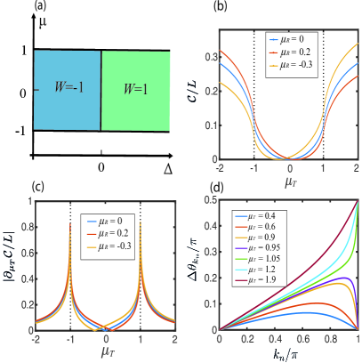
Figure 1: (a) Phase diagram of the Kitaev chain, with $W$ denoting the winding number. (b) Ground state circuit complexity and (c) its derivative versus target state chemical potential ($\mu_{T}$) for several reference states, each with a different chemical potential $\mu_{R}$. (d) Bogoliubov angle difference, $\Delta\theta_{k_{n}}$, for different target ground states, with $\mu_{R}=0$. $\Delta_{R}=\Delta_{T}=1$ for (b)–(d), and $L=1000$ for (b) and (c).

We first choose a fixed ground state as the reference state and calculate the circuit complexities for target ground states with various chemical potentials $\mu_{T}$, crossing the phase transition point. The circuit complexity increases as the difference between the parameters of reference and target states is increased [Fig. 1(b)]. More importantly, the complexity grows rapidly around the critical points ($\mu_{T}=\pm 1$), changing from a convex function to a concave function at the critical points. This is further illustrated in Fig. 1(c), where we plot the derivative (susceptibility) of circuit complexity with respect to $\mu_{T}$ . The clear divergence at the critical points indicates that circuit complexity is nonanalytical at the critical points (see Supplemental Material sup for derivation), and thus can signal the presence of a quantum phase transition. We emphasize that these features are robust signatures of phase transitions, which do not change if one chooses a different reference state in the same phase [see Figs. 1(b) and (c)].

We further plot $\Delta\theta_{k_{n}}$ versus the momentum $k_{n}$, for various target states (with a fixed reference state) in Fig. 1(d). When both states are in the same phase, $\Delta\theta_{k_{n}}$ first increases with momentum, and finally decreases to $0$ when $k_{n}$ approaches $\pi$. In contrast, when $\mu_{T}$ is beyond its critical value, $\Delta\theta_{k_{n}}$ increases monotonically with momentum, and takes the maximal value of $\pi/2$ at $k_{n}=\pi$. This is closely related to the topological phase transition characterized by winding numbers, where the Bogoliubov angles of two different states end up at the same pole (on the Bloch sphere) upon winding half of the Brillouin zone if the states belong to the same phase Alicea (2012). Hence, the non-analytical nature of the circuit complexity is closely related to change of topological number (and topological phase transition).

Analytically, the derivatives of the circuit complexity (7) can be explicitly recast into a closed contour integral over the complex variable $z=e^{ik}$ (see the Supplemental Material sup for detailed derivations). Depending on the parameters of the target states, the poles associated with the integrand are located inside or outside the contour. When the target state goes across a phase transition, the poles sit exactly on the contour, resulting in the divergence of the derivatives of the circuit complexity at critical points sup . Interestingly, the whole parameter space can be classified into four different phase regimes depending on which poles lie inside the contour [see Fig. S1 in Supplemental Material sup ] , which agrees exactly with the phase diagram shown in Fig. 1(a).

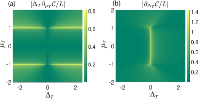
Figure 2: Derivative of circuit complexity as a function of $\mu_{T}$ and $\Delta_{T}$. Panel (a) plots the derivative with respect to $\mu_{T}$ (in units of $1/\Delta_{T}$), and panel (b) plots the derivative with respect to $\Delta_{T}$. The reference state is chosen as the ground state of Eq. (1) with $\mu_{R}=0$ and $\Delta_{R}=-1$, and $L=1000$.

Figures 2(a) and (b) show the derivative of circuit complexity with respect to $\mu_{T}$ and $\Delta_{T}$ for the whole parameter regime. The derivatives show clear singular behavior at both the horizontal [Fig. 2(a)] and vertical [Fig. 2(b)] phase boundaries. Therefore, by using the first-order derivative of complexity with respect to $\mu_{T}$ and $\Delta_{T}$, one can map out the entire equilibrium phase boundaries of the Kitaev chain.

Real-space locality of the optimal Hamiltonian.— Since the ground state [Eq. (3)] is a product of all momentum pairs, the optimal circuit connecting two different ground states corresponds to the following Hamiltonian:

$$\hat{H}_{c}=\sum_{k>0}\hat{H}_{k}=\sum_{k>0}-i\Delta\theta(k)\hat{\psi}_{k}^{\dagger}\tau_{1}\hat{\psi}_{k}^{\phantom{\dagger}},$$ (10)

where $\tau_{i}$ are the Pauli matrices, and $\hat{\psi}_{k}$ denotes the Nambu spinor $\hat{\psi}_{k}=\left(\begin{array}[]{c}\hat{a}_{k}\\ \hat{a}_{-k}^{\dagger}\\ \end{array}\right).$ By taking a Fourier series of the above optimal Hamiltonian, one can show that the Hamiltonian can be written in real space (see Supplemental Material for details sup ):

$$\hat{H}_{c}=\sum_{j}\sum_{n=1}^{\infty}\omega_{n}\left(\hat{a}_{j}\hat{a}_{j+n}-\textrm{H.c.}\right),$$ (11)

where ${\Delta\theta(k)}=2\sum_{n=1}^{\infty}\omega_{n}\sin(nk)$.

One crucial observation is that when the two ground states are in the same phase, $\Delta\theta(0)=\Delta\theta(\pi)=0$ [see Fig. 1(d)]; hence the Fourier series of ${\Delta\theta(k)}$ converges uniformly. Therefore, the full series can be approximated by a finite order $N^{*}$ with arbitrarily small error. This immediately implies that the real-space optimal Hamiltonian (11) is local, with a finite range $N^{*}$. In sharp contrast, if the two states belong to different phases, $\Delta\theta(\pi)=\pi/2\neq\Delta\theta(0)=0$; the Fourier series of $\Delta\theta(k)$ converges at most pointwise. Thus the optimal Hamiltonian must be truly long-range (non-local) in real-space sup , given that the total evolution time is chosen to be a constant [Eq. (5)]. Comparing to previous works on classifying gapped phases of matter using local unitary circuits Bravyi et al. (2006); Chen et al. (2010); Huang and Chen (2015), our results provide an alternative approach that has a natural geometric interpretation.

Complexity for dynamical topological phase transition.—Dynamical phase transitions have received tremendous interest recently Heyl and Budich (2017); D’Alessio and Rigol (2015); Caio et al. (2015); Vajna and Dóra (2015); Wilson et al. (2016); Wang et al. (2017); Caio et al. ; Heyl et al. (2018); Roy et al. (2017); Titum et al. ; Zhang et al. (2017); Jurcevic et al. (2017); Fläschner et al. (2018). Studies on quench dynamics of circuit complexity have mostly focused on growth rates in the short-time regime Alves and Camilo (2018); Jiang et al. . Here, we show that the long-time steady-state value of the circuit complexity following a quantum quench can be used to detect dynamical topological phase transitions.

We take the initial state to be the ground state of a Hamiltonian $\hat{H}_{i}$, and consider circuit complexity growth under a sudden quench to a different Hamiltonian, $\hat{H}_{f}$. The reference and target states are chosen as the initial state $\ket{\Psi_{i}}$ and time-evolved state $\ket{\Psi(t)}$ respectively. The time-dependent $\ket{\Psi(t)}$ can be written as Quan et al. (2006); Kells et al. (2014)

$$\ket{\Psi(t)}=\prod_{n=0}^{\frac{L}{2}-1}\big{[}\cos(\Delta\theta_{k_{n}})-ie^{2i\varepsilon_{k_{n}}t}\sin(\Delta\theta_{k_{n}})\hat{A}_{k_{n}}^{\dagger}\hat{A}_{-k_{n}}^{\dagger}\big{]}\ket{0},$$ (12)

where $\Delta\theta_{k_{n}}$ is the Bogoliubov angle difference between eigenstates of $\hat{H}_{i}$ and $\hat{H}_{f}$, and $\varepsilon_{k_{n}}$ and $\hat{A}_{k_{n}}$ are the energy levels and normal mode operators, respectively, for the post-quench Hamiltonian. Similar to the previous derivations, one can obtain the time-dependent circuit complexity,

$$\mathcal{C}(\ket{\Psi_{i}}\rightarrow\ket{\Psi(t)})=\sum_{k_{n}}\phi_{k_{n}}^{2}(t)$$ (13)

where $\phi_{k_{n}}(t)=\arccos\sqrt{1-\sin^{2}(2\Delta\theta_{k_{n}})\sin^{2}(\varepsilon_{k_{n}}t)}$.

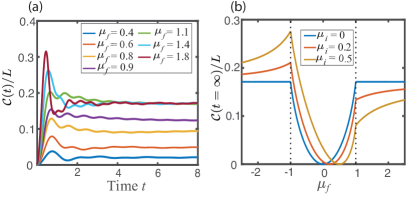
Figure 3: (a) Circuit complexity growth for various post-quench chemical potentials, $\mu_{f}$. The initial state (serves as the reference state) is the ground state of Eq. (1) with $\mu_{i}=0$. (b) Steady-state values of complexity versus $\mu_{f}$. The different lines denote different initial/reference states. $\Delta_{i}=\Delta_{f}=1$ and $L=1000$ in both plots.

As shown in Fig. 3(a), the circuit complexity first increases linearly and then oscillates Camargo et al. ; Alves and Camilo (2018); Jiang et al. before quickly approaching a time-independent value. The steady-state value of circuit complexity increases with $\mu_{f}$ of the post-quench Hamiltonian, until the phase transition occurs [Fig. 3(a)]. Fig. 3(b) further illustrates the long-time steady-state values of circuit complexity versus $\mu_{f}$ for different initial states. The steady-state complexity clearly exhibits nonanalytical behavior at the critical point. This behavior arises because the time-averaged value of $\phi_{k_{n}}(t)$ exhibits an upper bound after the phase transition (see Supplemental Material sup ), and it is a robust feature of the dynamical phase transition regardless of the initial state.

Generalization to long-range Kitaev chain and higher dimensions.—We further give an example of a Kitaev chain with long-range pairing Vodola et al. (2014, 2016); Patrick et al. (2017); Pezzè et al. (2017):

$$\begin{split}\hat{H}_{\text{LR}}=&-\frac{J}{2}\sum_{j=1}^{L}(\hat{a}_{j}^{\dagger}\hat{a}^{\phantom{\dagger}}_{j+1}+\mathrm{H.c.})-\mu\sum_{j=1}^{L}(\hat{a}_{j}^{\dagger}\hat{a}^{\phantom{\dagger}}_{j}-\frac{1}{2})\\ &+\frac{\Delta}{2}\sum_{j=1}^{L}\sum_{\ell=1}^{L-1}\frac{1}{d_{\ell}^{\alpha}}(\hat{a}_{j}^{\dagger}\hat{a}_{j+\ell}^{\dagger}+\mathrm{H.c.}),\end{split}$$ (14)

where $d_{\ell}=\min(\ell,L-\ell)$. In contrast to the short-range model, the long-range model with $\alpha<1$ hosts topological phases with semi-integer winding numbers Vodola et al. (2014); Pezzè et al. (2017).

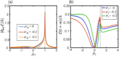
Figure 4: (a) Derivative of circuit complexity with respect to $\mu_{T}$ for three different reference ground states of the long-range Kitaev chain, with $\Delta_{R}=\Delta_{T}=1.3$. (b) Steady-state value of circuit complexity versus $\mu_{f}$ for three different initial ground states, with $\Delta_{i}=\Delta_{f}=1$. $L=1000$ and $\alpha=0$ in both plots.

As one can see, the derivative of ground state circuit complexity only diverges at $\mu_{T}=1$ [Fig. 4(a)], in contrast with Fig. 1(c). This agrees perfectly with the phase diagram for the long-range interacting model, where a topological phase transition occurs only at $\mu=1$ for $\alpha=0$ Pezzè et al. (2017). Figure 4(b) shows the long-time steady-state values of the circuit complexity after a sudden quench. Again, one observes nonanalytical behavior only at $\mu_{T}=1$.

While we have so far restricted ourselves to 1D, the results we found can be readily generalized to higher dimensions Xiong et al. , for example, to $p+ip$ topological superconductors in 2D. The ground state wavefunction of a $p+ip$ superconductor essentially takes the same form as Eq. (3), with the momenta now being restricted to the 2D Brillouin zone, and ${\tan}(2\theta_{\bm{k}})=|\Delta_{\bm{k}}|/\varepsilon_{\bm{k}}$, where $\Delta_{k}$ and $\varepsilon_{\bm{k}}$ denote pairing and kinetic terms in 2D. The circuit complexity can still be written as $\mathcal{C}=\sum_{\bm{k}}|\Delta\theta_{\bm{k}}|^{2}=\frac{L^{2}}{(2\pi)^{2}}\int{\rm d}^{2}{\bm{k}}|\Delta\theta({\bm{k}})|^{2}$. One can show again that the derivative of the circuit complexity is given by (see Supplemental Material sup )

$$\partial_{\mu_{T}}\mathcal{C}=\frac{L^{2}}{(2\pi)^{2}}\int{\rm d}^{2}{\bm{k}}\frac{\theta^{T}(\bm{k})|\Delta({\bm{k}})|}{E({\bm{k}})^{2}},$$ (15)

where $E({\bm{k}})^{2}=\epsilon({\bm{k}})^{2}+|\Delta({\bm{k}})|^{2}$ and $\theta^{T}({\bm{k}})$ denotes the Bogoliubov angle for the target state. It is thus obvious that non-analyticity happens at the critical point where $E({\bm{k}})=0$ sup .

Conclusions and outlook.—We use Nielsen’s approach to quantify the circuit complexity of ground states and nonequilibrium steady states of the Kitaev chain with short- and long-range pairing. We find that, in both situations, circuit complexity can be used to detect topological phase transitions. The non-analytic behaviors can be generalized to higher-dimensional systems, such as $p+ip$ topological superconductors Hasan and Kane (2010); Qi and Zhang (2011).

One interesting future direction is to use the geometric approach to quantify circuit complexity when the control Hamiltonians are constrained to be local in real-space Hyatt et al. (2017); Girolami (2019); Huang and Chen (2015), and study its connection to quantum phase transitions Vojta (2003); Lieb et al. (1961); Katsura (1962); Perk et al. (1975). It would also be of interest to investigate the circuit complexity of interacting many-body systems. One particular example is the XXZ spin-half chain, whose low-energy physics can be modeled by the Luttinger liquid Haldane (1981); Voit (1995); Rahmani and Chamon (2011). By restricting to certain classes of gates (i.e., by imposing penalties on the cost function) Nielsen ; Jefferson and Myers (2017), it might be possible to find improved methods to efficiently prepare the ground state of the XXZ model by calculating the geodesic path in gate space.

Note added: While finalizing this manuscript, we became aware of Ref. Ali et al. , which used revivals in the circuit complexity as a qualitative probe of phase transitions in the Su-Schrieffer-Heeger model. In contrast to that work, we have shown that the circuit complexity explicitly exhibits nonanalyticities precisely at the critical points for the Kitaev chain. We also became aware of Ref. Xiong et al. , which numerically studied the complexity of a two- dimensional “ ${\textbf{d}}\cdot\tau$” model. By contrast, here we analytically study the “$p+ip$” model, and illustrate that the closing of the gap is essential for the nonanalyticity of circuit complexity.

Supplemental Material

This Supplemental Material consists of four sections. In Sec. I, we analytically derive the circuit complexity for a pair of fermions [Eq. (7) of the main text]. In Sec. II, we provide detailed derivations of the nonanalyticity of circuit complexity, as shown numerically in Figs. 1(b) and (c) and Figs. 2(a) and (b) of the main text. In Sec. III, we discuss the real-space structure of the optimal circuit. In Sec. IV, we provide numerical and analytical evidence of the nonanalyticity of steady-state circuit complexity after a quantum quench. Finally, in Sec. V, we provide a detailed analysis of circuit complexity for $p+ip$ topological superconductor.

I Derivation of circuit complexity for a pair of fermions

In this section, we present a detailed derivation of the circuit complexity for a pair of fermions, i.e. Eq. (7) in the main text. This expression has previously been obtained using different approaches in Refs. Hackl and Myers (2018); Khan et al. ; Reynolds and Ross (2018). In order to be comprehensive, here we provide a detailed derivation following Ref. Khan et al. . We note that Ref. Hackl and Myers (2018) provides an alternative derivation using a group theory approach.

By taking the derivative with respect to $s$ in Eq. (5) of the main text, we get the following expression:

$$\sum_{I}Y^{I}(s)O_{I}=(\partial_{s}U(s))U^{-1}(s),$$ (S1)

where $U(s)$ is a unitary transformation which depends on $s$, and we have omitted the label $k$ for notational clarity.

The unitary $U(s)$ can be parametrized in matrix form:

$$U(s)=e^{i\beta}\begin{bmatrix}e^{-i\phi_{1}}\cos{\omega}&\ \ e^{-i\phi_{2}}\sin{\omega}\\ -e^{i\phi_{2}}\sin{\omega}&\ \ e^{i\phi_{1}}\cos{\omega}\end{bmatrix},$$ (S2)

where $\beta,\phi_{1},\phi_{2},\omega$ explicitly depend on the parameter $s$. The above matrix can be expressed in terms of the generators of $U(2)$, which we choose as follows:

$$O_{0}=\begin{bmatrix}i&0\\ 0&i\end{bmatrix},\\ O_{1}=\begin{bmatrix}0&i\\ i&0\end{bmatrix},\\ O_{2}=\begin{bmatrix}0&1\\ -1&0\end{bmatrix},\\ O_{3}=\begin{bmatrix}i&0\\ 0&-i\end{bmatrix}.$$ (S3)

Using the relation

$$\operatorname{tr}(O_{a}O_{b})=-2\delta_{ab},$$ (S4)

one can extract the strength, $Y^{I}(s)$, of generator $O_{I}$ [cf. Eq. 5 in the main text] as follows:

$$Y^{I}(s)=-\frac{1}{2}\operatorname{tr}\left[(\partial_{s}U(s))U^{-1}(s)O_{I}\right].$$ (S5)

Our cost functional can then be expressed as

$$\mathcal{D} = \int_{0}^{1}ds\sum_{I}|Y^{I}(s)|^{2}$$ (S6)

$$= \int_{0}^{1}ds\Bigg{[}\left(\frac{d\beta}{ds}\right)^{2}+\left(\frac{d\omega}{ds}\right)^{2}+\cos^{2}\omega\left(\frac{d\phi_{1}}{ds}\right)^{2}$$

$$\quad\quad\quad\quad+\sin^{2}\omega\left(\frac{d\phi_{2}}{ds}\right)^{2}\Bigg{]}.$$

Now, by exploiting the boundary condition at $s=0$, i.e. $U(s=0)=I$, we get

$$\begin{pmatrix}\beta(s=0)\\ \phi_{1}(s=0)\\ \phi_{2}(s=0)\\ \omega(s=0)\end{pmatrix}=\begin{pmatrix}0\\ 0\\ \phi_{2}(0)\\ 0\end{pmatrix},$$ (S7)

where $\phi_{2}(0)$ is an arbitrary phase. Furthermore, we have the boundary condition at $s=1$,

$$U(s=1)=\begin{bmatrix}\cos(\Delta\theta)&-ie^{-i\phi}\sin(\Delta\theta)\\ -i\sin(\Delta\theta)&e^{-i\phi}\cos(\Delta\theta)\end{bmatrix},$$ (S8)

which results in

$$\begin{pmatrix}\beta(s=1)\\ \phi_{1}(s=1)\\ \phi_{2}(s=1)\\ \omega(s=1)\end{pmatrix}=\begin{pmatrix}0\\ 0\\ \pi/2\\ \Delta\theta\end{pmatrix}.$$ (S9)

The integrand in Eq. (S6) is a sum of four non-negative terms. Setting $\beta(s)=\phi_{1}(s)=0$ and $\phi_{2}(s)=\pi/2$ minimizes (i.e. sets to zero) three of the four terms without imposing any additional constraints on the minimization of the remaining $(d\omega/ds)^{2}$ term. One can then easily check that the linear function $w(s)=s\Delta\theta$ minimizes the remaining term and yields

$$\mathcal{C}=\int_{0}^{1}ds\,|\Delta\theta|^{2}=|\Delta\theta|^{2}.$$ (S10)

II Analytical Derivation of divergent derivatives in ground states

In this section, we provide a detailed analytical derivation to show that the first-order derivative indeed diverges at the critical points in the thermodynamic limit. We first derive how the derivative diverges when the reference state is in the trivial phase ($|\mu_{R}|>1$), and then we generalize our results to show how this divergent behavior depends on the particular choice of the reference state. Throughout this section we assume the reference lies within a given phase, and allow the target state to approach an arbitrary point in the phase diagram. Our analytical derivations show that these divergences necessarily map out the phase boundary, as illustrated in Figs. 2(a) and (b) in the main text and Fig. S1 below.

We begin with our general expression for the complexity as a function of our reference and target states. The Bogoliubov angle difference $\Delta\theta_{k}$ for each momentum sector $k$ can be expressed as

and the circuit complexity is written in terms of $\Delta\theta_{k}$:

$$\mathcal{C}/L=\frac{1}{2\pi}\int_{0}^{\pi}|\Delta\theta_{k}|^{2}\,dk.$$ (S12)

Note that we have replaced the discrete sum in the main text with an integral for the thermodynamic limit, and written “$\mathcal{C}\left(\ket{\Psi_{\text{gs}}^{R}}\rightarrow\ket{\Psi_{\text{gs}}^{T}}\right)$” as “$\mathcal{C}$” for brevity.

Now we substitute Eq. S11 into Eq. S12, and take the derivatives with respect to $\mu_{T}$ and $\Delta_{T}$. We obtain

$$\partial_{\mu_{T}}\mathcal{C}/L = \frac{\Delta_{T}}{4\pi}\int_{-\pi}^{\pi}\frac{\Delta\theta_{k}\sin k}{(\mu_{T}+\cos k)^{2}+\Delta_{T}^{2}\sin^{2}k}\,dk,$$

$$\partial_{\Delta_{T}}\mathcal{C}/L = -\frac{1}{4\pi}\int_{-\pi}^{\pi}\frac{\Delta\theta_{k}\sin k\left(\mu_{T}+\cos k\right)}{(\mu_{T}+\cos k)^{2}+\Delta_{T}^{2}\sin^{2}k}\,dk.\qquad$$ (S13)

Here, we have used the fact that these functions are even in $k$ to extend the integrals to $-\pi$. In spite of the complicated nature of these integrals, much can be learned about their analytic properties by recasting them as closed contour integrals in the complex plane. Defining the variable $z=e^{ik}$, we find that the integrals take the form

$$\partial_{\mu_{T}}\mathcal{C}/L = -i\Delta_{T}\oint\frac{dz}{2\pi i}\frac{\Delta\theta(z)(z^{2}-1)}{(z^{2}+2\mu_{T}z+1)^{2}-\Delta_{T}^{2}(z^{2}-1)^{2}},$$

$$\partial_{\Delta_{T}}\mathcal{C}/L = \frac{i}{2}\oint\frac{dz}{2\pi iz}\frac{\Delta\theta(z)\left(z^{2}-1\right)\left(z^{2}+2\mu_{T}z+1\right)}{(z^{2}+2\mu_{T}z+1)^{2}-\Delta_{T}^{2}(z^{2}-1)^{2}},$$

where the integration is taken counter-clockwise over the contour $|z|=1$. In this form, we may use the fact that the value of the integrals is entirely determined by the non-analyticities of the integrand which are located inside the contour, and that the value of the integration will only diverge if there is a divergence located on the contour.

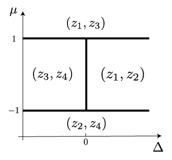
Figure S1: The phase diagram of the Kitaev chain, where in each phase we list which of the two branch points given in Eq. (S15) lie inside the contour integrals in Eq. (LABEL:eq:divC2). The integrals can only diverge at the phase transitions, where the branch points cross the contour,

We proceed by defining the following variables,

$$z_{1,a} = \frac{-\mu_{a}+\sqrt{\mu_{a}^{2}+\Delta_{a}^{2}-1}}{1+\Delta_{a}},$$

$$z_{2,a} = \frac{-\mu_{a}-\sqrt{\mu_{a}^{2}+\Delta_{a}^{2}-1}}{1+\Delta_{a}},$$

$$z_{3,a} = \frac{-\mu_{a}+\sqrt{\mu_{a}^{2}+\Delta_{a}^{2}-1}}{1-\Delta_{a}},$$

$$z_{4,a} = \frac{-\mu_{a}-\sqrt{\mu_{a}^{2}+\Delta_{a}^{2}-1}}{1-\Delta_{a}},$$ (S15)

where $a=R,T$. From Eq. (LABEL:eq:divC2), both derivatives contain simple poles at $z_{i,T}$ for $i=1,2,3,4$, while $\partial_{\Delta_{T}}\mathcal{C}$ additionally has a simple pole at $z=0$. Also, using the formula $\arctan(z)=(i/2)\log\frac{1-iz}{1+iz}$, we can write the Bogoliubov angle as

$$\Delta\theta(z) = \frac{i}{4}\log\Bigg{[}\frac{(\Delta_{T}+1)(z-z_{1,T})(z-z_{2,T})}{(\Delta_{T}-1)(z-z_{3,T})(z-z_{4,T})}$$ (S16)

$$\times\ \frac{(\Delta_{R}-1)(z-z_{3,R})(z-z_{4,R})}{(\Delta_{R}+1)(z-z_{1,R})(z-z_{2,R})}\Bigg{]}.$$

The important fact we will need is that the complex logarithm contains branch cuts running from the zeros to the infinities of its argument; therefore, the $z_{ia}$ are really branch points of the integrand. We now note that the derivatives of the complexity will only diverge if the couplings are tuned to a phase transition. This is because the $z_{i,a}$ can only have unit modulus if we are at one of the phase transitions, and at the phase transitions the branch points cross the contour resulting in a divergent integral, see Fig. S1. In particular, we may characterize the phase diagram in terms of which branch points are inside or outside the contour integral.

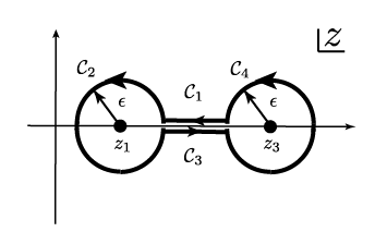
Figure S2: The deformation of the integration contour used to compute the gradients of the circuit complexity in the case $\mu_{T}>1$. There is a branch cut running between the branch points $z_{1}$ and $z_{3}$, where the imaginary part of the integrand is discontinuous and the integrand diverges near the branch points.

In addition, we may actually compute the integrals exactly in certain cases and limits, which allows us to obtain the exact analytic dependence of the divergence on the couplings. As a definite example, we consider the case $|\mu_{T}|>1$. In this case, there is a branch cut inside the logarithm running from $z_{1,T}$ to $z_{3,T}$, and one outside between $z_{2,T}$ and $z_{4,T}$, and the divergences seen at $\mu_{T}\rightarrow 1$ will be due to these branch cuts approaching the contour. In this case we may entirely factor out the dependence on the reference state from the logarithm and focus on the terms which depend on the target state. We deform the contour so that it skirts the branch cut [see the parametrization into four contours in Fig. S2]. A key point here is that the argument of the logarithm is $-\pi$ upon approaching the branch cut from the bottom-half plane, while it is $+\pi$ upon approaching it from the top half. Therefore, in the sum of the two contours running along the branch cut, the logarithm simply contributes a phase factor and we may evaluate the resulting simplified integrand by elementary methods, and for small $\epsilon$ we find

We perform the integral around contour $\mathcal{C}_{2}$ by writing $z=z_{1}+\epsilon e^{i\theta}$, and integrating from $-\pi<\theta<\pi$. At small $\epsilon$, we find

The computation for contour $\mathcal{C}_{4}$ is similar, although the phase winds around the other way:

Finally, taking the sum of all four contours, we find that the $\log\epsilon$ divergence in each integral cancels, and we obtain the desired result:

$$\partial_{\mu_{T}}\mathcal{C}/L = \frac{1}{8\sqrt{\mu_{T}^{2}+\Delta_{T}^{2}-1}}\log\left|\frac{\mu_{T}^{2}-1}{\mu_{T}^{2}+\Delta_{T}^{2}-1}\right|$$ (S20)

$$+\ I_{2}(\mu_{R},\Delta_{R},\mu_{T},\Delta_{T}),$$

where the function $I_{2}$ depends on $\mu_{R}$ and $\Delta_{R}$, but is analytic as the phase transition is approached. Therefore, when approaching from $\mu_{T}>1$, the quantity $\partial_{\mu_{T}}\mathcal{C}/L$ diverges as $\log(\mu_{T}-1)/8\Delta_{T}$ if $\Delta_{T}\neq 0$, but it is analytic if one approaches the multicritical point at $\Delta_{T}=0$.

Similar manipulations may be made for $\partial_{\Delta_{T}}\mathcal{C}/L$ and in other phases. Sometimes the branch cuts take a complicated form in the complex plane so that we cannot reduce the expression into elementary integrals, but we can still deduce the form of the divergence by considering how the contour integrals behave as the branch points cross the contour.

Our final results are summarized as follows. The expression $\partial_{\mu_{T}}\mathcal{C}/L$ is always analytic unless $\mu_{T}\rightarrow\pm 1$. Near these phase transitions, it diverges as

$$\partial_{\mu_{T}}\mathcal{C}/L\sim\frac{\mathrm{sign}(\mu_{T})}{8\sqrt{\mu_{T}^{2}+\Delta_{T}^{2}-1}}\log\left|\frac{\mu_{T}^{2}-1}{\mu_{T}^{2}+\Delta_{T}^{2}-1}\right|,$$ (S21)

so the divergence is $\mathrm{sign}(\mu_{T})\log|\mu_{T}-1|/8\Delta_{T}$ if $\Delta_{T}\neq 0$, but there is not a divergence at $\Delta_{T}=0$.

In contrast, the expression $\partial_{\Delta_{T}}\mathcal{C}/L$ is analytic whenever $\Delta_{T}\neq 0$. In this case, the divergence depends on whether the couplings $(\mu_{T},\Delta_{T})$ approach the phase transitions from the topological phase or the trivial phase. If we approach the multicritical points from the trivial phases, we find that $\partial_{\Delta_{T}}\mathcal{C}/L$ remains analytic. In contrast, if we approach $\Delta_{T}=0$ from the topological phases, we find

$$\partial_{\Delta_{T}}\mathcal{C}/L\sim\frac{1}{4}\left(1+\frac{|\mu_{T}\Delta_{T}|}{\sqrt{|\mu_{T}^{2}+\Delta_{T}^{2}-1|}}\right)\log\left|\Delta_{T}\right|.$$ (S22)

In this case, we have a $\log|\Delta_{T}|/4$ divergence when $|\mu_{T}|<1$, but now we find that the divergence crosses over to $\log|\Delta_{T}|/2$ as we approach the multicritical points.

III Real-space behavior of the optimal circuits

In this section, we show how that the real-space optimal circuit behaves differently depending on whether or not the initial and target states are in the same topological phase.

As we have derived in Sec. I of the Supplemental Material, for a single momentum sector $k$, the circuit complexity is found to be the squared difference between the Bogoliubov angles [Eq. (7) in the main text], and the optimal circuit is generated by the following time-independent Hamiltonian,

$$\mathcal{H}_{k}=-\Delta\theta_{k}\,O_{1,k},$$ (S23)

where $O_{1,k}$ is the same generator given by Eq. (S3) for momentum sector $k$. Here, we have omitted the time label ‘$s$’ for simplicity as the circuit is time independent (and the total evolution time is fixed to be constant 1). As in the main text and following the circuit complexity literature, we have defined $\mathcal{H}_{k}$ to be anti-Hermitian [Eq. 5].

Since the ground state of the Hamiltonian is a product of all momentum sectors with $k>0$, the optimal circuit which generates the evolution between two ground states can be written as

$$\mathcal{H}=\sum_{k>0}\mathcal{H}_{k}=\sum_{k>0}-\Delta\theta_{k}\,O_{1,k}.$$ (S24)

We are interested in the real-space behavior of the above Hamiltonian. To discern this, we first write the above Hamiltonian in operator form

$$\mathcal{H}=\sum_{k>0}\mathcal{H}_{k}=\sum_{k>0}-i\Delta\theta(k)\hat{\psi}_{k}^{\dagger}\tau_{1}\hat{\psi}_{k}^{\phantom{\dagger}},$$ (S25)

where $\tau_{i}$ are the Pauli matrices, and $\hat{\psi}_{k}$ denotes the Nambu spinor

$$\hat{\psi}_{k}=\left(\begin{array}[]{c}\hat{a}_{k}\\ \hat{a}_{-k}^{\dagger}\\ \end{array}\right).$$ (S26)

Utilizing the particle-hole symmetry of the Nambu spinor

$$\hat{\psi}_{-k}=\tau_{1}(\hat{\psi}_{k}^{\dagger})^{T},$$ (S27)

we can extend the sum in the evolution Hamiltonian to be over the entire Brillouin zone

$$\mathcal{H}=\sum_{k}-i\omega(k)\hat{\psi}_{k}^{\dagger}\tau_{1}\hat{\psi}_{k}^{\phantom{\dagger}},$$ (S28)

where $\omega(k)$ satisfies

$$\omega(k)-\omega(-k)=\Delta\theta(k)$$ (S29)

for $k>0$. In particular, only the odd part of the function contributes since the even part cancels in the $\tau_{1}$ pairing channel.

We now proceed by performing a Fourier series expansion of the function $\omega(k)$ over the Brillouin zone. Without loss of generality we may consider only the odd Fourier series since the even terms will cancel. Thus, we write

$$\omega(k)=\sum_{n=1}^{\infty}\omega_{n}\sin(nk)=\frac{\Delta\theta(k)}{2},$$ (S30)

where the last equality is used to determine the Fourier coefficients.

Our crucial observation is that when the two states are within the same phase, the Fourier sine series for $\Delta\theta(k)$ ought to be uniformly convergent. This can be seen by considering the boundary conditions, which in this case read $\Delta\theta(0)=\Delta\theta(\pi)=0$, as shown in Fig. 1(d) in the main text. Thus, if we allow the time-evolved state $\ket{\Psi_{T}^{\prime}}$ to be within an arbitrarily small error $\epsilon$ to the real target state $\ket{\Psi_{T}}$, this Fourier series can be accurately truncated to a finite order $N^{*}$ over the entire Brillouin zone.

This is relevant because in real-space, the Fourier harmonic $\sin(lk)\,\hat{\psi}_{k}^{\dagger}\tau_{1}\hat{\psi}_{k}^{\phantom{\dagger}}$ is generated by a term involving two fermionic operators separated by $l$ sites. More specifically, as this occurs in the $\tau_{1}$ channel, $\mathcal{H}$ must involve real-space pairing terms such that

$$\mathcal{H}=\sum_{j}\sum_{n=1}^{N^{*}}\omega_{n}\left(\hat{a}_{j}\hat{a}_{j+n}-\textrm{H.c.}\right).$$ (S31)

The above argument holds when the system size $L$ is taken to be infinite. In such a case, the finite-range interacting evolution Hamiltonian can be regarded as a truly short-range Hamiltonian, and our results imply that the optimal circuit (with constant time or depth) which evolve states within the same phase region is short-range.

On the other hand, when the two states are in different phases, the boundary conditions $\Delta\theta(\pi)=\pi/2\neq\Delta\theta(0)=0$ obstruct uniform convergence, analogous to the Gibbs phenomenon. In this case, the Fourier sine series may still converge pointwise, but for fixed error the series cannot be truncated to finite order $N^{*}$ over the entire Brillouin zone. In such cases, the optimal evolution Hamiltonian $\mathcal{H}$ that transforms states between different topological phases must be long-range when the evolution time is fixed to be a constant. Again, this is because the longest real-space distance required to generate the evolution Hamiltonian is given by the highest order of Fourier mode appearing in the momentum space series, which now cannot be accurately truncated.

IV Numerical evidence for nonanalyticity of quench dynamics

In this section, we provide detailed numerical explanations for the nonanalyticity of the long-time steady-state value of the circuit complexity at critical points, as observed in Fig. 3(b) of the main text.

As derived in the main text, the time-dependent circuit complexity is given by

$$\mathcal{C}(\ket{\Psi_{i}}\rightarrow\ket{\Psi(t)})=\sum_{k_{n}}\phi_{k_{n}}^{2}(t),$$ (S32)

where

$$\phi_{k_{n}}(t)=\arccos\sqrt{1-\sin^{2}(2\Delta\theta_{k_{n}})\sin^{2}(\varepsilon_{k_{n}}t)}.$$ (S33)

Then the long-time steady-state complexity is just given by the time-averaged value of the above expression,

$$\overline{\mathcal{C}(\ket{\Psi_{i}}\rightarrow\ket{\Psi(t)})}=\sum_{k_{n}}\overline{\phi_{k_{n}}^{2}(t)},$$ (S34)

where the overline denotes time averaging. Because ${\phi_{k_{n}}^{2}(t)}$ is such a complex expression, it is unknown to us how to derive an analytical function for the time-averaged circuit complexity. Instead, we plot ${\overline{\phi_{k_{n}}(t)}}$ numerically, and show that the nonanalyticity indeed occurs at the phase transition.

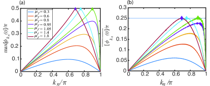
Figure S3: (a) Maximum value of $\phi_{k_{n}}(t)$ versus $k_{n}$ for different post-quench Hamiltonian parameters. (b) Time-averaged value of $\phi_{k_{n}}(t)$ versus $k_{n}$ for different post-quench Hamiltonian parameters. In both panels, $\mu_{i}=0$, $\Delta_{i}=\Delta_{f}=1$, and $L=1000$. The diamond markers denote the expected locations of the maxima across the phase transition, given by solutions to $1+\mu_{f}\cos{k_{n}}=0$ (see text).

From the expression of $\phi_{k_{n}}(t)$, it is clear that its value oscillates with time, and it reaches its maximal value (envelope) for each momentum sector $k_{n}$ when $\sin(\epsilon_{k_{n}}t)=1$. In Fig. S3(a), we plot the maximum value of $\phi_{k_{n}}(t)$ for different post-quench Hamiltonian parameters. As the figure clearly shows, when the chemical potential $\mu_{f}$ of the post-quench Hamiltonian is below the critical value ($\mu_{f}=1$), $\max[\phi_{k_{n}}(t)]$ is a smooth function of $k_{n}$. However, when $\mu_{f}$ is above the critical value, $\max[\phi_{k_{n}}(t)]$ exhibits a kink at a certain momentum $k_{n}$, with its maximal value reaching $\frac{\pi}{2}$. To understand this behavior, we can write down the expression for $\max[\phi_{k_{n}}(t)]$ given the choice of parameters $\mu_{i}=0,\Delta_{i}=\Delta_{f}=1$:

$$\max[\phi_{k_{n}}(t)]=\arccos{\left|\frac{1+\mu_{f}\cos{k_{n}}}{\sqrt{\mu_{f}^{2}+2\mu_{f}\cos{k_{n}}+1}}\right|}.$$ (S35)

From the above expression, it is clear that when $\mu_{f}<1$, $\max[\phi_{k_{n}}(t)]$ is always smaller than $\pi/2$; when $\mu_{f}>1$, $\max[\phi_{k_{n}}(t)]$ can obtain the maximal value of $\pi/2$ when $1+\mu_{f}\cos{k_{n}}=0$. Because one needs to take the absolute value for the arguments of $\arccos$, the quantity $\max[\phi_{k_{n}}(t)]$ exhibits a kink when reaching $\pi/2$, in agreement with Fig. S3(a).

We plot the time-averaged value of $\phi_{k_{n}}(t)$ in Fig. S3(b). Again, we see an upper bound of $\overline{\phi_{k_{n}}(t)}$ when quenching across the critical point. Similar to Fig. S3(a), $\overline{\phi_{k_{n}}(t)}$ reaches its maximal value when $1+\mu_{f}\cos{k_{n}}=0$, i.e. when $\sin(2\Delta\theta_{k_{n}})=1$. For this special momentum sector, the expression for $\phi_{k_{n}}(t)$ can be written as

$$\phi_{k_{n}}(t)=\arcsin{\left|\sin(\varepsilon_{k_{n}}t)\right|}.$$ (S36)

Clearly, the time-averaged value of the above expression is just $\pi/4$, in agreement with the numerical results shown in Fig. S3(b). Therefore, after the phase transition takes place, the maximal value of $\overline{\phi_{k_{n}}(t)}$ is bounded by $\pi/4$. (This feature is independent of the parameters of the pre-quench Hamiltonian.)

Having revealed this feature of $\overline{\phi_{k_{n}}(t)}$, the nonanalyticity can be understood as follows: as $\mu_{f}$ increases but is still below the phase transition point, the integral of $\overline{\phi_{k_{n}}^{2}(t)}$ increases smoothly with $\mu_{f}$. After reaching the phase transition, $\overline{\phi_{k_{n}}^{2}(t)}$ saturates the bound, and thus the integral’s (circuit complexity’s) dependence on $\mu_{f}$ takes a different form. In particular, for the parameters shown in Fig. S3 [blue line in Fig. 3(b) in the main text], the integral (i.e., the circuit complexity) becomes a constant after the phase transition. This leads to a clear nonanalytical (kink) point at $\mu_{f}=1$.

V Circuit complexity for two-dimensional $p+ip$ topological superconductors

In this section, we show how our results for the 1D Kitaev chain can be generalized to 2D. In particular, we consider a $p+ip$ topological superconductor for which the Hamiltonian can be written in momentum space as:

$$\hat{H}=\sum_{\bm{k}}\hat{\psi}_{\bm{k}}^{\dagger}\mathcal{H}_{\bm{k}}\hat{\psi}_{\bm{k}},$$ (S37)

where the summation is taken over the 2D Brillouin zone, and $\hat{\psi}_{k}=\left(\begin{array}[]{c}\hat{a}_{k}\\ \hat{a}_{-k}^{\dagger}\\ \end{array}\right)$ is the Nambu spinor. The single-particle Hamiltonian takes the following form:

$$\mathcal{H}_{\bm{k}}=\begin{pmatrix}\varepsilon_{\bm{k}}&\Delta_{\bm{k}}^{*}\\ \Delta_{\bm{k}}&-\varepsilon_{\bm{k}}\end{pmatrix},$$ (S38)

where $\varepsilon_{\bm{k}}$ and $\Delta_{\bm{k}}$ denote the kinetic and pairing terms in 2D respectively. The ground state wavefunction can be written as

$$\ket{\Psi_{\text{gs}}}=\prod_{\bm{k}}(\cos\theta_{\bm{k}}-i\sin\theta_{\bm{k}}\hat{a}_{\bm{k}}^{\dagger}\hat{a}_{-\bm{k}}^{\dagger})\ket{0},$$ (S39)

where ${\tan}(2\theta_{\bm{k}})=|\Delta_{\bm{k}}|/\varepsilon_{\bm{k}}$. Similar to 1D, the circuit complexity of the full wavefunction is given by

$$\mathcal{C}=\sum_{\bm{k}}|\Delta\theta_{\bm{k}}|^{2}=\frac{L^{2}}{(2\pi)^{2}}\int{\rm d}^{2}{\bm{k}}|\Delta\theta({\bm{k}})|^{2},$$ (S40)

where we have replaced the summmation by an integral in the infinite-system limit. In this continuum limit, $\varepsilon({\bm{k}})\approx\frac{k^{2}}{2m}-\mu$ and $\Delta({\bm{k}})\approx i\Delta(k_{x}+ik_{y})$.

We expect that the non-analyticity should not depend on the particular choice of initial reference state, so we take $\mu_{R}\rightarrow-\infty$ [with $\theta^{R}({\bm{k}})=0$] for simplicity. This corresponds to the trivial vacuum with no particle. Upon tuning $\mu$, the system undergoes a quantum phase transition into the topological phase at $\mu=0$. Taking the derivative of $\mathcal{C}$ with respect to $\mu_{T}$, we obtain

$$\partial_{\mu_{T}}\mathcal{C} = \frac{L^{2}}{(2\pi)^{2}}\int{\rm d}^{2}{\bm{k}}\ 2\theta^{T}({\bm{k}})\partial_{\mu_{T}}\theta^{T}({\bm{k}})$$ (S41)

$$= \frac{L^{2}}{(2\pi)^{2}}\int{\rm d}^{2}{\bm{k}}\theta^{T}({\bm{k}})\partial_{\mu_{T}}\left[{\arctan}\frac{|\Delta({\bm{k}})|}{\varepsilon({\bm{k}})}\right]$$

$$= \frac{L^{2}}{(2\pi)^{2}}\int{\rm d}^{2}{\bm{k}}\frac{\theta^{T}({\bm{k}})|\Delta({\bm{k}})|}{E({\bm{k}})^{2}}.$$

References

- Watrous (2009) J. Watrous, “Quantum computational complexity,” in Encyclopedia of Complexity and Systems Science, edited by Robert A. Meyers (Springer New York, New York, NY, 2009) pp. 7174–7201.
- (2) S. Aaronson, “The Complexity of Quantum States and Transformations: From Quantum Money to Black Holes,” arXiv:1607.05256 .
- (3) M. A. Nielsen, “A geometric approach to quantum circuit lower bounds,” arXiv:quant-ph/0502070 .
- Nielsen et al. (2006) M. A. Nielsen, M. R. Dowling, M. Gu, and A. C. Doherty, “Quantum Computation as Geometry,” Science 311, 1133 (2006).
- (5) M. R. Dowling and M. A. Nielsen, “The geometry of quantum computation,” arXiv:quant-ph/0701004 .
- Jefferson and Myers (2017) R. A. Jefferson and R. C. Myers, “Circuit complexity in quantum field theory,” J. High Energy Phys. 10, 107 (2017).
- Yang (2018) R.-Q. Yang, “Complexity for quantum field theory states and applications to thermofield double states,” Phys. Rev. D 97, 066004 (2018).
- Guo et al. (2018) M. Guo, J. Hernandez, R. C. Myers, and S.-M. Ruan, “Circuit complexity for coherent states,” J. High Energy Phys. 10, 11 (2018).
- (9) H. A. Camargo, P. Caputa, D. Das, M. P. Heller, and R. Jefferson, “Complexity as a novel probe of quantum quenches: universal scalings and purifications,” arXiv:1807.07075 .
- Alves and Camilo (2018) D. W. F. Alves and G. Camilo, “Evolution of complexity following a quantum quench in free field theory,” J. High Energy Phys. 6, 29 (2018).
- (11) S. Chapman, J. Eisert, L. Hackl, M. P. Heller, R. Jefferson, H. Marrochio, and R. C. Myers, “Complexity and entanglement for thermofield double states,” arXiv:1810.05151 .
- Hackl and Myers (2018) L. Hackl and R. C. Myers, “Circuit complexity for free fermions,” J. High Energy Phys. 7, 139 (2018).
- (13) R. Khan, C. Krishnan, and S. Sharma, “Circuit Complexity in Fermionic Field Theory,” arXiv:1801.07620 .
- Reynolds and Ross (2018) A. P. Reynolds and S. F. Ross, “Complexity of the AdS soliton,” Class. Quantum Grav 35, 095006 (2018).
- (15) J. Jiang, J. Shan, and J. Yang, “Circuit complexity for free Fermion with a mass quench,” arXiv:1810.00537 .
- Yang et al. (2019a) R. Q. Yang, Y. S. An, C. Niu, C. Y. Zhang, and K. Y. Kim, “Principles and symmetries of complexity in quantum field theory,” Eur. Phys. J. C 79, 109 (2019a).
- Yang et al. (2019b) R. Q. Yang, Y. S. An, C. Niu, C. Y. Zhang, and K. Y. Kim, “More on complexity of operators in quantum field theory,” J. High Energy Phys. 2019, 161 (2019b).
- Yang and Kim (2019) R. Q. Yang and K. Y. Kim, “Complexity of operators generated by quantum mechanical Hamiltonians,” J. High Energy Phys. 2019, 10 (2019).
- Stanford and Susskind (2014) D. Stanford and L. Susskind, “Complexity and shock wave geometries,” Phys. Rev. D 90, 126007 (2014).
- (20) L. Susskind, “Computational Complexity and Black Hole Horizons,” arXiv:1402.5674 .
- (21) A. R. Brown, D. A. Roberts, L. Susskind, B. Swingle, and Y. Zhao, “Complexity Equals Action,” arXiv:1509.07876 .
- Brown et al. (2016) A. R. Brown, D. A. Roberts, L. Susskind, B. Swingle, and Y. Zhao, “Complexity, action, and black holes,” Phys. Rev. D 93, 086006 (2016).
- Chapman et al. (2018) S. Chapman, M. P. Heller, H. Marrochio, and F. Pastawski, “Toward a Definition of Complexity for Quantum Field Theory States,” Phys. Rev. Lett 120, 121602 (2018).
- (24) P. Caputa and J. M. Magan, “Quantum Computation as Gravity,” arXiv:1807.04422 .
- Vojta (2003) M. Vojta, “Quantum phase transitions,” Rep. Prog. Phys 66, 2069 (2003).
- Caneva et al. (2007) T. Caneva, R. Fazio, and G. E. Santoro, “Adiabatic quantum dynamics of a random Ising chain across its quantum critical point,” Phys. Rev. B 76, 144427 (2007).
- Sørensen et al. (2010) A. S. Sørensen, E. Altman, M. Gullans, J. V. Porto, M. D. Lukin, and E. Demler, “Adiabatic preparation of many-body states in optical lattices,” Phys. Rev. A 81, 061603 (2010).
- Kitaev (2001) A. Y. Kitaev, “Unpaired Majorana fermions in quantum wires,” Phys.-Uspekhi 44, 131 (2001).
- Alicea (2012) J. Alicea, “New directions in the pursuit of Majorana fermions in solid state systems,” Rep. Prog. Phys 75, 076501 (2012).
- Alicea et al. (2011) J. Alicea, Y. Oreg, G. Refael, F. von Oppen, and M. P. A. Fisher, “Non-Abelian statistics and topological quantum information processing in 1D wire networks,” Nat. Phys 7, 412 (2011).
- Sau et al. (2010) J. D. Sau, R. M. Lutchyn, S. Tewari, and S. Das Sarma, “Generic new platform for topological quantum computation using semiconductor heterostructures,” Phys. Rev. Lett. 104, 040502 (2010).
- Oreg et al. (2010) Y. Oreg, G. Refael, and F. von Oppen, “Helical Liquids and Majorana Bound States in Quantum Wires,” Phys. Rev. Lett. 105, 177002 (2010).
- Lutchyn et al. (2010) R. M. Lutchyn, J. D. Sau, and S. Das Sarma, “Majorana fermions and a topological phase transition in semiconductor-superconductor heterostructures,” Phys. Rev. Lett. 105, 077001 (2010).
- (34) See Supplemental Material for derivations of circuit complexity for a pair of fermions, derivations of the nonanalyticity of circuit complexity at critical points, details of real-space behavior of optimal control Hamiltonians, numerics for the nonanalyticity of circuit complexity after quantum quenches, and circuit complexity for 2D topological superconductors.
- Note (1) In such a space, each state is represented by one point, with its coordinates labeled by the Bogoliubov angles, i.e. .
- Bravyi et al. (2006) S. Bravyi, M. B. Hastings, and F. Verstraete, “Lieb-robinson bounds and the generation of correlations and topological quantum order,” Phys. Rev. Lett. 97, 050401 (2006).
- Chen et al. (2010) X. Chen, Z.-C. Gu, and X.-G. Wen, “Local unitary transformation, long-range quantum entanglement, wave function renormalization, and topological order,” Phys. Rev. B 82, 155138 (2010).
- Huang and Chen (2015) Y. Huang and X. Chen, “Quantum circuit complexity of one-dimensional topological phases,” Phys. Rev. B 91, 195143 (2015).
- Heyl and Budich (2017) M. Heyl and J. C. Budich, “Dynamical topological quantum phase transitions for mixed states,” Phys. Rev. B 96, 180304 (2017).
- D’Alessio and Rigol (2015) L. D’Alessio and M. Rigol, “Dynamical preparation of Floquet Chern insulators,” Nat. Commun 6, 8336 (2015).
- Caio et al. (2015) M. D. Caio, N. R. Cooper, and M. J. Bhaseen, “Quantum Quenches in Chern Insulators,” Phys. Rev. Lett. 115, 236403 (2015).
- Vajna and Dóra (2015) S. Vajna and B. Dóra, “Topological classification of dynamical phase transitions,” Phys. Rev. B 91, 155127 (2015).
- Wilson et al. (2016) J. H. Wilson, J. C. W. Song, and G. Refael, “Remnant Geometric Hall Response in a Quantum Quench,” Phys. Rev. Lett 117, 235302 (2016).
- Wang et al. (2017) C. Wang, P. Zhang, X. Chen, J. Yu, and H. Zhai, “Scheme to Measure the Topological Number of a Chern Insulator from Quench Dynamics,” Phys. Rev. Lett. 118, 185701 (2017).
- (45) M. D. Caio, G. Möller, N. R. Cooper, and M. J. Bhaseen, “Topological Marker Currents in Chern Insulators,” arXiv:1808.10463 .
- Heyl et al. (2018) M. Heyl, F. Pollmann, and B. Dóra, “Detecting Equilibrium and Dynamical Quantum Phase Transitions in Ising Chains via Out-of-Time-Ordered Correlators,” Phys. Rev. Lett. 121, 016801 (2018).
- Roy et al. (2017) S. Roy, R. Moessner, and A. Das, “Locating topological phase transitions using nonequilibrium signatures in local bulk observables,” Phys. Rev. B 95, 041105 (2017).
- (48) P. Titum, J. T. Iosue, J. R. Garrison, A. V. Gorshkov, and Z.-X. Gong, “Probing ground-state phase transitions through quench dynamics,” arXiv:1809.06377 .
- Zhang et al. (2017) J. Zhang, G. Pagano, P. W. Hess, A. Kyprianidis, P. Becker, H. Kaplan, A. V. Gorshkov, Z. X. Gong, and C. Monroe, “Observation of a many-body dynamical phase transition with a 53-qubit quantum simulator,” Nature 551, 601–604 (2017).
- Jurcevic et al. (2017) P. Jurcevic, H. Shen, P. Hauke, C. Maier, T. Brydges, C. Hempel, B. P. Lanyon, M. Heyl, R. Blatt, and C. F. Roos, “Direct Observation of Dynamical Quantum Phase Transitions in an Interacting Many-Body System,” Phys. Rev. Lett. 119, 080501 (2017).
- Fläschner et al. (2018) N. Fläschner, D. Vogel, M. Tarnowski, B. S. Rem, D.-S. Lühmann, M. Heyl, J.C. Budich, L. Mathey, K. Sengstock, and C. Weitenberg, “Observation of dynamical vortices after quenches in a system with topology,” Nat. Phys 14, 265 (2018).
- Quan et al. (2006) H. T. Quan, Z. Song, X. F. Liu, P. Zanardi, and C. P. Sun, “Decay of Loschmidt Echo Enhanced by Quantum Criticality,” Phys. Rev. Lett. 96, 140604 (2006).
- Kells et al. (2014) G. Kells, D. Sen, J. K. Slingerland, and S. Vishveshwara, “Topological blocking in quantum quench dynamics,” Phys. Rev. B 89, 235130 (2014).
- Vodola et al. (2014) D. Vodola, L. Lepori, E. Ercolessi, A. V. Gorshkov, and G. Pupillo, “Kitaev Chains with Long-Range Pairing,” Phys. Rev. Lett 113, 156402 (2014).
- Vodola et al. (2016) D. Vodola, L. Lepori, E. Ercolessi, and G. Pupillo, “Long-range Ising and Kitaev models: phases, correlations and edge modes,” New J. Phys 18, 015001 (2016).
- Patrick et al. (2017) K. Patrick, T. Neupert, and J. K. Pachos, “Topological Quantum Liquids with Long-Range Couplings,” Phys. Rev. Lett 118, 267002 (2017).
- Pezzè et al. (2017) L. Pezzè, M. Gabbrielli, L. Lepori, and A. Smerzi, “Multipartite entanglement in topological quantum phases,” Phys. Rev. Lett. 119, 250401 (2017).
- (58) Z. Xiong, D.-X. Yao, and Z. Yan, “Nonanalyticity of circuit complexity across topological phase transitions,” arXiv:1906.11279 .
- Hasan and Kane (2010) M. Z. Hasan and C. L. Kane, “Colloquium: Topological insulators,” Rev. Mod. Phys. 82, 3045 (2010).
- Qi and Zhang (2011) X.-L. Qi and S.-C. Zhang, “Topological insulators and superconductors,” Rev. Mod. Phys. 83, 1057 (2011).
- Hyatt et al. (2017) K. Hyatt, J. R. Garrison, and B. Bauer, “Extracting entanglement geometry from quantum states,” Phys. Rev. Lett. 119, 140502 (2017).
- Girolami (2019) D. Girolami, “How difficult is it to prepare a quantum state?” Phys. Rev. Lett. 122, 010505 (2019).
- Lieb et al. (1961) E. Lieb, T. Schultz, and D. Mattis, “Two soluble models of an antiferromagnetic chain,” Ann. Phys. 16, 407 (1961).
- Katsura (1962) S. Katsura, “Statistical Mechanics of the Anisotropic Linear Heisenberg Model,” Phys. Rev. 127, 1508 (1962).
- Perk et al. (1975) J. H. H. Perk, H. W. Capel, M. J. Zuilhof, and Th. J. Siskens, “On a soluble model of an antiferromagnetic chain with alternating interactions and magnetic moments,” Physica A 81, 319 (1975).
- Haldane (1981) F. D. M. Haldane, “‘Luttinger liquid theory’of one-dimensional quantum fluids. I. Properties of the Luttinger model and their extension to the general 1D interacting spinless Fermi gas,” J. Phys. Condens. Matter 14, 2585 (1981).
- Voit (1995) J. Voit, “One-dimensional Fermi liquids,” Rep. Prog. Phys 58, 977 (1995).
- Rahmani and Chamon (2011) A. Rahmani and C. Chamon, “Optimal Control for Unitary Preparation of Many-Body States: Application to Luttinger Liquids,” Phys. Rev. Lett. 107, 016402 (2011).
- (69) T. Ali, A. Bhattacharyya, S. Shajidul Haque, E. H. Kim, and N. Moynihan, “Post-Quench Evolution of Distance and Uncertainty in a Topological System: Complexity, Entanglement and Revivals,” arXiv:1811.05985 .