Non-equilibrium Ionization in Mixed-morphology Supernova Remnants

Abstract

The mixed morphology class of supernova remnants (MMSNRs) comprises a substantial fraction of observed remnants and yet there is as yet no consensus on their origin. A clue to their nature is the presence of regions that show X-ray evidence of recombining plasmas. Recent calculations of remnant evolution in a cloudy interstellar medium (ISM) that included thermal conduction but not non-equilibrium ionization (NEI) showed promise in explaining observed surface brightness distributions but could not determine if recombining plasmas were present. In this paper we present numerical hydrodynamical models of MMSNRs in 2D and 3D including explicit calculation of NEI effects. Both the spatial ionization distribution and temperature-density diagrams show that recombination occurs inside the simulated MMSNR, and that both adiabatic expansion and thermal conduction cause recombination, albeit in different regions. Features created by the adiabatic expansion stand out in the spatial and temperature-density diagrams, but thermal conduction also plays a role. Thus thermal conduction and adiabatic expansion both contribute significantly to the cooling of high temperature gas. Realistic observational data are simulated with both spatial and spectral input from various regions. We also discuss the possibility of analyzing the sources of recombination and dominant hydrodynamical processes in observations using temperature-density diagrams and spatial maps.

1 Introduction

Mixed-morphology supernova remnants (MMSNRs) are a class of SNR characterized by Rho & Petre (1998), who defined them as containing a radio shell with centrally brightened thermal X-ray emission. This class is also known as thermal composite SNRs, named by Jones et al. 1998. The external radio shell is believed to be associated with the blastwave shock propagating into the interstellar medium (ISM), but the bright thermal X-ray interior is hard to explain. MMSNRs are usually highly absorbed and almost always found in regions with molecular clouds (MCs). Observational evidence has confirmed that about half out of known 37 MMSNRs are interacted with MCs (Zhang et al., 2015). Given the complex environments the SNRs are evolving in, there have been several possible mechanisms proposed for the brightness of the thermal X-ray interior, such as a radiatively cooled rim (Harrus et al., 1997; Rho & Petre, 1998), thermal conduction in the interior hot gas (Cox et al., 1999; Shelton et al., 1999), evaporation of gas from the shock-engulfed cloudlets (White & Long, 1991), shock reflection (Chen et al., 2008; Zhang et al., 2015), and even projection effects for some particular SNRs (Petruk, 2001; Zhou et al., 2016). Slavin et al. (2017) investigated the influence of a cloudy surrounding medium on the evolution of SNRs with numerical hydrodynamical simulations that included thermal conduction. The results agree with those of White & Long (1991) in that centrally brightened thermal emission is generated, though emission from shocked clouds, which was not included by White & Long (1991), was found to be important. A limitation of the calculations in Slavin et al. (2017) was that the plasma was assumed to be in collisional ionization equilibrium (CIE).

While it has long been known that shocks should produce plasma that is far from CIE and under-ionized for its temperature, it was surprising that some MMSNRs (about 12 out of 37) were found to contain over-ionized (recombining) plasma (See Suzuki et al., 2018, and the references therein). Considering the modest effective area and the spectral resolution of currently available X-ray observatories our ability to diagnose such over-ionization is limited and so the fraction of such remnants could be larger. So far all SNRs found to have recombining plasma belong to the class of MMSNRs, implying a possible correlation between the mechanisms for the overionization and the centrally peaked thermal emission.

In the standard Sedov-Taylor evolution of an SNR in a homogeneous ISM, material is heated by the shock and cools slowly and adiabatically because of expansion of the remnant. Thus to get a significant signature of recombination, some additional cooling mechanisms must be at work. Thermal conduction presents one possible cause of this cooling since when it is operating freely, the hot central region of the remnant cools by conducting its heat to the cooler regions closer to the shock front, leading to flattening of the central temperature profile. Zhou et al. (2011) performed the first hydrodynamical simulation including a shock interacting a ring-like cloud in 2D to investigate the over-ionization seen in a particular SNR, W49B, albeit without considering other cloud configurations or comparing other cooling sources in detail. Other possibilities have also been proposed, such as the transfer of energy from the thermal plasma to cosmic rays (Suzuki et al., 2018) to explain the unexpected ionization. In this paper, we explore the ionization effects of a cloudy ISM on SNR evolution, utilizing hydrodynamic simulations that include thermal conduction and non-equilibrium ionization.

2 Methods and models

To study the effects of thermal conduction and the cloudiness of the ISM on the ionization inside evolving SNRs we performed hydrodynamical simulations using the FLASH code v4.3 (Fryxell et al., 2000). We used the same initialization as runs in Slavin et al. (2017) including using 2D cylindrical symmetry (except as noted below). The new aspect of this study is the use of non-equilibrium ionization (NEI), which utilizes the new NEI unit developed by Zhang et al. (2018). That unit evolves the ionization simultaneously with the hydrodynamics. The gas is assumed to be initially in CIE in the ambient medium at a temperature $T=10^{4}\,{\rm K}$ and a number density $n_{\rm H}=0.25\,{\rm cm}^{-3}$. We do not include the effects of the magnetic field, radiative cooling or energy loss by cosmic ray acceleration in the simulations presented in this paper.

We use the Diffuse module of FLASH code for thermal conduction in the simulation. Both classical Spitzer conductivity (Spitzer, 1956), $\kappa\propto T^{5/2}$, and saturated conductivity (McKee & Cowie, 1977), $\kappa\propto\rho c^{3}$ are supported with a smooth transition from classical to saturated. (see the Appendix in Slavin et al. 2017 for details). For the sake of comparison, we performed three different simulations (see Table 3): 1) a plane parallel shock encountering a single cloud, 2) a SNR in a homogeneous medium and 3) a SNR in a cloudy ISM (2D and 3D).

2.1 Single cloud in a plane parallel shock

We first simulated a single cloud in a shock tube (2D) to investigate how the NEI state evolves around a dense cloud (model “A” in Table 3). The shock propagates from left to right along the $x$-axis in the domain where a single dense cloud is situated. The plane parallel shock initialization is set up as a Sod shock tube with a higher density and temperature on the left side and a lower density and temperature on the right side. The single cloud is situated inside the right side region. The initial velocity of the left plasma is 300 km/s; and the right plasma is stationary initially. The cloud in the right region is 100 times denser ($\rho_{c}=1\times 10^{-22}\,{\rm g}\,{\rm cm}^{-3}$) than the surrounding plasma with a lower temperature ($T_{c}=1\times 10^{2}\,{\rm K}$) to make sure the pressure are equal in both of the cloud and the surrounding plasma. The geometrical and physical parameters can be found in Table 1.

Table 1: Parameters for single cloud simulation

Variable	Value	Description
xmax	$1\times 10^{18}\,{\rm cm}$	The size of simulation box in x axis
ymax	$1\times 10^{18}\,{\rm cm}$	The size of simulation box in y axis
posn	$0.2\times 10^{18}\,{\rm cm}$	The position (in x axis) of the initial shock front
cposx	$0.5\times 10^{18}\,{\rm cm}$	The position (x) of the cloud center
cposy	$0.5\times 10^{18}\,{\rm cm}$	The position (y) of the cloud center
crad	$0.2\times 10^{18}\,{\rm cm}$	Radius of the cloud
rhoLeft	$1\times 10^{-23}\,{\rm g}\,{\rm cm}^{-3}$	The initial density on the left of shock front
rhoRight	$1\times 10^{-24}\,{\rm g}\,{\rm cm}^{-3}$	The initial density on the right of shock front
crho	$1\times 10^{-22}\,{\rm g}\,{\rm cm}^{-3}$	Density of the cloud
tLeft	$1\times 10^{6}\,{\rm K}$	The initial temperature on the left of shock front
tRight	$1\times 10^{4}\,{\rm K}$	The initial temperature on the right of shock front
ct	$1\times 10^{2}\,{\rm K}$	Temperature of the cloud
uLeft	$3.0\times 10^{7}\,{\rm cm}\,{\rm s}^{-1}$	The initial velocity (along x-axis) on the left of the shock front
uRight	$0$	The initial velocity (along x-axis) on the right of the shock front
xl_boundary_type	diode	X-axis left boundary condition
xr_boundary_type	outflow	X-axis right boundary condition
yl_boundary_type	outflow	Y-axis left boundary condition
yr_boundary_type	outflow	Y-axis right boundary condition

We use the boundary condition type outflow, which is a zero-gradient boundary condition that allows the simulated fluid flow out or into the domain, for both boundaries in $y$-axis and the right boundary in $x$-axis. The boundary condition type diode allows the fluid to flow out as well, but does not allow the fluid to return into the domain. We use diode for the left boundary condition in $x$-axis, so that we can see the gas stretching in the post-shock area. The thermal conduction is enabled to compare its effect on NEI with the dynamical processes, such as the adiabatic expansion in the stretching area.

To show in which stage (ionizing or recombining) the plasma is, we use a variable that is the difference of average charge of the ions,

$$\Delta\bar{c}=\bar{c}_{\rm eq}-\bar{c},$$ (1)

where $\bar{c}=\sum\limits_{i=0}^{Z}f^{(i)}c_{i}$ is the average charge of the element with the atomic number $Z$ ($c_{i}=i$ is the charge of the $i$th ion, with i=0 for the neutral atom; $f^{(i)}$ is the $i$th ion fraction satisfying $\sum\limits_{i=0}^{Z}f^{(i)}=1$), and $\bar{c}_{\rm eq}$ is the expected one in equilibrium at a given temperature (See Zhang et al., 2018; Zhou et al., 2011). $\Delta\bar{c}>0$ implies an underionized plasma, while $\Delta\bar{c}<0$ an overionized or recombining plasma. We use this model to qualitatively describe the origins of the ionization evolution around the cloud. It is not identical to case of clouds shocked by a spherical shock in an SNR. However, it does show that we can infer the dominant reasons by investigating the physical positions of different ionization states (See Fig. 1 and § 3.1).

2.2 SNR explosion simulations

Following the simulation initialization in Slavin et al. (2017), we simulate SNRs exploding into different environments. As shown in Table 2, a typical SNR kinetic energy ($E=10^{51}\,{\rm erg}$) is used within the explosion center ($r_{c}\sim 2.25\,{\rm pc}$). The ambient plasma has a density of $n_{H}=0.25\,{\rm cm}^{-3}$, a temperature of 1$\times 10^{4}\,{\rm K}$. The 2D simulations use an axisymmetric cylindrical geometry. In such a geometry, the clouds are tori like around the $z$-axis in 3D. The explosion is initiated by thermal pressure in a spherical region of radius 2.25 pc. The density of the region is the same as the ambient medium and is not given any initial velocity. Thus we are not including any ejecta component in these calculations. After the initialization, the high pressure in the center pushes the materials outward forming a shock front.

Table 2: Simulation parameters of SNR explosion (2D)

Variable	Value	Description
geometry	cylindrical	The geometry of the coordinates
xmax	30 pc	The right edge in r axis
xmin	$0$	The left edge in r axis
ymax	30 pc	The right edge in z axis
ymin	$0$	The left edge in z axis
xl_boundary_type	axisymmetric	r-axis left boundary condition
xr_boundary_type	reflect	r-axis right boundary condition
yl_boundary_type	outflow	z-axis left boundary condition
yr_boundary_type	outflow	z-axis right boundary condition
expEnergy	1$\times 10^{51}\,{\rm erg}$	The explosion energy
rInit	2.25 pc	The central “ejecta” mass radius
rho_ambient	5.316$\times 10^{-25}\,{\rm g}\,{\rm cm}^{-3}$	The ambient density
p_ambient	7.217$\times 10^{-13}\,\rm g\,cm^{-1}\,s^{-2}$	The ambient pressure

To provide a baseline case, we ran two simulation models in a homogeneous environment, both with and without thermal conduction (models “B1” and “B2” in Table 3). Model “B1” runs with thermal conduction to show the impact of the thermal conduction on the SNR evolution and the NEI states. Without thermal conduction, model “B2” can be compared to the theoretical Sedov-Taylor solution in 1D. Unlike the theoretical case, the initial explosion energy is not in a perfect point-like area in the hydrodynamic simulation. So we use the position of the shock front ($r_{s}$) and the maximum density on the shock front ($n_{e,max}$) to normalize the results to compare to the theory (See appendix § A for the comparison). To limit calculation time, only two-dimensional simulations were performed and only the NEI evolution of oxygen was calculated.

We simulate an SNR exploding into a cloudy environment with the NEI calculation, (models “C1” and “C2” in Table 3). The cloud distribution is randomly generated with the size following a power law (exponent of $-3$). The density ratio between the clouds and the inter clouds material is constant, $\chi=100$. We use the White & Long (1991) parameter, $C=\frac{f\chi}{1-f}$ (WLC), where $f$ is the filling factor of the clouds, to describe the cloud distribution. To investigate the impact of thermal conduction, the model “C1” and “C2” runs were done with and without thermal conduction respectively. The initial conditions are exactly the same except for the thermal conduction. The initial physical conditions of SNRs are also the same as those of the the homogeneous environment models “B1” and “B2” except for the clouds.

We perform several three-dimensional simulations (model “D”) of the SNR explosion in a cloudy environment as well. The physical parameters in the initial conditions are the same with 2D simulations (with thermal conduction). For our 3D simulations we use Cartesian coordinates in a box that is 60 pc on each side with the explosion occurring in the center. We use “ouflow” boundary conditions on all sides. The generation of 3D random cloud distributions follow the same method mentioned above. The initialization files for FLASH code (all of the setups above) can be found in a Github repository (https://github.com/TuahZh/MM-SNR-initializations).

Because of the available computer power the physical resolution has to be decreased in the 3D simulation. The FLASH code uses an adaptive mesh refinement grid. In our simulations, the grid can be refined according to runtime variables of density and pressure. All the 3D simulations are performed with a maximum resolution of 1024³ and 512³, and 2D simulations with a maximum resolution of 1024² for model “A” and 4096² for the rest. By comparing several density and temperature slice maps in both 2D and 3D simulations, we confirm that the resolution does not considerably change the results.

Table 3: SNR models

Models	WLC	Thermal conduction	Dimension
A (single cloud)	-	Y	2
B1 (homogeneous environment)	0	Y	2
B2 (homogeneous environment)	0	N	2
C1 (cloudy environment)	10	Y	2
C2 (cloudy environment)	10	N	2
D (cloudy environment)	10	Y	3

3 Results

3.1 Plane parallel shock interaction with a single cloud

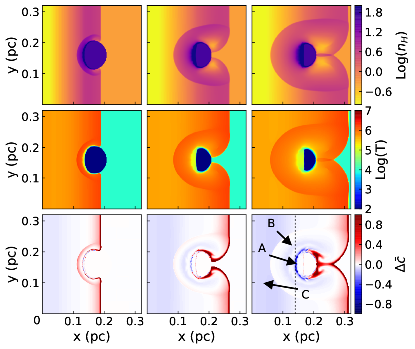
Figure 1: Three stages of the single cloud model. Time increase from left to right panels. In each column, top, middle, and bottom panels show the density, temperature, average charge difference respectively. In the bottom right panel, “A”, “B”, and “C” annotate three different recombining regions. The dotted vertical line depicts the separation of positive and negative $x$-axis component of velocity along the horizontal line through the cloud center.

In Fig. 1, we show the evolution of the shock going through a cloud. As shown in the density and temperature figures, the shock is distorted after impacting with the cloud. The distortion becomes more obvious after the engulfment, leaving a clearly cooling region due to the expansion. It has lower density and temperature than the adjacent regions in the post shock. The transmitted shock is also propagating inside the cloud with a much smaller shock velocity (in green color in the temperature figures). Some ripple features that are caused by the Rayleigh-Taylor instability occur in the compressed cloud region. Additionally, a reflected shock propagates in the reverse direction.

By using the average charge difference, we can see the ionizing gas in red (positive) and recombining gas in blue (negative) in the bottom panels. As expected, the shock front is always ionizing and the expanding regions behind the shock are clearly recombining (annotated as “C” in the last figure). The reflected shock from the cloud reheats the post-shock gas. A faint ring-like recombining feature appears between the reflected shock and the cloud (annotated as “B”). Similar to the forward shock front, it is an expanding region following the reflected shock front. In the cloud, the gas is compressed as the shock propagates. Both ionization and recombination can be seen at this region (annotated as “A”). The recombination here is probably caused by the thermal conduction in the conductive front or a mixture of the hot and cold gas, especially considering the instability features shown in this region. As indicated in this single cloud simulation, both thermal conduction and adiabatic expansion can contribute to the recombining gas around the cloud. The mechanism for the recombination is probably dominated by thermal conduction inside the cloud or on the cloud rim. The evaporated gas resulting from conduction consumes the thermal energy of the adjacent hot gas may also lead to rapid cooling (as indicated in Zhou et al., 2011) and hence recombination. In the inter-cloud regions, the recombination could probably caused by the adiabatic expansion.

3.2 SNR in homogeneous medium

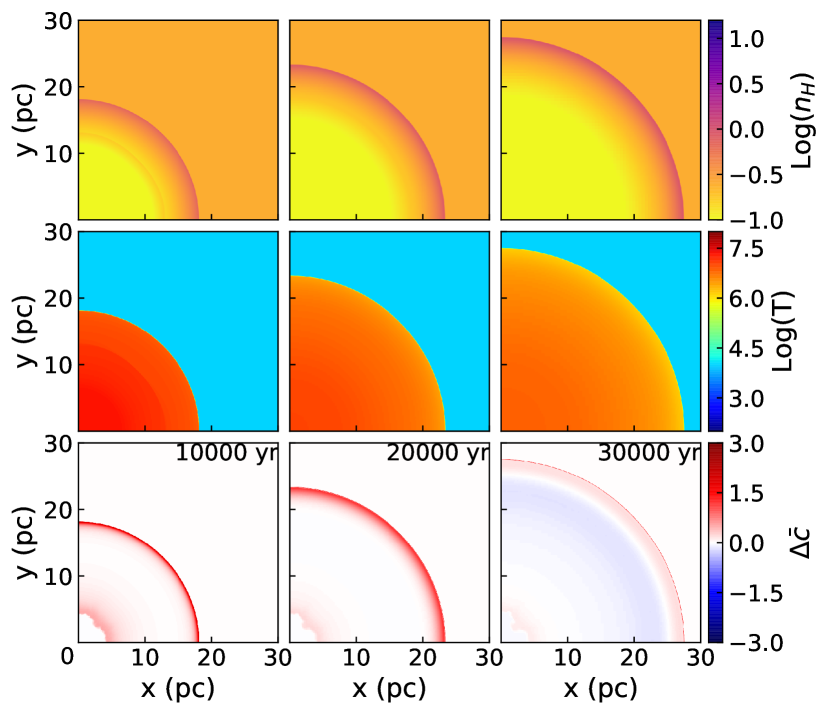
Figure 2: Three stages of the SNR model without clouds. In each column, the top, middle, and bottom panels show the density, temperature, average charge difference respectively with the same color scale. The innermost ionizing (red) features in the bottom panels are caused by the low density, which makes it harder to reach equilibrium, but does not affect the results at larger radius.

This model has a homogeneous environment, resulting a similar result with the self-similarity theoretical solution for a blast wave. Fig. 2 shows the model “B1” of a SNR in a homogeneous environment with thermal conduction. Thermal conduction smooths the temperature distribution in the interior of the SNR. The density distribution is also affected by the thermal conduction, but this does not change the shell-like shape. The spectral emission measure is proportional to the density-squared times the length along line of sight (LOS), therefore the X-ray morphology will be also shell-like, unlike the center-filled morphology shown in MMSNR. In the bottom row, the average charge difference of oxygen is shown as the indication of ionization state for this model. Before about 20000 yr, the plasma is strongly ionizing at the shock front without any obvious recombining features. The interior becomes recombining at 30000 yr, caused by the adiabatic expansion as the shock front continue moving outwards. The inner red rings at about 5 pc are the ionized gas that is slow to reach equilibrium due to the extremely low density, considering the ionization timescale $\tau=n_{e}t$. They are artifacts of the simulation which do not impact results at larger radius.

3.3 SNR in a cloudy environment

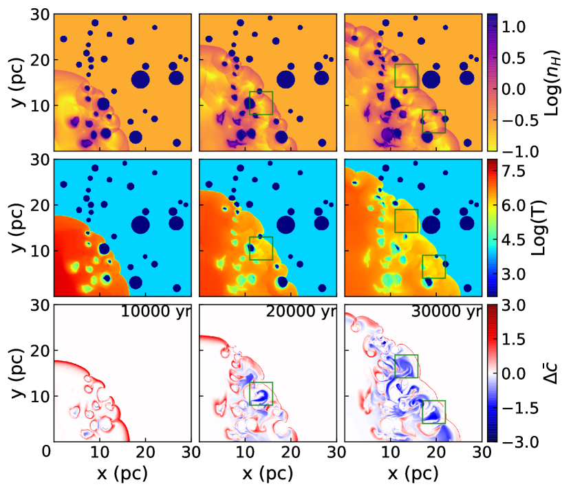
Figure 3: Three stages of the SNR in a cloudy environment model “C1” (with thermal conduction). Time increases from left to right. In each column, the top, middle, and bottom panels show the density, temperature, average charge difference respectively with the same color scale. The green boxes highlight selected recombining features that do not appear in the temperature and density maps.

Two SNR models in a cloudy environment, “C1” and “C2”, are shown in Fig. 3 and Fig. 4. In model “C1”, with thermal conduction, the clouds are evaporated after being engulfed by the SNR shock. The density in the interior then gets higher than the SNR in a homogeneous environment. In the average charge difference figures, the shock front is again always ionizing as expected; but recombining features show both in dense cloud regions and some low pressure (with low density and low temperature) regions. Some interesting features are seen in the recombining gas that do not appear in density or temperature figures (emphasized as green boxes in the figures). Comparing to the model “B1” (shown in Fig. 2), the recombination in both “C” models is more obvious, and appears earlier in the SNR interior.

As shown in Fig. 4, the clouds in model “C2” are not evaporated smoothly as in model “C1”. They are compressed and stripped with the forward shock and the reflected shock passing by. The mixing of the hot and cold gas also increases the density profile, which is moving with the shock velocities, with an almost-empty center left behind. In the average charge difference panel, recombining gas also appears in the post-shock area. However, it is in a smaller region than model “C1” with thermal conduction.

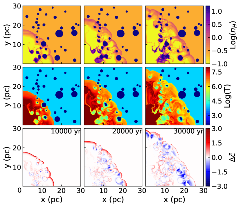
Figure 4: Three stages of the SNR model in a cloudy environment without thermal conduction (model “C2”). The layout is the same as Fig. 3.

3.4 Influence of thermal conduction on NEI

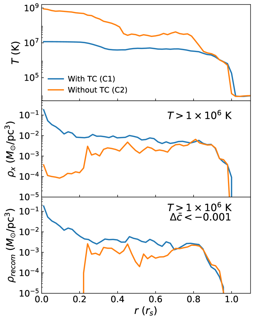
Figure 5: Average temperature (top), X-ray emitting gas density (middle), and recombining X-ray emitting gas density (bottom) along the radial direction at 2$\times 10^{4}$ yr. The blue lines are from the model “C1” (with thermal conduction; with TC), the orange lines are from the model “C2” (without thermal conduction; without TC).

From the comparison between models “C1” and “C2”, we conclude that the thermal conduction has significant influence on the NEI in SNR exploded into a cloudy environment. The top panel in Fig. 5 shows the average values of the temperature as a function of radius (in units of the shock front radius). In model “C1”, the temperature is smoothed along the radial direction, implying that the energy transfers between different layers more efficiently due to thermal conduction. Then the recombination appears when the inner hot plasma cools down rapidly. The X-ray emitting gas ($T>1\times 10^{6}\,{\rm K}$) is of primary interest. By accumulating the mass of X-ray emitting gas in different shells with a thickness of 0.5 pc, the density can be calculated as a function of radius (the middle panel in Fig. 5). Both models have a similar density profile in the shock front ($r>0.8r_{s}$). However, the thermal conduction raises the density profile in the inner layers. To investigate the recombining gas, we use $\Delta\bar{c}<-0.001$ to exclude the gas that is ionizing or in equilibrium (See appendix § B.3). A radial density profile of the recombining X-ray emitting gas is also generated with the same shell thickness (bottom panel in Fig. 5). The thermal conduction contributes to more over-ionized hot gas in the inner regions as well.

The effect of thermal conduction can be separated to be the thermal conduction that is effective in large physical scales across the remnant (Cox et al., 1999), and the thermal conduction that contributes to the evaporation of the dense clouds with smaller sizes (White & Long, 1991; Cowie et al., 1981). From our simulations, the large scale thermal conduction smooths the temperature and density distribution; and the cloud evaporation is key to the generation of a thermal X-ray emitting core and contributes to the fast cooling of the hot gas that shows over-ionized features. Because of the magnetic field in or around the SNR, thermal conduction is probably overestimated by the classical Spitzer and saturated conductivity approximation. The conductivity could be almost zero when the magnetic field is perpendicular to A high magnetic field amplification (and turbulence) is expected only when the shock velocity is high in very young SNRs that efficiently accelerate CRs (Vink & Laming, 2003; Bell, 2004; Vink, 2012; Ji et al., 2016). Therefore, this effect does not play a major role after a few thousands years of evolution. In addition to shock generated turbulence, shear flow around clouds can lead to turbulence and complex field structures that can suppress thermal conduction and mass mixing (Orlando et al., 2008). The actual effective thermal conductivity in a turbulent and magnetized environment such as SNRs evolving in a cloudy medium is uncertain. The reduction factor for conductivity relative to the unmagnetized value depends on such processes as turbulent transport and plasma instabilities (e.g.  Chandran & Maron, 2004; Komarov et al., 2016) and is an area of active study. Studies of SNR evolution in a cloudy medium that include the magnetic field, anisotropic thermal conduction and NEI would be worth pursuing in the future.

3.5 Source of recombination

3.5.1 Thermal conduction and adiabatic expansion

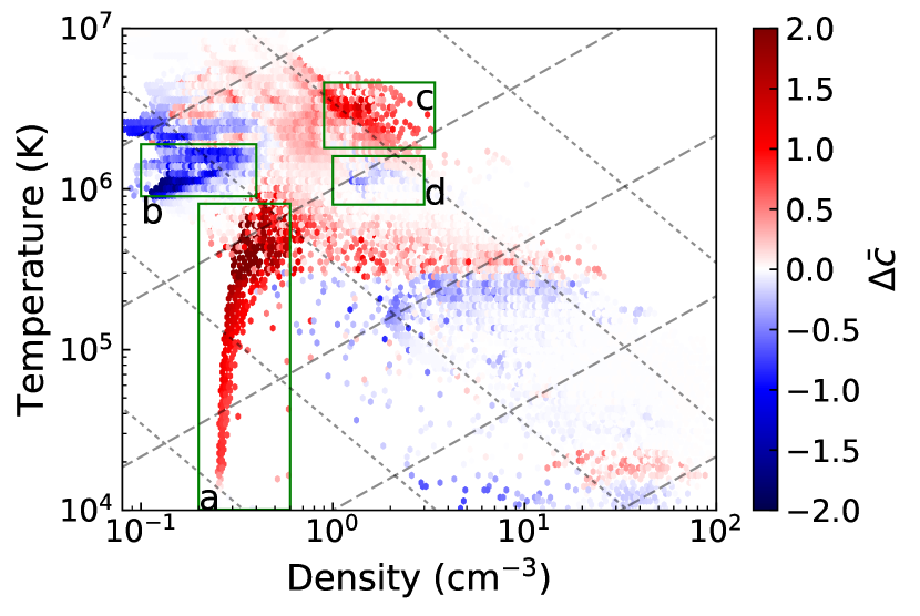
Figure 6: Phase plot of the average charge difference (for O; at 20000 yr). The dotted lines are the isobaric lines, and the dashed lines are adiabatic process lines in the phase map. Every pixel shows the average value weighted by $n_{H}^{2}$. Regions labeled “a”, “b”, “c”, and “d” are shown in Fig. 7.

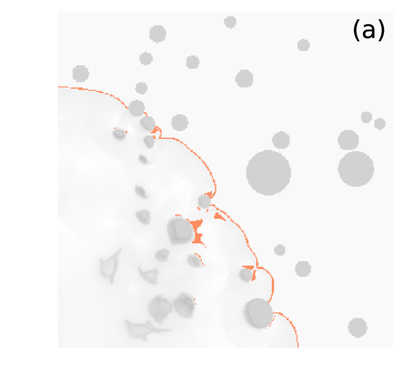
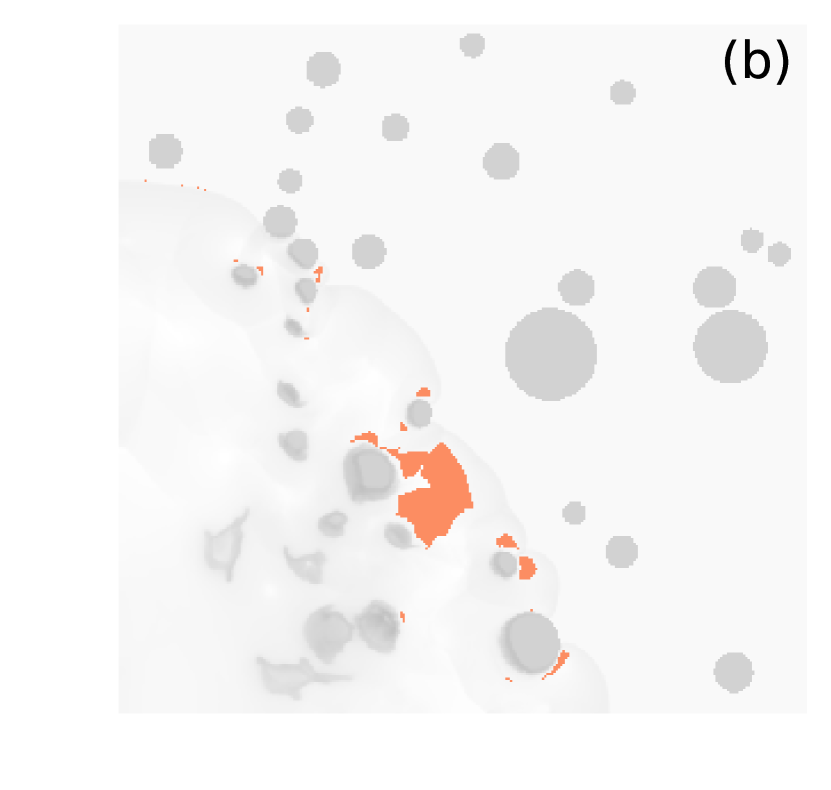
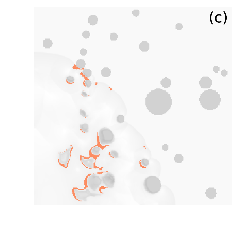
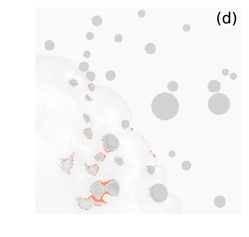
Figure 7: Positions of regions in the temperature-density phase map (Fig. 6). Grey scale is the density distribution.

i. Evolution on the phase plots.

As suggested in the single cloud simulation, there are two main causes for recombination. One is the adiabatic expansion in the inter-cloud area; the other is the energy transfer between interactions of hot and cold gas. As suggested above (§ 3.4), thermal conduction does influence the NEI process. To show the different reasons for the NEI states, we scatter-plot all the pixels in model “C1” (refined to 512$\times$512) in a temperature-density phase plot (Fig. 6). The average charge difference ($\Delta\bar{c}$) shown at each point is a density-squared-weighted average of the pixels in model “C1” with that same temperature and density.

Different physical processes can be shown in the phase plot. Thermal conduction happens whenever hot and cold materials come into contact. Assuming that the gas is in rough kinetic balance, which would not cause abrupt expansion, the change of temperature and density should keep the pressure unchanged ($T\propto\rho^{-1}$) and follow an isobaric path in a phase diagram (dotted lines in Fig. 6). When the pressure is much higher than the ambient gas, it performs a negative work, which decreases the internal energy and the temperature very quickly. Assuming that there is no internal energy exchange, the adiabatic process will follow $T\propto\rho^{\gamma-1}$ (dashed lines in Fig. 6), where $\gamma=\frac{5}{3}$ is the ratio of specific heats at constant pressure and at constant volume. In Fig. 6, one immediately apparent feature is the ionizing shock front at an almost constant density (region a). In the X-ray emitting gas, defined here as $T>10^{6}\,{\rm K}$, the ionizing and recombining plasmas seem to be separated roughly by a certain value of pressure. The ionizing gas at a higher pressure has features that appear to follow isobaric lines (region c). Below region c, there is a recombining region at a lower temperature (region d). This is consistent with the influence of thermal conduction, which can not only heat the cold gas but cool the hot gas. The recombining gas at a lower pressure (bottom left of the figure) has some features that suggest it could be adiabatically expanding (region b). To check the physical positions of the gas in different ionization state, the regions a, b, c, and d in Fig. 6 are shown in orange in Fig. 7, overlapping a density distribution to show the cloud distribution. The map of region a is consistent with the shock front and some ionizing regions behind clouds (See Fig. 1 for a similar ionization distribution). Recombining region b is in the post-shock region behind some clouds, which should be in expansion. Ionizing region c and recombining region d seem to be next to the cloud regions. These are likely compressing regions, where thermal conduction dominates the cooling process.

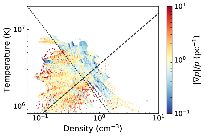
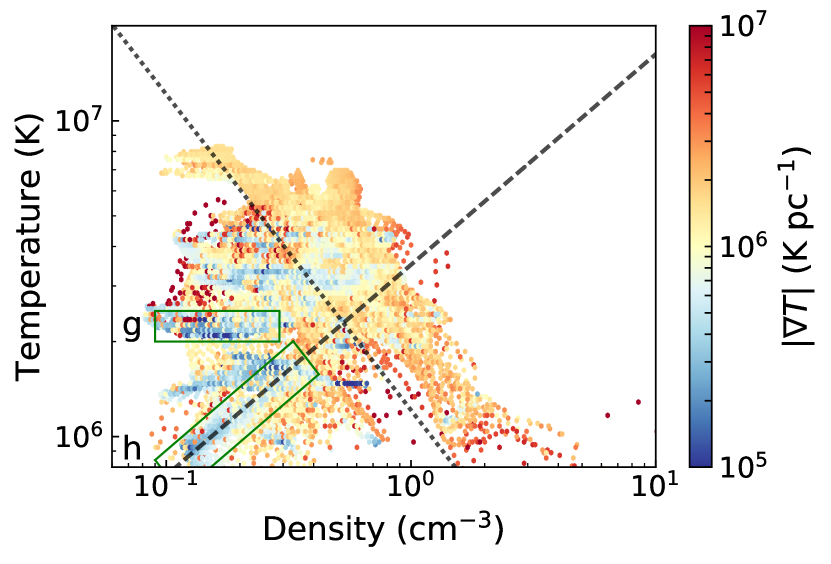
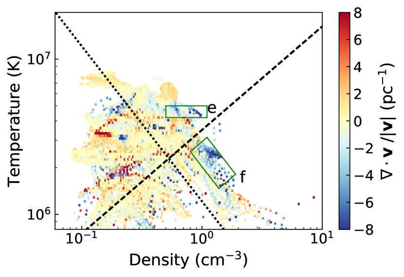
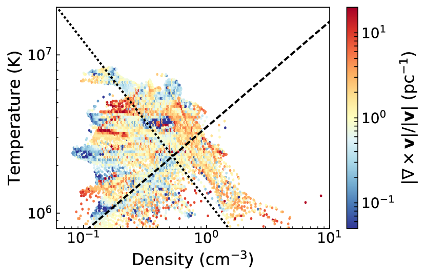
Figure 8: Phase plot (for O; at 20000 yr) for recombining plasmas with the magnitudes of relative gradient pressure vectors (top left), temperature gradient vectors (top right), relative velocity divergence, and relative vorticity in color. The dotted line is the isobaric line for pressure 3.5$\times 10^{-10}\,\rm g\,cm^{-1}\,s^{-2}$, and the dashed line is an adiabatic process line. Four regions in the phase plot are also shown in the spatial distribution in Fig. 9.

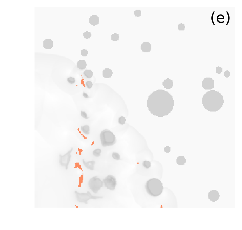
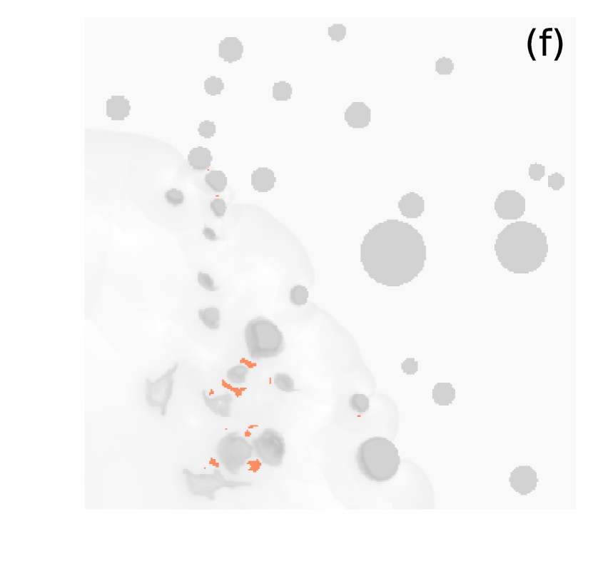
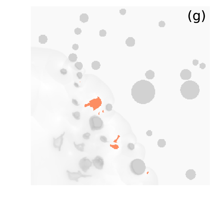
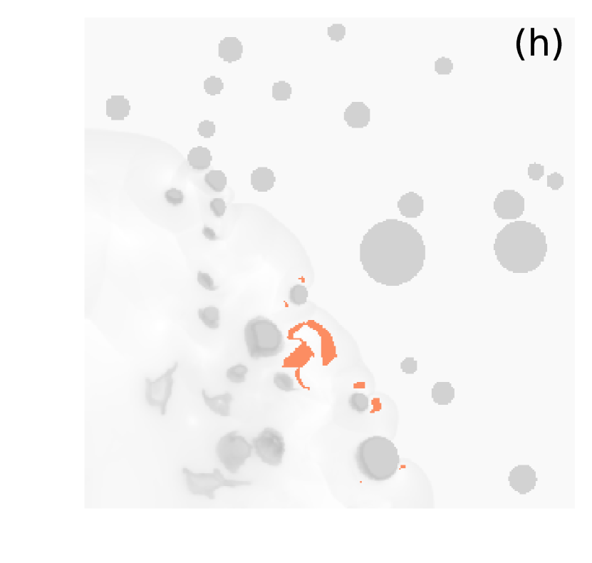
Figure 9: Selected regions in the temperature-density phase map of recombining plasmsas. (Fig. 8). Grey scale is the density distribution. The recombination process in regions (e) and (f) seems to be driven by thermal conduction, while in regions (g) and (h) it is dominated by adiabatic expansion.

Considering the ultimate goal of connecting the X-ray observations to the underlying physical properties (see also appendix B), Figures 6 and 7 imply the NEI amount (e.g. $|\Delta\bar{c}|$) is less important than the sign of $\Delta\bar{c}$. In the phase diagram (Fig. 8) we show a range of quantities measured in the recombining plasma only (defined as $\Delta\bar{c}<-0.001$). The partial differential (of gradient, divergence, and curl) calculations adopt a central finite difference method. The value of each point in this figure is the average value of the simulation pixels that are recombining with the same temperature and density. There are regions in this figure that can be analyzed to determine the dominant physical reason for the recombination. Thermal conduction, for example, needs a high temperature difference between the conducting materials ($\nabla T$), while adiabatic expansion has a positive velocity divergence ($\nabla\cdot\vec{v}>0$). In the top left panel of Fig. 8, the pressure gradient is relatively low at a higher pressure. When the pressure gradient is high in a low pressure environment, the plasmas are in an unstable state, and dynamical processes should dominate the temperature changes. In the top right panel, there are some features in the bottom left with a low temperature gradient, corresponding to the higher relative pressure gradient areas in the top left panel (such as region g and h). In these regions expansion cooling could dominate, especially as some of them appear to follow an adiabatic path (region h). In Fig. 9, regions g and h are all in inter-cloud regions that are also in between the shock front and cloud regions, also suggesting an adiabatic expansion cooling. In the bottom left panel of Fig 8, the velocity divergence shows whether the plasmas are expanding ($\nabla\cdot\vec{v}>0$, in reddish color) or compressing ($\nabla\cdot\vec{v}<0$, in blueish color). Regions with a negative velocity divergence, such as region e and f, are not in expansion so the adiabatic expansion could not contribute to the cooling in these regions. In the top right panel, thermal conduction could dominate with a high temperature gradient in the same areas. In the bottom right panel, the magnitude of vorticity depicts how the materials are mixing together. The fluid instability that happens on the contacting surface of gas increases the vorticity. Expanding regions tend to have a low vorticity on the contrary. Regions e and f have a high vorticity, also suggesting the hot and cold plasmas are contacting with each other. In Fig. 9, the map of region e seems to be in some complex cloud areas. Complex reflected shocks collide with each other. Region f seems to be on the rims of clouds, where the thermal conduction should dominate the cooling. It should be noted that both mechanisms can contribute the recombination all over the phase map in previous time steps rather than the current time step. The recombination may not be consistent with cooling, because there are some recombining gas parcels reheated without enough time to change the ionization state.

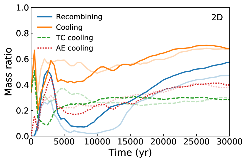
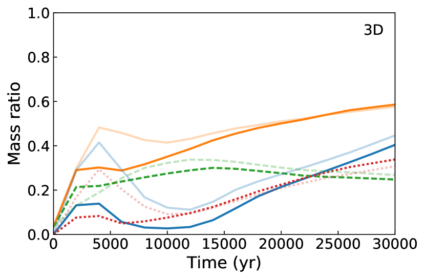
Figure 10: The mass ratios of recombining plasmas, cooling plasmas, thermal conduction dominant cooling plasmas, and adiabatic expansion cooling plasmas in 2D simulations (left) and 3D simulations (right) as a fraction of the total X-ray emitting gas mass($T>1\times 10^{6}\,{\rm K}$). A different random cloud distribution (with the same WLC parameter) is shown for both 2D and 3D simulations in translucent lines.

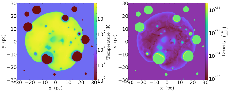
Figure 11: The temperature (left) and density (right) distribution of a slice plane at $z=0$ of the 3D simulation (at $2\times 10^{4}\,{\rm yr}$).

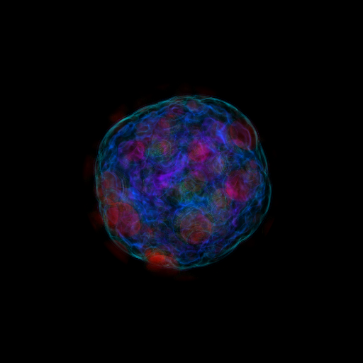
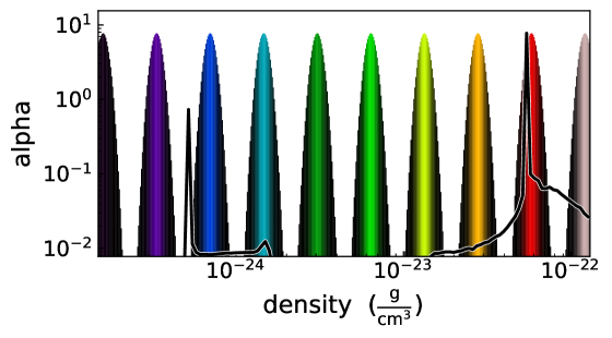
Figure 12: The density distribution of 3D simulation (at $2\times 10^{4}\,{\rm yr}$) with a volume rendering method. The transfer function of the volume rendering is shown in the bottom panel, where the histogram of density is shown in black. From left to right, the first peak of the black line is at the initial density of the inter-cloud ISM, corresponding to a white region (the volumes with this density are left transparent). At the right wing of this peak, it is the density of shocked ISM, which is shown in blue and cyan. The second peak is the initial density of the dense clouds, corresponding to the red color in the top panel. All the clouds farther than $25\,{\rm pc}$ are excluded.

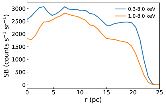
Figure 13: The radial surface brightness of the projected 3D simulation at 2$\times 10^{4}\,{\rm yr}$ with a range of energy (0.3–8.0$\,{\rm keV}$ and 1.0–8.0$\,{\rm keV}$). The element abundances are assumed to be solar abundance and the emission model is assumed to be CIE (“apec” model in Xspec). The photons are collected with the Athena instrument response. The harder band (1.0–8.0$\,{\rm keV}$) uses a higher exposure time (See the text).

ii. Mass ratio of cooling components.

In view of the hydrodynamic evolution, the reason for recombination can be estimated by the temporal evolution of the cooling material. With the hydrodynamic equations in Lagrangian scheme, the internal energy change can be obtained with the equation,

$$\frac{\mathrm{d}U}{\mathrm{d}t}=-c^{2}\nabla\cdot\vec{v}+\frac{1}{\rho}\nabla\cdot(\kappa\nabla T),$$ (2)

where $U$ is the internal energy relating to $T$, $\rho$ is the density, $c$ is the sound speed, $\vec{v}$ is the velocity vector, and $\kappa$ is the thermal conductivity. If only the cooling is considered, the first term is the adiabatic expansion cooling, and the second term is the thermal conduction cooling. We can hence calculate both of the terms for a given parcel to determine whether it is cooling or heating. In cooling parcels, if the absolute value of the first term is greater than the one of the second term, the adiabatic expansion is dominant (AE cooling); if the absolute value of the first term is smaller than the one of the second term, the thermal conduction is dominant (TC cooling). In the heating parcels, the dominant term can be determined with the same method. By summing up the mass in these categories, we can know how much of the gas is cooling versus heating and ionizing versus recombining. As we are interested in the X-ray recombination phenomenon, Fig. 10 plots the mass fraction of some categories, including cooling, TC cooling, AE cooling, and recombining mass in the total hot gas ($T>1\times 10^{6}\,{\rm K}$) mass. In the 2D models, at an early stage, one or two of the clouds are engulfed, making the cooling mass and recombining mass fraction increase abruptly. The AE cooling also seems to exceed TC cooling. Later at around 10000 yr, the recombining mass proportion rises again. In the period from 5000 yr to about 15000 yr, TC cooling exceeds AE cooling. From Fig. 3 (bottom left panel), the recombining plasmas are mainly in the clouds area, implying the thermal conduction could possibly be the dominant term for the recombination during this time. The thermal conduction cooling mass remains nearly a constant, which is expected considering the evaporation of clouds does not change dramatically (as shown in Slavin et al., 2017). The adiabatic expansion proportion exceeds the thermal conduction at an even later time. Some of the mushroom features in the late time recombining images (Fig. 3) also suggest a contribution of adiabatic expansion.

3.5.2 The simulations in 3D

In the 3D simulation, the total number of clouds increases over the 2D model. The clouds are spheres instead of rings in 2D cylindrical simulations. But the hydrodynamic behaviors are similar in a slice plot of the 3D simulation (See Fig. 11 and Slavin et al. 2017). However, with the symmetry, 2D simulations will be affected by the clouds on or near the $z$-axis and $x$-axis. In Fig. 3, we can see that the clouds are distributed closer around $x$-axis than the one around $z$-axis. This effect causes a little higher temperature around $z$-axis. A full volume 3D simulation can avoid this effect. In Fig. 11, the slice plots in the 3D simulation show that the distribution of temperature and density are affected by the distribution of the clouds. With the Python module yt-project, a 3D volume rendering figure is shown in Fig. 12. The color coding is tuned to show the shock front in cyan and the dense clouds in red. The shape of SNR that is distorted by the distribution of the dense clouds is not symmetric. The cyan filaments showing the shock front are formed by the projection effect.

From the 3D simulation, we generated X-ray photons in each pixel according to the emission model and the physical properties in situ and projected them onto an X-ray observation instrument (XIFU on Athena). By assuming that the plasma is in CIE (“apec”) and all the metal abundances are solar abundances (Anders & Grevesse, 1989), Fig. 13 shows the average surface brightness as a function of radius. In the X-ray band from 0.3$\,{\rm keV}$ to 8$\,{\rm keV}$, the thermal emission is centrally brightened. Since MMSNRs are almost always heavily absorbed, the energy range from 1$\,{\rm keV}$ to 8$\,{\rm keV}$ has been shown in this figure as well. The surface brightness in the center ($r<5\,{\rm pc}$) is lower, which might be caused by the empty center ($r<2.25\,{\rm pc}$) in the initial condition. Here, the smaller energy range ($1\,{\rm keV}$–$8\,{\rm keV}$) has an exposure time of 1000$\,{\rm ksec}$; and the larger one ($0.3\,{\rm keV}$–$8\,{\rm keV}$) use a shorter exposure time (100$\,{\rm ksec}$). In the appendix §B we describe the details to generate simulated observations, and make use of the NEI information in the simulations.

We have also produced the figures like Fig. 3, Fig. 6, and Fig. 8 for 3D as well. They are similar to the figures of 2D, albeit with lower resolution. The 2D simulations are shown here because the spatial distribution is easier to illustrate in 2D than 3D. In the right panel of Fig. 10, the mass ratio of recombining and cooling components is shown for 3D simulations. The time resolution is sparser because of the considerable sizes of the files. It is hard to investigate the early stages (about 2000 yr to 4000 yr) when the AE cooling and TC cooling components change dramatically. The crossing of these two components at the late stages is postponed from about 16000 yr to 23000 yr, because of more fragmentary clouds. In both 2D and 3D simulation, the choice of distribution does not change the conclusion about the sources of recombination.

We close this section by noting several key points.

1. We tested multiple different sets of random clouds distribution with the same WLC. Although the results are not exactly the same, the overall trend is unchanged.

2. The cooling or heating components are shown as a function of their mass, not the total energy change. Thermal conduction can both heat and cool two groups of gas that are contacted simultaneously, leaving the total energy transfer as zero.

3. With a lower limit (10${}^{6}\,{\rm K}$) to the temperature, both thermal conduction and adiabatic expansion can cool an X-ray emitting gas to be X-ray-quiet. However, a cool gas can also be heated to an X-ray emitting gas. So if the heating and ionizing components are analyzed, the lower limit in temperature will underestimate the gas being heated. Since we focus on the recombining component in this paper, it does not impact our conclusions.

4. The times given here are for a specific ambient density. Different SNR observations should be compared to the simulation with corresponding initial conditions to make sure the evolution age is valid.

4 Discussion

4.1 Applications of the simulations to observations

With the spatial resolution in X-ray observations, a temperature-density diagram can show the relative position of each region in the phase map as the one in Fig. 8. Fig. 14 is an example for a W49B observation (Zhou & Vink, 2018) with an adiabatic expansion line and an isobaric line shown as dashed and dotted lines. The error bars are from the 90% confidence ranges of the hot component fitting, where the errors from the cool component fitting are not included. Only recombining (timescale $\tau<1\times 10^{13}\,{\rm s}\,{\rm cm}^{-3}$) hot components are shown in the phase diagram (right). The colormap shows the relative difference between the fitted temperature of hot components and the cooler components. It seems the low pressure regions tend to have a smaller relative temperature difference. If the two components are assumed to be thermally conducting, the smaller the temperature difference the smaller the thermal conduction flux. Of course, this is not the same as a true thermal gradient; the two components may not be in actual contact but merely in the same line of sight. The points along the isobaric line with larger temperature differences show a probable thermal conduction contribution to the overionization. The points in the south west of the SNR with smaller temperature differences seem to be along an adiabatic expansion line in the phase diagram, which could be a strong hint for an adiabatic expansion dominance. With more X-ray instruments coming on board, the phase diagram can be a useful tool to diagnose the NEI process in SNR plasmas.

The distribution of the overionized plasma also depends on the SNRs’ immediate environment. In the case of W49B, it was also suggested that both thermal conduction and adiabatic expansion resulted in the overionized plasma, but a density enhancement of the ambient medium is assumed near the SNR center. In the numerical simulation of Zhou et al. (2011), it was also suggested that both thermal conduction (mixing of hot and cold plasma) and adiabatic expansion resulted in the overionized plasma in W49B, but a density enhancement of the ambient medium is assumed in the SNR interior. This scenario is recently supported by (Zhou & Vink, 2018). On the other hand, Miceli et al. (2010) proposed a scenario that W49B requires dense clouds close to the explosion center. When the blast wave and the ejecta break out into the surrounding low-density region, the plasma cools down rapidly and becomes overionized. It also supports the adiabatic expansion origin of the overionization. This scenario has been supported by Lopez et al. (2013); Yamaguchi et al. (2018) and also been proposed for SNR IC 443 (Greco et al., 2018).

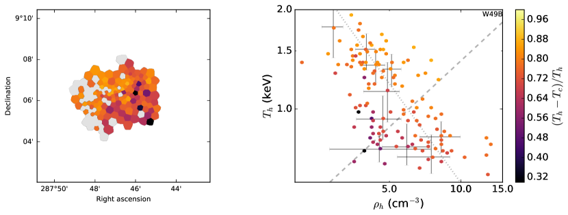
Figure 14: The relative temperature difference between the hot component and the cold component in a W49B X-ray observation (Zhou & Vink, 2018) is shown in the left panel with the equilibrium points shown in gray. Recombining hot components in W49B (with the subscript of $h$) are scattered into the temperature-density phase diagram (right panel). The dashed line depicts an adiabatic evolution path and the dotted line depicts an isobaric line. Similar to Fig. 8, bottom left points in the phase map tend to have low temperature difference, supporting an adiabatic expansion origin. Ten random points are chosen to show the error bar (90% confidence).

4.1.1 Turbulent mixture

In the ISM the turbulent mixing of plasma is common (Slavin et al., 1993), which could be another source of over-ionization. When gas with different properties is advected into one of the highest resolution cells in a hydrodynamic simulation, the physical properties are effectively averaged. The density, $\rho$, is averaged with volume weighting. The temperature is calculated from the internal energy every time step and is averaged with mass weighting, $T=\frac{T_{1}m_{1}+T_{2}m_{2}}{m_{1}+m_{2}}$. The ion fraction for an element $f^{(i)}$ ($i=0,1,2...Z$, $Z$ is the atomic number) is also averaged with mass, $f^{(i)}=\frac{f^{(i)}_{1}m_{1}+f^{(i)}_{2}m_{2}}{m_{1}+m_{2}}$. Therefore the average charge can be expressed as $\bar{c}=\sum\limits_{i=0}^{Z}f^{(i)}c_{i}=\frac{\bar{c}_{1}m_{1}+\bar{c}_{2}m_{2}}{m_{1}+m_{2}}$. From Fig. 15, it can be seen that the equilibrium average charge is not linear with temperature. Even assuming the gas is in CIE before the mixing, it can become effectively out of equilibrium as a result of mixing. However, since the ionization is roughly linear over small ranges of temperature, mixing between materials with similar temperature will not cause substantial deviation from CIE. Mixing is thus similar in its effects to thermal conduction. Thermal conduction does not mix materials directly, but the internal energy is redistributed from the hotter to cooler gas. With enough elapsed time, this process also occurs when physically mixing plasmas. This becomes complex in a numerical simulation, however, because numerical viscosity and the effects of finite resolution, both of which are connected to the simulation resolution, can create unphysical mixtures. By comparing different resolutions (See § 2) of 2D simulations, we confirmed that the results shown above change very little. In 3D simulations, with different resolutions, the slices of runtime variables look the same, and the mass of hot gas used in Fig. 10 changes less than about 1.5%, which we deemed acceptable. More computation power is needed to find how much a better resolution could improve these conclusions in 3D simulations.

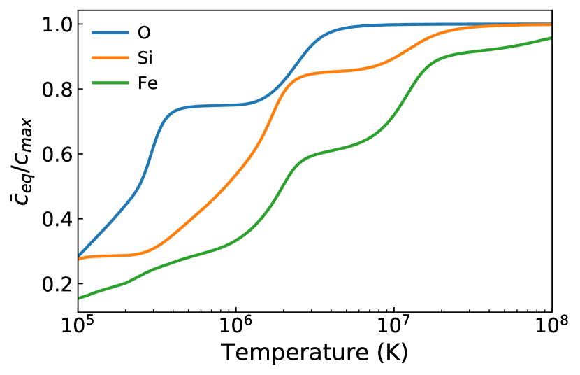
Figure 15: CIE average charge of different elements (O, Si, and Fe) as a function of temperature. $C_{max}$ is the maximum charge for each elements (8, 14, and 26 respectively).

4.2 Selection of elements and the ionization energy

We use oxygen for most of the analysis in this work. Other elements can be used too. As suggested by observations, some heavier elements, like Si, Mg, Fe, are easier to observe because of the high absorption commonly seen in MMSNR. However, the assumption of an equilibrium between the ion temperature and electron temperature should be carefully treated for those elements who are sensitive to electron temperature around $10^{7}\,{\rm K}$ (Fig. 15). The electron temperature can be about $10^{7}\,{\rm K}$, while the ion temperature is a factor of ten higher (e.g.  Patnaude et al., 2009).

Although the ionization of some elements are taken into account, the energy change from ionization and recombination is not calculated in current simulations. Considering the cosmic abundance of elements, heavy elements will not contribute much to the total energy. Both hydrogen and helium, however, will effectively ‘store’ energy in their ionized states. The energy will be released mainly into photons when they recombining back to lower states. H and He have an ionization energy of 13.6 eV and 79 eV (fully ionized) respectively. By assuming the mass ratio of He 0.79, and H 0.21, the ionization energy in a unit mass is $E_{ion}=\frac{0.21}{m_{H}}\times 13.6\,{\rm eV}+\frac{0.79}{m_{He}}\times 79\,{\rm eV}$. If 100 $M_{\odot}$ is swept by the SNR shock, $3\times 10^{48}\,{\rm erg}$ (3% of the explosion energy) is needed for a full ionization. In fact, most ISM gas in our simulations is in a full ionization or partially ionization state of H and He because of the fluctuation around temperature $1\times 10^{4}K$. Similarly, we can know the dissociation energy for hydrogen molecules for the same swept mass is about $4\times 10^{47}\,{\rm erg}$ (0.4% of the explosion energy). It can then be assumed that the hydrogen and helium ionization does not affect the hydrodynamic evolution.

4.3 Other possible effects

Some observations have found metal-enriched materials inside the SNRs (Zhang et al., 2015). The ejecta in SNR could affect the final results too, because it has a larger metallicity than the ISM. After the shock front reaches about 10 pc from the explosion center the swept mass will be larger than the ejecta for ordinary SNRs (ejecta mass is less than 8 $M_{\odot}$). We ignore the abundance from the ejecta as we focus on the late stages of the SNR evolution. A further investigation of simulations should be done with ejecta in the future for a more realistic model.

It is generally accepted that some of the high-energy cosmic ray (CR) particles are accelerated in SNR, which could also be a source of the recombination. The electrons in the ions are kicked out by the high-energy CR, appearing to be over-ionized in the current temperature environment. The acceleration process depends on the magnetic fields around the shock front. As no magnetic field is included in these simulations, we did not include this process.

Patnaude & Fesen (2005) have found that the interaction between a shock and a cloud with a smooth varying density changes the hydrodynamic instability from a sharp-edged cloud. In addition, the ISM environment should be turbulent as simulated in Zhang & Chevalier (2018), rather than a distribution of round clouds. To make a further comparison with observations it will be needed to consider a turbulent environment with different cloud density gradients, which we plan for a future project.

5 Conclusions

Including NEI calculations, several 2D and 3D SNR simulations are performed. As expected, the shock front is always ionizing and the SNR in a homogeneous environment has a good consistency with the Sedov-Taylor self-similarity solution. Both ionization and recombination can be seen in the interior of the SNR with a cloudy environment. Both a direct analysis of the simulation results and a mimicked X-ray observation toward the SNR simulation are used. The thermal conduction is estimated for the contribution to the NEI. Especially for the cooling X-ray emitting plasmas, thermal conduction could contribute in a similar amount as the adiabatic expansion.

Appendix A Compare model “B2” with the theory

From the self-similarity solution, the shock radius is $r_{s}\propto t^{\frac{2}{5}}$, and the shock velocity is $v_{s}\propto t^{-\frac{3}{5}}$. To compare to the ionization state we set a strong shock model with shock front satisfying

$$\frac{\rho_{2}}{\rho_{1}}=\frac{v_{1}}{v_{2}}=4$$ (A1)

where $\rho_{1}$, $v_{1}$ and $\rho_{2}$, $v_{2}$ are the density and velocity in the upstream and downstream respectively. At a later SNR age (e.g. after 10000 yr), shock front temperature, $T_{s}\propto v_{s}^{2}$, is higher than 10${}^{7}\,{\rm K}$ where the ionizing rates of O⁶⁺ and O⁷⁺ change relatively slowly. By assuming the shock front temperature does not change during a time interval, we can calculate the ion fractions for several points in the post shock area (See dotted lines in Fig. 16). For each point, the initial ion population is adopted from the upstream values (right side in the figure), the temperature and the electron density are adopted from the theoretical value in situ. The time interval is calculated by $\Delta t=\Delta r/v_{2}$, where $v_{2}$ is the downstream velocity in the shock front reference frame. The maximum value of $v_{2}$ is $\frac{1}{4}v_{\rm s}$, and $v_{s}$ is the shock front velocity, changing with the shock front radius $r_{s}$ or time $t$ according to the self-similarity solution. The materials in the upstream are assumed to be equilibrium. The ion fractions in equilibrium and the ionization rates when it enter the shocked area are calculated with values from AtomDB (Foster et al., 2012). However, the time interval for a parcel of gas moving from the shock front $r/r_{s}=1$ to a downstream point at $r/r_{s}=0.8$ takes about 6000 yr. The ionization history is not the same for the points in the downstream. To make a closer estimate from the theoretical model, for every 0.01 of $r/r_{s}$, the ionization histories are corrected to a strong shock with physical parameters adopted from the self-similar equations,

$$r_{s}\propto t^{2/5}$$ (A2)

$$v_{s}\propto t^{-3/5}$$ (A3)

$$T_{s}\propto t^{-6/5}$$ (A4)

The radial profiles for temperature, velocity are recalibrated for the self-similar solution, where the density profile will not change because of the fixed compressing ratio. Fig. 16 shows that the time corrected model gets closer to the simulation with some zig-zag features caused by the sparse correction, although the real history is more complicated. Here, the model “B2” (without thermal conduction) is plotted as solid lines to compare with the theoretical model.

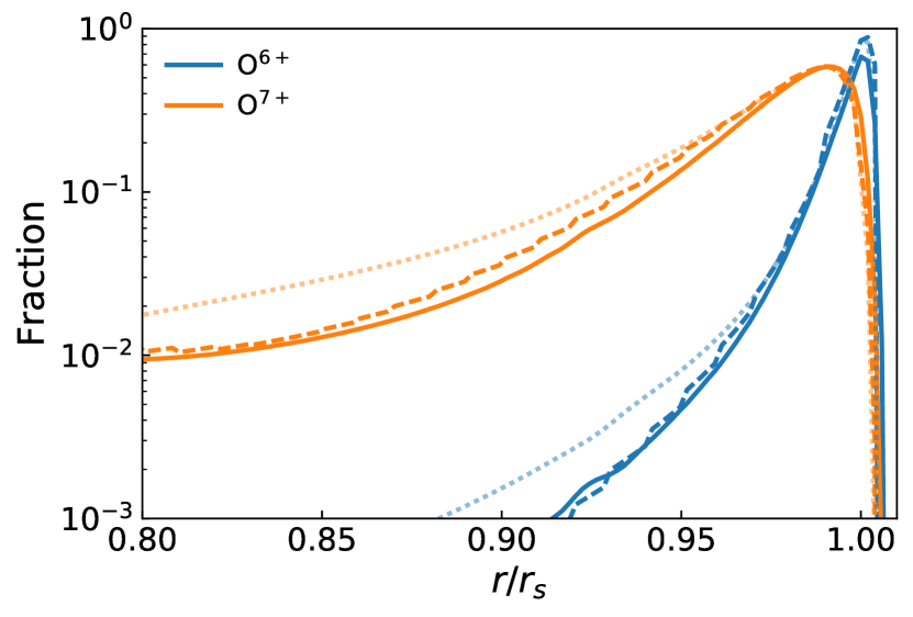
Figure 16: Ion fractions (O⁶⁺ and O⁷⁺) at the shock front of an SNR in homogeneous environment (10000 yr). The solid lines are from the simulation without thermal conduction. The dotted lines are from the estimation of a theoretical Sedov-Taylor self-similarity solution of the blast wave. The dashed lines are the same theoretical model with the ionization history modified every 0.01 in the horizontal axis. (See the text).

Appendix B Simulated X-ray observations

B.1 Spectrum generation method and the single point test

Although we can determine the ionization state with the average charge as discussed in our previous work (Zhang et al., 2018), a simulated spectrum remains the best way to compare directly with the SNR observations. From the 3D simulation, we can generate a simulated spectrum with the physical properties of the final results, using Python scripts SOXS and pyXSIM. It is assumed that the hydrogen in the simulation is fully ionized, which is true when the temperature is much larger than $1\times 10^{4}\,{\rm K}$. Considering the X-ray emission temperature is above about $1\times 10^{5}\,{\rm K}$, the exact hydrogen ion fraction will not significantly affect the spectrum. The SOXS and pyXSIM codes generate a list of X-ray photons based on the non-equilibrium spectrum (including Doppler velocities) at every position in the 3D simulation. By projecting the photons onto a simulated X-ray telescope, an event file is obtained that can be used to create images and spectra. We modeled data from three X-ray instruments: the Resolve Instrument on XRISM, the X-IFU on Athena, and the LXM on Lynx.

To test the spectral generation, both a single ionizing and a recombining pixel in the simulation were selected. By fitting the spectra, we have compared them to the actual physical quantities in the pixels. the fit results from both the ionizing and recombining spectra are consistent with the simulation. Here is an example pixel with an electron temperature 0.62 keV in the simulation. Ignoring Doppler shifts for simplicity, the simulated spectrum from this one pixel, observed in a 100Ms Athena X-IFU exposure, is shown in Fig. 17[Left]. We fit the spectrum using the Xspec vrnei model, which assumes a gas parcel in equilibrium at an initial temperature is then instantaneously heated (or cooled) and held at a new temperature. In the fit, the initial temperature was indeterminate and fixed to a maximum value of 10$\,{\rm keV}$. The best-fit electron temperature is $0.605\pm 0.002$, only 3% from the simulation (See Table 4). Nonetheless, this is a $7.5\sigma$ difference; we expect this systematic offset is primarily due to using a simplified model (vrnei) that does not capture all of the changes this particlar cell in the 3D simulation has undergone. With the fit parameters and pyAtomDB, we can also compare the ion fractions predicted by the vrnei with those in the cell itself; these are shown in the right panel of Fig. 17. We conclude that this fit is largely consistent with the original data.

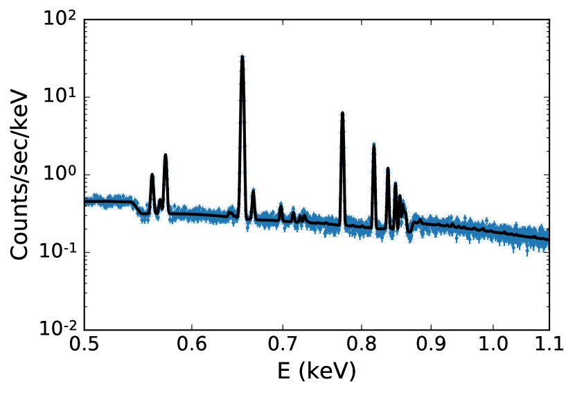
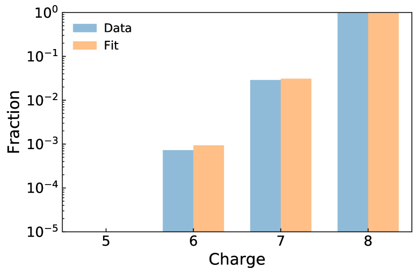
Figure 17: A test spectrum from a single point in the simulation. The spectrum and the fit model are shown in blue and black in the left panel (See Table 4). The ion fraction distribution (oxygen) that is obtained with the fit parameters is shown in the right panel with the original ion fraction from data as a reference.

Table 4: Single point spectrum fit (vrnei)

Parameter	Unit	value
kT	keV	0.605$\pm 0.002$
kT_init	keV	10
Tau	s/cm3	$(1.92\pm 0.09)\times 10^{11}$
norm		$(8.47\pm 0.02)\times 10^{-5}$
$\chi^{2}\tablenotemark{$\ddagger$}$		1.23 (3870)

B.2 Observations with Athena, XRISM, and Lynx

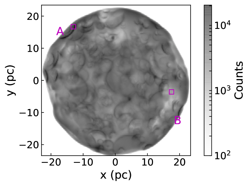
Figure 18: Simulated Athena XIFU observation from a 3D simulation with projection along $z$-axis. The gray scale depicts the distribution of generated events. The positions to extract Spectrum A and B have been labeled.

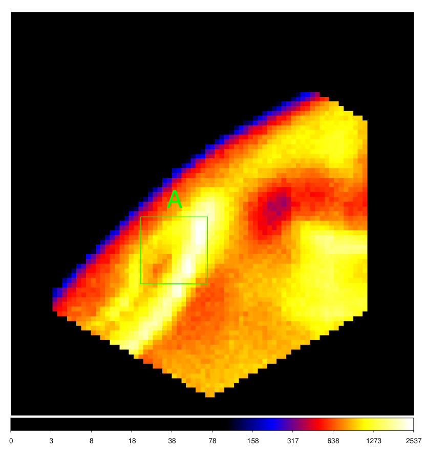
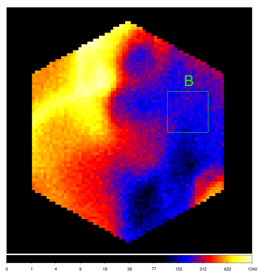
Figure 19: Two simulated observations with Athena. Spectrum A and B are extracted from the corresponding boxes in these two observations.

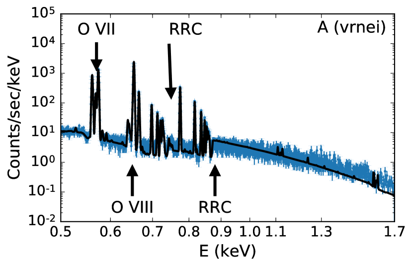
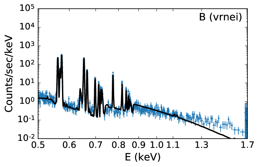
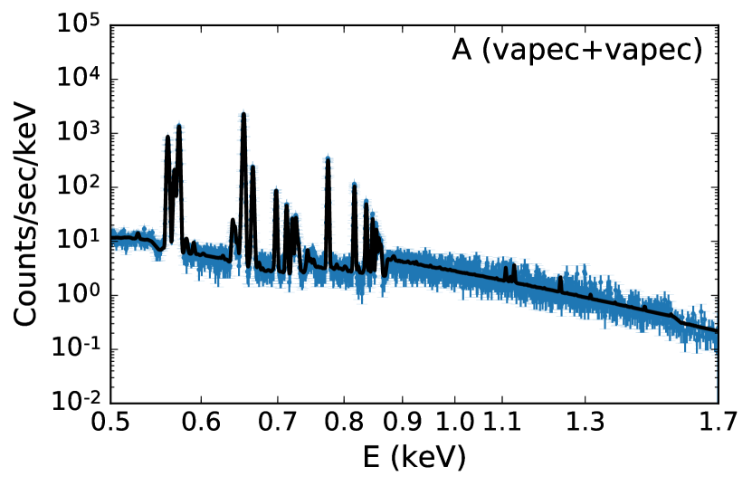
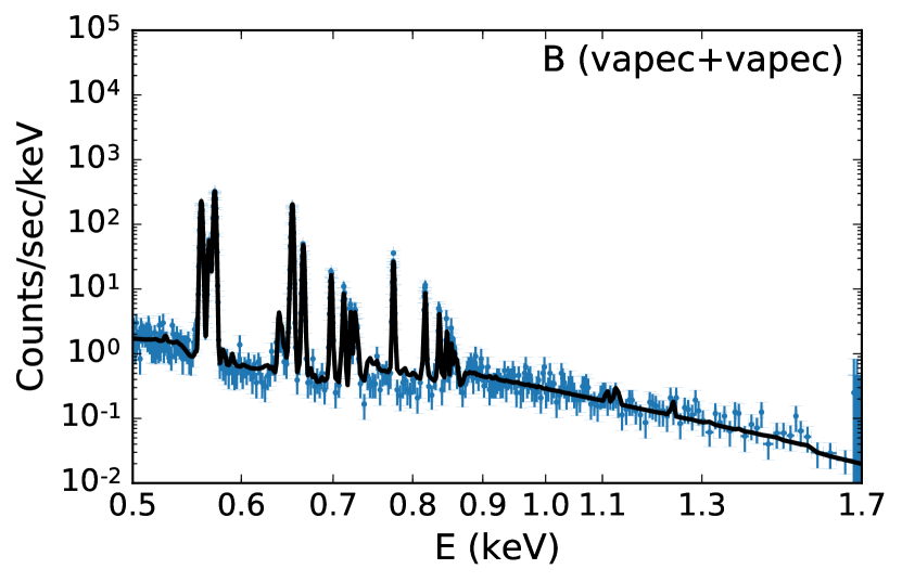
Figure 20: Two example spectra (A and B) are shown below with the spatial regions depicted in the top panel. Both the spectra A and B have an exposure time of 10 ks. They are fitted with a “vrnei” model and a two-component “vapec” model. The fit results are listed in Table 5 and Table 6.

Table 5: Fit parameters with vrnei model

Parameters	Unit	Spectrum A	Spectrum B
kT	keV	0.2183 $\pm 0.0006$	0.164 $\pm 0.001$
kT_init	keV	10	10
Tau	$\,{\rm s}/{\rm cm}^{3}$	$(8.8\pm 0.1)\times 10^{11}$	$(1.34\pm 0.03)\times 10^{12}$
norm		$(2.53\pm 0.02)\times 10^{-3}$	$(4.90\pm 0.10)\times 10^{-4}$
$\chi^{2}\tablenotemark{$\ddagger$}$		3.21 (1704)	1.75 (512)

Table 6: Fit parameters with two vapec models

Parameters	Unit	Spectrum A	Spectrum B
kT_c	keV	0.212$\pm 0.002$	0.157$\pm 0.003$
kT_h	keV	0.45$\pm 0.02$	0.46$\pm 0.03$
norm_c		$(1.66\pm 0.02)\times 10^{-3}$	$(4.03\pm 0.09)\times 10^{-4}$
norm_h		$(8.06\pm 0.47)\times 10^{-4}$	$(9.98\pm 0.7)\times 10^{-5}$
$\chi^{2}\tablenotemark{$\ddagger$}$		2.38 (1703)	1.30 (511)

The simulated SNR model (with the age of 2$\times 10^{4}\,{\rm yr}$) was assumed to be at a distance of 5 kpc, with no absorption.Using the response and field of view of the Athena X-IFU instrument (Nandra et al., 2013; Barret et al., 2018), 59 10 ksec observations are adequate to cover the entire SNR. In Fig. 18, the X-ray events distribution image in energy range from 0.35 keV to 1.7 keV shows the projected hot gas distribution inside the SNR. There are some ring or concave features in some areas, likely corresponding to the partially shocked clouds. Two example observations are shown in Fig. 19 with the X-IFU field of view. For each observation, twelve spectra are extracted in box regions (with a size of 1′$\times$1′each).

With a vrnei model in Xspec, they can be fit to determine whether it is recombining. Here we only use oxygen in solar abundance for lines with hydrogen and helium mainly contributing to the continuum; other elements are set to zero. The electron number density can be calculated from the fitted parameter “norm” in the model vrnei. A spherical ball of X-ray emitting gas with a filling factor of 1 is assumed to get the volume of the observation area. The depth of the X-ray emitting gas is $L=\sqrt[]{R^{2}-r^{2}}$, where $R$ is the average radius of the remnant and $r$ is the projected radius of every observation. Because there are cold materials in the simulated remnant, this assumption will underestimate the density, a common problem in X-ray analysis of SNR. Two spectra (A and B) are shown in the first row as examples (with the fit parameters in Table 5). Because only ionized hydrogen and helium along with all oxygen ions are included in the simulated spectra, only the O VII, O VIII lines and their radiative recombination continuum (RRC) features can be seen.

However, both the $\chi^{2}$ in Table 5 and the high energy range in Fig. 20 show that a single component of a vrnei model does not provide a good fit to the spectra. We therefore tried two “vapec” models with different temperature to fit the same spectra. In the bottom panels in Fig. 20 and Table 6, the high energy residuals are reduced when using a two-component model and the fitted $\chi^{2}$ is better than the one in a single recombining model. Of course, neither approach truly captures the underlying physics within the 3D simulation; we can only hope to capture some key components.

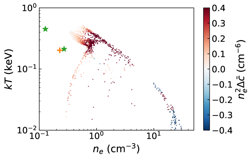
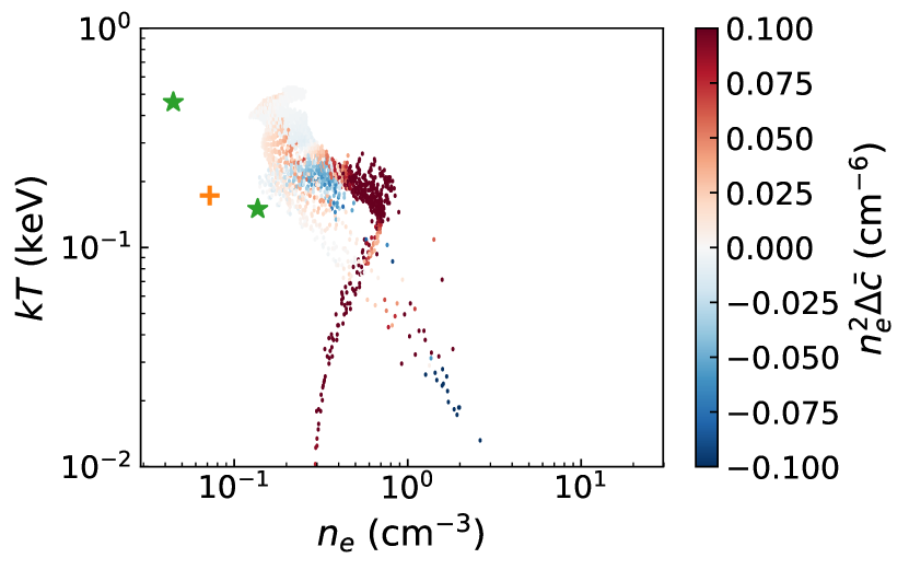
Figure 21: The phase diagrams of the projected regions of spectrum A (left) and spectrum B (right). The crosses show the fit parameters of the “vrnei” model; and the stars show the fit parameters of the two “vapec” model. The densities are underestimated as expected because of the assumption of filling factor (See the text).

From the simulation data, all the physical quantities (e.g. temperature, density, and ion fractions) can be used to obtain the true parameters underlying the fitted spectra. In Fig. 21, the phase diagrams of the real data for spectrum A and B show each region’s distinct evolution. The average charge difference is weighted by $n_{e}^{2}$ to more accurately capture each cell’s effect on the total emission. As these figures show, both the single- and two-temperature models have reasonable electron temperature values, given the breadth of the temperature distribution in the underlying region. The ionizing feature that is similar to the region “a” in Fig. 6 appears in both diagrams, because the ionizing shock front is always on the LOS. In the left panel, the phase diagram of spectrum A shows a clear line from top left to bottom right, similar to the iosbaric lines in Fig. 6. Both ionization and recombination appear in this line, which imply the thermal conduction could be the dominant process in these cells. In the right panel, the recombining gas is mainly situated in an area with a high temperature and low pressure, which is probably caused by adiabatic expansion.

Fig. 21 also shows that the best-fit densities are underestimated (as expected), and are about one tenth of the actual values. Thus the filling factor should be  0.32 instead of the assumed 1. In the left panel of Fig. 22, we plot the projected density within a range from $-9\,{\rm pc}$ to $-2\,{\rm pc}$ on the $z$-axis by averaging the density in this range along LOS. It shows the dense (non-X-ray-emitting) clouds in this thin slice of SNR. The spectrum A region is associated with a compressed cloud. In the right panel of Fig. 22, we plot the projected average density of hot gas ($T>1\times 10^{6}\,{\rm K}$). It averages the density in a range from $-30\,{\rm pc}$ to $30\,{\rm pc}$ on the $z$-axis. The bottom right spectrum B region is associated with a low density region.

Although both regions we selected for this example contain recombining plasma, the best-fit spectral models using diagnostics from oxygen alone only show that the gas has a broad temperature distribution. Real data obviously contrain lines from many more elements, which at the high spectral resolution provided by microcalorimeters will reveal both temperature and, we expect, ionization state information. We plan to do a next generation of simulations that will include all abundant elements and, we expect, indicate what analysis is needed to extract the time-dependent hydrodynamical parameters described in the main paper.

With the instruments on XRISM and Lynx, we can also produce simulated observations. We use the same regions as Athena to simulate spectra for the Lynx LXM. As the spatial resolution is much lower, a larger region (3′$\times$3′ box) was used for XRISM Resolve spectra. In Fig. 23, two example spectra are shown. They come from similar regions as the A and B spectra in Fig. 20 and can be fit to similar temperatures. The exposure time of every observation is 10$\,{\rm ksec}$ for both instruments. The future X-ray instruments have a higher spectral resolution which make it far easier to diagnose the RRC features as shown in the insert figure in the right panel. If the observed hot gas has an bulk motion on the LOS, the emission line will show a redshift, blueshift or broadening (See Hitomi Collaboration et al., 2016, for an example). The left panel shows the velocity dispersion of an OVIII line in the insert figure.

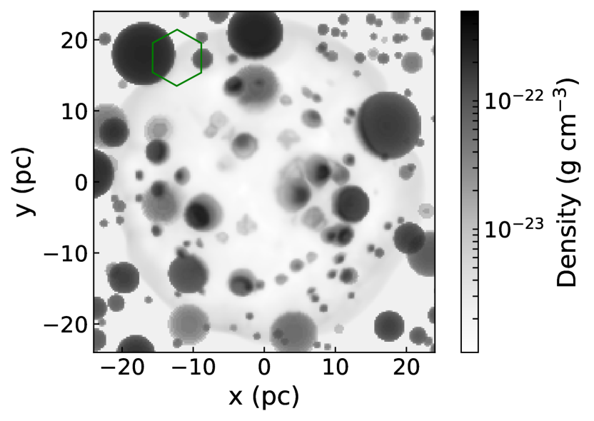
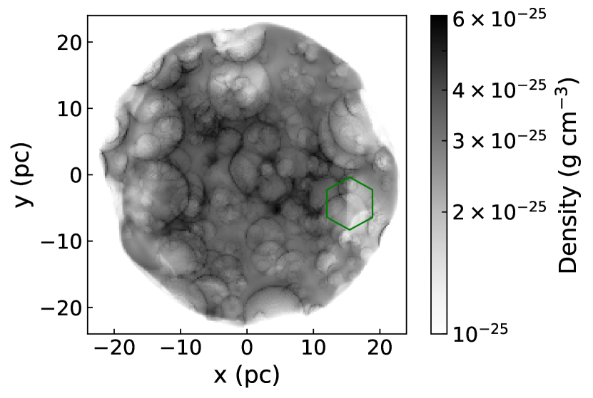
Figure 22: Left panel: projected average density along $z$-axis from -9 pc to -2 pc. Right panel: projected average density of X-ray emitting gas ($T>1\times 10^{6}\,{\rm K}$) along $z$-axis. The observation regions for Spectrum A and B in Fig. 19 are shown in green.

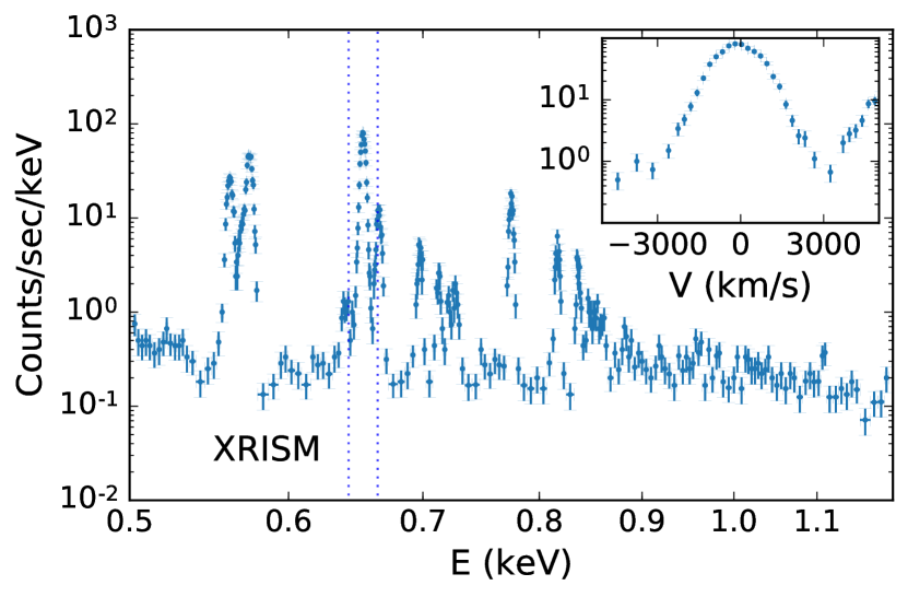
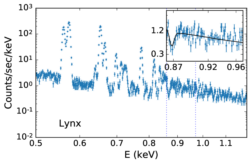
Figure 23: The example spectra from XRISM and Lynx. They are from regions similar to Spectrum A and B in Fig. 20 respectively. The XRISM spectrum (left panel) is extracted from a box of 3$\arcmin\times 3\arcmin$ around the spectrum A area. The insert figure in this panel shows the velocity dispersion of the strongest OVIII line with the range depicted as dotted lines in the spectrum. The Lynx spectrum (right panel) is extracted from a box of 1$\arcmin\times 1\arcmin$ in the spectrum B area. The insert image in this panel zooms in the RRC feature within the dotted lines.

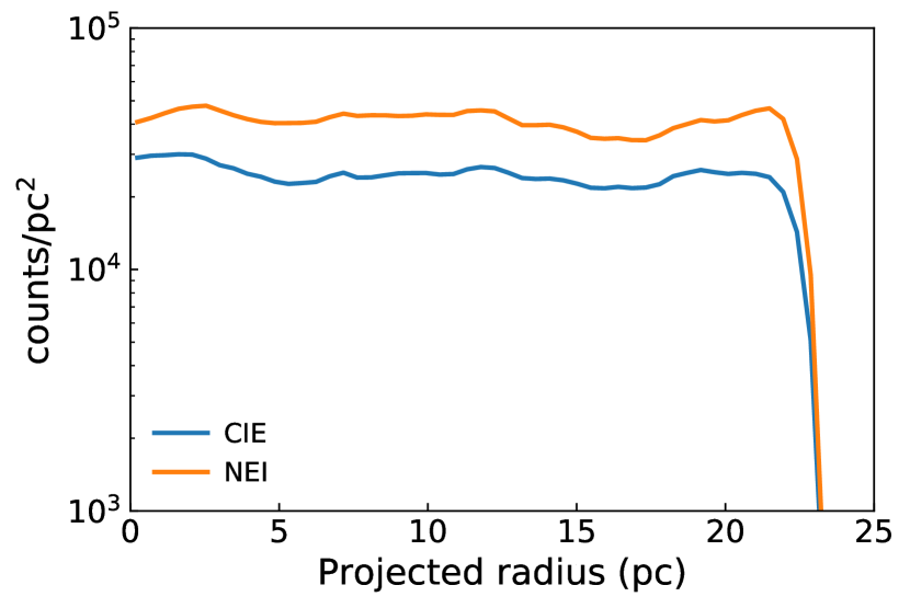
Figure 24: Surface brightness for the NEI and CIE for the same 3D simulation result (at 2$\times 10^{4}\,{\rm yr}$) with a shell thickness of 0.5 pc. The ions of hydrogen, helium, and oxygen are taken into account for the emission, and the energy range is 0.35 keV to 1.2 keV.

If we calculate the emission from the 3D simulation by assuming that it is in CIE at each pixel, results can also be generated from the same 3D simulation result. In Fig. 24, the surface brightness of NEI model is compared to the CIE assumption. The NEI model is about 30% brighter than CIE in this band. Both of them have a flat surface brightness in the interior of the SNR. In the shock front area, NEI model seems to have a brighter shell. When comparing to observations, other elements and energy ranges, omitted here, should of course also be included.

B.3 Connection between the $\Delta\bar{c}$ and the observed parameters

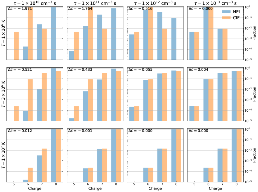
Figure 25: Ion fraction of oxygen (recombining from $T_{init}=1\times 10^{9}\,{\rm K}$) shown as a histogram. From top to bottom, electron temperature changes from $1\times 10^{6}\,{\rm K}$ to $1\times 10^{7}\,{\rm K}$; from left to right, the density-weighted timescale $\tau$ changes from $1\times 10^{10}\,{\rm cm}^{-3}\,{\rm s}$ to $1\times 10^{13}\,{\rm cm}^{-3}\,{\rm s}$. Only the ion fractions of which the charges are larger than 4 are shown in blue. The same ion fractions in equilibrium at corresponding temperatures are shown in orange as reference. The average charge differences defined in Equation (1) are labeled in each panel with three significant digits.

In our simulations, the average charge difference ($\Delta\bar{c}$) is used to show whether a cell is in an ionizing or recombining state and how far the NEI state is away from the equilibrium. In observations, however, it is more typical to fit an electron temperature ($T$), an initial temperature ($T_{init}$) and the density-weighted timescale ($\tau=n_{e}t$). To aid the observer, we show here the connection between $\Delta\bar{c}$ and $\tau$. Taking oxygen as an example, in Fig. 25, an initial temperature of 1$\times 10^{9}\,{\rm K}$ is used to show the recombination state with the temperature from $1\times 10^{6}\,{\rm K}$ to $1\times 10^{7}\,{\rm K}$ in three different ways. First, the ion fraction histograms of the NEI state (blue) and the CIE state (orange) can be compared to each other. They are calculated with the pyAtomDB (Foster et al., 2012). In an X-ray observation, the O⁶⁺ and O⁷⁺ ions that emit O VII and O VIII lines are the key ions, so we only show the high charge ions ($c>4$). We show the timescale $\tau$ on the top of each column. In the right most column, $\tau=1\times 10^{13}\,{\rm cm}^{-3}\,{\rm s}$, where the NEI is very close to the equilibrium. We also calculate $\Delta\bar{c}$ by using the ion fraction for each panel. From the ion fractions, when $|\Delta\bar{c}|<0.001$, the difference between the NEI state and the CIE state is small. Therefore, we use $\Delta\bar{c}<-0.001$ and $\Delta\bar{c}>0.001$ to determine of ionization and recombination respectively in our works to exclude the numerical fluctuation.

References

- Anders & Grevesse (1989) Anders, E., & Grevesse, N. 1989, Geochim. Cosmochim. Acta, 53, 197
- Barret et al. (2018) Barret, D., Lam Trong, T., den Herder, J.-W., et al. 2018, in Society of Photo-Optical Instrumentation Engineers (SPIE) Conference Series, Vol. 10699, Space Telescopes and Instrumentation 2018: Ultraviolet to Gamma Ray, 106991G
- Bell (2004) Bell, A. R. 2004, MNRAS, 353, 550
- Chandran & Maron (2004) Chandran, B. D. G., & Maron, J. L. 2004, ApJ, 602, 170
- Chen et al. (2008) Chen, Y., Seward, F. D., Sun, M., & Li, J.-t. 2008, ApJ, 676, 1040
- Cowie et al. (1981) Cowie, L. L., McKee, C. F., & Ostriker, J. P. 1981, ApJ, 247, 908
- Cox et al. (1999) Cox, D. P., Shelton, R. L., Maciejewski, W., et al. 1999, ApJ, 524, 179
- Foster et al. (2012) Foster, A. R., Ji, L., Smith, R. K., & Brickhouse, N. S. 2012, ApJ, 756, 128
- Fryxell et al. (2000) Fryxell, B., Olson, K., Ricker, P., et al. 2000, ApJS, 131, 273
- Greco et al. (2018) Greco, E., Miceli, M., Orlando, S., et al. 2018, A&A, 615, A157
- Harrus et al. (1997) Harrus, I. M., Hughes, J. P., Singh, K. P., Koyama, K., & Asaoka, I. 1997, ApJ, 488, 781
- Hitomi Collaboration et al. (2016) Hitomi Collaboration, Aharonian, F., Akamatsu, H., et al. 2016, Nature, 535, 117
- Ji et al. (2016) Ji, S., Oh, S. P., Ruszkowski, M., & Markevitch, M. 2016, MNRAS, 463, 3989
- John A. ZuHone et al. (2014) John A. ZuHone, Veronica Biffi, Eric J. Hallman, et al. 2014, in Proceedings of the 13th Python in Science Conference, ed. Stéfan van der Walt & James Bergstra, 103 – 110
- Jones et al. (1998) Jones, T. W., Rudnick, L., Jun, B.-I., et al. 1998, PASP, 110, 125
- Komarov et al. (2016) Komarov, S. V., Churazov, E. M., Kunz, M. W., & Schekochihin, A. A. 2016, MNRAS, 460, 467
- Lopez et al. (2013) Lopez, L. A., Pearson, S., Ramirez-Ruiz, E., et al. 2013, ApJ, 777, 145
- McKee & Cowie (1977) McKee, C. F., & Cowie, L. L. 1977, ApJ, 215, 213
- Miceli et al. (2010) Miceli, M., Bocchino, F., Decourchelle, A., Ballet, J., & Reale, F. 2010, A&A, 514, L2
- Nandra et al. (2013) Nandra, K., Barret, D., Barcons, X., et al. 2013, arXiv e-prints, arXiv:1306.2307
- Orlando et al. (2008) Orlando, S., Bocchino, F., Reale, F., Peres, G., & Pagano, P. 2008, ApJ, 678, 274
- Patnaude et al. (2009) Patnaude, D. J., Ellison, D. C., & Slane, P. 2009, ApJ, 696, 1956
- Patnaude & Fesen (2005) Patnaude, D. J., & Fesen, R. A. 2005, ApJ, 633, 240
- Petruk (2001) Petruk, O. 2001, A&A, 371, 267
- Rho & Petre (1998) Rho, J., & Petre, R. 1998, ApJ, 503, L167
- Shelton et al. (1999) Shelton, R. L., Cox, D. P., Maciejewski, W., et al. 1999, ApJ, 524, 192
- Slavin et al. (1993) Slavin, J. D., Shull, J. M., & Begelman, M. C. 1993, ApJ, 407, 83
- Slavin et al. (2017) Slavin, J. D., Smith, R. K., Foster, A., et al. 2017, ApJ, 846, 77
- Spitzer (1956) Spitzer, L. 1956, Physics of Fully Ionized Gases
- Suzuki et al. (2018) Suzuki, H., Bamba, A., Nakazawa, K., et al. 2018, PASJ, arXiv:1805.02882
- Turk et al. (2011) Turk, M. J., Smith, B. D., Oishi, J. S., et al. 2011, The Astrophysical Journal Supplement Series, 192, 9. http://stacks.iop.org/0067-0049/192/i=1/a=9
- Vink (2012) Vink, J. 2012, A&A Rev., 20, 49
- Vink & Laming (2003) Vink, J., & Laming, J. M. 2003, ApJ, 584, 758
- White & Long (1991) White, R. L., & Long, K. S. 1991, ApJ, 373, 543
- Yamaguchi et al. (2018) Yamaguchi, H., Tanaka, T., Wik, D. R., et al. 2018, ApJ, 868, L35
- Zhang & Chevalier (2018) Zhang, D., & Chevalier, R. A. 2018, ArXiv e-prints, arXiv:1807.06603
- Zhang et al. (2015) Zhang, G.-Y., Chen, Y., Su, Y., et al. 2015, ApJ, 799, 103
- Zhang et al. (2018) Zhang, G.-Y., Foster, A., & Smith, R. 2018, ApJ, 864, 79
- Zhou et al. (2016) Zhou, P., Chen, Y., Safi-Harb, S., et al. 2016, ApJ, 831, 192
- Zhou & Vink (2018) Zhou, P., & Vink, J. 2018, A&A, 615, A150
- Zhou et al. (2011) Zhou, X., Miceli, M., Bocchino, F., Orlando, S., & Chen, Y. 2011, MNRAS, 415, 244