Eigenvalue method for NEI unit in FLASH code

Abstract

We describe an improved non-equilibrium ionization (NEI) method that we have developed as an optional module for the FLASH magnetohydrodynamic simulation code. The method employs an eigenvalue approach rather than the earlier iterative ODE approach to solve the stiff differential equations involved in NEI calculations. The new code also allows the atomic data to be easily updated from the AtomDB database. We compare both the updated atomic data and the methods separately. The new atomic data are shown to make a significant difference in some circumstances, although the general trends remain the same. Additionally, the new method also allows simultaneous calculation of the non-equilibrium radiative cooling, which is not included in the original method. The eigenvalue method improves the calculation efficiency overall with no loss of accuracy. We explore some common ways to present the non-equilibrium ionization state with a sample simulation, and find that using average ionic charge difference from the equilibrium tends to be the clearest method.

1 Introduction

In astrophysical plasmas, the density can be so low that collisional interaction timescales can reach millions of years, leading to long delays between a thermodynamic event and eventual ionization equilibrium. In a collisional plasma, no ion population will be significantly impacted by a density-weighted timescale (fluence) less than $n_{e}t\sim 10^{7}\,{\rm cm}^{-3}\,{\rm s}$ and equilibrium is not reached until $\gtrsim 10^{12}\,{\rm cm}^{-3}\,{\rm s}$ (Smith & Hughes, 2010). Therefore, the widely-used astrophysical assumption of collisional ionization equilibrium (CIE) fails in many scenarios, and the impact of non-equilibrium ionization (NEI) must be considered. Beyond purely theoretical analysis, observations of supernova remnants (SNR; e. g., Zhang et al., 2015), intergalactic medium (e. g., Yoshikawa & Sasaki, 2006), and even possibly galaxy clusters (e. g., Prokhorov, 2010) have all shown NEI signatures in their X-ray spectra, including both ionizing and recombining features.

Magnetohydrodynamic (MHD) simulations can reproduce many astrophysical scenarios, likely to contain NEI plasmas, (such as SNR evolutions e. g., Zhou et al., 2011; Slavin et al., 2017), but the plasmas in the simulations are often assumed to be CIE due to the additional overhead and computations required by some NEI methods. If radiative cooling from heavy elements is significant in the MHD simulation or a detailed spectrum that can be compared to observations is one of the requirements of the simulation, the CIE assumption should be removed and an NEI calculation should be done along with the simulation.

Most current MHD simulation codes have not included the NEI calculation or the NEI unit is too slow for practical applications. To investigate how an astrophysical thermodynamic event influences the ionization states of the plasma, multi-dimensional MHD is required, which in turn requires the NEI calculation to be as fast as possible. With an improved simulation code and updated parameters, the NEI unit we show here will be more convenient to use for research involving collisional ionization in high energy astrophysics. One option, if radiative losses and gas mixing are not significant, is to approximate the effects after the initial MHD run. Shen et al. (2015) have developed a fast eigenvalue method that performs an NEI post-process analysis of MHD simulations without integrating the NEI into the simulation. The FLASH code (Fryxell et al., 2000) can perform the MHD simulation with an NEI unit in version 4.3 to calculate the change in the ion population with variations of the plasma’s density and temperature (Orlando et al., 2003). But the NEI unit in the code uses outdated ionization coefficients (Summers, 1974) and the current algorithm is inefficient. It uses a Bader-Deuflhard semi-implicit ODE solver (Bader & Deuflhard, 1983) to solve a sparse system of stiff linear equations with MA28. It assumes that during a hydro time step, the temperature and density remains unchanged and during the hydro process the advection of different species is independent from the ionization or recombination. The accuracy of this method is mainly determined by the accuracy of the atomic data (See a discussion in § 5.1). The radiative cooling is not considered in the original NEI unit which is important for most of UV to X-ray emitting hot gas.

In this paper, we describe an eigenvalue method for NEI in MHD simulations (§ 2), with comparisons to the existing method for consistency (§ 3). We update the atomic data in the original FLASH NEI code to use the updated rates (Bryans et al., 2009) from AtomDB (Foster et al., 2013) for comparison. In the eigenvalue method, a total radiative cooling from the plasma is also calculated (§ 4). Finally, a range of methods to measure the NEI states are discussed with examples (§ 5).

2 Eigenvalue method to solve the NEI problem

Masai (1984), Hughes & Helfand (1985), and Smith & Hughes (2010) described an eigenvalue method to calculate NEI evolution, which we briefly review below. For a given atomic species, the fraction of the $i$th ionization state can be derived from the differential equation set

$$\frac{\partial{F_{i}}}{\partial{t}}=n_{e}\big{\{}\alpha_{i-1}(T)F_{i-1}-[\alpha_{i}(T)+R_{i-1}(T)]F_{i}+R_{i}(T)F_{i+1}\big{\}}$$ (1)

where $n_{e}$ is the number density of electrons, $\alpha_{i}(T)$ is the ionization rate from state $i$ to state $i+1$, and $R_{i}(T)$ is the recombination rate from state $i+1$ to state $i$. This equation includes only single ionizations and two-body recombination. The method can be expanded, however, to include multiple ionization and three-body recombination, if desired. It can be written as a matrix equation,

$$\frac{\partial{}\bm{F}}{\partial{\tau}}=\bm{A}\cdot\bm{F},$$ (2)

where $\bm{F}$ is the ionization fraction vector for an atomic species, $\mathrm{d}\tau=n_{e}\mathrm{d}t$ is the time scale, and the tridiagonal matrix $\bm{A}$ contains the ionization rates and recombination rates as shown in equation (1).

In the numerical simulation, it can be assumed that the change of temperature and density can be neglected when the time step is small enough. For a given temperature $T$, the equilibrium fraction, the eigenvalues, and the eigenvectors of the matrix $\bm{A}$ are all constant, and thus can be precalculated. In the MHD run, as long as the temperatures remain within the allowable range, the corresponding equilibrium fraction can be found via interpolation by using the stored data tables. The eigenvalues and eigenvectors use the nearest temperature in the data tables (the accuracy of this interpolation is discussed in § 5.1).

The eigenvalue method can significantly accelerate the solution of differential equations, even though it requires more memory to store all the prepared constant vectors than other ordinary differential equation (ODE) solvers. Considering the equilibrium array, eigenvectors and eigenvalues matrix, about 0.4 MB more memory is required than the original method for all the twelve elements. It is worth mentioning that both original and eigenvalue method need memories to store the ions fractions in each cell. To make it accurate enough, the original ODE solver needed to modify the time step for solving the stiff equations. The eigenvalue method, however, provides an exact solution to the stiff equations as long as the temperature and density can be assumed to be constant within the time step. The accuracy depends only on how accurate the eigenvalues and eigenvectors are computed.

3 The neitest model in FLASH code

The NeiTest problem in FLASH code (v4.3) uses the NEI calculation unit to run a single test case. The test assumes that a plasma with a mass density of $2\times 10^{-16}\,{\rm g}\,{\rm cm}^{-3}$ flows with a constant uniform velocity of $3\times 10^{5}\,{\rm cm}\,{\rm s}^{-1}$ through a temperature jump going from $10^{4}\,{\rm K}$ to $10^{6}\,{\rm K}$. The plasma is in ionization equilibrium before going through the jump in the region at $T=10^{4}\,{\rm K}$.

We set up the simulation with the default parameters in one-dimension, running with 8 cpu cores using an Intel Fortran 2017 compiler. The results are recorded with an interval time of 50$\,{\rm s}$. The code stops when the time reaches 1000$\,{\rm s}$. The python-based yt-project (Turk et al., 2011) is used for the analysis of the results. The flow from lower temperature region to higher region can show the ionization along the time as the velocity is constant. After the “shock front” goes through the simulation regime, the ionization state at each point will become stable, which is not necessarily equilibrium. It is reasonable to use such a stable state to do post-process analysis. Considering the constant velocity and the largest spatial distance, it has become stable at $500\,{\rm s}$, and the result files can be used for the post process analysis. See Fig. 1 for the results for He ions as an example.

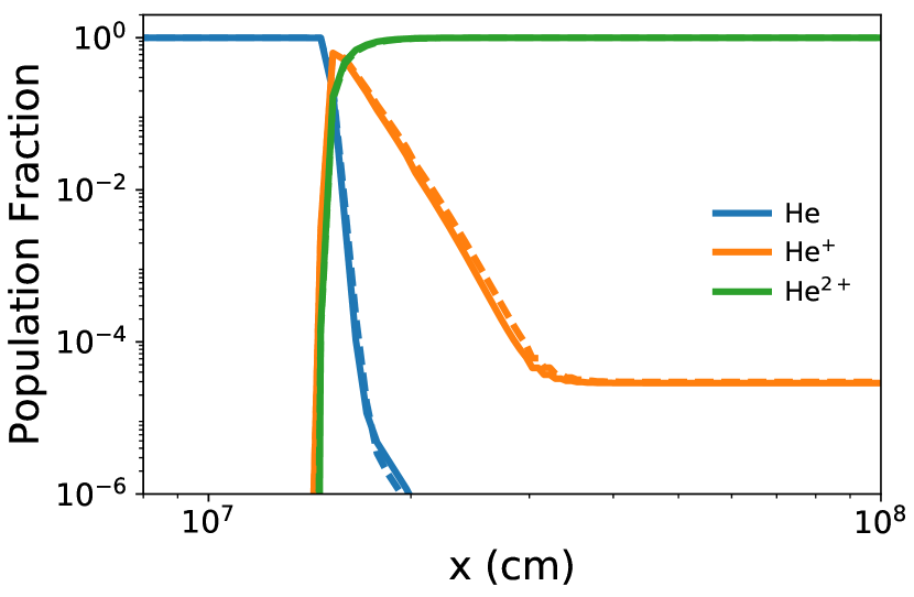
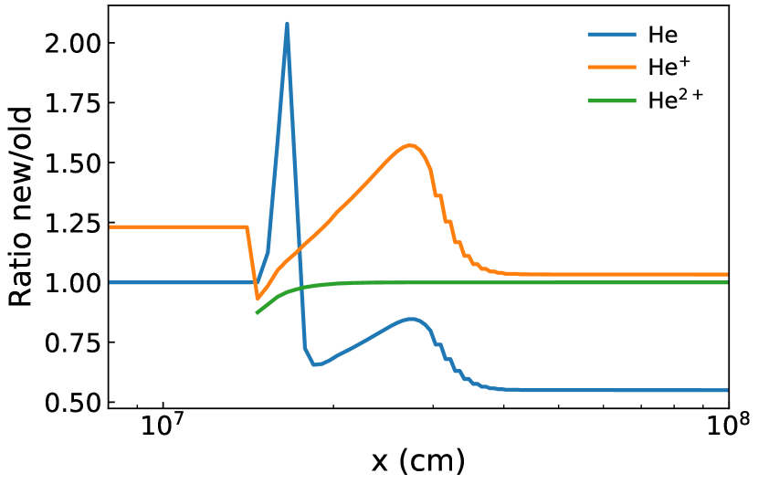
Figure 1: The population fractions evolution for He assuming a stationary flow through a temperature jump with the original ODE solver to compare the different ionization rate coefficients. Left panel: the result from the original ionization coefficients (solid lines) and the result from the new ionization coefficients (dashed lines). Right panel: the ratio of the results from the new ionization coefficients to the original one.

3.1 Impact of the updated atomic data

As mentioned in § 1, in the original NEI unit, a semi-implicit ODE solver to solve stiff equations is used for the evolution of ionization fractions. The table file “summers_den_1e8.rates” contains ionization and recombination rates for He, C, N, O, Ne, Mg, Si, S, Ar, Ca, Fe, Ni taken from Summers (1974). We substituted this file with one containing updated rates assembled by Bryans et al. (2009). All other parameters and settings are remained the same to allow comparison.

We have checked the differences for all the ions in the “summers_den_1e8.rates” file. Here, we only present the ratio between the updated one and the original one of He, O, and Si to show the differences (ignoring values below 1$\times 10^{-6}$). The results show that the new ionization coefficients can cause significant differences in the ionization test module (see Fig. 1 and Fig. 2). As expected, the overall trends for both the old and new ionization rate are the same. However, from the ratio figures, the ion fraction shows significant differences from the initial state to the final state, especially for heavier elements. This difference should be considered in the simulation or analysis of ionization in a plasma. In Fig. 2, we can see a “step” shape in lines, it is because FLASH code uses an adaptive mesh refinement (AMR) grid and the spatial resolution is not the same all over the simulation regime. It is sparser for a constant density on the right side.

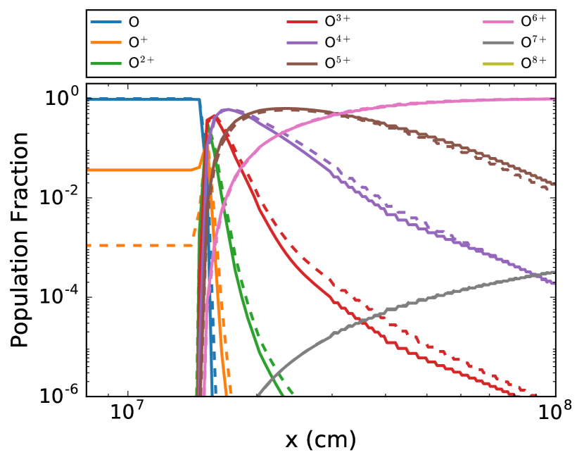
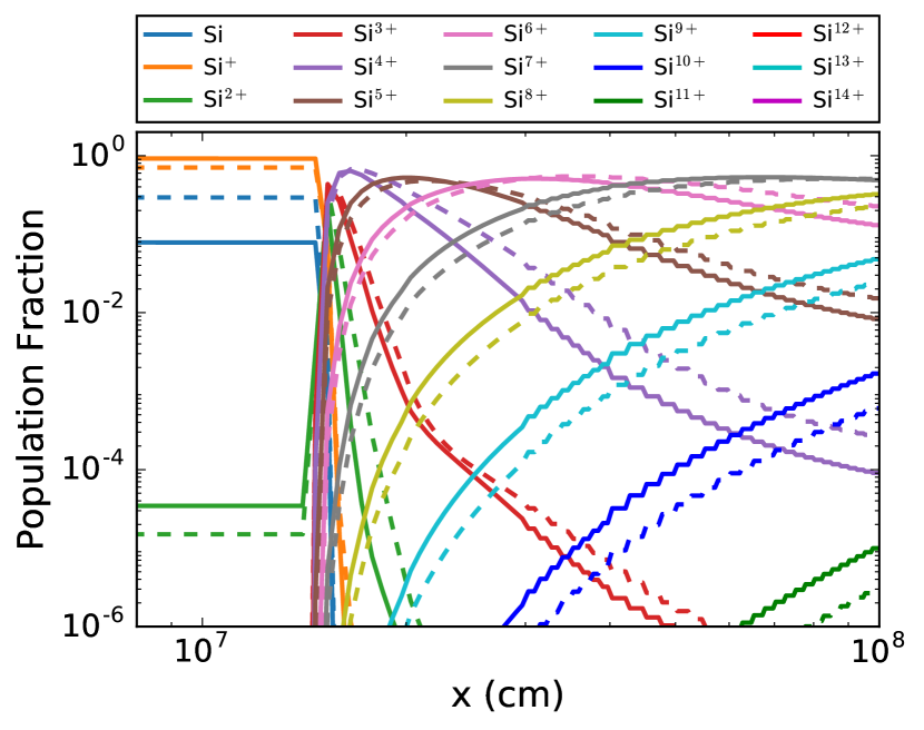
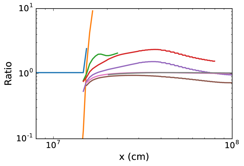
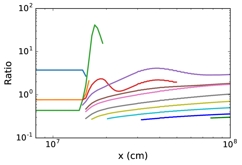
Figure 2: The population fractions ratios between the new atomic data and the original data for O (left) and Si (right) as examples. In the top panel, the result from the original ionization coefficients is displayed in solid lines and the result from the new ionization coefficients in dashed lines. Bottom panel is the ratio of the new to the original method coded in the same color as the top panel. It is not shown when the value for either method is less than $1\times 10^{-6}$.

3.2 Test the eigenvalue method

To compare the eigenvalue method with the original method, we also used the NeiTest simulation. The old ODE method code was run with the updated parameter table file as described in § 3.1, ensuring the codes are using the same atomic data.

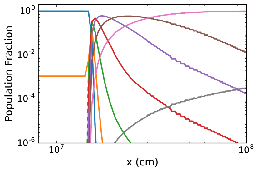
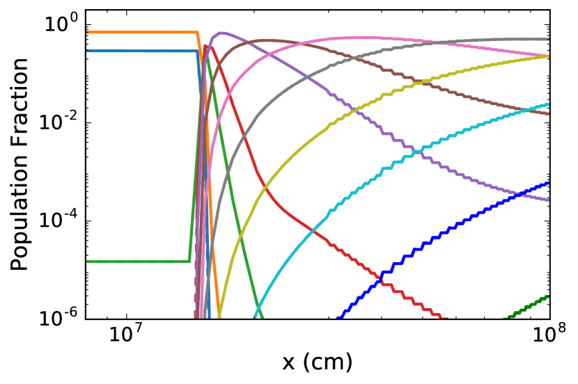
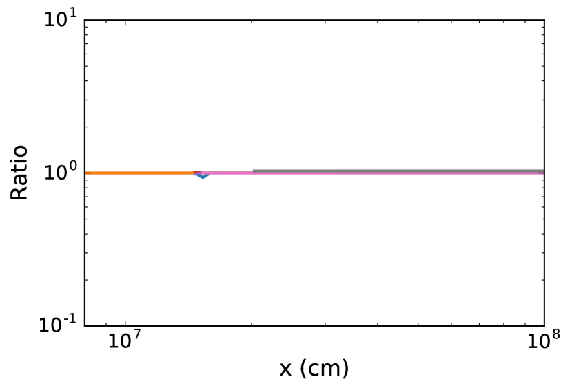
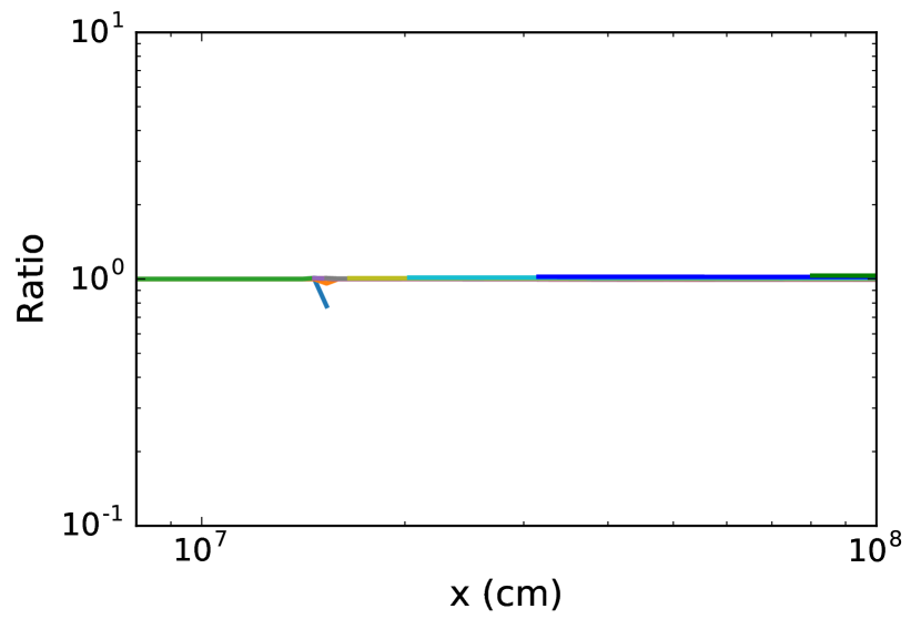
Figure 3: The comparison between the eigenvalue method and the standard ODE (MA28) method for O (left) and Si (right). The solid lines show the results from eigenvalue method; the dashed lines are from the original method (with the updated parameter table file). Bottom panel is the ratio of the new to the original method coded in the same color as the top panel. It is not shown when the value for either method is less than $1\times 10^{-6}$. All colors are coded the same with Fig. 2

In Fig. 3, the O and Si ions are shown as examples to compare the simulation results for the eigenvalue method and the original method used in the old NEI code. Because they use the same atomic data, the two methods are consistent with each other for the equilibrium state before and after the temperature jump. Beyond the jump, the values at very low populations differ slightly, mainly because these two methods use different thresholds for the lower limits on the fraction values. In the original method, a threshold of mass fraction is 1$\times 10^{-30}$; while in the eigenvalue method, a threshold of about $1\times 10^{-10}$ of ion fraction is used for the eigenvalues and eigenvectors. Therefore, the states of ions have a very small difference between each other. Considering the accuracy of the methods and the atomic data (See § 5.1), it is negligible. These ion populations with low values do not have much influence on the final results of the major population at that temperature.

To compare the performance of the eigenvalue method and the original method, two models were performed, “NeiTest” which is also the model used for the previous tests and a 2D parallel plane shock. The eigenvalue method needs to load the matrices to calculate the ionization in each cell, and this initialization process consumes more time than the original method. Table 1 has already separated the presentation of the “initialization” and “evolution” calculation time. For a larger simulation, “initialization” time can be neglected comparing to the whole simulation time. So we compare the “evolution” time of both methods here. By using a different number of threads for the same calculation, both methods provide an acceleration as more threads are used (See left panel of Fig. 4). The ratio between them remains similar for different number of threads. Because the FLASH code can use an AMR grid, the AMR refinement or the number of blocks of the simulation is another factor for the performance. With different size of fixed grids, the performance of both methods is compared in the right panel of Fig. 4 (four threads are used). Table 1 shows the results when the refinement level of AMR is free to change in a range from 1 to 6 for the two models. The plane shock model may change the block number as the shock front moving through the simulation box. From all the above tests, the eigenvalue method can be much more efficient than the original one (more than a factor of two.)

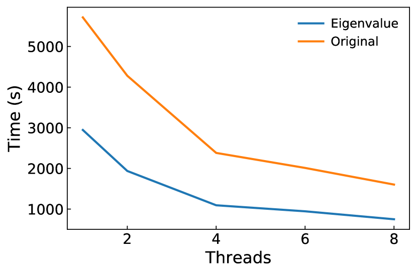
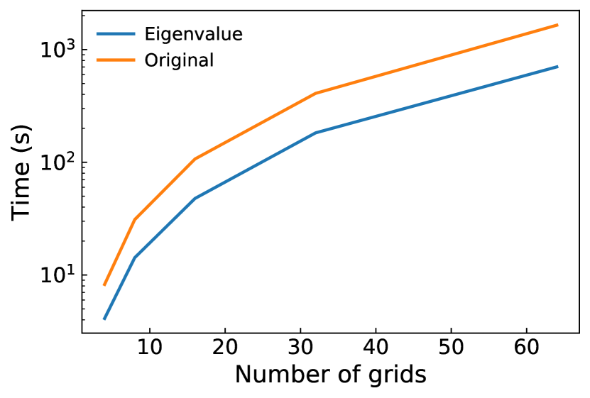
Figure 4: Consumed time (“evolution”) for different number of calculation threads (Left) and for different simulation grids (Right).

Table 1: NEI calculation performance

id	Model	Speedup	Eigenvalue Method			ODE (M28)
			Total time (s)	Initialization (s)	Evolution (s)	Total time (s)	Initialization (s)	Evolution (s)
1	NeiTest	1.67	104.105	2.942	101.158	172.575	0.113	172.458
2	NeiTest	1.67	103.192	2.992	100.197	172.516	0.146	172.366
3	NeiTest	1.67	103.309	2.996	100.309	172.486	0.140	172.342
4	NeiTest	1.68	99.828	2.859	96.965	168.298	0.140	168.154
5	Sod shock	2.51	131.129	6.462	124.634	329.777	1.470	328.777
6	Sod shock	2.49	130.873	6.544	124.414	326.245	1.469	324.740
7	Sod shock	2.52	130.911	6.544	124.332	330.040	1.455	328.553
8	Sod shock	2.55	131.434	6.533	124.869	335.459	1.518	333.894

4 Radiative cooling model

A radiative energy loss term has also been added to the NEI code, with a variable to switch it on and off. When it is switched on, the radiant energy density in unit time of each ion species (${s}_{rad}^{(z,i)}(T)$ in unit of $\rm{erg}\cdot\rm{cm}^{3}\cdot s^{-1}$) is retrieved from a database table based on the temperature. Here, $z$ and $i$ imply the atomic number and the ionization states respectively. Including the number densities and the volume, the energy loss rate is written as $\dot{u}_{rad}^{(z,i)}=\int s_{rad}^{(z,i)}\cdot n_{e}\cdot n_{z,i}\cdot dV$. Therefore, the total decrease on energy is the summation of every species $\Delta u=\sum\limits_{z}\sum\limits_{i}\dot{u}_{rad}^{(z,i)}\cdot\Delta t$. MHD codes such as FLASH are developed with an adaptive grid which makes it difficult to store the total energy. Instead, an energy variable in unit mass, $u_{m}=\Delta u/(\int\rho dV)$, can be used, which is also consistent with other energy variables in FLASH code. The mass density $\rho_{i}$ is connected to the number density of the species $n_{i}$ by $\rho_{i}=(\mu/N_{A})n_{i}$, where $\mu$ is the atomic weight of the species, $N_{A}$ is the Avogadro’s number. If it is for the whole gas, $\mu$ is the average atomic weight. The internal energy will subtract the energy loss at every step, and the temperature changes with the internal energy; the kinetic energy will then be impacted indirectly.

From the exponential results of eigenvalue method, $n_{z,i}$ can be calculated precisely during a hydro time step. With the integration, an exponential term ($(e^{\lambda_{i}n_{e}\Delta t}-1)/\lambda_{i}$) can be used instead of $\Delta t$. Currently we use the first-order approximation for a faster performance, and more importantly to make it an independent code unit that does not depend on the eigenvalue ionization calculation. It is a good estimation as long as the absolute value of $\lambda_{i}n_{e}\Delta t$ is small enough.

During the time step $\Delta t$ that is determined by the MHD evolution code (Courant-Friedrichs-Lewy; CFL condition), it is assumed that the temperature ($T$), the electron number density ($n_{e}$), and the fraction of each species that affects the ions’ number density ($n_{z,i}$) remain unchanged. When using the eigenvalue method, the calculation of ionization does not require a very small time step. However, the radiative cooling depends on and affects the temperature, density, and the variation of the ion fractions, which demand a time step small enough to make sure the energy loss can be assumed negligible. A new (smaller) time step will be required if the radiative loss exceeds a threshold. The new limit for time step is

$$\Delta t_{rad}=c_{rad}\frac{E_{int}}{|\Delta u|}\Delta t$$ (3)

where $\Delta t$ is the current time step, $E_{int}$ is the internal energy, and $c_{rad}$ is a constant to constrain the new time step. To be compatible with the CFL condition and make MHD simulation stable, $c_{rad}$ must be less than one. Although it can be adjusted to balance the requirement of accuracy and efficiency, we recommend a $c_{rad}$ less than 1$\times 10^{-2}$ to make sure that the first-order approximation and the assumption of an unchanged temperature within a time step are valid. The time step used by the simulation will chose the smallest value among the time steps determined by all physical conditions.

To test the radiative cooling model, a static simulation with a constant volume was performed with the initial temperature $T=1\times 10^{6}\,{\rm K}$, constant density $n_{H}=0.1\,{\rm cm}^{-3}$, and $c_{rad}=1\times 10^{-2}$. Fig. 5 shows that the results from the FLASH code and the same calculation of radiative cooling with python module (pyAtomDB). In the python calculation, the temperatures are directly adopted from FLASH code, but the ionization and emission energy rate are calculated from pyAtomDB.

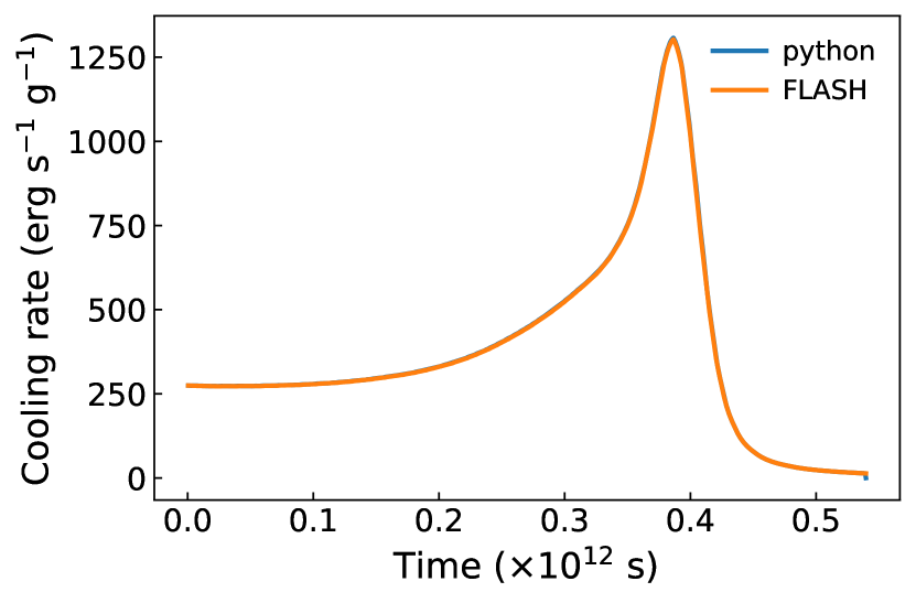
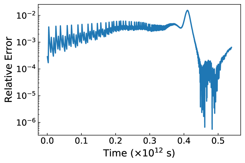
Figure 5: Cooling rate changes with time in a constant volume cell when the initial temperature is $1\times 10^{6}\,{\rm K}$ (Left), and the relative error correspondingly (Right).

The calculations are consistent with each other. When the cooling rate increases abruptly at about 4$\times 10^{11}\,{\rm s}$, temperature falls to 1$\times 10^{4}\,{\rm K}$ and the time step becomes smaller. We also perform several calculations with different initial temperatures. They show a similar or even smaller relative error. Because the NEI in the python scripts is calculated independently from the FLASH MHD simulation, we can also conclude that the NEI error does not accumulate. The range of the temperature for the radiative cooling is ($1\times 10^{4}\,{\rm K}$–$1\times 10^{9}\,{\rm K}$). The cooling process will not fail but print warnings if the temperature gets out of this range, because the data we use for the extended range of temperature are less accurate. As we focus on the X-ray emission here, the temperature range should be kept within this range.

5 Discussion

5.1 Accuracy of eigenvalue method

With the assumption that in a time step the temperature and density remain unchanged, the eigenvalue method is accurate no matter how large the time step is. However, there are some other sources of errors, such as the interpolation in temperature regime and the precision of the stored data. The precision can be made smaller by making sure the significant figures in the data are sufficient.

The interpolation is the main source of the inaccuracy here. From temperature $1\times 10^{4}\,{\rm K}$ to $1\times 10^{9}\,{\rm K}$, matrices of eigenvalues and eigenvectors for 5000 temperature nodes are generated. At a temperature node, the eigenvalue method with the matrices is accurate without error from interpolation. We also calculate the ionization cases at the 5000 temperature nodes with sparser matrices (1251 different temperature nodes) that is used in the new NEI unit of FLASH code. By comparing to the accurate results, the maximum of relative error ($|f_{1521}-f_{5000}|/f_{5000}$) is less than 5% throughout the temperature range. This was deemed acceptable considering that the error from atomic data (Dere, 2007) is about 10-15%, which is also true for the original ODE method. Therefore, currently the error for the NEI solution is mainly from the inaccuracy of the atomic data. A denser set of temperature matrices can be used to increase the accuracy when more accurate atomic data are available. We also tested the ionization cases with hundreds of steps and a big step covering the total time of small steps. The interpolation error does not accumulate.

5.2 Effect of the ionization of He

He is not a minority species. The ionization of He can affect both the electron density and the temperature even during a time step. When the temperature has been over $\sim 1\times 10^{5}\,{\rm K}$ for more than $n_{e}t\sim 10^{12}\,{\rm cm}^{-2}\,{\rm s}$, He will be essentially fully ionized and it will not change electron density and temperature. However, when the temperature is under $\sim 1\times 10^{5}\,{\rm K}$, the ionization or recombination of He can change the electron density by at most 20%. Ionization of He will also carry a fraction of energy from the hydrodynamic process, leading to a change in the temperature. The calculations relating to this temperature range or lower should be used carefully.

These effects will be added as a change of the electron density and a cooling procedure for ionization to the FLASH code in our future work. The same problem is even more severe with H that is assumed fully ionized in our simulations.

5.3 Methods to measure the ionization state

As a result from the stiff ODE, the difference between the NEI and equilibrium decreases exponentially, as the eigenvalues are negative. For an NEI plasma, we are generally interested in what kind of state (ionizing or recombining) the plasma is in, as well as the extent to which this state deviates from the equilibrium. We use results from an SNR simulation (taken from work in preparation) to display the effect of the different methods (Fig. 6). The simulation is set to be a SNR explosion going through some spherical dense clouds (in 2D; Slavin et al., 2017). The ionization and recombination appear in the shock front and around the clouds.

5.3.1 Ratio between two different ionization states

In many observations, the line emission ratios can be used to help determine the parameters in NEI models. For example, the line ratio between two different elements, two different ionization states of the same elements (Vasiliev, 2011), or the G-ratio and R-ratio of He-like triplet lines (Vink, 2012) can be used. The ratio between different elements is mainly determined by the abundances. The G and R-ratio also change with the ionization age. In our simulation code, we calculate the fractions of different ion states. Therefore, it is easier to calculate the line ratio between two ion states, such as $R=f(\rm{O}^{6+})/f(\rm{O}^{7+})$ (See an example in Fig. 6 middle left panel).

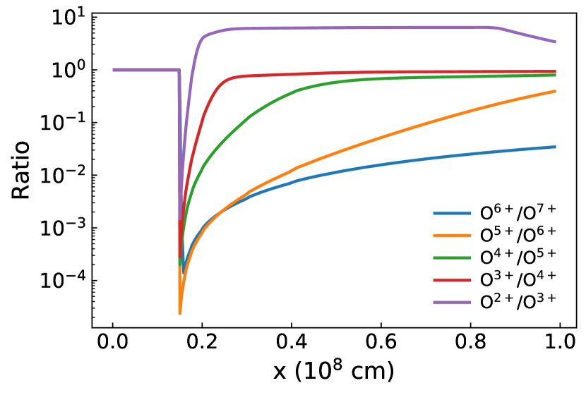
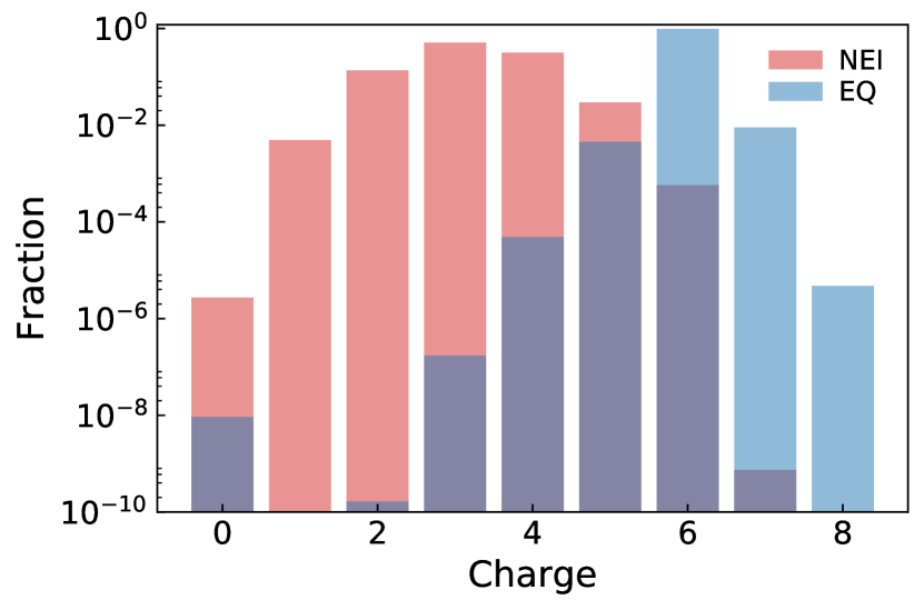
Figure 7: Left: The ratio $r_{b}=R_{eq}/R$ of different Oxygen ions for NeiTest simulation. Right: The distribution of oxygen ions in an ionizing state. Purple is the overlapping of red (NEI) and blue (equilibrium).

In a suitable temperature range, the ratio should represent the ionization states. The fraction ratio in the equilibrium to the NEI ratio ($r_{b}=R_{eq}/R$; $R_{eq}$ is the same fraction ratio of equilibrium) can be considered as a factor for the extent of the ionizing or recombining status. Assuming that the line fraction ratio can represent the temperature, this is a similar strategy used with the ionization balance temperature in the SPEX data analysis software (Kaastra et al., 1996). A recombining plasma should have $r_{b}>1$; an ionizing plasma should have $r_{b}<1$. However, the line ratio is not linear with temperature except over a narrow range, and different line ratios may show totally different results (See Fig. 7). The ratio between O²⁺ and O³⁺ in Fig. 7 shows a “recombining” feature because the ionization makes the distribution of the ion fraction move to higher ionization state. The proper ions must be carefully selected according to the temperature and ionization state to avoid such a false conclusion.

5.3.2 Average charge

The average charge can be defined by $C_{ave}=\sum\limits_{i=0}^{Z}f_{i}c_{i}$, where $f_{i}$ is the ion fraction with the fraction summation normalized to 1, $c_{i}$ is the charge for the ion, and $Z$ is the atomic number. It is assumed that ionization increases the average charge and recombination decreases it. Although in some dramatically turbulent plasma, the distribution can be multimodal (with more than one peak), and the ionizing and recombining may happen simultaneously, the average charge can still represent the overall tendency. Benjamin et al. (2001) even showed it could be used to approximate the entire NEI plasma states in certain circumstances.

Similar to the above case, the ratio of average charge between equilibrium and NEI $r_{c}=C_{ave,eq}/C_{ave}$ can be used to show the ionization state. The plasma is expected to be ionizing with $r_{c}>1$ or recombining with $r_{c}<1$. However, in a nearly neutral state, this ratio can be very sensitive to the small value in the denominator. In Fig. 6 middle right panel, some cold clouds are suggested to be in a “strong” recombination while other methods show less significance because of the small denominator effect.

Alternatively, the difference between the average charge in equilibrium and in NEI, $d_{c}=C_{ave,eq}-C_{ave}$, is similar to the ratio, $r_{c}$, with the critical value is 0 instead of 1. When $d_{c}$ is positive, the plasma is considered to be ionizing; when $d_{c}$ is negative, the plasma is considered to be recombining. It can also be written as $d_{c}=\sum\limits_{i=0}^{Z}(f_{eq,i}-f_{i})c_{i}$, which is charge-weighted deviation from equilibrium. In this case, the higher ionization states (which usually means a higher temperature) have more influence on this criteria (See Fig. 6 bottom-left panel for an example).

5.3.3 Timescale to achieve equilibrium

From the eigenvalue method, the solutions can be found from Appendix in Smith & Hughes (2010)

$${\bm{G}}=\sum\limits_{i=1}^{n}c_{i}e^{\lambda_{i}\tau}{\bm{V}_{R}}^{i}$$ (4)

indicating that the timescale ($n_{e}t$) can be represented by the $e$-folding time as $-1/\lambda_{i}$ (See Smith & Hughes, 2010, for the timescale-temperature relations), where $\lambda_{i}$ is the negative eigenvalue for the ion $i$. As the density ($n_{e}$) distribution can also be obtained from the simulation, the $e$-folding time ($t$) is depicted by $-1/(\lambda_{i}n_{e})$, which is dependent on the temperature and density. For a specific element, the maximum timescale that can be achieved with the maximum $\lambda_{i}$ implies how much fluence is required to get to equilibrium. However, with this method, the extent of closeness to equilibrium is determined without any information about whether the plasma is in an ionizing or recombining state. A combination of the timescale and the other methods are needed for showing the ionization states. In the bottom-right panel of Fig. 6, this timescale is shown for non-equilibrium (the absolute value of average charge difference is greater than $1\times 10^{-6}$) regions. The darker (time is larger) the map is, the further the NEI plasma is from achieving equilibrium.

5.3.4 Generating a spectrum

A spectrum with emission from all the ions of interest can be obtained from simulation results. This is the most direct way to compare with observations. With the relevant parameters for a specific telescope and instrument, we can mimic an “observed” spectrum. By fitting it, the detectable ionizing or recombining features and parameters, e.g. timescale, can be directly determined. But this approach requires more computing resources than all the previous methods, as a complete solution requires a 3D simulation and the projection of the 3D simulation. This method will be used and shown in a future work.

Except generating a spectrum, we recommend the average charge difference for the determination of an NEI state. In Fig. 8, we plot the density-temperature phase diagrams for the methods we mentioned above. All the pixels in the example simulation (Fig. 6) are shown in a scatter plot in the density-temperature plane that shows the average density and temperature in each MHD “pixel”. First, we can see that ion ratio is effective only for a special temperature range. Below about 6$\times 10^{5}\,{\rm K}$, the ratio of O⁶⁺ and O⁷⁺ is only a function of temperature. The “recombining” points in the lower temperature range are misleading. Some of them are in the shock front itself, where the temperature and ionization state are low but rapidly rising. In the top-right panel of Fig. 8, the average charge ratio is significant when the temperature is low and the average charges for both the ions state and the equilibrium are near to zero. To exclude the possibility of a zero-divided value, the average charge difference method is recommended for the depiction of ionization state. Sometimes only the ionizing or recombining states are important while how far it is from the equilibrium is not. Both the average charge ratio and average charge difference can satisfy the requirements with different critical values (1 and 0 respectively).

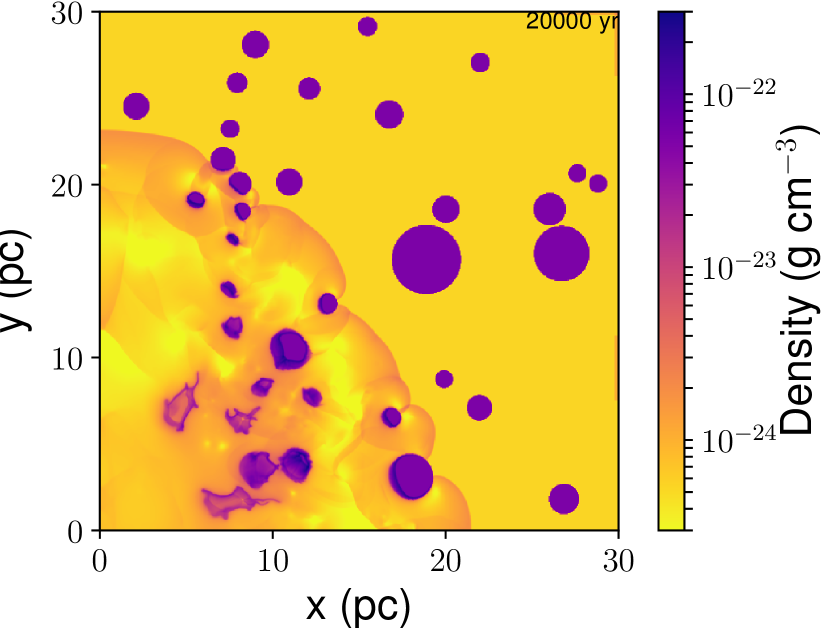
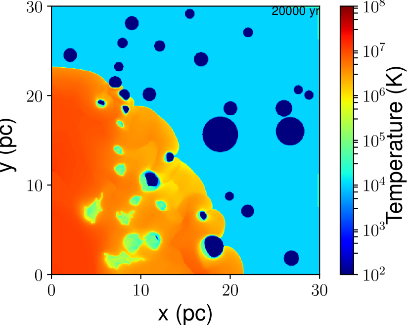
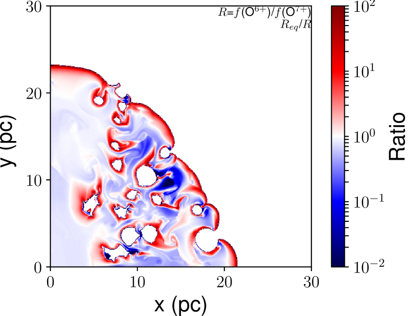
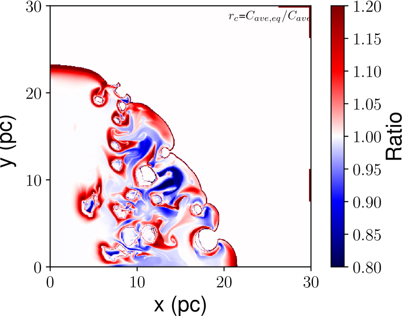
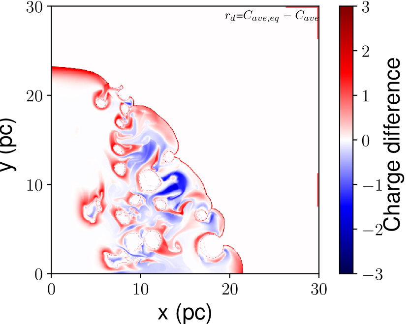
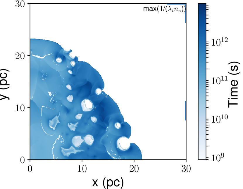
Figure 6: NEI indicators used in an example SNR simulation. Top-left: Density distribution; Top-right: Temperature distribution; Middle-left: ions ratio (See §5.3.1); Middle-right: average charge ratio (See §5.3.2); bottom-left: average charge difference (See §5.3.2); bottom-right: time for $e$-folding ionization/recombination (See §5.3.3).

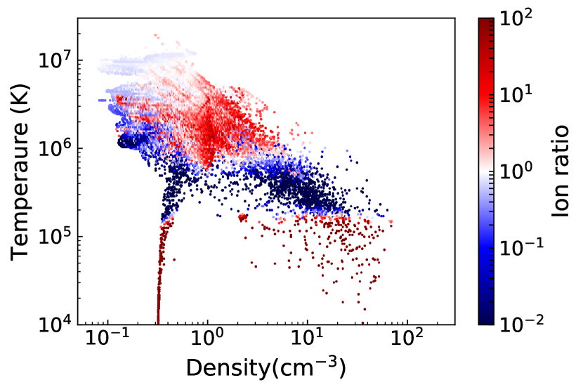
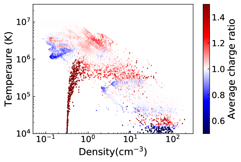
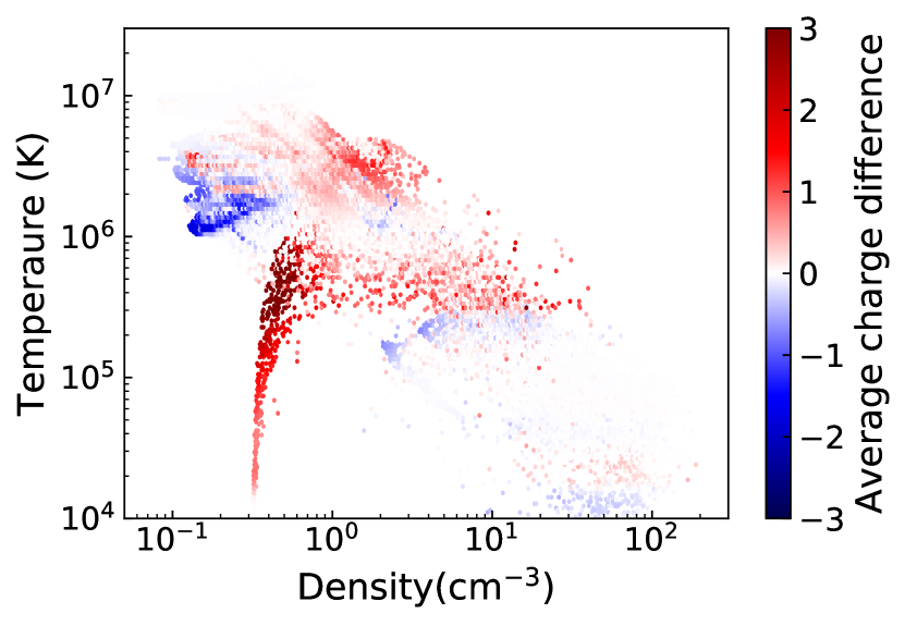
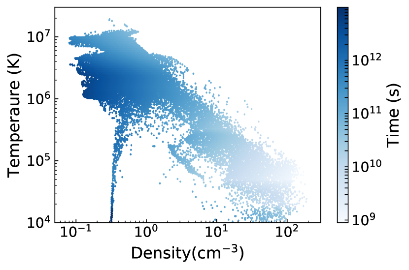
Figure 8: Density-temperature phase diagrams of the example simulation shown in Fig. 6. The four panels are correspondent to the lower four panels in Fig. 6 one by one, that is (from left to right, top to bottom) ions ratio of O⁶⁺ and O⁷⁺, average charge ratio, average charge difference, and the time of $e$-folding ionization/recombination.

5.4 NEI in Eulerian code

The FLASH code is primarily an Eulerian code. The NEI solver is separated from the FLASH hydrodynamic solver to get rid of the advection term in Eulerian fluid equation (See FLASH code manual § 16.2.1 for details). The ion fractions are firstly transported spatially without the “source” term (ionizing and recombining). After each transport step, an ordinary differential equation is solved in each cell with the elapsed time step, which is a first order approximation. In this version of the FLASH code (FLASH4), the particles in Lagrangian scheme can be used to trace the flow. The NEI code may be also used on the particles in a future work to see how it differs from the Eulerian code.

5.5 Applications to other MHD codes

Currently, the NEI calculation code is written in free-format Fortran code, compatible with the FLASH codes. For other MHD simulation code (e. g., ZEUS, ATHENA), the NEI calculation code can be compiled to a Fortran module to integrate with the MHD codes. The atomic data is stored in FITS files (Wells et al., 1981), and is available from AtomDB as a standard product at http://atomdb.org/download.php.

6 Summary

In this paper, we have described an optimized method, the eigenvalue method, to calculate NEI in an MHD simulation (FLASH code) with an updated atomic database. The updated database is compared with the original to show that the differences are large and the update is necessary. The new eigenvalue method is also compared to the original one by using the same updated database to show that the results are consistent to each other and the efficiency can be greatly improved. Radiative cooling of the ions used in the simulation can be included with the eigenvalue method in the simulation. We discussed the ways to measure the ionization states. With an example simulation, the average charge difference is shown as a better method.

References

- Bader & Deuflhard (1983) Bader, G., & Deuflhard, P. 1983, Numer. Math., 41, 373
- Benjamin et al. (2001) Benjamin, R. A., Benson, B. A., & Cox, D. P. 2001, The Astrophysical Journal Letters, 554, L225
- Bryans et al. (2009) Bryans, P., Landi, E., & Savin, D. W. 2009, ApJ, 691, 1540
- Dere (2007) Dere, K. P. 2007, A&A, 466, 771
- Foster et al. (2013) Foster, A. R., Ji, L., Yamaguchi, H., Smith, R. K., & Brickhouse, N. S. 2013, in American Institute of Physics Conference Series, Vol. 1545, American Institute of Physics Conference Series, ed. J. D. Gillaspy, W. L. Wiese, & Y. A. Podpaly, 252–259
- Fryxell et al. (2000) Fryxell, B., Olson, K., Ricker, P., et al. 2000, ApJS, 131, 273
- Hughes & Helfand (1985) Hughes, J. P., & Helfand, D. J. 1985, ApJ, 291, 544
- Kaastra et al. (1996) Kaastra, J. S., Mewe, R., & Nieuwenhuijzen, H. 1996, in UV and X-ray Spectroscopy of Astrophysical and Laboratory Plasmas, ed. K. Yamashita & T. Watanabe, 411–414
- Masai (1984) Masai, K. 1984, Ap&SS, 98, 367
- Orlando et al. (2003) Orlando, S., Peres, G., Reale, F., Rosner, R., & Siegel, A. 2003, Memorie della Societa Astronomica Italiana, 74, 643
- Prokhorov (2010) Prokhorov, D. A. 2010, A&A, 509, A29
- Shen et al. (2015) Shen, C., Raymond, J. C., Murphy, N. A., & Lin, J. 2015, Astronomy and Computing, 12, 1
- Slavin et al. (2017) Slavin, J. D., Smith, R. K., Foster, A., et al. 2017, ApJ, 846, 77
- Smith & Hughes (2010) Smith, R. K., & Hughes, J. P. 2010, ApJ, 718, 583
- Summers (1974) Summers, H. P. 1974, MNRAS, 169, 663
- Turk et al. (2011) Turk, M. J., Smith, B. D., Oishi, J. S., et al. 2011, The Astrophysical Journal Supplement Series, 192, 9
- Vasiliev (2011) Vasiliev, E. O. 2011, MNRAS, 414, 3145
- Vink (2012) Vink, J. 2012, A&A Rev., 20, 49
- Wells et al. (1981) Wells, D. C., Greisen, E. W., & Harten, R. H. 1981, A&AS, 44, 363
- Yoshikawa & Sasaki (2006) Yoshikawa, K., & Sasaki, S. 2006, PASJ, 58, 641
- Zhang et al. (2015) Zhang, G.-Y., Chen, Y., Su, Y., et al. 2015, ApJ, 799, 103
- Zhou et al. (2011) Zhou, X., Miceli, M., Bocchino, F., Orlando, S., & Chen, Y. 2011, MNRAS, 415, 244