Quasi-Bayes properties of a recursive procedure for mixtures

Sandra Fortini and Sonia Petrone
Bocconi University, Milan
Abstract

Bayesian methods are attractive and often optimal, yet nowadays pressure for fast computations, especially with streaming data and online learning, brings renewed interest in faster, although possibly sub-optimal, solutions. To what extent these algorithms may approximate a Bayesian solution is a problem of interest, not always solved. On this background, in this paper we revisit a sequential procedure proposed by Smith and Makov (1978) for unsupervised learning and classification in finite mixtures, and developed by M. Newton et al. (Newton and Zhang (1999)), for nonparametric mixtures. Newton’s algorithm is simple and fast, and theoretically intriguing. Although originally proposed as an approximation of the Bayesian solution, its quasi-Bayes properties remain unclear. We propose a novel methodological approach. We regard the algorithm as a probabilistic learning rule, that implicitly defines an underlying probabilistic model; and we find this model. We can then prove that it is, asymptotically, a Bayesian, exchangeable mixture model. Moreover, while the algorithm only offers a point estimate, our approach allows us to obtain an asymptotic posterior distribution and asymptotic credible intervals for the mixing distribution. Our results also provide practical hints for tuning the algorithm and obtaining desirable properties, as we illustrate in a simulation study. Beyond mixture models, our study suggests a theoretical framework that may be of interest for recursive quasi-Bayes methods in other settings.

Keywords. Asymptotic exchangeability. Bayesian nonparametrics. Conditionally identically distributed sequences. Dirichlet process. Predictive distributions. Recursive learning.

1 Introduction

Bayesian methods have always been attractive, for their internal coherence, their rigorous way of quantifying uncertainty through probability, their optimal properties in many problems. Analytic difficulties have been overcome by efficient computational methods and Bayesian procedures are nowadays widely and successfully used in many fields. However, fast computations remain a challenge, that hampers an even wider application of Bayesian methods among practitioners; the more so with streaming data and online learning, where inference and prediction have to be continuously updated as new data become available. In the modern trade off between information and computational efficiency, slightly misspecified but computationally more tractable methods receive renewed interest, as a reasonable compromise. Popular algorithms, such as Approximate Bayesian Computation (ABC) and variational Bayes, arise as approximations of an optimal Bayesian solution. Indeed, one could expect that a method which performs well is at least approximately Bayes. For a Bayesian statistician, the capacity of a learning scheme to be, at least approximately, a Bayesian learning scheme should be a minimal requirement for its validation.

This is the underlying theme of this paper, that we study and illustrate in a specific, important, case, namely sequential learning in mixture models. We revisit a recursive algorithm initially proposed by Smith and Makov (1978) for unsupervised sequential learning and classification in finite mixtures, and extended by M. Newton and collaborators (Newton et al. (1998), Newton and Zhang (1999), Quintana and Newton (2000), Newton (2002)), to provide a recursive fast approximation of the computationally expensive Bayesian estimate of the mixing density in nonparametric mixture models. Recent interesting developments are in Hahn et al. (2018). Convergence results have validated these algorithms as consistent frequentist estimators (Newton and Zhang (1999), Martin and Ghosh (2008), Ghosh and Tokdar (2006), Tokdar et al. (2009)). However, to what extend they provide an approximation of a Bayesian procedure, as for the original motivation, is not fully understood. In this paper we address this question, shedding light on their quasi-Bayes properties. Beyond mixture models, we believe that our results may offer a methodological viewpoint of interest for quasi-Bayes recursive computations in other settings.

Let us start by reminding the motivating problem in Smith and Makov (1978), sequential unsupervised learning and classification by mixtures. One wants to recursively classify observations $x_{1},x_{2},\ldots$ in one of $k$ populations (e.g., pattern types, or signal sources, etc.), with no feedback about correctness of previous classifications. A finite mixture model for this task assumes

$$X_{n}\mid\mathbf{\pi}\overset{i.i.d}{\sim}\sum_{j=1}^{k}\pi_{j}\;f_{j}(x).$$ (1)

Here the mixture components $f_{j}(\cdot)$ are known (extensive studies may be available on the specific components), but the mixing proportions $\mathbf{\pi}=(\pi_{1},\ldots,\pi_{k})$ are unknown. The classical Bayesian solution assigns a Dirichlet prior distribution on the unknown proportions, $\mathbf{\pi}\sim\text{Dir}(\alpha_{1},\ldots,\alpha_{k})$, and proceeds by Bayes rule. Learning is solved through the posterior distribution $p(\mathbf{\pi}\mid x_{1},\ldots,x_{n})$ and classification through the predictive probabilities that $X_{n+1}\sim f_{j},j=1,\ldots,K$, given $(x_{1},\ldots,x_{n})$. Unfortunately, computations, especially sequential computations, are involved.

The above model is a special case, with a discrete mixing distribution $\tilde{G}$ having atoms $1,\ldots,k$ and unknown masses $\pi_{1},\ldots,\pi_{k}$, of a general mixture model

$$X_{i}\mid\tilde{G}\overset{i.i.d}{\sim}f_{\tilde{G}}(x)=\int f(x\mid\theta)d\tilde{G}(\theta).$$ (2)

Here, a problem of interest is recursive estimation of the mixing distribution $\tilde{G}$. The mixture model (2) can be equivalently expressed in terms of a latent exchangeable sequence $(\theta_{i}$), such that the $X_{i}$ are conditionally independent, given $(\theta_{i})$, with $X_{i}\mid\theta_{i}\sim f(x\mid\theta_{i})$, and the $\theta_{i}$ are a random sample from $\tilde{G}$, that is, $\theta_{i}\mid\tilde{G}\overset{i.i.d}{\sim}\tilde{G}$. Then, the Bayesian estimate of $\tilde{G}$ with respect to quadratic loss, $E(\tilde{G}(\cdot)\mid x_{1},\ldots,x_{n})$, coincides with the predictive distribution $P(\theta_{n+1}\in\cdot\mid x_{1},\ldots,x_{n})$ of $\theta_{n+1}$ given the data. Thus, the problem can be rephrased as recursive prediction.

In a Bayesian nonparametric approach, a prior with large support is assigned on the random mixing distribution $\tilde{G}$; typically, a Dirichlet process (DP), with parameters $\alpha$ and $G_{0}$, $\tilde{G}\sim\text{DP}(\alpha,G_{0})$. DP mixtures have expanded in a floury of applications in many areas, and although many extensions have been developed, they remain a basic reference in Bayesian nonparametrics. Computational difficulties can be addressed by MCMC methods, or by variational Bayes or ABC approximations. If the observations $x_{i}$ arrive sequentially, one may resort to sequential Monte Carlo methods, sequential importance sampling (MacEachern et al. (1999)), or more recent sequential variational Bayes methods (Lin (2013), Broderick et al. (2013)), or combination of them (Christian A. Naesseth et al. (2018)). Still, these methods have a computational cost (for example, in the optimization steps), or only have a heuristic derivation; simple and fast recursive algorithms remain attractive.

Motivated by computations in DP mixture models, M. Newton and collaborators (Newton and Zhang (1999); Newton et al. (1998), Quintana and Newton (2000), Newton (2002)) proposed a simple recursive estimate for $\tilde{G}$, that starts at an initial guess $G_{0}$ and for $n\geq 1$ recursively computes the estimate

$$G_{n}(A)=(1-\alpha_{n})G_{n-1}(A)+\alpha_{n}\frac{\int_{A}f(x_{n}\mid\theta_{n})dG_{n-1}(\theta_{n})}{\int_{\Theta}f(x_{n}\mid\theta_{n})dG_{n-1}(\theta_{n})},$$ (3)

where $(\alpha_{n})$ is a sequence of real numbers in $(0,1)$ and it is usually assumed that $\alpha_{n}\rightarrow 0$ as $n\rightarrow\infty$, with $\sum_{n}\alpha_{n}=\infty$ and $\sum_{n}\alpha_{n}^{2}<\infty$. A standard choice, in analogy with DP mixtures, is $\alpha_{n}=1/(\alpha+n)$ with $\alpha>0$. For finite mixtures, as in (1), the rule (3) corresponds to the sequential procedure of Smith and Makov (1978).

Newton et al. (1998) propose the recursive rule (3) in applications to interval censored data and mixtures of Markov chains, further developed and extended, together with theoretical properties, by Newton and Zhang (1999). Theoretical properties have been studied from a frequentist viewpoint: that is, regarding $G_{n}$ as an estimator of the mixing distribution, under the assumption that the data are independent and identically distributed (i.i.d.) according to a true (identifiable) mixture model $f_{G_{true}}$. Smith and Makov (1978) prove frequentist consistency of their recursive estimator, for finite mixtures, using stochastic approximation techniques. Martin and Ghosh (2008) shed light on the connection with stochastic approximation, thus relating frequentist consistency of the algorithm to the convergence properties of stochastic approximation sequences. They prove consistency of $G_{n}$ for a discrete $G_{true}$ with known atoms, and extend to the case of mixture kernels with an unknown common parameter. Ghosh and Tokdar (2006) and Tokdar et al. (2009) prove frequentist weak consistency of the estimator (3), under conditions on the mixture kernels, and give results on convergence in probability for a permutation-invariant version of it.

Again, these results regard Newton’s algorithm (3) as a frequentist estimator. Its theoretical properties as an approximation of the computationally expensive Bayesian solution remain quite unsolved. One could argue that, when consistent, Newtons’ estimator will asymptotically agree, almost surely with respect to the law of i.i.d. observations from a true $F_{G_{true}}$ ($F_{G_{true}}^{\infty}$-a.s.), with a consistent Bayesian estimator for $\tilde{G}$. But, also, with any other consistent estimator for $\tilde{G}$; which flattens their different nature. These results are important, and Newton’s recursive estimator has the advantage of being computationally faster than other consistent estimators for the mixing distribution; but its Bayesian motivation is lost.

We take another, we believe more properly Bayesian, approach. Our starting point is that, when using (3), a researcher is changing the learning rule on $\theta_{n+1}$; therefore, implicitly, using a probabilistic model that is different from the Bayesian exchangeable model (2). What is this model? Is it quasi-Bayes? This remark potentially applies to other approximation algorithms which, as well, more or less implicitly, use a probabilistic model different from the stated Bayesian one.

To address these questions, we need to formalize a notion of a quasi-Bayes procedure. The term quasi-Bayes is used under many meanings in the literature (see e.g. Li et al. (2018)). We mutuate this term from Smith and Makov (1978), and formalize its meaning as follows. Details are given in Section 3. Mixture models specify an exchangeable probability law for the infinite sequence $(X_{n})$. A quasi-Bayes learning rule for mixtures should preserve this invariance property, at least asymptotically. This holds more generally, beyond mixture models. A first requirement we ask for a probabilistic learning rule to be a quasi-Bayes approximation of a Bayesian exchangeable learning rule is asymptotic exchangeability. Informally, the observations’ labels do not matter if we look at far enough pieces of the sequence $(X_{n})$. Yet, asymptotic exchangeability is only a minimal property. A refinement refers to a specific exchangeable law. Let ${\tilde{P}}$ be an exchangeable probability law for $(X_{n})$. We say that $P$ is a quasi-Bayes approximation of ${\tilde{P}}$ if it is asymptotically exchangeable, and the exchangeable limit sequence has probability law ${\tilde{P}}$.

On this basis, we address the following questions:

1. If a researcher uses the recursive procedure (3) as a probabilistic learning rule, that is, she uses (3) as the predictive distribution for the latent parameter $\theta_{n+1}$, given $x_{1:n}$, what probabilistic model is she implicitly assuming for the observable $(X_{n})$? Is it an approximation, at least asymptotically, of a Bayesian, exchangeable, mixture model?

We prove that the probabilistic model underlying the recursive rule (3) is indeed asymptotically exchangeable. More precisely, it implies that the sequence $(X_{n})$ is conditionally identically distributed (c.i.d.) (Kallenberg (1988), Berti et al. (2004)); roughly speaking, for any $n$, future observations $X_{n+k},k\geq 1$, are identically distributed, given $X_{1:n}$. For stationary sequences, the c.i.d. property is equivalent to exchangeability; in general, a c.i.d. sequence is not exchangeable, but it is such asymptotically. This first result says that a researcher using (3) as the predictive rule is implicitly assuming some form of non stationarity in the data, that tends to vanish in the long run. A c.i.d. model could actually be the appropriate model in situations where exchangeability is broken by competition, selection or other forms of non stationarity, but the system converges to a stationary, exchangeable steady state. If, instead, it is used as an approximation of a honest exchangeable model, it guarantees the minimal property of being asymptotically exchangeable: $(X_{n+1},X_{n+2},\ldots)$ converge in distribution to an exchangeable sequence, say $(Z_{n})$. See Section 3.

Asymptotic exchangeability alone does not explicitly provide the statistical model of the limit sequence $(Z_{n})$; which is also, by the above result, the asymptotic statistical model for the c.i.d. sequence $(X_{n})$. We thus refine the result by finding such model. Namely, we prove that there exist a random distribution $G$, which is the almost sure weak limit of the sequence $G_{n}$, such that the $Z_{n}$ are conditionally i.i.d. given $G$, according to a distribution $F_{G}$ with density $f_{G}$ of the form (2). Therefore, so are the $X_{n}$, asymptotically; roughly speaking, $X_{i}\mid G\overset{iid}{\approx}F_{G}$ for $n$ large, where $\overset{iid}{\approx}$ means approximately i.i.d. In this sense, Newton’s recursive learning rule arises from a quasi-Bayes mixture model.

These results shed light on an open question by Martin and Ghosh (2008). Although Newton’s recursive rule is motivated by computations in DP mixture models, they show two examples where the Bayesian estimate of $G$ with a DP prior and the recursive estimate $G_{n}$ have different performance. Thus, they pose an open question: If Newton’s recursive algorithm is not an approximation of the DP prior Bayes estimate, for what prior does the recursive estimate approximate the corresponding Bayes estimate? Our results explain the reason why the random distribution $G$ may have a probability law far apart from a DP. The recursive rule (3) underlies a sequence $(\theta_{n})$ which is not exchangeable; thus, there is no random mixing distribution $G$ such that $\theta_{i}\mid G\overset{i.i.d}{\sim}G$ (one might rather think, in a state-space fashion, of a sequence of random distributions $\tilde{G}_{n}$, such that $\theta_{n}\mid\tilde{G}_{n}\overset{indep}{\sim}\tilde{G}_{n}$; see Section 3). However, we show that such $G$ exists asymptotically, and $\theta_{n}\mid G\overset{iid}{\approx}G$ for $n$ large. The probability law of $G$ (“the prior”) is implicitly determined by the c.i.d. sequence $(X_{n})$, through its so-called directing random measure $F_{G}$; and, if the mixture $F_{G}$ is identifiable, it is unique. (Notice that we are denoting with the same symbol a distribution function (d.f.) and the corresponding measure). Results on the explicit law of the directing random measure of c.i.d. sequences are known only in limited, simple cases. We do obtain that the directing random measure for $(X_{n})$ is a mixture of the form $F_{G}$, but we do not have explicit results on the distribution of $G$. However, we can prove that, under fairly mild conditions, the random distribution $G$ is absolutely continuous, a.s.; thus, its law is rather a smoothing of a Dirichlet process, the latter a.s. selecting discrete distributions. In fact, Newton’s algorithm was originally given in terms of densities, assuming that the unknown mixing distribution is absolutely continuous, with density $g$. Notice that, if $G_{0}$ is absolutely continuous with respect to a sigma-finite measure $\lambda$ on $\Theta$ (denoted $G_{0}\ll\lambda$), then also $G_{n}\ll\lambda$, a.s., for every $n\geq 1$, and its density $g_{n}$ satisfies the recursive equations

$\displaystyle g_{n}(\theta)$ $\displaystyle=(1-\alpha_{n})g_{n-1}(\theta)+\alpha_{n}\frac{g_{n-1}(\theta)f(x_{n}\mid\theta)}{\int f(x_{n}\mid\theta^{\prime})g_{n-1}(\theta^{\prime})d\lambda(\theta^{\prime})}.$ (4)

We have given Newton’s rule (3) for the distributions, as they are better defined objects when we read the algorithm as a probabilistic learning rule.

2. The second main question we address is as follows. As an algorithm, Newton’s recursive rule (3) only gives a point estimate of the mixing distribution $G$. Can one provide a more complete description of the uncertainty? A Bayesian approach would fully describe the uncertainty through the posterior distribution. Can one enrich Newton’s algorithm, by providing a posterior distribution on $G$?

Our key to address this question is, again, to regard Newton’s rule (3) as a probabilistic learning rule. We can then formally prove that $G_{n}(\cdot)=E(G(\cdot)\mid x_{1},\ldots,x_{n})$, thus, it is, indeed, the point estimate of $G$ under quadratic loss; moreover, although the prior distribution of $G$ is only implicitly defined, we can approximate the posterior distribution of $G$, that results from such implicit prior. More specifically, we provide convergence rates and an asymptotic Gaussian approximation of the finite dimensional conditional distribution $P([G(A_{1}),\ldots,G(A_{k})]\in\cdot\mid x_{1},\ldots,x_{n})$, for any fixed measurable sets $A_{1},\ldots,A_{k}$, $k\geq 1$. Thus, not only one has a quasi-Bayes point estimate, but may provide asymptotic credible regions.

These results illuminate on the probabilistic model implied by Newton et al.’s recursive rule. Interestingly, this understanding also gives new insights on the role of the weights $\alpha_{n}$ and of other main parameters of the model. As we illustrate in Section 5, it provides practical advise about tuning the algorithm for obtaining desirable properties; notably, for attenuating the effect of the lack of exchangeability on the estimates, a problem usually addressed, with higher computational cost, by taking averages over permutations of the sample.


Section 2 recalls the basic structure of DP mixture models, and introduces our viewpoint on Newton et al.’s recursive algorithm as a probabilistic learning rule. We prove its quasi-Bayes properties in Section 3. Section 4 provides rates and asymptotic results, together with asymptotic credible intervals. A simulation study for location mixtures of Gaussian distributions, in Section 5, illustrates how the undesirable sensitivity of the estimates to the ordering of the observation can be attenuated, by tuning the weights and the main parameters of the model. All the proofs are collected in Section 6. Directions for developments are finally discussed.

2 Dirichlet process mixtures and a new look at Newton’s sequential procedure

We first recall the basic structure of Bayesian inference for DP mixture models, in order to motivate in more details the recursive rule (3), and to introduce some further notation.

Again, the DP mixture model has a hierarchical formulation in terms of a latent exchangeable sequence $(\theta_{i})$

$\displaystyle X_{i}\mid\theta_{i}\overset{indep}{\sim}f(x\mid\theta_{i})$ (5)
$\displaystyle\theta_{i}\mid\tilde{G}\overset{i.i.d}{\sim}\tilde{G},$
$\displaystyle\tilde{G}\sim\text{DP}(\alpha G_{0}),$

where (5) is a short notation for $X_{n}\mid X_{1},\dots,X_{n-1},(\theta_{n})\sim f(x\mid\theta_{n})$, for every $n\geq 1$, and $f(\cdot\mid\theta)$ is a density with respect to a sigma-finite measure $\mu$ on the sample space $\mathbb{X}$. Integrating the $\theta_{i}$ out, one has the mixture model (2), with a DP prior on $\tilde{G}$. We denote by ${\tilde{P}}$ the probability law on the process $((X_{n},\theta_{n}))$ so defined. We assume that the $X_{i}$ and the $\theta_{i}$ are, respectively, random variables with values in $\mathbb{X}\subseteq\mathbb{R}^{d}$ and $\Theta\subseteq\mathbb{R}^{p}$, equipped by their Borel sigma-fields $\mathcal{B}(\mathbb{X})$ and $\mathcal{B}(\Theta)$; but the results hold more generally, for Polish spaces. Throughout the paper, we refer to conditional distributions as regular versions. We use the short notation $X_{1:n}=(X_{1},\ldots,X_{n})$, and $P(A\mid x_{1:n})$ for $P(A\mid X_{1}=x_{1},\ldots,X_{n}=x_{n})$. Unless explicitly stated, convergence of distributions is in the topology of weak convergence. Weak convergence of $F_{n}$ to $F$ is denoted by $F_{n}\Rightarrow F$.

Inference on $\tilde{G}$ in a DP mixture model moves from the conditional distribution

$$\tilde{G}\mid\theta_{1:n},x_{1:n}\sim\text{DP}(\alpha G_{0}+\sum_{i=1}^{n}\delta_{\theta_{i}}),$$

to get the posterior distribution as a mixture of DPs

$$\tilde{G}\mid x_{1:n}\sim\int\text{DP}(\alpha G_{0}+\sum_{i=1}^{n}\delta_{\theta_{i}})\,d{\tilde{P}}(\theta_{1:n}\mid x_{1:n}).$$ (6)

The Bayesian point estimate $\tilde{G}_{n}^{(Bayes)}$ of $\tilde{G}$, with respect to quadratic loss, is the conditional expectation of $\tilde{G}$, and coincides with the predictive distribution of $\theta_{n+1}$, given $X_{1:n}$. By the Pólya urn structure characterizing the Dirichlet process

$${\tilde{P}}(\theta_{n+1}\in\cdot\mid\theta_{1:n},x_{1:n})=\frac{\alpha G_{0}(\cdot)+\sum_{i=1}^{n}\delta_{\theta_{i}}(\cdot)}{\alpha+n},$$ (7)

therefore

$\displaystyle\tilde{G}_{n}^{(Bayes)}(\cdot)$ $\displaystyle=$ $\displaystyle E(\tilde{G}(\cdot)\mid x_{1:n})={\tilde{P}}(\theta_{n+1}\in\cdot\mid x_{1:n})\quad\quad$
$\displaystyle=$ $\displaystyle\frac{\alpha G_{0}(\cdot)+\sum_{i=1}^{n}{\tilde{P}}(\theta_{i}\in\cdot\mid x_{1:n})}{\alpha+n}$
$\displaystyle=$ $\displaystyle\frac{\alpha+n-1}{\alpha+n}\,\frac{\alpha G_{0}(\cdot)+\sum_{i=1}^{n-1}{\tilde{P}}(\theta_{i}\in\cdot\mid x_{1:n})}{\alpha+n-1}+\frac{1}{\alpha+n}{\tilde{P}}_{\tilde{G}_{n-1}^{Bayes}}(\theta_{n}\in\cdot\mid x_{n}),$

where

$${\tilde{P}}_{\tilde{G}_{n-1}^{(Bayes)}}(\theta_{n}\in A\mid x_{n})=\frac{\int_{A}f(x_{n}\mid\theta)d\tilde{G}_{n-1}^{(Bayes)}(\theta)}{\int_{\Theta}f(x_{n}\mid\theta)d\tilde{G}_{n-1}^{(Bayes)}(\theta)}.$$ (9)

In the Bayesian estimate, as a new observation $x_{n}$ becomes available, the information on all the past $\theta_{i},i=1,\ldots,n-1$, is updated. This efficiently exploits the sample information, but is computationally expensive. Instead, Newton’s algorithm (3) does not update the estimate $G_{n-1}$, and $x_{n}$ only enters in inference on $\theta_{n}$, in an empirical Bayes flavor. The two estimates coincide only for $n=1$. However, even for $n=1$, Newton’s rule makes a simplification of the posterior distribution of $G$, replacing the mixture of Dirichlet processes $\int\text{DP}(\alpha G_{0}+\delta_{\theta_{1}})d{\tilde{P}}(\theta_{1}\mid x_{1})$, as from (6), with a DP ($\alpha G_{0}+{\tilde{P}}(\theta_{1}\mid x_{1}))$. For $n\geq 1$, Newton’s estimate loses in efficiency, not fully exploiting the sample information, but, on the other hand, is very fast; if one evaluates (3) on a grid of $m$ points and calculates the integral that appears at the denominator using, say, a trapezoid rule, then the computational complexity is $mn$.

2.1 Newton’s algorithm as a probabilistic learning rule

As underlined, in DP mixture models, the point estimate $E(\tilde{G}\mid x_{1:n})$ corresponds to the predictive distribution of $\theta_{n+1}\mid x_{1:n}$. Our point is that, similarly, Newton’s recursive rule should be regarded as a probabilistic learning rule for model (5), that expresses a different, computationally simpler, predictive distribution for the $\theta_{n}$:

$$\begin{array}[]{cc}X_{n}\mid\theta_{n}\overset{indep}{\sim}f(x\mid\theta_{n})\\ \theta_{n+1}\mid x_{1:n}\sim G_{n}(\cdot),\;n\geq 1,\end{array}$$ (10)

with $\theta_{1}\sim G_{0}$ and $G_{n}$ given by (3).

A known result in probability theory is that the predictive rule for a sequence of random variables characterizes the probability law of the sequence (Ionescu-Tulcea Theorem). On this basis, a researcher using the predictive rule (3) is implicitly using a different probabilistic model for the sequence $((X_{n},\theta_{n}))$, in place of the exchangeable mixture model (2). Our aim is to make this model explicit. Such model may be of autonomous interest in some experimental circumstances. When we regard Newton’s sequential procedure as a probabilistic learning rule, it provides the formal framework for understanding its quasi-Bayes properties.

Let us denote by $P$ a probability law on $((X_{n},\theta_{n}))$ that is consistent with assumptions (10). Newton’s recursive formulae can now be read as probabilistic implications, under the law $P$. The estimate $G_{n}$ can be written in a prediction-error correction form

$$G_{n}(\cdot)=G_{n-1}(\cdot)+\alpha_{n}[P(\theta_{n}\in\cdot\mid x_{1:n})-P(\theta_{n}\in\cdot\mid x_{1:n-1})],$$

where the correction term can now be interpreted as a difference between predictive distributions, computed according to $P$. Moreover, we can appreciate the different information conveyed in the predictive rule, with respect to DP mixtures. Simple computations show that one can write $G_{n}$ as

$$G_{n}(\cdot)=\frac{\alpha G_{0}(\cdot)+\sum_{k=1}^{n}\gamma_{k}P(\theta_{k}\in\cdot\mid x_{1:k})}{\alpha+\sum_{k=1}^{n}\gamma_{k}},\quad\quad n\geq 1,$$ (11)

where $P(\theta_{k}\in\cdot\mid x_{1:k})=P_{G_{k-1}}(\cdot\mid x_{k})$; $\alpha>0$, $\gamma_{1}=\alpha_{1}\alpha/(1-\alpha_{1})$ and $\gamma_{n}=\alpha_{n}(\alpha+\sum_{k=1}^{n-1}\gamma_{k})/(1-\alpha_{n})$ for $n\geq 2$. For $\alpha_{n}=1/(\alpha+n)$, one has $\gamma_{n}=1$ for all $n\geq 1$. In this case, one has a direct comparison with the corresponding formula (2) for DP mixtures. The latter originates from the Pólya urn structure characterizing the Dirichlet process. This suggests that Newton’s recursions are based on a different urn scheme, possibly urns of distributions; see Quintana and Newton (2000).

A further, immediate implication of the assumptions (10) is that, under the law $P$, the $\theta_{i}$, and consequently the $X_{i}$, are no longer exchangeable. In fact, we show that Newton’s model (10) replaces exchangeability with a weaker form of dependence; namely, with $(X_{n})$ being a conditionally identically distributed sequence. This is an interesting stochastic dependence structure, noticed by Kallenberg (1988), and developed by Berti et al. (2004). It implies that the $X_{n}$ are asymptotically exchangeable. Before proceeding, let us remind some basic definitions and properties of c.i.d. sequences.

2.2 Conditionally identically distributed sequences

Kallenberg (1988) (Proposition 2.1) proves that a stationary sequences that satisfies

$$(X_{1},\ldots,X_{n},X_{n+2})\stackrel{{\scriptstyle d}}{{=}}(X_{1},\dots,X_{n},X_{n+1}),\quad n\geq 1$$ (12)

is exchangeable. Clearly, the converse is true, thus condition (12) is equivalent to exchangeability for stationary sequences. Notice that (12) implies that $(X_{1},\ldots,X_{n},X_{n+k})\stackrel{{\scriptstyle d}}{{=}}(X_{1},\dots,X_{n},X_{n+1})$, for any $n\geq 1$ and $k\geq 1$; informally, for any $n\geq 1$,

$$X_{n+k}\mid X_{1:n}\overset{d}{=}X_{n+1}\mid X_{1:n},\quad\mbox{for any $k\geq 1$},$$

where $\overset{d}{=}$ means equal in distribution. Berti et al. (2004) extend this notion and introduce the term conditionally identically distributed sequences with respect to a filtration.

Definition 2.1

Let ${\cal F}=({\cal F}_{n})_{n\geq 1}$ be a filtration. A sequence of random variables $(X_{n})$ is conditionally identically distributed with respect to the filtration ${\cal F}$ (${\cal F}$-c.i.d.) if it is adapted to ${\cal F}$ and, a.s.,

$$E[h(X_{n+k})\mid\mathcal{F}_{n}]=E[h(X_{n+1})\mid\mathcal{F}_{n}],$$

for all $k\geq 1$, $n\geq 0$ and all bounded measurable functions $h:\mathbb{X}\rightarrow\mathbb{R}$

Less formally, a sequence $(X_{n})$ adapted to ${\cal F}$ is ${\cal F}$-c.i.d. if the $X_{i}$ are identically distributed and $X_{n+k}\mid{\cal F}_{n}\overset{d}{=}X_{n+1}\mid{\cal F}_{n},\quad k\geq 1,n\geq 1$. When ${\cal F}$ is the natural filtration of $(X_{n})$, the sequence is said to be c.i.d. An ${\cal F}$-c.i.d. sequence is also c.i.d. C.i.d. sequences preserve main properties of exchangeable sequences. In particular, as for exchangeable sequences, the sequence of the empirical distributions and the sequence of the predictive distributions converge a.s., to the same random distribution, $F$ say. If $(X_{n})$ is c.i.d. with probability law $P$, then

$$\hat{F}_{n}\equiv\frac{\sum_{i=1}^{n}\delta_{X_{i}}}{n}\Rightarrow F\;\;\mbox{and}\;P_{n}\equiv P(X_{n+1}\in\cdot\mid X_{1:n})\Rightarrow F,\;\;\mbox{$P$-a.s.}.$$ (13)

For exchangeable sequences, the limit $F$ is called the directing random measure (the statistical model, in Bayesian inference) and the probability law of $F$ is the de Finetti measure (the prior distribution). The limit $F$ in (13) is referred as the directing random measure for c.i.d. sequences, too.

An exchangeable sequence is clearly c.i.d., but the reverse is not generally true. However, c.i.d. sequences are asymptotically exchangeable.

Definition 2.2

A sequence of random variables $(X_{n})$ is asymptotically exchangeable, with directing measure $F$, if

$$(X_{n+1},X_{n+2},\ldots)\overset{d}{\rightarrow}(Z_{1},Z_{2},\ldots)$$

for an exchangeable sequence $(Z_{n})$, with directing random measure $F$.

For a sequence $(X_{n})$, convergence of the predictive distributions to a random probability measure, $\mu$ say, implies that the sequence is asymtotically exchangeable, with directing random measure $\mu$ (Aldous (1985) Lemma 8.2). Thus, by (13), a c.i.d. sequence $(X_{n})$ is asymptotically exchangeable, with directing random measure $F$. Informally, $X_{n}\mid F{\overset{ind}{\approx}}F$, for large $n$.

Fundamental results and limit theorems for ${\cal F}$-c.i.d. sequences are given by Berti et al. (2004). Applications in Bayesian nonparametric inference include Bassetti et al. (2010) and the c.i.d. hierarchical model proposed by Airoldi et al. (2014).

3 Quasi-Bayes properties of Newton’s model

Newton’s model (10) does not fully specify the probability law of the process $((X_{n},\theta_{n}))$, as it only assigns the predictive distribution of $\theta_{n+1}$ conditionally on the observable $X_{1:n}$, while not enough restrictions are made on the conditional distribution of $\theta_{n+1}$ given $X_{1:n}$ and $\theta_{1:n}$. Still, model (10) has interesting implications, that we study in this section. Clearly, an obvious way to obtain a full specification is to additionally assume that $\theta_{n+1}$ is conditionally independent on $\theta_{1:n}$, given $X_{1:n}$. This stronger assumption might be motivated by the non-stationary nature of the sequence $(\theta_{n})$ in (10), and would considerably simplify the analysis; yet, it is not necessary, and our results are developed under the only assumptions (10).

The first remark is that Newton’s model (10) implies that the $(X_{n})$ are no longer exchangeable. We will show that $(X_{n})$ is c.i.d. In some applications, exchangeability may actually be broken by forms of non-stationarity, and a c.i.d. model may offer a sensible description of the phenomena.

Example. As a simple example, suppose that data are observed over time, after an intervention that affects the population under investigation, but whose effect is ‘unpredictable’ and tends to vanish. One still assumes that $X_{n}\mid\theta_{n}\overset{i.i.d}{\sim}f(x_{n}\mid\theta_{n})$, but a disequilibrium is introduced, so that the sequence $(\theta_{n})$ is no longer exchangeable. One may rather envisage, in a state-space fashion, a sequence of random distributions, $(\tilde{G}_{n})$ say, such that $\theta_{n}\mid\tilde{G}_{n}\overset{indep}{\sim}\tilde{G}_{n}$. Unpredictability of the dynamics may be expressed by further assuming that, for any $n\geq 1$, the conditional law of the new random distribution $\tilde{G}_{n}$, given $\theta_{1:n-1},x_{1:n-1}$, only depends on $x_{1:n-1}$ and is Dirichlet process, centered on the current estimate $G_{n-1}$

$$\tilde{G}_{n}\mid X_{1:n-1},\theta_{1:n-1}\sim\text{DP}((\alpha+n-1)G_{n-1}).$$ (14)

Then, as $x_{n}$ becomes available, Newton’s one-step-ahead update (3) is exact, that is, it is the Bayesian estimate of $\tilde{G}_{n}$ from the DP prior (14)

$$P(\theta_{n+1}\in\cdot\mid\theta_{1:n},x_{1:n})=E(P(\theta_{n+1}\in\cdot\mid\tilde{G}_{n})\mid\theta_{1:n},x_{1:n})=E(\tilde{G}_{n}\mid x_{1:n})=G_{n}.$$

As we will show, the sequence $G_{n}$ converges a.s. to a random distribution $G$. By properties of the DP, this implies that the conditional law (14) of $\tilde{G}_{n}$ converges a.s. to a measure degenerate on $G$. This fact expresses the idea that the disequilibrium tends to vanish. Intuitively, $\theta_{n}\mid G\overset{iid}{\approx}G$ for $n$ large. We will indeed prove that the $\theta_{n}$ are asymptotically exchangeable.

In more standard setting, stationarity holds; the researcher would regard the $X_{i}$ as exchangeable, judging that the order of the observations does not matter. The lack of exchangeability implied by assumptions (10) is thus a misspecification, only motivated by the need of fast computations. Then a minimal requirement is that $(X_{n})$ is at least asymptotically exchangeable; informally, the order does not matter if we look at $X_{n},X_{n+1},\ldots$, for $n$ large enough. Moreover, one would want a mixture model of the form $X_{n}\mid G\overset{i.i.d}{\sim}f_{G}$, at least asymptotically. To prove the latter property, we start by showing that such $G$ exists, and is the a.s. limit of the sequence of the predictive distributions $G_{n}$. Furthermore, as for exchangeable sequences, $G_{n}$ is the expectation, given $X_{1:n}$, of such limit distribution $G$. The proof of the theorem below, as well as the proofs of all the following results, are collected in Section 6.

Theorem 3.1

Let the process $((X_{n},\theta_{n}))$ have probability law $P$ that satisfies assumptions (10). Then

  • (i)

    the sequence $(G_{n})$ converges to a random probability measure $G$, a.s.;

  • (ii)

    for every $n\geq 1$ and measurable set $A$, $P(\theta_{n+k}\in A\mid X_{1:n})=E(G(A)\mid X_{1:n})$, for all $k\geq 1$.

An immediate consequence of the weak convergence of $G_{n}$ to $G$ is that $\int h(\theta)dG_{n}(\theta)\rightarrow\int h(\theta)dG(\theta)$ a.s. for any continuous and bounded function $h$ on $\Theta$. We prove that the convergence can be extended to functions $h$ that are integrable with respect to $G$.

Proposition 3.1

Let $((X_{n},\theta_{n}))\sim P$ satisfy the assumptions (10), and let $h(\cdot)$ be a measurable function on $\Theta$, such that $\int|h(\theta)|dG(\theta)<\infty$ a.s. Then, for $n\rightarrow\infty$,

$$\int h(\theta)dG_{n}(\theta)\rightarrow\int h(\theta)dG(\theta),\quad\mbox{$P$-a.s.}$$

The condition $\int|h(\theta)|dG(\theta)<\infty$ a.s. holds, in particular, if $h$ is measurable and $\int|h(\theta)|dG_{0}(\theta)<\infty$.

The following theorem proves that Newton’s learning rule (10) implies that the sequence $(X_{n})$ is c.i.d., thus asymptotically exchangeable, and that its directing random measure has a mixture density of the form $f_{G}$. In this sense, Newton’s model is a quasi-Bayes mixture model.

Theorem 3.2

Let $((X_{n},\theta_{n}))\sim P$ satisfy the assumptions (10). Then

  • (i)

    The sequence ($X_{n}$) is c.i.d.;

  • (ii)

    The sequence of predictive densities $f_{G_{n}}$ converges in $L_{1}$ to $f_{G}\equiv\int f(x\mid\theta)dG(\theta)$, $P$-a.s., where $G$ is the a.s. weak limit of $(G_{n})$;

  • (iii)

    $(X_{n})$ is asymptotically exchangeable, and its directing random measure has density $f_{G}$ with respect to $\mu$.

Informally, the above results say that $X_{n}\mid G\overset{iid}{\approx}f_{G}$, for $n$ large. Notice that $G$ plays the role of the (infinite-dimensional) parameter of the directing random measure $F_{G}$ of $(X_{n})$, and as such, it is a function of $(X_{n})$. If the mixture is identifiable, $F_{G}$ uniquely determines $G$. Moreover, by properties of c.i.d. sequences, $F_{G}$ is also the a.s. weak limit of the sequence of empirical distributions $\sum_{i=1}^{n}\delta_{X_{i}}/n$. Therefore, it is measurable with respect to the tail sigma-field of $(X_{n})$.

Intuitively, asymptotic exchangeability of the sequence $(X_{n})$ implies that $(\theta_{n})$ is also asymptotically exchangeable. The following theorem provides a formal proof. In fact, if we assume the additional condition that $\theta_{n+1}$ is independent on $\theta_{1:n}$, given $X_{1:n}$, then $(\theta_{n})$ is easily proved to be c.i.d., thus asymptotically exchangeable. Again, the theorem below does not use this assumption.

Theorem 3.3

If the mixture $F_{G}=\int f(y\mid\theta)dG(\theta)$ is identifiable, then Newton’s learning scheme (10) implies that the sequence $(\theta_{n})$ is asymptotically exchangeable, with directing random measure $G$ corresponding to the a.s. limit of the sequence $G_{n}$.

3.1 On the prior distribution of $G$

In its original derivation, Newton’s algorithm, although moving from DP mixtures, is proposed as a recursive estimate of the mixing density, implicitly assuming that the unknown mixing distribution $G$ is absolutely continuous, with density $g$. Regarding Newton’s algorithm as a probabilistic learning rule, we have shown that it implies a quasi-Bayes mixture model, where, asymptotically, the $X_{i}$ are a random sample from a mixture $f_{G}$. Yet, compared with DP mixtures, Newton’s model changes the prior on $G$, which is no longer (in general) a DP. Giving explicit results on the law of the limit $G$ is difficult. In the literature on c.i.d. processes, there are very few results, for very simple cases. Even for exchangeable Bayesian nonparametric methods, giving explicit results on the prior implied by predictive constructions often is a non trivial problem. Although we cannot explicit the prior distribution on $G$ implied by Newton’s model (10), we can prove that, under fairly mild sufficient conditions, $G$ is absolutely continuous, a.s. Moreover, although the prior is only implicitly defined, in the next section we give an asymptotic Gaussian approximation of the (finite-dimensional) posterior distribution that results from such prior.

As noticed, if $G_{0}$ is absolutely continuous with respect to a sigma-finite measure $\lambda$ on $\Theta$, $G_{0}\ll\lambda$, then $G_{n}\ll\lambda$, and its density $g_{n}$ satisfies Newton’s recursive rule (4). It is immediate to verify that, for any fixed $\theta$, the sequence $(g_{n}(\theta))$ is a martingale. Since $g_{n}(\theta)$ is non-negative, there exists a function $g^{*}(\theta)$ such that, for every $\theta$, $g_{n}(\theta)$ converges to $g^{*}(\theta)$ a.s. However, this fact is not sufficient to conclude that $G\ll\lambda$. The latter property requires that $g_{n}$ converges in $L^{1}$, or, equivalently, $G_{n}$ converges to $G$ in total variation. This fact is made precise in the following Lemma 3.1. Then, Lemma 3.2 gives sufficient conditions for $G_{n}\rightarrow G$ in total variation, and $G\ll\lambda$, a.s. The two lemmas are extensions of Theorems 1 and 4 in Berti et al. (2013), the main difference being that we do not assume that the involved sequence of random variables is c.i.d. To be ${\cal F}$-c.i.d., a sequence has to be adapted to the filtration ${\cal F}$, and this condition is not satisfied, in general, by the sequence $(\theta_{n})$ in Newton’s model. Still, one can fairly easily extend the proofs of Theorems 1 and 4 in Berti et al. (2013), by directly requiring the martingale property of the sequence of random measures $Q_{n}$, which is otherwise implied by the ${\cal F}$-c.i.d. property, to obtain the two lemmas below, whose proofs are therefore omitted. The proofs of the following Theorem 3.4 is instead provided in Section 6.

Lemma 3.1

Let $\lambda$ be a sigma-finite measure on a Polish space $S$. For any $n$, let $Q_{n}$ be a random measure on $S$ such that the sequence $(Q_{n})$ is a measure-valued martingale with respect to a filtration $(\mathcal{F}_{n})$, and let $Q$ be its limit. Then $Q\ll\lambda$ a.s. if and only if, a.s., $Q_{n}\ll\lambda$ for every $n$ and $Q_{n}$ converges to $Q$ in total variation.

Lemma 3.2

Let $\lambda,Q_{n}$ and $Q$ be as in Lemma 3.1. Assume that $Q_{n}\ll\lambda$ a.s. for every $n$, with density $q_{n}$. Then $Q\ll\lambda$ a.s. if and only if for every compact $K$ such that $\lambda(K)<\infty$, $q_{n}$ is, a.s., a function on $S$ uniformly integrable with respect to $\lambda_{K}$, where $\lambda_{K}(\cdot)=\lambda(\cdot\cap K)$ is the restriction of $\lambda$ on $K$.
In particular, $Q\ll\lambda$ a.s. if, for every $K$ compact, there exists $p>1$ such that, a.s.,

$$\sup_{n}\int_{K}q_{n}(x)^{p}d\lambda(x)<\infty.$$ (15)

A sufficient condition for (15) is

$$\sup_{n}E(\int_{K}q_{n}(x)^{p}d\lambda(x))<\infty.$$

We can now provide sufficient conditions for the a.s. absolutely continuity of the limit mixing distribution $G$ in Newton’s model.

Theorem 3.4

Let $G$ be the a.s. limit of the sequence of predictive rules $G_{n}$ defined by (3). If the following conditions hold

$$\sum_{n}\alpha_{n}^{2}<\infty\;;\quad\;\int_{K}g_{0}(\theta)^{2}d\lambda(\theta)<\infty,\;\mbox{for every $K$ compact};$$ (16)

and

$$\sup_{\theta_{1},\theta_{2}\in K}\int\frac{f(x\mid\theta_{1})^{2}}{f(x\mid\theta_{2})}d\mu(x)<\infty,\;\;\mbox{ for every $K$ compact such that $\lambda(K)<\infty$},$$ (17)

then $G\ll\lambda$, a.s. Moreover, a.s, $g_{n}$ converges in $L^{1}$ to $g\equiv dG/d\lambda$.

Assumptions (16) are quite natural. They hold, for example, if $\alpha_{n}=1/(\alpha+n)$ and $g_{0}$ is continuous or bounded. Assumption (17) is more delicate. It holds, for example, if $f$ is a Poisson density or a Gaussian density with fixed variance or a Gamma density with fixed shape parameter. A similar assumption is considered in Tokdar et al. (2009).

In the next subsection, we give a simple comparison between the DP and the law of $G$ arising from Newton’s recursions, through a simulation study.

3.2 Empirical study

DP mixtures are widely used for clustering, based on the random partition of the $\theta_{i}$ induced by the DP. For model (10), the asymptotic mixing distribution $G$ is absolutely continuous under fairly mild conditions; thus, one rather has multiple shrinkage effects in the estimation of $\theta_{1:n}$, governed by the modes of the mixing density $g$. Nevertheless, one may expect that, if $x_{i}$ provides strong information on $\theta_{i}$, then Newton’s predictive rule $G_{n}$ implies a negligible loss of information with respect to the predictive rule $G_{n}^{(Bayes)}$ corresponding to a DP mixture (compare (2) and (11), with $\gamma_{k}\equiv 1$). Consequently, in this case, the law of $G$ should be close to the DP.

Refer to caption
Figure 1: Simulated data from model (10), with a location mixture of Gaussian distributions with $\sigma^{2}=.01$ (first raw) and $\sigma^{2}=1$ (second raw). $G_{0}$ is $\text{N}(1,3)$; $\alpha=5$. Right panels: Monte Carlo approximation of the law of $G(0)$. The dotted line is the Beta law of $G(0)$, under the assumption that $G\sim\text{DP}(\alpha G_{0})$. Left panels: Estimated mixing density $g_{n}$, $n=1000$. The gray line is the prior guess $g_{0}$.

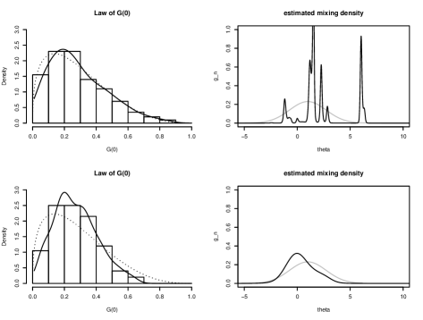
This behavior is illustrated in Figure 1. We consider a location mixture of Gaussian distributions $\text{N}(\theta_{i},\sigma^{2})$, with $\sigma^{2}$ known. In this case, the assumptions of Theorem 3.4 are satisfied, and $G$ is absolutely continuous, a.s. The prior guess $G_{0}$ is $\text{N}(1,3)$. The weights in Newton’s recursions are $\alpha_{n}=1/(\alpha+n)$, with $\alpha=5$. Were $G\sim\text{DP}(\alpha,G_{0})$, then, for any set $A$, the law of $G(A)$ would be a Beta distribution, with parameters $(\alpha G_{0}(A),\alpha(1-G_{0}(A))$. The panels in the first column of Figure 1 compare such Beta density (gray dotted line), for $A=(-\infty,0]$, with a Monte Carlo approximation of the law of $G(0)$ arising from the c.i.d. model. The Monte Carlo sample is obtained by generating samples $x_{1:N}^{(m)}$, $m=1,\ldots,200$ from the c.i.d. model (10), with $N=1000$. For each sample, we compute $G_{N}(0)$, that we take as a fairly reasonable proxy of the realization of the random $G(0)$. The first raw in Figure 1 corresponds to $\sigma^{2}=0.01$. In the second raw, $\sigma^{2}=1$. Clearly, the results do not contradict the conjecture that, if $\sigma^{2}$ is (very) small, the law of $G$ is close to the DP. The shrinkage effect that replaces the DP random partition of $\theta_{1:N}$ is illustrated in the right panels of Figure 1, which show the density estimate $g_{n}$ in the two cases. Clearly, for $\sigma^{2}=0.01$, $g_{n}$ closely describes a random partition of the $\theta_{n}$.

4 Asymptotic posterior laws

By part (ii) of Theorem 3.1, Newton’s rule $G_{n}$ can be regarded as a point estimate, with respect to quadratic loss, of the limit mixing distribution $G$, in a quasi-Bayes mixture model. Yet, a Bayesian mixture model would offer more than a point estimate; it would give a description of the uncertainty through the posterior distribution of $G\mid x_{1:n}$. The probabilistic framework we have provided for Newton’s learning rule allows to go beyond point estimation, studying the conditional distribution of $G$, given $x_{1:n}$. We first obtain an asymptotic Gaussian approximation of the conditional distribution of $G(A)$, given $x_{1:n}$, for any measurable set $A$. We then extend the results to the joint conditional distribution of a random vector $[G(A_{1}),\ldots,G(A_{k})]^{\prime}$, for any measurable $A_{1},\ldots A_{k}$.

4.1 Asymptotic posterior distribution and credible intervals.

Let us recall that $P$ is a probability law for $(X_{n})$, consistent with the assumptions (10). Here we give an asymptotic Gaussian approximation of the conditional law $P(G(A)\in\cdot\mid x_{1:n})$, for a measurable set $A$. The almost sure conditional convergence involved is a strong form of convergence (Crimaldi (2009)), that implies stable convergence (Renyi (1963), Aldous (1985), Häusler and Luschgy (2015)) and convergence in distribution of the unconditional law.

Notice that, although having a similar flavor, these results differ from Bernstein-von-Mises types of theorems, which are stated a.s. with respect to the law $P_{G_{true}}^{\infty}$. The law $P$ describes an evolutionary process and the results inform about the rate of convergence of $G_{n}(A)(x_{1:n})$ to the limit distribution $G(A)(x_{1},x_{2},\dots)$, for any $\omega=(x_{1},x_{2},\ldots)$ in a set of $P$-probability one. Berstein-von-Mises results are beyond the aims of this paper, but we will give some hints in the simulation study in Section 5.

Let us denote by $\text{N}(\mu,\sigma^{2})$ the Gaussian law with mean $\mu$ and variance $\sigma^{2}$, and by $\Phi(t\mid\mu,\sigma^{2})$ its d.f. evaluated at $t$. A $\text{N}(0,0)$ law is interpreted as the law degenerate at zero. The $p$-dimensional Gaussian law will be denoted by $\text{N}_{p}$, with d.f. $\Phi_{p}$. Without loss of generality, we can assume that $f_{G_{0}}(x)\neq 0$ for every $x\in\mathbb{X}$. This implies

$$f_{G_{n}}(x)\neq 0\quad\mbox{for every $x\in\mathbb{X}$ and $n\geq 0$}.$$ (18)

Our first result finds a sequence $(r_{n})$ such that the conditional distribution of $\sqrt{r_{n}}(G(A)-G_{n}(A))$, given $X_{1:n}$, is asymptotically a zero-mean Gaussian law, with variance

$$V_{A}=\int_{\{x:f_{G}(x)\neq 0\}}P_{G}(A\mid x)^{2}dF_{G}(x)-G(A)^{2}.$$ (19)

We remind the notation $P_{H}(A\mid x)=\int_{A}f(x\mid\theta)dH(\theta)/\int_{\Theta}f(x\mid\theta)dH(\theta)$, for any d.f. $H$ on $\Theta$.

Before stating the theorem, we give the following Lemma. Let us define, for any $A\in\mathcal{B}(\Theta)$ and $n\geq 1$,

$$V_{A,n}=\int_{\mathbb{X}}P_{G_{n}}(A\mid x)^{2}dF_{G_{n}}(x)-G_{n}(A)^{2}.$$ (20)

Notice that $V_{A,n}$ can be written as $V_{A,n}=E((P_{G_{n}}(A\mid X_{n+1})-G_{n}(A))^{2}\mid X_{1:n})$, expressing the prior-to-posterior variability, given $X_{1:n}$, when $G_{n}$ plays the role of the prior and $P_{G_{n}}(\cdot\mid x_{n+1})$ of the posterior.

Lemma 4.1

For any $A\in\mathcal{B}(\Theta)$, $V_{A,n}$ converges to $V_{A}$ a.s. as $n\rightarrow\infty$.

We can then give the main results of this section.

Theorem 4.1

Let $(\alpha_{n})$ satisfy $\sum_{n}\alpha_{n}=\infty$ and $\sum_{n}\alpha_{n}^{2}<\infty$ and let $(r_{n})$ be a monotone sequence of positive numbers such that $r_{n}\sim(\sum_{k>n}\alpha_{k}^{2})^{-1}$ as $n\rightarrow\infty$. If

$$\sqrt{r_{n}}\sup_{k\geq n}\alpha_{k}\rightarrow 0$$ (21)

and

$$\sum_{k\geq 1}r_{k}^{2}\alpha_{k+1}^{4}<\infty,$$ (22)

then, for every $A\in\mathcal{B}(\Theta)$,

$$P(\sqrt{r_{n}}(G(A)-G_{n}(A))\leq t\mid X_{1:n})\rightarrow\Phi(t\mid 0,{V_{A}}),$$ (23)

with ${V_{A}}$ as in (19). If $\alpha_{n}=(\alpha+n)^{-\beta}$ with $1/2<\beta\leq 1$ and $\alpha>0$, then (23) holds with $r_{n}=(2\beta-1)n^{2\beta-1}$.

Remark 4.1

Assumptions (21) and (22) hold for most choices of $(\alpha_{n})$ satisfying $\sum_{n}\alpha_{n}=\infty$ and $\sum_{n}\alpha_{n}^{2}<\infty$. In particular, if $(\alpha_{n})$ is definitively decreasing, then (21) is a consequence of (22). A sufficient condition for (22) is

$$\alpha_{n}=(nb_{n})^{-1}$$

for a sequence $b_{n}$ which is definitively non increasing. Indeed, in this case

$$\limsup_{n\rightarrow\infty}r_{n-1}\alpha_{n}=\limsup_{n\rightarrow\infty}\frac{(nb_{n})^{-1}}{\sum_{k\geq n}(kb_{k})^{-2}}\leq\limsup_{n\rightarrow\infty}\frac{(nb_{n})^{-1}}{b_{n}^{-2}\sum_{k\geq n}k^{-2}}\leq\limsup_{n\rightarrow\infty}b_{n}<\infty.$$

In turn, this implies that $r_{n}^{2}\alpha_{n+1}^{4}<(\sup_{k}b_{k})^{2}\alpha_{n+1}^{2}$, for $n$ large enough, and therefore (22).

Remark 4.2

If $V_{A}(\omega)=0$, then Theorem 4.1 gives convergence to a degenerate distribution on zero. From the definition of $V_{A}$, it is immediate to see that $V_{A}(\omega)=0$ if and only if $P_{G}(A\mid X)(\omega)=G(A)(\omega)$, which happens if and only if $G(A)(\omega)$ is zero or one.

In Theorem 4.1, the limit variance $V_{A}$ is unknown, depending on $G$. By Lemma 4.1, a convergent estimator is provided by $V_{A,n}$. Replacing the random $V_{A}$ with its consistent estimate, to get an asymptotic distribution that allows to compute asymptotic credible intervals for $G(A)$ (as done through Cramér-Slutzky Theorem in standard i.i.d. settings) is here delicate, given the kind of convergence we are studying. Yet, we can prove the following

Theorem 4.2

Let $A\in\mathcal{B}(\Theta)$. Then, with $(r_{n})$ defined as in Theorem 4.1 and under the same assumptions, for almost all $\omega=(x_{1},x_{2},\dots)$ such that $V_{A}(\omega)>0$,

$$P(\sqrt{r_{n}}\frac{G(A)-G_{n}(A)}{\sqrt{V_{A,n}}}\leq t\mid x_{1:n})\rightarrow\Phi(t\mid 0,1).$$ (24)

If $\alpha_{n}=(\alpha+n)^{-\beta}$ with $1/2<\beta\leq 1$ and $\alpha>0$, then (24) holds with $r_{n}=(2\beta-1)n^{2\beta-1}$.

Theorems 4.1 and 4.2 allow to obtain asymptotic credible intervals. For a fixed set $A$, Theorem 4.2 gives that, for almost all $\omega=(x_{1},x_{2},\ldots)$ such that $V_{A}(\omega)>0$,

$$P(G_{n}(A)-z_{1-\gamma/2}\sqrt{V_{A,n}/r_{n}}<G(A)<G_{n}(A)+z_{1-\gamma/2}\sqrt{V_{A,n}/r_{n}}\mid x_{1:n})\approx 1-\gamma,$$

where $z_{1-\gamma/2}$ is the $(1-\gamma/2)$-quantile of the standard Gaussian distribution. If $V_{A}(\omega)=0$, then Theorem 4.1 implies that the limit distribution is degenerate on zero, therefore, for any $\epsilon>0$

$$P(G_{n}(A)-z_{1-\gamma/2}\sqrt{\epsilon/r_{n}}<G(A)<G_{n}(A)+z_{1-\gamma/2}\sqrt{\epsilon/r_{n}}\mid x_{1:n})\geq 1-\gamma,$$

asymptotically. It follows that, for every $\epsilon>0$,

$$\left[G_{n}(A)-z_{1-\gamma/2}\sqrt{\frac{max(V_{A,n},\epsilon)}{r_{n}}};G_{n}(A)+z_{1-\gamma/2}\sqrt{\frac{max(V_{A,n},\epsilon)}{r_{n}}}\right]$$

is an asymptotic credible interval for $G(A)$, of level at least $1-\gamma$.

4.2 Asymptotic joint posterior distribution and credible regions.

We now study the joint behavior of $[G_{n}(A_{1})-G(A_{1}),\dots,G_{n}(A_{k})-G(A_{k})]^{\prime}$, for any fixed choice of $A_{1},\dots,A_{k}\in\mathcal{B}(\Theta)$. As in the previous section, we assume that $f_{G_{0}}(x)\neq 0$ for every $x\in\mathbb{X}$, which implies (18). For every $n\geq 1$, and $A_{i},A_{i^{\prime}}$, let

$\displaystyle C_{A_{i},A_{i^{\prime}},n}$ $\displaystyle=Cov\left(P(\theta_{n+1}\in A_{i}\mid X_{1:n+1}),P(\theta_{n+1}\in A_{i^{\prime}}\mid X_{1:n+1})\mid X_{1:n}\right)$
$\displaystyle=\int_{\mathbb{X}}P_{G_{n}}(A_{i}\mid x)P_{G_{n}}(A_{i^{\prime}}\mid x)dF_{G_{n}}(x)-G_{n}(A_{i})G_{n}(A_{i^{\prime}}).$

Furthermore, let

$$C_{A_{i},A_{i^{\prime}}}=\int_{\{x:f_{G}(x)\neq 0\}}P_{G}(A_{i}\mid x)P_{G}(A_{i^{\prime}}\mid x)dF_{G}(x)-G(A_{i})G(A_{i^{\prime}}).$$

Following the same line of reasoning as in Lemma 4.1, it can be proved that, as $n\rightarrow\infty$,

$${C_{A_{i},A_{i^{\prime}},n}}\rightarrow{C_{A_{i},A_{i^{\prime}}}}\quad a.s.$$

Thus, the conditional covariance matrix

$$C_{n}(A_{1},\dots,A_{k}):=\left[C_{A_{i},A_{i^{\prime}},n}\right]_{i,i^{\prime}}.$$

converges a.s. to

$$C(A_{1},\dots,A_{k}):=\left[C_{A_{i},A_{i^{\prime}}}\right]_{i,i^{\prime}}.$$ (25)

Then we can prove

Theorem 4.3

In model (10), let $(\alpha_{n})$ satisfy $\sum_{n}\alpha_{n}=\infty$ and $\sum_{n}\alpha_{n}^{2}<\infty$. Let $(r_{n})$ be a monotone sequence of positive numbers such that $r_{n}\sim(\sum_{j>n}\alpha_{j}^{2})^{-1}$ as $n\rightarrow\infty$. If (21) and (22) hold, then, for every $k\geq 1$ and every $A_{1},\dots,A_{k}\in\mathcal{B}(\Theta)$,

$$P(\sqrt{r_{n}}\begin{bmatrix}G(A_{1})-G_{n}(A_{1})\\ \vdots\\ G(A_{k})-G_{n}(A_{k})\end{bmatrix}\in\cdot\mid X_{1:n})\rightarrow\Phi_{k}(\cdot\mid{\bf 0},C(A_{1},\dots,A_{k})),\quad\mbox{for $n\rightarrow\infty$},$$ (26)

with $C(A_{1},\dots,A_{k})$ as in (25). If $\alpha_{n}=(\alpha+n)^{-\beta}$ with $1/2<\beta\leq 1$ and $\alpha>0$, then (26) holds with $r_{n}=(2\beta-1)n^{2\beta-1}$.

The following result is the analogous of Theorem 4.2 for the joint posterior distribution.

Theorem 4.4

Under the same assumptions as in Theorem 4.3, for every $k\geq 1$ and every $A_{1},\dots,A_{k}\in\mathcal{B}(\Theta)$,

$$P\left(\sqrt{r_{n}}\;C_{n}(A_{1},\dots,A_{k})^{-1/2}\begin{bmatrix}G(A_{1})-G_{n}(A_{1})\\ \dots\\ G(A_{k})-G_{n}(A_{k})\end{bmatrix}\in\cdot\mid x_{1:n}\right)\rightarrow\Phi_{k}(\cdot\mid{\bf 0},I)\quad\mbox{for $n\rightarrow\infty$},$$

for almost all $\omega=(x_{1},x_{2},\ldots)$ such that $\det(C(A_{1},\dots,A_{k})(\omega))\neq 0$.

Based on Theorems 4.3 and 4.4, we can give an asymptotic credible region for $[G(A_{1}),\dots,G(A_{k})]^{\prime}$.

Proposition 4.1

Let $\mathbf{G}_{n}(\mathbf{A})=[G_{n}(A_{1}),\dots,G_{n}(A_{k})]$ and let $\chi^{2}_{1-\gamma}$ denote the $(1-\gamma)$-quantile of the chi-square distribution with $k$ degrees of freedom. Then, for every $\epsilon>0$, the set

$$E_{n}^{(\epsilon)}=\left\{\mathbf{s}\in\mathbb{R}^{k}:(\mathbf{s}-\mathbf{G}_{n}(\mathbf{A}))^{T}(C_{n}(A_{1},\dots,A_{k})+\epsilon I)^{-1}(\mathbf{s}-\mathbf{G}_{n}(\mathbf{A}))\leq\frac{\chi^{2}_{1-\gamma}}{r_{n}}\right\}$$

satisfies

$$\liminf_{n}P([G(A_{1}),\dots,G(A_{k})]^{\prime}\in E_{n}^{(\epsilon)}\mid X_{1:n})\geq 1-\gamma\quad a.s.$$

5 Simulation study: tuning the weights $\alpha_{n}$

The lack of exchangeability of Newton et al.’s rule implies that the mixing density estimate depends on the ordering of the observations. Indeed, the authors propose to use an average of the estimates obtained over random permutations of the original sample; see also Tokdar et al. (2009). Our study of the probabilistic model underlying Newton’s learning rule allows us to give new hints about how one can attenuate the effect of the ordering on the estimates.

Figure 2 shows the recursive estimate $g_{n}$ of the mixing density, given by (4), for different permutations of the observations. In the first column, the data is a random sample $x_{1:1000}$, simulated from a location mixture of Gaussian distributions, with $\sigma^{2}=1$. The true mixing distribution used in the simulation is $0.3\text{N}(-1,2)+0.7\text{N}(3,1.5)$ (plotted in dark gray), describing two groups in the $\theta_{i}$. The initial distribution $G_{0}$ is $\text{N}(1,9)$, fairly diffuse (gray, dashed). In the second and third column, the data are two different permutations of $x_{1:1000}$.

Refer to caption
Figure 2: Newton’s recursive estimate of the mixing density (black). The data in the first column is a simulated random sample of size $1000$ from a location mixture of Gaussian distributions, with $\sigma^{2}=1$, and mixing distribution $0.3\text{N}(-1,2)+0.7\text{N}(3,1.5)$ (plotted in dark gray). In the second and third columns, the data are two permutations of the sample in column one. The initial distribution $G_{0}$ is $\text{N}(1,9)$ (gray, dashed). The dashed lightgray to gray lines are the density estimates $g_{n}$ with $n=1;n=300$ and $n=500$, respectively. In the first and second rows, the weights are $\alpha_{n}=1/(\alpha+n)$, with $\alpha=1$ and $\alpha=100$, respectively. In the third row, the weights are as in (27).
Refer to caption
Figure 3: Recursive estimate of the mixing distribution: marginal asymptotic $0.95$ credible intervals for $G(t_{j})$, for $t_{j}$ as evidenced in the plot. The black line is the true mixing distribution. The data and the weights $\alpha_{n}$ are as in panels $[2,1]$ and $[3.1]$ of Figure 2.

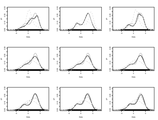
The black lines in the plots are the estimates $g_{n}$, for $n=1000$. The dashed light-gray to gray lines are the density estimates $g_{n}$ for $n=1;n=300$ and $n=500$, respectively. In the first row, the weights are $\alpha_{n}=1/(\alpha+n)$, with $\alpha=1$. The density estimates change sensitively for different permutations of the sample. We expect that a larger value of $\alpha$ may attenuate the sensitivity of the estimates to permutations, for the following reason. We have shown that Newton’s rule underlines an evolutionary, c.i.d. model, where the order (time, say) matters. Intuitively, the effect of the ordering is attenuated, if such evolution is milder. The example in Section 3 helps the intuition. The $\theta_{n}$ are not exchangeable, thus, there is no random latent distribution $G$ such that $\theta_{n}\mid G\overset{i.i.d}{\sim}G$. In the example, we envisage a sequence $(\tilde{G}_{n})$ of random distributions, that evolve over time from the initial distribution $G_{0}$. Such dynamics from $G_{0}$ is stronger, the larger is $\alpha_{n}$; thus, when $\alpha_{n}=1/(\alpha+n)$, the smaller is $\alpha$. This is evident by looking at (14): the variance of a DP increases, the smaller is the scale parameter. Thus, a large value of $\alpha$ not only expresses that $\tilde{G}_{1}\sim DP(\alpha G_{0})$ is concentrated around the (absolutely continuous) initial distribution $G_{0}$ (which is reasonable, as, in fact, Newton’s algorithm is thought for an absolutely continuous mixing distribution); but also, and we believe interestingly, it expresses a moderate evolution of $\tilde{G}_{n}$; thus, a situation closer to exchangeability. The second row of Figure 2 shows the density estimates $g_{n}$ with $\alpha_{n}=1/(\alpha+n)$ and $\alpha=100$. The data are the same as in the first row. The effect of the ordering of the observations is clearly attenuated.

However, these plots suggest that one is learning too slowly from the data. The weights $\alpha_{n}=1/(\alpha+n)$ decrease to zero too quickly. In fact, while, on one hand, one may want small weights $\alpha_{n}$ for $n$ small, to mitigate the evolution and the consequent sensitivity to permutations, on the other hand, the situation changes after a sufficiently large $n$. For $n$ large, the underlying random $\tilde{G}_{n}$ will be fairly close to its limit $G$, and one gets to a situation close to an exchangeable mixture model, with $\theta_{i}\mid G\overset{iid}{\approx}G$. Then, in order to learn from the data about $G$, the weights $\alpha_{n}$ should not be too small; that is, they should not converge to zero too quickly. The last row of Figure 2 shows the mixing density estimate $g_{n}$ obtained with weights

$$\alpha_{n}=\left\{\begin{array}[]{cc}1/(\alpha+n)&\mbox{ for}\;n\leq 500\\ 1/(\alpha+n)^{3/4}&\mbox{ for}\;n>500\end{array}\right.$$ (27)

with $\alpha=100$. This simple choice is yet very clear in demonstrating the above intuition. The effect of the ordering is attenuated, and the slower decrease to zero of the weights $\alpha_{n}$ improves learning. Roughly speaking, one uses the first part of the sample to induce some randomness around $G_{0}$; in other words, to learn about the prior distribution of $G$, in a sort of empirical Bayes fashion; then, after a sufficiently large $n$, the learning process proceeds as in an exchangeable mixture model, with the learned prior law.

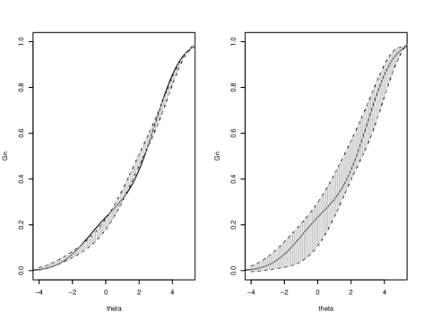
We finally consider inference on the mixing distribution function. A slower decay to zero of the $\alpha_{n}$ gives higher variability of $G_{n}$, which is reflected in higher conditional asymptotic variance of its limit $G$. We illustrate such effect in Figure 3. The plots show the $95\%$ asymptotic credible intervals for the random mixing distribution function $G$, given $x_{1:1000}$, for data and weights as in panels $[2,1]$ and $[3,1]$ of Figure 2. More precisely, we computed the marginal asymptotic credible intervals for $G(t_{j})$, for the $t_{j}$ as evidenced in the plots. The black line is the true mixing distribution used in the simulation. For $\alpha_{n}=1/(\alpha+n)$, with $\alpha=100$ (left panel), the interval is quite narrow. This is explained by the low variability of $G_{n}$, due to the fast decaying weights. With weights $\alpha_{n}$ as in (27), from Theorem 4.2 we obtain

$$G(t_{j})\mid x_{1:n}\approx\text{N}(G_{n}(t_{j}),\frac{V_{A,n}}{2\sqrt{n}}).$$

The larger credible intervals in the right panel of Figure 3 reflect the higher asymptotic conditional variance obtained in this case.

6 Proofs

This section provides the proofs of the previous results.

Proof of Theorem 3.1.

(i) For every $A\in\mathcal{B}(\Theta)$ and every $n\geq 0$,

$$E(G_{n+1}(A)\mid X_{1:n})=(1-\alpha_{n+1})G_{n}(A)+\alpha_{n+1}E(P(\theta_{n+1}\in A\mid X_{1:n+1})\mid X_{1:n})=G_{n}(A)$$ (28)

Hence, the sequence $(G_{n})$ is a measure valued martingale with respect to the natural filtration of $(X_{n})$. By Lemma 7.14 in Aldous (1985), there exists a random probability measure $G$ such that $G_{n}$ converges a.s. to $G$, in the topology of weak convergence.

(ii) Since, for every $A$, $(G_{n}(A))$ is uniformly bounded, it is a closed martingale. Thus, for every $n\geq 0$ and $k\geq 1$,

$$P(\theta_{n+k}\in A\mid X_{1:n})=E(P(\theta_{n+k}\in A\mid X_{1:n+k-1})\mid X_{1:n})=E(G_{n+k-1}(A)\mid X_{1:n})=E(G(A)\mid X_{1:n}).$$

$\square$

Proof of Proposition 3.1.

Let us denote by ${\cal F}_{n}$ the sigma field generated by $X_{1:n}$, and let ${\cal F}_{\infty}=\vee_{n}{\cal F}_{n}$ and $Z$ be a random variable such that $Z\mid{\cal F}_{\infty}\sim G$. We have

$\displaystyle E\left(\int_{\Theta}h(z)dG(z)\left|{\cal F}_{n}\right.\right)$ $\displaystyle=$ $\displaystyle E\left(E(h(Z)\mid{\cal F}_{\infty})\mid{\cal F}_{n}\right)=E(h(Z)\mid{\cal F}_{n})$
$\displaystyle=$ $\displaystyle\int_{\Theta}h(z)P(Z\in dz\mid{\cal F}_{n}),$

where the last equality follows from the fundamental property of regular conditional distributions (see e.g. Aldous (1985), eq.(2.4)). Noticing that $P(Z\in\cdot\mid{\cal F}_{n})=E(P(Z\in\cdot\mid{\cal F}_{\infty})\mid{\cal F}_{n})=E(G(\cdot)\mid{\cal F}_{n})$, we obtain

$$\int_{\Theta}h(\theta)dG_{n}(\theta)=E\left(\int_{\Theta}h(\theta)dG(\theta)\mid\mathcal{F}_{n}\right).$$ (29)

Since

$$E\left(\int_{\Theta}h(\theta)dG(\theta)\mid\mathcal{F}_{n}\right)\rightarrow E\left(\int_{\Theta}h(\theta)dG(\theta)\mid\mathcal{F}_{\infty}\right)\quad a.s.$$

and since $G$ is ${\cal F}$-measurable, then $\int_{\Theta}h(\theta)dG_{n}(\theta)\rightarrow\int_{\Theta}h(\theta)dG(\theta)$ a.s.

To prove the last assertion, notice that, from (29), $\int_{\Theta}|h(\theta)|dG_{0}(\theta)=E(\int_{\Theta}|h(\theta)|dG(\theta))$. Thus, if $\int_{\Theta}|h(\theta)|dG_{0}(\theta)<\infty$, then the non-negative quantity $\int_{\Theta}|h(\theta)|dG(\theta)$ is a.s. finite.
$\square$

Proof of Theorem 3.2

(i) To prove that $(X_{n})$ is c.i.d., it is enough to show that $P(X_{n+2}\in B\mid X_{1:n})=P(X_{n+1}\in B\mid X_{1:n})$, for any $n\geq 0$ and any $B$. This is an immediate consequence of the conditional independence of the $X_{i}$, given $(\theta_{n})$, and of Theorem 3.1. Indeed, denoting by $F(\cdot\mid\theta)$ the distribution corresponding to the density $f(\cdot\mid\theta)$, we have

$\displaystyle P(X_{n+2}\in B\mid X_{1:n})$ $\displaystyle=$ $\displaystyle E(P(X_{n+2}\in B\mid\theta_{n+2},X_{1:n})\mid X_{1:n})=\int_{\Theta}F(B\mid\theta)P(\theta_{n+2}\in d\theta\mid X_{1:n})$
$\displaystyle=$ $\displaystyle\int_{\Theta}F(B\mid\theta)P(\theta_{n+1}\in d\theta\mid X_{1:n})=P(X_{n+1}\in B\mid X_{1:n}),$

where the third equality follows from (28).

(ii) Let $(t_{j},j\in J)$ be a countable dense set of points in $\mathbb{X}$. By Proposition 3.1, $F_{G_{n}}(t_{j})\rightarrow F_{G}(t_{j})$, for every $\omega\in\Omega_{j}$ with $P(\Omega_{j})=1$. Now, let $\Omega^{*}=\cap_{j}\Omega_{j}$. Being $J$ countable, $P(\Omega^{*})=1$, and for any $\omega\in\Omega^{*}$, $F_{G_{n}}(t_{j})\rightarrow F_{G}(t_{j})$ for all $t_{j}$. For distribution functions, convergence on a countable dense set implies weak convergence. Therefore, we have that, $P$-a.s., $F_{G_{n}}$ converges to $F_{G}$ in the topology of weak convergence. Now, notice that $F_{G}$ is a.s. absolutely continuous, with density $f_{G}$. By Theorem 1 in Berti et al. (2013), a.s. weak convergence of the predictive measures to an absolutely continuous random measure implies that the convergence also holds in total variation. Therefore, $P$-a.s., $F_{G_{n}}$ converges to $F_{G}$ in total variation, which is equivalent to $f_{G_{n}}{\overset{L_{1}}{\rightarrow}}f_{G}$.

(iii) Convergence of the predictive distributions to the random probability measure $F_{G}$ implies that $(X_{n})$ is asymptotically exchangeable, with directing measure $F_{G}$ (Aldous (1985), Lemma 8.2).
$\square$

Proof of Theorem 3.3

Let $\mathcal{H}$ be a a countable, convergence determining class of bounded continuous functions, and $k$ a positive integer. By Theorem 3.2, $(X_{n})$ is asymptotically exchangeable with directing random measure $F_{G}$; therefore, for almost all $\omega=(x_{1},x_{2},\dots)$

$$E(\prod_{i=1}^{k}h_{i}(X_{n+i})\mid x_{1:n})\rightarrow\prod_{i=1}^{k}\left(\int_{\Theta}\int_{\mathbb{X}}h_{i}(z_{i})f(z_{i}\mid s_{i})d\mu(z_{i})dG(s_{i})(\omega)\right),$$ (30)

for every $h_{i}\in\mathcal{H}$. Let $\omega=(x_{1},x_{2},\dots)$ be fixed in such a way that the above equations hold. Then, for every $j=1,\dots,k$, the sequence of probability measures $\left(P(\theta_{n+j}\in\cdot\mid x_{1:n})\right)$ is tight. It follows that the sequence of joint conditional distributions $\left(P(\theta_{n+1:n+k}\in\cdot\mid x_{1:n})\right)$ is tight. Thus, for every increasing sequence of integers, there exists a subsequence $(n_{j})$ and a probability measure $Q(\omega)$ such that $P((\theta_{n_{j}+1},\dots,\theta_{n_{j}+k})\in\cdot\mid x_{1:n_{j}})\rightarrow Q(\omega)$. The proof is complete if we can show that

$$Q(A_{1}\times\dots\times A_{k})(\omega)=\prod_{i=1}^{k}G(A_{i})(\omega),\quad\mbox{for every $A_{1},\dots A_{k}$},$$ (31)

because (31) implies that the conditional law of $(\theta_{n_{j}+1},\dots,\theta_{n_{j}+k})$ converges weakly to the product measure $G^{k}$. The sequence of random variables $\left(\prod_{i=1}^{k}\int_{\mathbb{X}}h_{i}(z_{i})f(z_{i}\mid\theta_{n+i})d\mu(z_{i})\right)$ is uniformly bounded and, therefore, it is uniformly integrable. Hence,

$\displaystyle\int_{\Theta^{k}}\prod_{i=1}^{k}\int_{\mathbb{X}}h_{i}(z_{i})f(z_{i}\mid s_{i})d\mu(z_{i})$ $\displaystyle P((\theta_{n_{j}+1},\dots\theta_{n_{j}+k})\in(ds_{1},\dots,ds_{k})\mid x_{1:n_{j}})$
$\displaystyle\rightarrow\int_{\Theta^{k}}\prod_{i=1}^{k}\int_{\mathbb{X}}h_{i}(z_{i})f(z_{i}\mid s_{i})d\mu(z_{i})dQ(s_{1},\dots,s_{k})(\omega),$

for every $h_{1},\dots,h_{k}\in\mathcal{H}$. On the other hand, by (30),

$\displaystyle\int_{\Theta^{k}}\prod_{i=1}^{k}\int_{\mathbb{X}}h_{i}(z_{i})f(z_{i}\mid s_{i})d\mu(z_{i})$ $\displaystyle P((\theta_{n_{j}+1},\dots\theta_{n_{j}+k})\in(ds_{1},\dots,ds_{k})\mid x_{1:n_{j}})$
$\displaystyle\rightarrow\int_{\Theta^{k}}\prod_{i=1}^{k}\int_{\mathbb{X}}h_{i}(z_{i})f(z_{i}\mid s_{i})d\mu(z_{i})dG(s_{1})(\omega)\dots dG(s_{k})(\omega).$

Hence, for every $h_{1},\dots,h_{k}\in\mathcal{H}$,

$\displaystyle\int_{\Theta^{k}}\prod_{i=1}^{k}\int_{\mathbb{X}}h_{i}(z_{i})f(z_{i}\mid s_{i})$ $\displaystyle d\mu(z_{i})dQ(s_{1},\dots,s_{k})(\omega)$ (32)
$\displaystyle=\int_{\Theta^{k}}\prod_{i=1}^{k}\int_{\mathbb{X}}h_{i}(z_{i})f(z_{i}\mid s_{i})d\mu(z_{i})dG(s_{1})(\omega)\dots dG(s_{k})(\omega).$

Since the model is identifiable, the class

$$\left\{\int h(z)f(z\mid\theta)d\mu(z):h\in\mathcal{H}\right\}$$

is separating for $\mathcal{P}(\Theta)$. It follows that the class

$$\left\{\prod_{i=1}^{k}\int h_{i}(z)f(z\mid\theta)d\mu(z):h_{i}\in\mathcal{H},i=1,\dots,k\right\}$$

is separating for $\mathcal{P}(\Theta^{k})$ (Ethier and Kurtz (1986), Proposition 3.4.6). Thus, (32) implies (31).
$\square$


Proof of Theorem 3.4. The thesis follows from Lemmas 3.1 and 3.2, if we can show that

$$\sup_{n}E\left(\int_{K}g_{n}(\theta)^{2}d\lambda(\theta)\right)<\infty\quad\mbox{ for every }K\mbox{ compact, satisfying }\lambda(K)<\infty.$$ (33)

Let $K$ be a fixed compact set, with $\lambda(K)<\infty$. It holds

$$E\left(\int_{K}g_{n}(\theta)^{2}d\lambda(\theta)\right)=\int_{K}E(g_{n}(\theta)^{2})d\lambda(\theta)=\int_{K}E(E(g_{n}(\theta)^{2}\mid X_{1:n-1}))d\lambda(\theta).$$

By the martingale property of the sequence $(g_{n})$, and Jensen inequality, we obtain

$\displaystyle E\left(g_{n}(\theta)^{2}\mid X_{1:n-1}\right)$ $\displaystyle=g_{n-1}(\theta)^{2}E\left(\left[1+\alpha_{n}\left(\frac{f(X_{n}\mid\theta)}{\int_{\Theta}f(X_{n}\mid\theta^{\prime})g_{n-1}(\theta^{\prime})d\lambda(\theta^{\prime})}-1\right)\right]^{2}\mid X_{1:n-1}\right)$
$\displaystyle\leq g_{n-1}(\theta)^{2}\left[1+\alpha_{n}^{2}\left(1+\int_{\mathbb{X}}\frac{f(x\mid\theta)^{2}}{\int_{K}f(x\mid\theta^{\prime})g_{n-1}(\theta^{\prime})d\lambda(\theta^{\prime})}d\mu(x)\right)\right]$
$\displaystyle\leq g_{n-1}(\theta)^{2}\left[1+\alpha_{n}^{2}\left(1+\int_{\mathbb{X}}\int_{K}\frac{f(x\mid\theta)^{2}}{f(x\mid\theta^{\prime})}g_{n-1}(\theta^{\prime})d\lambda(\theta^{\prime})d\mu(x)\right)\right]$
$\displaystyle\leq g_{n-1}(\theta)^{2}\left[1+\alpha_{n}^{2}\left(1+\sup_{\theta_{1},\theta_{2}\in K}\int_{\mathbb{X}}\frac{f(x\mid\theta_{1})^{2}}{f(x\mid\theta_{2})}d\mu(x)\right)\right].$

Therefore

$$E\left(\int_{K}g_{n}(\theta)^{2}d\lambda(\theta)\right)\leq E\left(\int_{K}g_{n-1}(\theta,)^{2}d\lambda(\theta)\right)\left[1+\alpha_{n}^{2}\left(1+\sup_{\theta_{1},\theta_{2}\in K}\int_{\mathbb{X}}\frac{f(x\mid\theta_{1})^{2}}{f(x\mid\theta_{2})}d\mu(x)\right)\right]$$

Iterating, we obtain

$$E\left(\int_{K}g_{n}(\theta)^{2}d\lambda(\theta)\right)\leq\int_{K}g_{0}(\theta)^{2}d\lambda(\theta)\prod_{i=1}^{n}\left(1+\alpha_{i}^{2}M_{K}\right)$$

with $M_{K}=\left(1+\sup_{\theta_{1},\theta_{2}\in K}\int_{\mathbb{X}}\frac{f(x\mid\theta_{1})^{2}}{f(x\mid\theta_{2})}d\mu(x)\right)$, which is finite by the assumption (17). By (16), $\sup_{n}E(\int_{K}g_{n}(\theta)^{2}d\lambda(\theta))<\infty$.
$\square$

Proof of Lemma 4.1.

Since $G_{n}(A)\rightarrow G(A)$ a.s., it remains to show that

$$\int_{\mathbb{X}}P_{G_{n}}(A\mid x)^{2}dF_{G_{n}}(x)\rightarrow\int_{\{x:f_{G}(x)\neq 0\}}P_{G}(A\mid x)^{2}dF_{G}(x)\quad a.s.$$

By Theorem 3.2, $F_{G_{n}}$ converges to $F_{G}$ in total variation, a.s.; therefore

$$\int_{\{x:f_{G}(x)=0\}}P_{G_{n}}(A\mid x)^{2}dF_{G_{n}}(x)\leq F_{G_{n}}(\{x:f_{G}(x)=0\})\rightarrow F_{G}(\{x:f_{G}(x)=0\})=0\quad a.s.$$

Then, denoting $\mathbb{X}_{0}=\{x:f_{G}(x)\neq 0\}$, we have

$\displaystyle\left|\int_{\mathbb{X}_{0}}P_{G_{n}}(A\mid x)^{2}dF_{G_{n}}(x)-\int_{\mathbb{X}_{0}}P_{G}(A\mid x)^{2}dF_{G}(x)\right|$
$\displaystyle\leq$ $\displaystyle\int_{\mathbb{X}_{0}}|f_{G_{n}}(x)-f_{G}(x)|d\mu(x)+\left|\int_{\mathbb{X}_{0}}P_{G_{n}}(A\mid x)^{2}(x)dF_{G}(x)-\int_{\mathbb{X}_{0}}P_{G}(A\mid x)^{2}dF_{G}(x)\right|$

The first term converges to zero since $f_{G_{n}}$ converges to $f_{G}$ in $L_{1}$, by Theorem 3.2; the second term converges to zero by dominated convergence theorem. Thus, the thesis follows.
$\square$

Proof of Theorem 4.1.

For every $n\geq 1$, let

$$M_{n,j}=\left\{\begin{array}[]{ll}\sqrt{r_{n}}(G_{n}(A)-G_{n+j-1}(A))&j\geq 1\\ 0&j=0\end{array}\right.$$

and let

$$\mathcal{F}_{n,j}=\left\{\begin{array}[]{ll}\mathcal{F}_{n+j-1}&j\geq 1\\ \mathcal{F}_{n}&j=0,\end{array}\right.$$

where $({\cal F}_{n})$ is the natural filtration of $(X_{n})$. For every $n\geq 1$, $(M_{n,j})_{j\geq 0}$ is a zero-mean martingale, with respect to the filtration $(\mathcal{F}_{n,j})_{j\geq 0}$ and $\mathcal{F}_{n,1}=\mathcal{F}_{n}\subset\mathcal{F}_{n+1}=\mathcal{F}_{n+1,1}$. Let

$$Z_{n,j}:=M_{n,j}-M_{n,j-1}\mbox{ for }j\geq 1,\quad U_{n}:=\sum_{j\geq 1}Z_{n,j}^{2},\quad Z_{n}^{*}:=\sup_{j\geq 1}|Z_{n,j}|.$$

The thesis follows from Theorem A.1 in Crimaldi (2009) if we can show that $(Z_{n}^{*})$ is dominated in $L^{1}$ and that $(U_{n})$ converges a.s. to $V_{A}$.

By definition, $Z_{n,1}=0$ and, for $j\geq 2$,

$\displaystyle Z_{n,j}$ $\displaystyle=\sqrt{r_{n}}\left(G_{n+j-2}(A)-G_{n+j-1}(A)\right)$
$\displaystyle=\sqrt{r_{n}}\alpha_{n+j-1}\left(G_{n+j-2}(A)-\frac{\int_{A}f(X_{n+j-1}\mid\theta)dG_{n+j-2}(\theta)}{\int_{\Theta}f(X_{n+j-1}\mid\theta)dG_{n+j-2}(\theta)}\right).$

Since $\sqrt{r_{n}}\sup_{k\geq n}\alpha_{k}\rightarrow 0$, then $(Z_{n}^{*})$ is dominated in $L^{1}$.
To prove that $(U_{n})$ converges a.s. to $V_{A}$, we employ Lemma A.1 in Crimaldi et al. (2016). To be consistent with the notation therein, let us set $b_{1}=r_{1}$ and, for $k\geq 1$,

$$b_{k+1}=r_{k}\quad\mbox{ and }\quad a_{k}=\frac{1}{b_{k}^{2}\alpha_{k}^{2}}.$$

Then, we can write

$\displaystyle U_{n}$ $\displaystyle=b_{n+1}\sum_{j\geq 2}\alpha_{n+j-1}^{2}\left(\frac{\int_{A}f(X_{n+j-1}\mid\theta)dG_{n+j-2}(\theta)}{\int_{\Theta}f(X_{n+j-1}\mid\theta)dG_{n+j-2}(\theta)}-G_{n+j-2}(A)\right)^{2}$
$\displaystyle=b_{n+1}\sum_{k\geq n+1}\frac{Y_{k}}{a_{k}b_{k}^{2}},$

where

$$Y_{k}=\left(\frac{\int_{A}f(X_{k}\mid\theta)dG_{k-1}(\theta)}{\int_{\Theta}f(X_{k}\mid\theta)dG_{k-1}(\theta)}-G_{k-1}(A)\right)^{2}.$$

It can be proved, proceeding as in Lemma 4.1, that

$$E(Y_{k}\mid\mathcal{F}_{k-1})=E\left(\left[\frac{\int_{A}f(X_{k}\mid\theta)dG_{k-1}(\theta)}{\int_{\Theta}f(X_{k}\mid\theta)dG_{k-1}(\theta)}-G_{k-1}(A)\right]^{2}\mid\mathcal{F}_{k-1}\right)\rightarrow V_{A}\quad a.s.$$

as $k\rightarrow\infty$. Moreover,

$$\sum_{k\geq 1}\frac{E(Y_{k}^{2})}{a_{k}^{2}b_{k}^{2}}<\infty,$$

as $\sum_{k\geq 1}(a_{k}b_{k})^{-2}=\sum_{k\geq 1}\alpha_{k}^{4}b_{k}^{2}<\infty$ and $|Y_{k}|\leq 1$. Since, by assumption, $b_{n+1}\sum_{k\geq n+1}(a_{k}b_{k}^{2})^{-1}=r_{n}\sum_{k>n}\alpha_{k}^{2}\rightarrow 1,$ then, by Lemma A.1 in Crimaldi et al. (2016), $U_{n}\rightarrow V_{A}$ a.s. as $n\rightarrow\infty$.
$\square$

Proof of Theorem 4.2.

We first prove that, for every $A\in\mathcal{B}(\Theta)$, the conditional distribution of $(\sqrt{r_{n}}(G_{n}(A)-G(A)),{V_{A,n}})$, given $X_{1:n}$, converges to $\text{N}(0,{V_{A}})\times\delta_{V_{A}}$ a.s. on the set $\{\omega:V_{A}(\omega)>0\}$, $\omega=(x_{1},x_{2},\ldots)$. To show this, we use Lemma 4.1 and compute the joint characteristic function

$\displaystyle E(\exp(\mathrm{i}s_{1}\sqrt{r_{n}}(G(A)-G_{n}(A))+\mathrm{i}s_{2}{V_{A,n}})\mid X_{1:n})$ $\displaystyle=E(\exp(\mathrm{i}s_{1}\sqrt{r_{n}}(G(A)-G_{n}(A)))\mid X_{1:n})\exp(\mathrm{i}s_{2}{V_{A,n}})$
$\displaystyle\rightarrow\exp(-s_{1}^{2}{V_{A}}/2)\exp(\mathrm{i}s_{2}{V_{A}})$

Let now $\mathcal{D}$ be a countable convergence-determining class of bounded continuous functions for the probability measures on $\mathbb{R}$ and let

$$D_{n}=\sqrt{r_{n}}(G(A)-G_{n}(A)),\quad W_{n}=\frac{1}{\sqrt{V_{A,n}}}1_{(V_{A,n}>0)},\quad W=\frac{1}{\sqrt{V_{A}}}1_{(V_{A}>0)}.$$

Then $W_{n}(\omega)\rightarrow W(\omega)$ for almost all $\omega$ such that $V_{A}(\omega)>0$. By Theorem 4.1, for every $h\in\mathcal{D}$,

$$E(h(D_{n})\mid X_{1:n})1_{(V_{A}>0)}\rightarrow\int h(x)\phi(x\mid 0,1/W^{2})dx\quad a.s.$$

where $\phi(x\mid\mu,\sigma^{2})$ denotes the $\text{N}(\mu,\sigma^{2})$ density computed at $x$. Since $W_{n}$ is a function of $X_{1:n}$, then for every $h_{1},h_{2}\in\mathcal{D}$,

$\displaystyle E(h_{1}(D_{n})h_{2}(W_{n})\mid X_{1:n})1_{(V_{A}>0)}$ $\displaystyle=E(h_{1}(D_{n})\mid X_{1:n})h_{2}(W_{n})1_{(V_{A}>0)}$
$\displaystyle\rightarrow\int h_{1}(x)\phi(x\mid 0,1/W^{2})dxh_{2}(W)1_{(V_{A}>0)}$
$\displaystyle=\int h_{1}(x_{1})h_{2}(x_{2})d(\text{N}(0,1/W^{2})\times\delta_{W})(x_{1},x_{2})\,1_{(V_{A}>0)}$

Being the class $\{h_{1}h_{2}:h_{1},h_{2}\in\mathcal{D}\}$ a convergence determining class for the probability measures on ${\mathbb{R}}^{2}$, then, for every bounded continuous function $h$,

$\displaystyle E\left(h\left(\sqrt{r_{n}}\frac{G(A)-G_{n}(A)}{\sqrt{V_{A,n}}}\right)\mid X_{1:n}\right)=E(h(D_{n}W_{n})\mid X_{1:n})$
$\displaystyle\rightarrow\int h(xW)\phi(x\mid 0,1/W^{2})dx=\int h(y)\phi(y\mid 0,1)dy.$

a.s. on the set $\{\omega:V_{A}(\omega)>0\}$. $\square$

Proof of Theorem 4.3

Let $c_{1},\dots,c_{k}$ be arbitrary real numbers. The sequence $(\sum_{i=1}^{k}c_{i}G_{n}(A_{i}))_{n\geq 1},$ is a bounded martingale, converging a.s. to $\sum_{i=1}^{k}c_{i}G(A_{i})$. Following the same steps as in Theorem 4.1, with $\sum_{i=1}^{k}c_{i}G_{n}(A_{i})$ in the place of $G_{n}(A)$ and $\sum_{i=1}^{k}c_{i}G(A_{i})$ in the place of $G(A)$, we obtain

$$P(\sqrt{r_{n}}(\sum_{i=1}^{k}c_{i}G(A_{i})-\sum_{i=1}^{k}c_{i}G_{n}(A_{i}))\leq t\mid x_{1:n})\rightarrow\Phi(t;0,U),\quad\mbox{for any $t$},$$

where $U$ is the a.s. limit of

$$U_{n}:=r_{n}\sum_{j\geq n+1}\alpha_{j}^{2}Y_{j}$$

with

$\displaystyle Y_{j}$ $\displaystyle=\left[\sum_{i=1}^{k}c_{i}\left(P(\theta_{j}\in A_{i}\mid X_{1:j})-P(\theta_{j}\in A_{i}\mid X_{1:j-1})\right)\right]^{2}.$

Applying Lemma A.1 in Crimaldi et al. (2016), as in the proof of Theorem 4.1, and noticing that

$\displaystyle E(Y_{j}\mid X_{1:j-1})$ $\displaystyle=\sum_{i,i^{\prime}}c_{i}c_{i^{\prime}}\left[\int_{\mathbb{X}}P_{G_{j-1}}(A_{i}\mid x)P_{G_{j-1}}(A_{i^{\prime}}\mid x)dF_{G_{j-1}}(x)-G_{j-1}(A_{i})G_{j-1}(A_{i^{\prime}})\right]$
$\displaystyle\rightarrow\sum_{i,i^{\prime}}c_{i}c_{i^{\prime}}\left[\int_{\mathbb{X}}P_{G}(A_{i}\mid x)P_{G}(A_{i^{\prime}}\mid x)dF_{G}(x)-G(A_{i})G(A_{i^{\prime}})\right]$
$\displaystyle=\sum_{i,i^{\prime}=1}^{j}c_{i}c_{i^{\prime}}C_{A_{i},A_{i^{\prime}}},$

we obtain $U=\sum_{i,i^{\prime}=1}^{k}c_{i}c_{i^{\prime}}C_{A_{i},A_{i^{\prime}}}$. Thus, for every $c_{1},\dots,c_{k}$,

$$P(\sqrt{r_{n}}(\sum_{i=1}^{k}c_{i}G(A_{i})-\sum_{i=1}^{k}c_{i}G_{n}(A_{i}))\leq t\mid X_{1:n})\rightarrow\Phi(t\mid 0,\sum_{i,i^{\prime}=1}^{k}c_{i}c_{i^{\prime}}C_{A_{i},A_{i^{\prime}}}),\quad\mbox{a.s.}$$

for every $t$. The thesis follows from Cramér-Wold theorem.
$\square$

Proof of Theorem 4.4.

Let $({\cal F}_{n})$ denote the natural filtration of $(X_{n})$. Consider the ${\cal F}_{n}$-measurable spectral decomposition

$$\frac{C_{n}(A_{1},\dots,A_{k})}{r_{n}}=Q_{n}\Lambda_{n}Q_{n}^{T}$$

where $Q_{n}$ in a $k\times k$ orthogonal matrix and $\Lambda_{n}=diag(\lambda_{1}^{(n)},\dots,\lambda_{k}^{(n)})$. Let

$$Y^{(n)}=Q_{n}^{T}\left[\begin{array}[]{c}G(A_{1})-G_{n}(A_{1})\\ \dots\\ G(A_{k})-G_{n}(A_{k})\end{array}\right]$$

and

$$Z_{i}^{(n)}=\frac{Y_{i}^{(n)}}{\sqrt{\lambda_{i}^{(n)}}}1_{(\lambda_{i}^{(n)}\neq 0)}+\tilde{Z}_{i}1_{(\lambda_{i}^{(n)}=0)},$$

where $\tilde{Z}_{1}^{(n)},\dots,\tilde{Z}_{k}^{(n)}$ are i.i.d. random variables, independent of $\mathcal{F}_{n}$, and with $\text{N}(0,1)$ distribution. Then

$$\left[\begin{array}[]{c}G(A_{1})-G_{n}(A_{1})\\ \dots\\ G(A_{k})-G_{n}(A_{k})\end{array}\right]=Q_{n}\Lambda_{n}^{1/2}Z^{(n)}=\frac{C_{n}(A_{1},\dots,A_{j})^{1/2}}{\sqrt{r}_{n}}Z_{*}^{(n)}$$

where $Z_{*}^{(n)}=Q_{n}Z^{(n)}\approx\text{N}(0,I)$, given $\mathcal{F}_{n}$.

$\square$

Proof of Proposition 4.1 .

With the same notation as in the proof of Theorem 4.3, we can write

$\displaystyle\liminf_{n}P((G(A_{1}),\dots,G(A_{k})\in E_{n}^{(\epsilon)}\mid\mathcal{F}_{n})$
$\displaystyle\geq\liminf_{n}P\left(Z_{*}^{(n)T}\frac{C_{n}(A_{1},\dots,A_{k})^{1/2}}{\sqrt{r_{n}}}\left(\frac{C_{n}(A_{1},\dots,A_{k})+\epsilon I}{r_{n}}\right)^{-1}\frac{C_{n}(A_{1},\dots,A_{k})^{1/2}}{\sqrt{r_{n}}}Z_{*}^{(n)}\leq\chi^{2}_{1-\gamma}\mid\mathcal{F}_{n}\right)$
$\displaystyle\geq\liminf_{n}P(Z_{*}^{(n)T}Z_{*}^{(n)}\leq\chi^{2}_{1-\gamma}\mid\mathcal{F}_{n})=1-\gamma.$

$\square$

7 Discussion

For its simplicity and good practical performance, Newton’s algorithm is widely used in problems involving hidden variables. We have proposed a novel approach to study its properties, and make users more aware of the modeling assumptions implicitly made. We believe that our approach can be useful in other settings, too. Further explicit results on the probability law of the limit mixing distribution $G$, although difficult, could lead to novel priors for Bayesian nonparametrics on the space of absolutely continuous distributions. Modifications of the algorithm could be envisaged (as suggested in the simulation study of Section 5, or by initializing the procedure with exact computations from the DP mixture model) to control the prior distribution on $G$.

A limitation of Newton’s algorithm is that it requires to evaluate an integral at each step. An interesting class of recursive algorithms, that allow to overcome this difficulty, has been recently proposed by Hahn et al. (2018). Multivariate extensions are in Cappello and Walker (2018). Directions of research are extensions of our study to this class of algorithms, as well as developments for multivariate mixtures and dependent mixture models, possibly exploiting theoretical results on partially c.i.d. sequences (Fortini et al. (2017)).


Acknowledgments This work benefited from discussions with Lorenzo Cappello and Stephen Walker, to whom we express our thanks. The authors acknowledge financial support by the PRIN grant 2015SNS29B.

References

  • Airoldi et al. [2014] E.M. Airoldi, T. Costa, F. Bassetti, F. Leisen, and M. Guindani. Generalized species sampling priors with latent Beta reinforcements. J. Am. Stat. Assoc., 109:1466–1480, 2014.
  • Aldous [1985] D.J. Aldous. Exchangeability and related topics. École d’Été de Probabilités de Saint-Flour XIII 1983, 1117:1–198, 1985.
  • Bassetti et al. [2010] F. Bassetti, I. Crimaldi, and F. Leisen. Conditionally identically distributed species sampling sequences. Adv. Appl. Probab., 42:433–459, 2010.
  • Berti et al. [2004] P. Berti, L. Pratelli, and P. Rigo. Limit theorems for a class of identically distributed random variables. Ann. Probab., 32:2029–2052, 2004.
  • Berti et al. [2013] P. Berti, L. Pratelli, and P. Rigo. Exchangeable sequences driven by absolutely continuoous random measures. Ann. Probab., 41:2090–2102, 2013.
  • Broderick et al. [2013] T. Broderick, N. Boyd, A. Wibisono, A. C. Wilson, and M.I. Jordan. Streaming variational Bayes. In Proceedings of the 26th International Conference on Neural Information Processing Systems - Volume 2, pages 1727–1735. Curran Associates Inc., USA, 2013.
  • Cappello and Walker [2018] L. Cappello and S.G. Walker. A Bayesian motivated Laplace inversion for multivariate probability distributions. Methodol. Comp. Appl., 20:777–797, 2018.
  • Christian A. Naesseth et al. [2018] C.A. Christian A. Naesseth, S.W. Linderman, R. Ranganath, and D.M. Blei. Variational sequential Monte Carlo. In Proceedings of the 21st International Conference on Artificial Intelligence and Statistics, 2018.
  • Crimaldi [2009] I. Crimaldi. An almost sure conditional convergence result and an application to a generalized Pólya urn. Int. Math. Forum, 23:1139–1156, 2009.
  • Crimaldi et al. [2016] I. Crimaldi, P. Dai Pra, and I.G. Minelli. Fluctuation theorems for synchronization of interacting Pólya’s urns. Stochastic Process. Appl., 126:930–947, 2016.
  • Ethier and Kurtz [1986] S.N. Ethier and T.G. Kurtz. Markov Processes: Characterization and Convergence. New York:Wiley, Second edition, 1986.
  • Fortini et al. [2017] S. Fortini, S. Petrone, and P. Sporysheva. On a notion of partially conditionally identically distributed sequences. Stoch. Process. Their Appl., 128:819–846, 2017.
  • Ghosh and Tokdar [2006] J.K. Ghosh and S. Tokdar. Convergence and consistency of Newton’s algorithm for estimating a mixing distribution. In Frontiers in Statistics, page 429–443. Imp. Coll. Press, London, 2006.
  • Hahn et al. [2018] P.R. Hahn, R. Martin, and S.G. Walker. On recursive Bayesian predictive distributions. J. Am. Stat. Assoc., 113:1085–1093, 2018.
  • Häusler and Luschgy [2015] E. Häusler and H. Luschgy. Stable Convergence and Stable Limit Theorems. Springer, New York, 2015.
  • Kallenberg [1988] O. Kallenberg. Spreading and predictable sampling in exchangeable sequences and processes. Ann. Probab., 16:508–534, 1988.
  • Li et al. [2018] L. Li, B. Guedj, and S. Loustau. A quasi-Bayesian perspective to online clustering. Electron. J. Statist., 12:3071–3113, 2018.
  • Lin [2013] D. Lin. Online learning of nonparametric mixture models via sequential variational approximation. In Proceedings of the 26th International Conference on Neural Information Processing Systems - Volume 1, pages 395–403. Curran Associates Inc., USA, 2013.
  • MacEachern et al. [1999] S.N. MacEachern, M. Clyde, and J.S. Liu. Importance sampling for nonparametric Bayes models: The next generation. Can. J. Stat., 27:251–267, 1999.
  • Martin and Ghosh [2008] R. Martin and J.K. Ghosh. Stochastic approximation and Newton’s estimate of a mixing distribution. Stat. Sci., 23:365–382, 2008.
  • Newton and Zhang [1999] M. A. Newton and Y. Zhang. A recursive algorithm for nonparametric analysis with missing data. Biometrika, 86:15–26, 1999.
  • Newton [2002] M.A Newton. On a nonparametric recursive estimator of the mixing distribution. Sankyā, Ser. A, 64:306–322, 2002.
  • Newton et al. [1998] M.A. Newton, F.A. Quintana, and Y. Zhang. Nonparametric Bayes methods using predictive updating. In P. Muller D. Dey and D. Sinha, editors, Practical Nonparametric and Semiparametric Bayesian Statistics. Springer, New York, 1998.
  • Quintana and Newton [2000] F. A. Quintana and M. A. Newton. Computational aspects of nonparametric Bayesian analysis with applications to the modeling of multiple binary sequences. J. Comput. Graph. Statist., 9:9 711–737, 2000.
  • Renyi [1963] A. Renyi. On stable sequences of events. Sankhy$\bar{a}$ Ser. A, 25, 1963.
  • Smith and Makov [1978] A.F.M. Smith and U.E. Makov. A quasi-Bayes sequential procedure for mixtures. J. Royal Stat. Soc. Ser. B, 40:106–112, 1978.
  • Tokdar et al. [2009] S.T. Tokdar, R. Martin, and J.K. Ghosh. Consistency of a recursive estimate of mixing distributions. Ann. Statist., 37:2502–2522, 2009.