An atomistic-based
Föppl–von Kármán model for graphene

Abstract

We deduce a non-linear continuum model of graphene for the case of finite out-of-plane displacements and small in-plane deformations. On assuming that the lattice interactions are governed by the Brenner’s REBO potential of 2nd generation and that self-stress is present, we introduce discrete strain measures accounting for up-to-the-third neighbor interactions. The continuum limit turns out to depend on an average (macroscopic) displacement field and a relative shift displacement of the two Bravais lattices that give rise to the hexagonal periodicity. On minimizing the energy with respect to the shift variable, we formally determine a continuum model of Föppl–von Kármán type, whose constitutive coefficients are given in terms of the atomistic interactions.

Keywords: Graphene, Continuum Modeling, Föppl–von Kármán equations.

Contents

1. 1 Introduction
2. 2 Kinematics and energetics
3. 3 Approximated strain measures
   1. 3.1 Change of the edge lengths
   2. 3.2 Change of the wedge angles
   3. 3.3 Change of the dihedral angles
4. 4 Membrane and bending energy
5. 5 The continuum limit of the membrane energy
6. 6 Conclusions

1 Introduction

For its extraordinary mechanical, electrical, and thermal properties graphene is one of the most studied materials of the last two decades. Its discovery gave the occasion to renew a classical debate on the stability of 2D materials in nature [21, 25], and opened the way to the discussion of many theoretical issues. From the onset it was clear that the applications in various fields of technology might have been revolutionary. Though it’s fair to say that graphene’s potentialities are far from being fully explored and exploited, and remain the object of an intensive study, as much as it would be difficult to give an account of the huge literature on the subject. For a general picture of the subject and the new technological applications see the review by Ferrari et al. [13].

The availability of macroscopic models is crucial to design applications and experiments. The simplest models of structural mechanics such as membranes, plates, and shells have been often adopted in the past; in some cases, they have been assumed as a priori models and the relevant constitutive constants have been estimated from ab initio or Molecular Dynamics simulations. Huang et al. [18] highlight how this has resorted to a bit of a stretch in some cases and led to paradoxical conclusions. More recent contributions start from atomistic analyses based on appropriate constitutive assumptions on the interatomic potentials to obtain the continuum models of structural mechanics.

Thus, Lu and Huang [23] estimated the elastic modulus and bending stiffness of a graphene sheet from Molecular Mechanics calculations by considering the one-dimensional stretching and the rolling on cylinders of various radii of a rectangular piece of graphene, and assuming that the interatomic forces are ruled by Brenner’s REBO potential of the second type. In this way they obtained values of the elastic constant and bending stiffness that closely agree with those found by Kudin et al. [20] from ab initio calculations. These values are twice as much as those found by Arroyo and Belitschko [2] in a paper where the dihedral contribution in Brenner’s potential is taken into account; Arroyo and Belitschko also gave an atomistic-based membrane model for single layer crystalline films, [1]. Finally, Davini [4] deduced a 2D continuum model for the in-plane deformations of a graphene sheet within the framework of $\Gamma$-convergence.

The out-of-plane deformations have been considered by various authors. In particular, by exploiting a formal analysis we deduced a continuum model of a graphene sheet [5], and provided explicit expressions for the bending and Gaussian stiffness by starting from the study of the lattice kinematics and assuming the reactive empirical bond-order potential (REBO) of 2nd generation by Brenner et al. [3]. The approach takes into account the role of self-stress and provides a quantitative estimate of the self-stress contribution to the overall bending and Gaussian stiffness. Indeed, the continuum model turns out to be the $\Gamma$-limit of the discrete graphene sheet, as proven in [8].

To understand the bending behavior of graphene is of the essence for several technological applications. The bending behavior controls the ripple formation and the performance of graphene nano-electro-mechanical devices [18, 24, 37, 22, 31, 19, 30, 17, 16, 35, 28, 11, 12, 36, 14], and it is regarded as crucial in order to produce efficient hydrogen-storage devices [32, 15, 33]; moreover it can be instrumental to get inspiration for designing new metamaterials [7]. Indeed, the intrinsic ripples are believed to be essential for the structural stability of the 2D graphene lattice and may have major impacts on the electronic and mechanical properties of graphene [23].

In a recent review on Materials Today, Deng and Berry [9] give an overview of the hot problem of wrinkling, rippling, and crumpling, highlighting both formation mechanism and applications. The formation of these corrugations may have various explanations, see [10, 27, 26]. Basically, the out-of-plane deformations (wrinkles and ripples) can significantly reduce the magnitude of in-plane stresses generated, for instance, by defects, [29, 34, 38]. Zhang et al. [38] adopted a generalized Föppl–von Kármán equation for a flexible solid membrane to describe ripples near defects such as disclinations (heptagons or pentagons) and dislocations (heptagon-pentagon dipoles) on graphene, and predicted the large scale graphene configurations under specific defect distributions. The paper closely follows a study of Seung and Nelson [29]. Comparison with atomistic simulations indicates that the proposed model is capable to predict the atomic scale wrinkles near disclination/dislocation cores. The analysis shows that considering the buckling into 3-dimensional deformations is energetically more favorable than restricting to the in-plane ones. Similar defect-guided ripples in graphene were also simulated and discussed in the work of Wang et al. [34].

With an eye toward wrinkling and ripple formation, here we deduce a continuum model of graphene for the case of finite out-of-plane displacements and small in-plane deformations. We consider an array of C-atoms sitting at the nodes of a hexagonal lattice, and assume that the lattice interactions are governed by the Brenner’s REBO potential of 2nd generation and that self-stress is present. Thus, the starting point is the same as in [5], but the changes of edge lengths, wedge angles and dihedral angles are calculated by keeping the quadratic term in the out-of-plane displacements, according to the form of the in-plane Green-Lagrange strain used in Föppl–von Kármán plate theory.

The computation of the approximated measures of strain is done in Section 3. Unlike Zhang et al., [38], that assume a triangular lattice for the continuum analysis as done by Seung and Nelson in [29], here we use the real geometry of a hexagonal lattice. With due modifications, we adopt a harmonic approximation of the interatomic potential, which yields a splitting of the energy into membrane and bending parts, see Section 4. It follows that the bending part keeps the form already discussed in [5], while the membrane part turns out to be affected by the non-linearity of the assumed in-plane Green-Lagrange strain. The continuum limit of the membrane energy is computed in Section 5 according to the formal approach followed in [5]. The founding assumption is that, to within a remainder tending to zero with the lattice size, the nodal displacements can be described by an average (macroscopic) displacement and a relative shift displacement of the two Bravais lattices that give rise to the hexagonal periodicity. On minimizing the energy with respect to the shift variable, we formally determine a continuum model of Föppl–von Kármán type, whose constitutive coefficients are given in terms of the atomistic interactions. A full validation of the obtained continuum limit within the scheme of $\Gamma$-convergence is left for future work.

2 Kinematics and energetics

As reference configuration we use the $2$–lattice generated by two simple Bravais lattices

$$\begin{array}[]{l}L_{1}(\ell)=\{\mathbf{x}\in\mathbb{R}^{2}:\mathbf{x}=n^{1}\ell\mathbf{d}_{1}+n^{2}\ell\mathbf{d}_{2}\quad\mbox{with}\quad(n^{1},n^{2})\in\mathbb{Z}^{2}\},\\ L_{2}(\ell)=\ell\mathbf{p}+L_{1}(\ell),\end{array}$$ (1)

simply shifted with respect to one another by $\ell\mathbf{p}$, see Fig. 1.

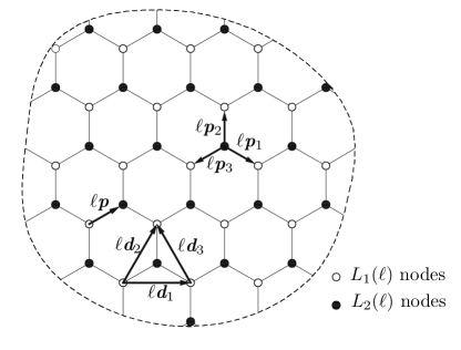
Figure 1: The hexagonal lattice

In (1), $\ell$ denotes the lattice size (the reference interatomic distance), while $\ell\mathbf{d}_{{{}\mathchoice{\mbox{\boldmath$\displaystyle\mathchar 267\relax$}}{\mbox{\boldmath$\textstyle\mathchar 267\relax$}}{\mbox{\boldmath$\scriptstyle\mathchar 267\relax$}}{\mbox{\boldmath$\scriptscriptstyle\mathchar 267\relax$}}}}$ and $\ell\mathbf{p}$ respectively are the lattice vectors and the shift vector, with

$$\mathbf{d}_{1}=\sqrt{3}\mathbf{e}_{1},\quad\mathbf{d}_{2}=\frac{\sqrt{3}}{2}\mathbf{e}_{1}+\frac{3}{2}\mathbf{e}_{2}\quad\mbox{and}\quad\mathbf{p}=\frac{\sqrt{3}}{2}\mathbf{e}_{1}+\frac{1}{2}\mathbf{e}_{2}.$$ (2)

The sides of the hexagonal cells in Figure 1 stand for the bonds between pairs of next nearest neighbor atoms and are represented by the vectors

$$\mathbf{p}_{{}\mathchoice{\mbox{\boldmath$\displaystyle\mathchar 267\relax$}}{\mbox{\boldmath$\textstyle\mathchar 267\relax$}}{\mbox{\boldmath$\scriptstyle\mathchar 267\relax$}}{\mbox{\boldmath$\scriptscriptstyle\mathchar 267\relax$}}}=\mathbf{d}_{{}\mathchoice{\mbox{\boldmath$\displaystyle\mathchar 267\relax$}}{\mbox{\boldmath$\textstyle\mathchar 267\relax$}}{\mbox{\boldmath$\scriptstyle\mathchar 267\relax$}}{\mbox{\boldmath$\scriptscriptstyle\mathchar 267\relax$}}}-\mathbf{p}\ \ ({{}\mathchoice{\mbox{\boldmath$\displaystyle\mathchar 267\relax$}}{\mbox{\boldmath$\textstyle\mathchar 267\relax$}}{\mbox{\boldmath$\scriptstyle\mathchar 267\relax$}}{\mbox{\boldmath$\scriptscriptstyle\mathchar 267\relax$}}}=1,2)\quad\mbox{and}\quad\mathbf{p}_{3}=-\,\mathbf{p}.$$ (3)

For convenience we also set

$$\mathbf{d}_{3}=\mathbf{d}_{2}-\mathbf{d}_{1}.$$

In what follows we denote by

$$\mathbf{x}^{\ell}=n^{1}\ell\mathbf{d}_{1}+n^{2}\ell\mathbf{d}_{2}+m\ell\mathbf{p},\quad(n^{1},n^{2},m)\in\mathbb{Z}^{2}\times\{0,1\}$$ (4)

the lattice points and label them by the triplets $(n^{1},n^{2},m)$: the points with $m=0$ belong to $L_{1}(\ell)$, while those in $L_{2}(\ell)$ correspond to $m=1$.

Graphene energetics depends on the description chosen to mimic atomic interactions. Our model is based on the 2nd-generation Brenner potential [3], which is one of the most used in molecular dynamics simulations of graphene. Accordingly, the binding energy $V$ of an atomic aggregate is given as a sum over nearest neighbors:

$$V=\sum_{i}\sum_{j<i}V_{ij}\,,\quad V_{ij}=V_{R}(l_{ij})+b_{ij}({{}\mathchoice{\mbox{\boldmath$\displaystyle\mathchar 291\relax$}}{\mbox{\boldmath$\textstyle\mathchar 291\relax$}}{\mbox{\boldmath$\scriptstyle\mathchar 291\relax$}}{\mbox{\boldmath$\scriptscriptstyle\mathchar 291\relax$}}}_{hij},\Theta_{hijk})V_{A}(l_{ij}),$$ (5)

where the individual effects of the repulsion and attraction functions $V_{R}(l_{ij})$ and $V_{A}(l_{ij})$, which model pair-wise interactions of the atoms $i$ and $j$ depending on their distance $l_{ij}$, are modulated by the bond-order function $b_{ij}$; for a given bond chain $h,i,j,k$ the function $b_{ij}$ depends in a complex manner on the angle between the edges $hi$ and $ij$ and on the dihedral angle between the planes spanned by $(hi,ij)$ and $(ij,jk)$. This potential reveals that, in order to properly account for the mechanical behavior of graphene, it is necessary to consider three types of energetic contributions:

1. binary interactions between next nearest atoms (edge bonds),

2. three-body interactions between consecutive pairs of next nearest atoms (wedge bonds),

3. and four-body interactions between three consecutive pairs of next nearest atoms (dihedral bonds). There are two types of relevant dihedral bonds: the Z-dihedra, in which the edges connecting the four atoms form a Z-shape, and the C-dihedra, in which the edges form a C-shape (see Fig. 2).

Moreover, it is possible to show [11] that the angle at ease between consecutive edges is greater than $\frac{2}{3}{{}\mathchoice{\mbox{\boldmath$\displaystyle\mathchar 281\relax$}}{\mbox{\boldmath$\textstyle\mathchar 281\relax$}}{\mbox{\boldmath$\scriptstyle\mathchar 281\relax$}}{\mbox{\boldmath$\scriptscriptstyle\mathchar 281\relax$}}}$: this means that in the flat reference configuration the graphene sheet is not stress-free, and we will proper account for this feature.

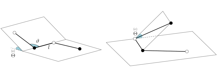
Figure 2: Edge bond $l$, wedge bond $\textstyle\mathchar 291\relax$, Z-dihedron $\operatorname{\overset{(z)}{\Theta}}$ and a C-dihedron $\operatorname{\overset{(c)}{\Theta}}$.

3 Approximated strain measures

In this section we calculate the strain measures associated to a change of configuration described by a displacement field $\mathbf{u}^{\ell}:(L_{1}(\ell)\cup L_{2}(\ell))\cap\Omega\to\mathbb{R}^{3}$. Since we have in mind to deduce a model with the same non-linearities as the Föppl–von Kármán one, we write the displacements of the nodes in the form

$$\mathbf{u}^{\ell}(\mathbf{x}^{\ell})={{}\mathchoice{\mbox{\boldmath$\displaystyle\mathchar 280\relax$}}{\mbox{\boldmath$\textstyle\mathchar 280\relax$}}{\mbox{\boldmath$\scriptstyle\mathchar 280\relax$}}{\mbox{\boldmath$\scriptscriptstyle\mathchar 280\relax$}}}\operatorname{\boldsymbol{\mathfrak{v}}^{\ell}}(\mathbf{x}^{\ell})+{{}\mathchoice{\mbox{\boldmath$\displaystyle\mathchar 280\relax$}}{\mbox{\boldmath$\textstyle\mathchar 280\relax$}}{\mbox{\boldmath$\scriptstyle\mathchar 280\relax$}}{\mbox{\boldmath$\scriptscriptstyle\mathchar 280\relax$}}}^{1/2}\operatorname{\mathfrak{w}^{\ell}}(\mathbf{x}^{\ell})\mathbf{e}_{3},$$ (6)

where $\textstyle\mathchar 280\relax$ is a positive scalar measuring smallness, $\operatorname{\boldsymbol{\mathfrak{v}}^{\ell}}:={{}\mathchoice{\mbox{\boldmath$\displaystyle\mathchar 280\relax$}}{\mbox{\boldmath$\textstyle\mathchar 280\relax$}}{\mbox{\boldmath$\scriptstyle\mathchar 280\relax$}}{\mbox{\boldmath$\scriptscriptstyle\mathchar 280\relax$}}}^{-1}\mathbf{v}^{\ell}:={{}\mathchoice{\mbox{\boldmath$\displaystyle\mathchar 280\relax$}}{\mbox{\boldmath$\textstyle\mathchar 280\relax$}}{\mbox{\boldmath$\scriptstyle\mathchar 280\relax$}}{\mbox{\boldmath$\scriptscriptstyle\mathchar 280\relax$}}}^{-1}(\mathbf{e}_{1}\otimes\mathbf{e}_{1}+\mathbf{e}_{2}\otimes\mathbf{e}_{2})\mathbf{u}^{\ell}$ and $\operatorname{\mathfrak{w}^{\ell}}:={{}\mathchoice{\mbox{\boldmath$\displaystyle\mathchar 280\relax$}}{\mbox{\boldmath$\textstyle\mathchar 280\relax$}}{\mbox{\boldmath$\scriptstyle\mathchar 280\relax$}}{\mbox{\boldmath$\scriptscriptstyle\mathchar 280\relax$}}}^{-1/2}:=w^{\ell}{{}\mathchoice{\mbox{\boldmath$\displaystyle\mathchar 280\relax$}}{\mbox{\boldmath$\textstyle\mathchar 280\relax$}}{\mbox{\boldmath$\scriptstyle\mathchar 280\relax$}}{\mbox{\boldmath$\scriptscriptstyle\mathchar 280\relax$}}}^{-1/2}\mathbf{u}^{\ell}\cdot\mathbf{e}_{3}$ stand for the in-plane and out-of-plane normalized displacements, respectively.

3.1 Change of the edge lengths

With ${{}\mathchoice{\mbox{\boldmath$\displaystyle\mathchar 270\relax$}}{\mbox{\boldmath$\textstyle\mathchar 270\relax$}}{\mbox{\boldmath$\scriptstyle\mathchar 270\relax$}}{\mbox{\boldmath$\scriptscriptstyle\mathchar 270\relax$}}}l_{i}(\mathbf{x}^{\ell})$ we denote the change in length of the edge parallel to $\mathbf{p}_{i}$ and starting from the lattice point $\mathbf{x}^{\ell}\in(L_{1}(\ell)\cup L_{2}(\ell))\cap\Omega$. We fix our attention to lattice points in $L_{2}(\ell)$. Thus,

$${{}\mathchoice{\mbox{\boldmath$\displaystyle\mathchar 270\relax$}}{\mbox{\boldmath$\textstyle\mathchar 270\relax$}}{\mbox{\boldmath$\scriptstyle\mathchar 270\relax$}}{\mbox{\boldmath$\scriptscriptstyle\mathchar 270\relax$}}}l_{i}(\mathbf{x}^{\ell}) =|(\mathbf{x}^{\ell}+\ell\mathbf{p}_{i}+\mathbf{u}^{\ell}(\mathbf{x}^{\ell}+\ell\mathbf{p}_{i}))-(\mathbf{x}^{\ell}+\mathbf{u}^{\ell}(\mathbf{x}^{\ell}))|-\ell$$

$$=\ell|\mathbf{p}_{i}+\frac{\mathbf{u}^{\ell}(\mathbf{x}^{\ell}+\ell\mathbf{p}_{i})-\mathbf{u}^{\ell}(\mathbf{x}^{\ell})}{\ell}|-\ell.$$

On introducing the notation

$$D^{\ell}_{\mathbf{p}_{i}}f(\mathbf{x}):=\frac{f(\mathbf{x}+\ell\mathbf{p}_{i})-f(\mathbf{x})}{\ell},$$ (7)

the axial strain measure can be recast as

$$\frac{{{}\mathchoice{\mbox{\boldmath$\displaystyle\mathchar 270\relax$}}{\mbox{\boldmath$\textstyle\mathchar 270\relax$}}{\mbox{\boldmath$\scriptstyle\mathchar 270\relax$}}{\mbox{\boldmath$\scriptscriptstyle\mathchar 270\relax$}}}\ell_{i}}{\ell_{i}}=|\mathbf{p}_{i}+D^{\ell}_{\mathbf{p}_{i}}\mathbf{u}^{\ell}(\mathbf{x}^{\ell})|-1=|\mathbf{p}_{i}+{{}\mathchoice{\mbox{\boldmath$\displaystyle\mathchar 280\relax$}}{\mbox{\boldmath$\textstyle\mathchar 280\relax$}}{\mbox{\boldmath$\scriptstyle\mathchar 280\relax$}}{\mbox{\boldmath$\scriptscriptstyle\mathchar 280\relax$}}}D^{\ell}_{\mathbf{p}_{i}}\operatorname{\boldsymbol{\mathfrak{v}}^{\ell}}(\mathbf{x}^{\ell})+{{}\mathchoice{\mbox{\boldmath$\displaystyle\mathchar 280\relax$}}{\mbox{\boldmath$\textstyle\mathchar 280\relax$}}{\mbox{\boldmath$\scriptstyle\mathchar 280\relax$}}{\mbox{\boldmath$\scriptscriptstyle\mathchar 280\relax$}}}^{1/2}D^{\ell}_{\mathbf{p}_{i}}\operatorname{\mathfrak{w}^{\ell}}(\mathbf{x}^{\ell})\mathbf{e}_{3}|-1,$$ (8)

where we have made use of (6). The expansion up to the first order in $\textstyle\mathchar 280\relax$ of the non-linear strain measure (8) is

$$\frac{{{}\mathchoice{\mbox{\boldmath$\displaystyle\mathchar 270\relax$}}{\mbox{\boldmath$\textstyle\mathchar 270\relax$}}{\mbox{\boldmath$\scriptstyle\mathchar 270\relax$}}{\mbox{\boldmath$\scriptscriptstyle\mathchar 270\relax$}}}\ell_{i}}{\ell_{i}}={{}\mathchoice{\mbox{\boldmath$\displaystyle\mathchar 280\relax$}}{\mbox{\boldmath$\textstyle\mathchar 280\relax$}}{\mbox{\boldmath$\scriptstyle\mathchar 280\relax$}}{\mbox{\boldmath$\scriptscriptstyle\mathchar 280\relax$}}}\left(D^{\ell}_{\mathbf{p}_{i}}\operatorname{\boldsymbol{\mathfrak{v}}^{\ell}}(\mathbf{x}^{\ell})\cdot\mathbf{p}_{i}+\frac{1}{2}|D^{\ell}_{\mathbf{p}_{i}}\operatorname{\mathfrak{w}^{\ell}}(\mathbf{x}^{\ell})|^{2}\right)+o({{}\mathchoice{\mbox{\boldmath$\displaystyle\mathchar 280\relax$}}{\mbox{\boldmath$\textstyle\mathchar 280\relax$}}{\mbox{\boldmath$\scriptstyle\mathchar 280\relax$}}{\mbox{\boldmath$\scriptscriptstyle\mathchar 280\relax$}}}),$$ (9)

which allows to define the edge strain measure, once rescaled-back by $\textstyle\mathchar 280\relax$:

$${{}\mathchoice{\mbox{\boldmath$\displaystyle\mathchar 290\relax$}}{\mbox{\boldmath$\textstyle\mathchar 290\relax$}}{\mbox{\boldmath$\scriptstyle\mathchar 290\relax$}}{\mbox{\boldmath$\scriptscriptstyle\mathchar 290\relax$}}}_{i}(\mathbf{x}^{\ell}):=D^{\ell}_{\mathbf{p}_{i}}\mathbf{v}^{\ell}(\mathbf{x}^{\ell})\cdot\mathbf{p}_{i}+\frac{1}{2}|D^{\ell}_{\mathbf{p}_{i}}w^{\ell}(\mathbf{x}^{\ell})|^{2}\qquad i=1,2,3,$$ (10)

and ${{}\mathchoice{\mbox{\boldmath$\displaystyle\mathchar 270\relax$}}{\mbox{\boldmath$\textstyle\mathchar 270\relax$}}{\mbox{\boldmath$\scriptstyle\mathchar 270\relax$}}{\mbox{\boldmath$\scriptscriptstyle\mathchar 270\relax$}}}\ell_{i}={{}\mathchoice{\mbox{\boldmath$\displaystyle\mathchar 290\relax$}}{\mbox{\boldmath$\textstyle\mathchar 290\relax$}}{\mbox{\boldmath$\scriptstyle\mathchar 290\relax$}}{\mbox{\boldmath$\scriptscriptstyle\mathchar 290\relax$}}}_{i}\ell_{i}$.

3.2 Change of the wedge angles

For each fixed node $\mathbf{x}^{\ell}\in L_{2}(\ell))\cap\Omega$ we denote by $\operatorname{\overset{(2)}{{{}\mathchoice{\mbox{\boldmath$\displaystyle\mathchar 291\relax$}}{\mbox{\boldmath$\textstyle\mathchar 291\relax$}}{\mbox{\boldmath$\scriptstyle\mathchar 291\relax$}}{\mbox{\boldmath$\scriptscriptstyle\mathchar 291\relax$}}}}}_{i}(\mathbf{x}^{\ell})$ the angle of the wedge delimited by the edges $\mathbf{p}_{i+1}$ and $\mathbf{p}_{i+2}$; that is, the wedge angle opposite to the $i$-th edge (see Fig. 3). Here, $i,i+1$, and $i+2$ take values in $\{1,2,3\}$ and the sums should be interpreted mod 3: for instance, if $i=2$ then $i+1=3$ and $i+2=1$.

Figure 3: The wedge angles $\operatorname{\overset{(2)}{{{}\mathchoice{\mbox{\boldmath$\displaystyle\mathchar 291\relax$}}{\mbox{\boldmath$\textstyle\mathchar 291\relax$}}{\mbox{\boldmath$\scriptstyle\mathchar 291\relax$}}{\mbox{\boldmath$\scriptscriptstyle\mathchar 291\relax$}}}}}_{i}$.

To keep the notation compact, we set

$$\mathbf{u}^{\ell}_{i}:=\mathbf{u}^{\ell}(\mathbf{x}^{\ell}+\ell\mathbf{p}_{i}),\quad\mbox{and}\quad\mathbf{u}^{\ell}_{0}:=\mathbf{u}^{\ell}(\mathbf{x}^{\ell}).$$

Let

$$\mathbf{q}_{i+1}=\ell\left(\mathbf{p}_{i+1}+{{}\mathchoice{\mbox{\boldmath$\displaystyle\mathchar 280\relax$}}{\mbox{\boldmath$\textstyle\mathchar 280\relax$}}{\mbox{\boldmath$\scriptstyle\mathchar 280\relax$}}{\mbox{\boldmath$\scriptscriptstyle\mathchar 280\relax$}}}D^{\ell}_{\mathbf{p}_{i+1}}\operatorname{\boldsymbol{\mathfrak{v}}^{\ell}}(\mathbf{x}^{\ell})+{{}\mathchoice{\mbox{\boldmath$\displaystyle\mathchar 280\relax$}}{\mbox{\boldmath$\textstyle\mathchar 280\relax$}}{\mbox{\boldmath$\scriptstyle\mathchar 280\relax$}}{\mbox{\boldmath$\scriptscriptstyle\mathchar 280\relax$}}}^{1/2}D^{\ell}_{\mathbf{p}_{i+1}}\operatorname{\mathfrak{w}^{\ell}}(\mathbf{x}^{\ell})\mathbf{e}_{3}\right)$$ (11)

and

$$\mathbf{q}_{i+2}=\ell\left(\mathbf{p}_{i+2}+{{}\mathchoice{\mbox{\boldmath$\displaystyle\mathchar 280\relax$}}{\mbox{\boldmath$\textstyle\mathchar 280\relax$}}{\mbox{\boldmath$\scriptstyle\mathchar 280\relax$}}{\mbox{\boldmath$\scriptscriptstyle\mathchar 280\relax$}}}D^{\ell}_{\mathbf{p}_{i+2}}\operatorname{\boldsymbol{\mathfrak{v}}^{\ell}}(\mathbf{x}^{\ell})+{{}\mathchoice{\mbox{\boldmath$\displaystyle\mathchar 280\relax$}}{\mbox{\boldmath$\textstyle\mathchar 280\relax$}}{\mbox{\boldmath$\scriptstyle\mathchar 280\relax$}}{\mbox{\boldmath$\scriptscriptstyle\mathchar 280\relax$}}}^{1/2}D^{\ell}_{\mathbf{p}_{i+2}}\operatorname{\mathfrak{w}^{\ell}}(\mathbf{x}^{\ell})\mathbf{e}_{3}\right)$$ (12)

be the images of the edges parallel to $\mathbf{p}_{i+1}$ and $\mathbf{p}_{i+2}$ and starting at $\mathbf{x}^{\ell}$. Then, the angle $\operatorname{\overset{(2)}{{{}\mathchoice{\mbox{\boldmath$\displaystyle\mathchar 291\relax$}}{\mbox{\boldmath$\textstyle\mathchar 291\relax$}}{\mbox{\boldmath$\scriptstyle\mathchar 291\relax$}}{\mbox{\boldmath$\scriptscriptstyle\mathchar 291\relax$}}}}}_{i}({{}\mathchoice{\mbox{\boldmath$\displaystyle\mathchar 280\relax$}}{\mbox{\boldmath$\textstyle\mathchar 280\relax$}}{\mbox{\boldmath$\scriptstyle\mathchar 280\relax$}}{\mbox{\boldmath$\scriptscriptstyle\mathchar 280\relax$}}})=$ is given by

$$\operatorname{\overset{(2)}{{{}\mathchoice{\mbox{\boldmath$\displaystyle\mathchar 291\relax$}}{\mbox{\boldmath$\textstyle\mathchar 291\relax$}}{\mbox{\boldmath$\scriptstyle\mathchar 291\relax$}}{\mbox{\boldmath$\scriptscriptstyle\mathchar 291\relax$}}}}}_{i}({{}\mathchoice{\mbox{\boldmath$\displaystyle\mathchar 280\relax$}}{\mbox{\boldmath$\textstyle\mathchar 280\relax$}}{\mbox{\boldmath$\scriptstyle\mathchar 280\relax$}}{\mbox{\boldmath$\scriptscriptstyle\mathchar 280\relax$}}})=\arccos\left(\frac{{\mathbf{q}_{i+1}}\cdot{\mathbf{q}_{i+2}}}{|{\mathbf{q}_{i+1}}||{\mathbf{q}_{i+2}}|}\right).$$ (13)

Now, in the light of (11) and (12), we get

$$\frac{1}{\ell^{2}}\mathbf{q}_{i+1}\cdot\mathbf{q}_{i+2}=\mathbf{p}_{i+1}\cdot\mathbf{p}_{i+2}+{{}\mathchoice{\mbox{\boldmath$\displaystyle\mathchar 280\relax$}}{\mbox{\boldmath$\textstyle\mathchar 280\relax$}}{\mbox{\boldmath$\scriptstyle\mathchar 280\relax$}}{\mbox{\boldmath$\scriptscriptstyle\mathchar 280\relax$}}}\Big{(}\mathbf{p}_{i+1}\cdot D^{\ell}_{\mathbf{p}_{i+2}}\operatorname{\boldsymbol{\mathfrak{v}}^{\ell}}(\mathbf{x}^{\ell})+\mathbf{p}_{i+2}\cdot D^{\ell}_{\mathbf{p}_{i+1}}\operatorname{\boldsymbol{\mathfrak{v}}^{\ell}}(\mathbf{x}^{\ell})+D^{\ell}_{\mathbf{p}_{i+1}}\operatorname{\mathfrak{w}^{\ell}}(\mathbf{x}^{\ell})D^{\ell}_{\mathbf{p}_{i+2}}\operatorname{\mathfrak{w}^{\ell}}(\mathbf{x}^{\ell})\Big{)}+o({{}\mathchoice{\mbox{\boldmath$\displaystyle\mathchar 280\relax$}}{\mbox{\boldmath$\textstyle\mathchar 280\relax$}}{\mbox{\boldmath$\scriptstyle\mathchar 280\relax$}}{\mbox{\boldmath$\scriptscriptstyle\mathchar 280\relax$}}}),$$ (14)

and

$$\frac{1}{\ell^{2}}|\mathbf{q}_{i+1}|^{2}=1+{{}\mathchoice{\mbox{\boldmath$\displaystyle\mathchar 280\relax$}}{\mbox{\boldmath$\textstyle\mathchar 280\relax$}}{\mbox{\boldmath$\scriptstyle\mathchar 280\relax$}}{\mbox{\boldmath$\scriptscriptstyle\mathchar 280\relax$}}}\big{(}|D^{\ell}_{\mathbf{p}_{i+1}}\operatorname{\mathfrak{w}^{\ell}}(\mathbf{x}^{\ell})|^{2}+2\mathbf{p}_{i+1}\cdot D^{\ell}_{\mathbf{p}_{i+1}}\operatorname{\boldsymbol{\mathfrak{v}}^{\ell}}(\mathbf{x}^{\ell})\big{)}+o({{}\mathchoice{\mbox{\boldmath$\displaystyle\mathchar 280\relax$}}{\mbox{\boldmath$\textstyle\mathchar 280\relax$}}{\mbox{\boldmath$\scriptstyle\mathchar 280\relax$}}{\mbox{\boldmath$\scriptscriptstyle\mathchar 280\relax$}}}),$$ (15)

$$\frac{1}{\ell^{2}}|\mathbf{q}_{i+2}|^{2}=1+{{}\mathchoice{\mbox{\boldmath$\displaystyle\mathchar 280\relax$}}{\mbox{\boldmath$\textstyle\mathchar 280\relax$}}{\mbox{\boldmath$\scriptstyle\mathchar 280\relax$}}{\mbox{\boldmath$\scriptscriptstyle\mathchar 280\relax$}}}\big{(}|D^{\ell}_{\mathbf{p}_{i+2}}\operatorname{\mathfrak{w}^{\ell}}(\mathbf{x}^{\ell})|^{2}+2\mathbf{p}_{i+2}\cdot D^{\ell}_{\mathbf{p}_{i+2}}\operatorname{\boldsymbol{\mathfrak{v}}^{\ell}}(\mathbf{x}^{\ell})\big{)}+o({{}\mathchoice{\mbox{\boldmath$\displaystyle\mathchar 280\relax$}}{\mbox{\boldmath$\textstyle\mathchar 280\relax$}}{\mbox{\boldmath$\scriptstyle\mathchar 280\relax$}}{\mbox{\boldmath$\scriptscriptstyle\mathchar 280\relax$}}}),$$

so that the expansion up to the first order in $\textstyle\mathchar 280\relax$ of $\operatorname{\overset{(2)}{{{}\mathchoice{\mbox{\boldmath$\displaystyle\mathchar 291\relax$}}{\mbox{\boldmath$\textstyle\mathchar 291\relax$}}{\mbox{\boldmath$\scriptstyle\mathchar 291\relax$}}{\mbox{\boldmath$\scriptscriptstyle\mathchar 291\relax$}}}}}_{i}({{}\mathchoice{\mbox{\boldmath$\displaystyle\mathchar 280\relax$}}{\mbox{\boldmath$\textstyle\mathchar 280\relax$}}{\mbox{\boldmath$\scriptstyle\mathchar 280\relax$}}{\mbox{\boldmath$\scriptscriptstyle\mathchar 280\relax$}}})$ yields

$$\operatorname{\overset{(2)}{{{}\mathchoice{\mbox{\boldmath$\displaystyle\mathchar 291\relax$}}{\mbox{\boldmath$\textstyle\mathchar 291\relax$}}{\mbox{\boldmath$\scriptstyle\mathchar 291\relax$}}{\mbox{\boldmath$\scriptscriptstyle\mathchar 291\relax$}}}}}_{i}({{}\mathchoice{\mbox{\boldmath$\displaystyle\mathchar 280\relax$}}{\mbox{\boldmath$\textstyle\mathchar 280\relax$}}{\mbox{\boldmath$\scriptstyle\mathchar 280\relax$}}{\mbox{\boldmath$\scriptscriptstyle\mathchar 280\relax$}}})=\arccos\left(\frac{\mathbf{p}_{i+1}\cdot\mathbf{p}_{i+2}+a{{}\mathchoice{\mbox{\boldmath$\displaystyle\mathchar 280\relax$}}{\mbox{\boldmath$\textstyle\mathchar 280\relax$}}{\mbox{\boldmath$\scriptstyle\mathchar 280\relax$}}{\mbox{\boldmath$\scriptscriptstyle\mathchar 280\relax$}}}+o({{}\mathchoice{\mbox{\boldmath$\displaystyle\mathchar 280\relax$}}{\mbox{\boldmath$\textstyle\mathchar 280\relax$}}{\mbox{\boldmath$\scriptstyle\mathchar 280\relax$}}{\mbox{\boldmath$\scriptscriptstyle\mathchar 280\relax$}}})}{\sqrt{1+b{{}\mathchoice{\mbox{\boldmath$\displaystyle\mathchar 280\relax$}}{\mbox{\boldmath$\textstyle\mathchar 280\relax$}}{\mbox{\boldmath$\scriptstyle\mathchar 280\relax$}}{\mbox{\boldmath$\scriptscriptstyle\mathchar 280\relax$}}}+o({{}\mathchoice{\mbox{\boldmath$\displaystyle\mathchar 280\relax$}}{\mbox{\boldmath$\textstyle\mathchar 280\relax$}}{\mbox{\boldmath$\scriptstyle\mathchar 280\relax$}}{\mbox{\boldmath$\scriptscriptstyle\mathchar 280\relax$}}})}\,\sqrt{1+c{{}\mathchoice{\mbox{\boldmath$\displaystyle\mathchar 280\relax$}}{\mbox{\boldmath$\textstyle\mathchar 280\relax$}}{\mbox{\boldmath$\scriptstyle\mathchar 280\relax$}}{\mbox{\boldmath$\scriptscriptstyle\mathchar 280\relax$}}}+o({{}\mathchoice{\mbox{\boldmath$\displaystyle\mathchar 280\relax$}}{\mbox{\boldmath$\textstyle\mathchar 280\relax$}}{\mbox{\boldmath$\scriptstyle\mathchar 280\relax$}}{\mbox{\boldmath$\scriptscriptstyle\mathchar 280\relax$}}})}}\right)=\frac{2}{3}{{}\mathchoice{\mbox{\boldmath$\displaystyle\mathchar 281\relax$}}{\mbox{\boldmath$\textstyle\mathchar 281\relax$}}{\mbox{\boldmath$\scriptstyle\mathchar 281\relax$}}{\mbox{\boldmath$\scriptscriptstyle\mathchar 281\relax$}}}-\frac{1}{2\sqrt{3}}(4a+b+c)\,{{}\mathchoice{\mbox{\boldmath$\displaystyle\mathchar 280\relax$}}{\mbox{\boldmath$\textstyle\mathchar 280\relax$}}{\mbox{\boldmath$\scriptstyle\mathchar 280\relax$}}{\mbox{\boldmath$\scriptscriptstyle\mathchar 280\relax$}}}+o({{}\mathchoice{\mbox{\boldmath$\displaystyle\mathchar 280\relax$}}{\mbox{\boldmath$\textstyle\mathchar 280\relax$}}{\mbox{\boldmath$\scriptstyle\mathchar 280\relax$}}{\mbox{\boldmath$\scriptscriptstyle\mathchar 280\relax$}}}),$$ (16)

with

$$a:=\mathbf{p}_{i+1}\cdot D^{\ell}_{\mathbf{p}_{i+2}}\operatorname{\boldsymbol{\mathfrak{v}}^{\ell}}(\mathbf{x}^{\ell})+\mathbf{p}_{i+2}\cdot D^{\ell}_{\mathbf{p}_{i+1}}\operatorname{\boldsymbol{\mathfrak{v}}^{\ell}}(\mathbf{x}^{\ell})+D^{\ell}_{\mathbf{p}_{i+1}}\operatorname{\mathfrak{w}^{\ell}}(\mathbf{x}^{\ell})D^{\ell}_{\mathbf{p}_{i+2}}\operatorname{\mathfrak{w}^{\ell}}(\mathbf{x}^{\ell}),$$ (17)

$$b:=|D^{\ell}_{\mathbf{p}_{i+1}}\operatorname{\mathfrak{w}^{\ell}}(\mathbf{x}^{\ell})|^{2}+2\mathbf{p}_{i+1}\cdot D^{\ell}_{\mathbf{p}_{i+1}}\operatorname{\boldsymbol{\mathfrak{v}}^{\ell}}(\mathbf{x}^{\ell}),$$

$$c:=|D^{\ell}_{\mathbf{p}_{i+2}}\operatorname{\mathfrak{w}^{\ell}}(\mathbf{x}^{\ell})|^{2}+2\mathbf{p}_{i+2}\cdot D^{\ell}_{\mathbf{p}_{i+2}}\operatorname{\boldsymbol{\mathfrak{v}}^{\ell}}(\mathbf{x}^{\ell}).$$

This allows to define the wedge strain measure, once the displacement is rescaled-back by $\textstyle\mathchar 280\relax$:

$$\operatorname{\overset{(2)}{{{}\mathchoice{\mbox{\boldmath$\displaystyle\mathchar 288\relax$}}{\mbox{\boldmath$\textstyle\mathchar 288\relax$}}{\mbox{\boldmath$\scriptstyle\mathchar 288\relax$}}{\mbox{\boldmath$\scriptscriptstyle\mathchar 288\relax$}}}}}_{i}(\mathbf{x}^{\ell})=\operatorname{\overset{(2)}{{{}\mathchoice{\mbox{\boldmath$\displaystyle\mathchar 291\relax$}}{\mbox{\boldmath$\textstyle\mathchar 291\relax$}}{\mbox{\boldmath$\scriptstyle\mathchar 291\relax$}}{\mbox{\boldmath$\scriptscriptstyle\mathchar 291\relax$}}}}}_{i}-\frac{2}{3}{{}\mathchoice{\mbox{\boldmath$\displaystyle\mathchar 281\relax$}}{\mbox{\boldmath$\textstyle\mathchar 281\relax$}}{\mbox{\boldmath$\scriptstyle\mathchar 281\relax$}}{\mbox{\boldmath$\scriptscriptstyle\mathchar 281\relax$}}}=\\ -\frac{1}{\sqrt{3}}\Bigg{(}D^{\ell}_{\mathbf{p}_{i+1}}\mathbf{v}^{\ell}(\mathbf{x}^{\ell})\cdot\mathbf{p}_{i+1}+D^{\ell}_{\mathbf{p}_{i+2}}\mathbf{v}^{\ell}(\mathbf{x}^{\ell})\cdot\mathbf{p}_{i+2}+2(D^{\ell}_{\mathbf{p}_{i+1}}\mathbf{v}^{\ell}(\mathbf{x}^{\ell})\cdot\mathbf{p}_{i+2}+D^{\ell}_{\mathbf{p}_{i+2}}\mathbf{v}^{\ell}(\mathbf{x}^{\ell})\cdot\mathbf{p}_{i+1})+\\ \frac{1}{2}\left(|D^{\ell}_{\mathbf{p}_{i+1}}w^{\ell}(\mathbf{x}^{\ell})|^{2}+|D^{\ell}_{\mathbf{p}_{i+2}}w^{\ell}(\mathbf{x}^{\ell})|^{2}\right)+2D^{\ell}_{\mathbf{p}_{i+1}}w^{\ell}(\mathbf{x}^{\ell})\,D^{\ell}_{\mathbf{p}_{i+2}}w^{\ell}(\mathbf{x}^{\ell})\Bigg{)}\,,$$ (18)

for $\mathbf{x}^{\ell}\in L_{2}(\ell))\cap\Omega$. In particular, algebraic manipulations allow to conclude that

$$\sum_{i=1}^{3}\operatorname{\overset{(2)}{{{}\mathchoice{\mbox{\boldmath$\displaystyle\mathchar 288\relax$}}{\mbox{\boldmath$\textstyle\mathchar 288\relax$}}{\mbox{\boldmath$\scriptstyle\mathchar 288\relax$}}{\mbox{\boldmath$\scriptscriptstyle\mathchar 288\relax$}}}}}_{i}(\mathbf{x}^{\ell})=-3\sqrt{3}\Bigg{(}\frac{1}{3}\sum_{i=1}^{3}D^{\ell}_{\mathbf{p}_{i}}w^{\ell}(\mathbf{x}^{\ell})\Bigg{)}^{2}.$$ (19)

If we consider a lattice point belonging to $L_{1}(\ell)$, it is not difficult to see that

$$\overset{(1)}{{{}\mathchoice{\mbox{\boldmath$\displaystyle\mathchar 288\relax$}}{\mbox{\boldmath$\textstyle\mathchar 288\relax$}}{\mbox{\boldmath$\scriptstyle\mathchar 288\relax$}}{\mbox{\boldmath$\scriptscriptstyle\mathchar 288\relax$}}}}_{i}(\mathbf{x}^{\ell})=\frac{1}{\sqrt{3}}\Bigg{(}D^{\ell}_{-\mathbf{p}_{i+1}}\mathbf{v}^{\ell}(\mathbf{x}^{\ell})\cdot\mathbf{p}_{i+1}+D^{\ell}_{-\mathbf{p}_{i+2}}\mathbf{v}^{\ell}(\mathbf{x}^{\ell})\cdot\mathbf{p}_{i+2}+2(D^{\ell}_{-\mathbf{p}_{i+1}}\mathbf{v}^{\ell}(\mathbf{x}^{\ell})\cdot\mathbf{p}_{i+2}+D^{\ell}_{-\mathbf{p}_{i+2}}\mathbf{v}^{\ell}(\mathbf{x}^{\ell})\cdot\mathbf{p}_{i+1})+\\ -\frac{1}{2}\left(|D^{\ell}_{-\mathbf{p}_{i+1}}w^{\ell}(\mathbf{x}^{\ell})|^{2}+|D^{\ell}_{-\mathbf{p}_{i+2}}w^{\ell}(\mathbf{x}^{\ell})|^{2}\right)-2D^{\ell}_{-\mathbf{p}_{i+1}}w^{\ell}(\mathbf{x}^{\ell})\,D^{\ell}_{-\mathbf{p}_{i+2}}w^{\ell}(\mathbf{x}^{\ell})\Bigg{)}\,.$$ (20)

3.3 Change of the dihedral angles

For each fixed node $\mathbf{x}^{\ell}\in L_{2}(\ell)\cap\Omega$ and for each edge parallel to $\mathbf{p}_{i}$ and starting at $\mathbf{x}^{\ell}$ we need to define four types of dihedral angles $\operatorname{\overset{(c)}{\Theta}}_{\mathbf{p}_{i}^{+}}(\mathbf{x}^{\ell}),\operatorname{\overset{(c)}{\Theta}}_{\mathbf{p}_{i}^{-}}(\mathbf{x}^{\ell}),\operatorname{\overset{(z)}{\Theta}}_{\mathbf{p}_{i}\mathbf{p}_{i+1}}(\mathbf{x}^{\ell})$ and $\operatorname{\overset{(z)}{\Theta}}_{\mathbf{p}_{i}\mathbf{p}_{i+2}}(\mathbf{x}^{\ell})$:

$$\cos\operatorname{\overset{(c)}{\Theta}}_{\mathbf{p}_{i}^{+}}=\frac{(\mathbf{q}_{i}\times\mathbf{q}_{i+1})\cdot(\mathbf{q}_{i}\times\mathbf{q}_{i^{+}})}{|\mathbf{q}_{i}\times\mathbf{q}_{i+1}||\mathbf{q}_{i}\times\mathbf{q}_{i^{+}}|},$$ (21)

$$\cos\operatorname{\overset{(c)}{\Theta}}_{\mathbf{p}_{i}^{-}}=\frac{(\mathbf{q}_{i+2}\times\mathbf{q}_{i})\cdot(\mathbf{q}_{i^{-}}\times\mathbf{q}_{i})}{|\mathbf{q}_{i+2}\times\mathbf{q}_{i}||\mathbf{q}_{i^{-}}\times\mathbf{q}_{i})|},$$

$$\cos\operatorname{\overset{(z)}{\Theta}}_{\mathbf{p}_{i}\mathbf{p}_{i+1}}=\frac{(\mathbf{q}_{i}\times\mathbf{q}_{i+1})\cdot(\mathbf{q}_{i^{-}}\times\mathbf{q}_{i})}{|\mathbf{q}_{i}\times\mathbf{q}_{i+1}||\mathbf{q}_{i^{-}}\times\mathbf{q}_{i}|},$$

$$\cos\operatorname{\overset{(z)}{\Theta}}_{\mathbf{p}_{i}\mathbf{p}_{i+2}}=\frac{(\mathbf{q}_{i+2}\times\mathbf{q}_{i})\cdot(\mathbf{q}_{i}\times\mathbf{q}_{i^{+}})}{|\mathbf{q}_{i+2}\times\mathbf{q}_{i}||\mathbf{q}_{i}\times\mathbf{q}_{i^{+}}|},$$

where

$$\mathbf{q}_{i^{+}}= \mathbf{x}^{\ell}+\ell\mathbf{p}_{i}-\ell\mathbf{p}_{i+2}+\mathbf{u}^{\ell}(\mathbf{x}^{\ell}+\ell\mathbf{p}_{i}-\ell\mathbf{p}_{i+2})-\big{(}\mathbf{x}^{\ell}+\ell\mathbf{p}_{i}+\mathbf{u}^{\ell}(\mathbf{x}^{\ell}+\ell\mathbf{p}_{i})\big{)}$$ (22)

$$= -\ell\mathbf{p}_{i+2}+\mathbf{u}^{\ell}_{i^{+}}-\mathbf{u}^{\ell}_{i},\qquad\qquad\mathbf{u}^{\ell}_{i^{+}}:=\mathbf{u}^{\ell}(\mathbf{x}^{\ell}+\ell\mathbf{p}_{i}-\ell\mathbf{p}_{i+2}),$$

$$\mathbf{q}_{i^{-}}= \mathbf{x}^{\ell}+\ell\mathbf{p}_{i}-\ell\mathbf{p}_{i+1}+\mathbf{u}^{\ell}(\mathbf{x}^{\ell}+\ell\mathbf{p}_{i}-\ell\mathbf{p}_{i+1})-\big{(}\mathbf{x}^{\ell}+\ell\mathbf{p}_{i}+\mathbf{u}^{\ell}(\mathbf{x}^{\ell}+\ell\mathbf{p}_{i})\big{)}$$

$$= -\ell\mathbf{p}_{i+1}+\mathbf{u}^{\ell}_{i^{-}}-\mathbf{u}^{\ell}_{i},\qquad\qquad\mathbf{u}^{\ell}_{i^{-}}:=\mathbf{u}^{\ell}(\mathbf{x}^{\ell}+\ell\mathbf{p}_{i}-\ell\mathbf{p}_{i+1})$$

are the images of vectors $\ell\mathbf{p}_{i^{+}}$ and $\ell\mathbf{p}_{i^{-}}$ (see Fig. 4, for $i=1$), parallel to $\mathbf{p}_{i+2}$ and $\mathbf{p}_{i+1}$ and starting at the image of the point $\mathbf{x}^{\ell}+\ell\mathbf{p}_{i}$.

Also here, $i,i+1$, and $i+2$ take values in $\{1,2,3\}$ and the sums should be interpreted mod 3: for instance, if $i=3$ then $i+1=1$ and $i+2=2$.

The C-dihedral angle $\operatorname{\overset{(c)}{\Theta}}_{\mathbf{p}_{i}^{+}}(\mathbf{x}^{\ell})$ is the angle corresponding to the C-dihedron with middle edge $\ell\mathbf{p}_{i}$ and oriented as $\mathbf{p}_{i}^{\perp}$, while $\operatorname{\overset{(c)}{\Theta}}_{\mathbf{p}_{i}^{-}}(\mathbf{x}^{\ell})$ is the angle corresponding to the C-dihedron oriented opposite to $\mathbf{p}_{i}^{\perp}$ (see Fig. 4 for $i=1$). The Z-dihedral angle $\operatorname{\overset{(z)}{\Theta}}_{\mathbf{p}_{i}\mathbf{p}_{i+1}}(\mathbf{x}^{\ell})$ corresponds to the Z-dihedron with middle edge $\ell\mathbf{p}_{i}$ and the other two edges parallel to $\mathbf{p}_{i+1}$ (see Fig. 4 for $i=1$).

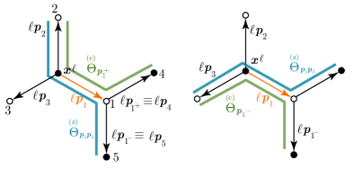
Figure 4: Left: C-dihedral angles $\operatorname{\overset{(c)}{\Theta}}_{\mathbf{p}_{1}^{+}}$ (green) and Z-dihedral angle $\operatorname{\overset{(z)}{\Theta}}_{\mathbf{p}_{1}\mathbf{p}_{2}}$ (blue). Right: C-dihedral angles $\operatorname{\overset{(c)}{\Theta}}_{\mathbf{p}_{1}^{-}}$ (green) and Z-dihedral angle $\operatorname{\overset{(z)}{\Theta}}_{\mathbf{p}_{1}\mathbf{p}_{3}}$ (blue).

To fix the ideas, we focus on the dihedral angle $\operatorname{\overset{(z)}{\Theta}}_{\mathbf{p}_{1}\mathbf{p}_{2}}$, sketched in Fig. 4; the other strains can be obtained in analogous manner.

The first order approximation of the dihedral angle is all we need to evaluate the corresponding energy contribution.

Let us introduce the vector

$$\mathbf{q}_{5}=\ell\mathbf{p}_{5}+(\operatorname{\boldsymbol{\mathfrak{v}}^{\ell}}_{5}-\operatorname{\boldsymbol{\mathfrak{v}}^{\ell}}_{1}){{}\mathchoice{\mbox{\boldmath$\displaystyle\mathchar 280\relax$}}{\mbox{\boldmath$\textstyle\mathchar 280\relax$}}{\mbox{\boldmath$\scriptstyle\mathchar 280\relax$}}{\mbox{\boldmath$\scriptscriptstyle\mathchar 280\relax$}}}+\operatorname{\mathfrak{w}^{\ell}}_{5}{{}\mathchoice{\mbox{\boldmath$\displaystyle\mathchar 280\relax$}}{\mbox{\boldmath$\textstyle\mathchar 280\relax$}}{\mbox{\boldmath$\scriptstyle\mathchar 280\relax$}}{\mbox{\boldmath$\scriptscriptstyle\mathchar 280\relax$}}}^{1/2},$$

image of $\mathbf{p}_{5}$ under the deformation. We have that

$$\operatorname{\overset{(z)}{\Theta}}_{\mathbf{p}_{1}\mathbf{p}_{2}}=\arccos\left(\frac{\mathbf{q}_{1}\times\mathbf{q}_{2}}{|\mathbf{q}_{1}\times\mathbf{q}_{2}|}\cdot\frac{\mathbf{q}_{5}\times\mathbf{q}_{1}}{|\mathbf{q}_{5}\times\mathbf{q}_{1}|}\right).$$ (23)

Cumbersome computations yield:

$$\frac{\mathbf{q}_{1}\times\mathbf{q}_{2}}{|\mathbf{q}_{1}\times\mathbf{q}_{2}|}\cdot\frac{\mathbf{q}_{5}\times\mathbf{q}_{1}}{|\mathbf{q}_{5}\times\mathbf{q}_{1}|}=1-\frac{2}{3\ell^{2}}(\operatorname{\mathfrak{w}^{\ell}}_{5}-\operatorname{\mathfrak{w}^{\ell}}_{1}+\operatorname{\mathfrak{w}^{\ell}}_{2}-\operatorname{\mathfrak{w}^{\ell}}_{0})^{2}{{}\mathchoice{\mbox{\boldmath$\displaystyle\mathchar 280\relax$}}{\mbox{\boldmath$\textstyle\mathchar 280\relax$}}{\mbox{\boldmath$\scriptstyle\mathchar 280\relax$}}{\mbox{\boldmath$\scriptscriptstyle\mathchar 280\relax$}}}+o({{}\mathchoice{\mbox{\boldmath$\displaystyle\mathchar 280\relax$}}{\mbox{\boldmath$\textstyle\mathchar 280\relax$}}{\mbox{\boldmath$\scriptstyle\mathchar 280\relax$}}{\mbox{\boldmath$\scriptscriptstyle\mathchar 280\relax$}}}).$$ (24)

The expansion up to the first order in $\textstyle\mathchar 280\relax$ of $\operatorname{\overset{(z)}{\Theta}}_{\mathbf{p}_{1}\mathbf{p}_{2}}$ yields

$$\operatorname{\overset{(z)}{\Theta}}_{\mathbf{p}_{1}\mathbf{p}_{2}}({{}\mathchoice{\mbox{\boldmath$\displaystyle\mathchar 280\relax$}}{\mbox{\boldmath$\textstyle\mathchar 280\relax$}}{\mbox{\boldmath$\scriptstyle\mathchar 280\relax$}}{\mbox{\boldmath$\scriptscriptstyle\mathchar 280\relax$}}})=\arccos\Big{(}1-a^{2}{{}\mathchoice{\mbox{\boldmath$\displaystyle\mathchar 280\relax$}}{\mbox{\boldmath$\textstyle\mathchar 280\relax$}}{\mbox{\boldmath$\scriptstyle\mathchar 280\relax$}}{\mbox{\boldmath$\scriptscriptstyle\mathchar 280\relax$}}}+o({{}\mathchoice{\mbox{\boldmath$\displaystyle\mathchar 280\relax$}}{\mbox{\boldmath$\textstyle\mathchar 280\relax$}}{\mbox{\boldmath$\scriptstyle\mathchar 280\relax$}}{\mbox{\boldmath$\scriptscriptstyle\mathchar 280\relax$}}})\big{)}=\sqrt{2}a\,{{}\mathchoice{\mbox{\boldmath$\displaystyle\mathchar 280\relax$}}{\mbox{\boldmath$\textstyle\mathchar 280\relax$}}{\mbox{\boldmath$\scriptstyle\mathchar 280\relax$}}{\mbox{\boldmath$\scriptscriptstyle\mathchar 280\relax$}}}^{1/2}+O({{}\mathchoice{\mbox{\boldmath$\displaystyle\mathchar 280\relax$}}{\mbox{\boldmath$\textstyle\mathchar 280\relax$}}{\mbox{\boldmath$\scriptstyle\mathchar 280\relax$}}{\mbox{\boldmath$\scriptscriptstyle\mathchar 280\relax$}}}^{3/2}),\quad a^{2}:=\frac{2}{3\ell^{2}}(\operatorname{\mathfrak{w}^{\ell}}_{5}-\operatorname{\mathfrak{w}^{\ell}}_{1}+\operatorname{\mathfrak{w}^{\ell}}_{2}-\operatorname{\mathfrak{w}^{\ell}}_{0})^{2}.$$ (25)

This allows to define the Z-dihedron strain measure, once the displacement be rescaled-back by $\textstyle\mathchar 280\relax$:

$$\operatorname{\overset{(z)}{\Psi}}_{\mathbf{p}_{1}\mathbf{p}_{2}}=\operatorname{\overset{(z)}{\Theta}}_{\mathbf{p}_{1}\mathbf{p}_{2}}({{}\mathchoice{\mbox{\boldmath$\displaystyle\mathchar 280\relax$}}{\mbox{\boldmath$\textstyle\mathchar 280\relax$}}{\mbox{\boldmath$\scriptstyle\mathchar 280\relax$}}{\mbox{\boldmath$\scriptscriptstyle\mathchar 280\relax$}}})-\arccos\left(\frac{\mathbf{p}_{1}\times\mathbf{p}_{2}}{|\mathbf{p}_{1}\times\mathbf{p}_{2}|}\cdot\frac{\mathbf{p}_{5}\times\mathbf{p}_{1}}{|\mathbf{p}_{5}\times\mathbf{p}_{1}|}\right)=\frac{2\sqrt{3}}{3\ell}\Big{(}w^{\ell}_{5}-w^{\ell}_{1}+w^{\ell}_{2}-w^{\ell}_{0}\Big{)}.$$ (26)

For a generic Z-dihedral angle centered in $\mathbf{p}_{i}$, we get

$$\operatorname{\overset{(z)}{\Psi}}_{\mathbf{p}_{i}\mathbf{p}_{i+1}}(\mathbf{x}^{\ell})=\frac{2\sqrt{3}}{3\ell}[w^{\ell}(\mathbf{x}^{\ell}+\ell\mathbf{p}_{i}-\ell\mathbf{p}_{i+1})-w^{\ell}(\mathbf{x}^{\ell}+\ell\mathbf{p}_{i})+w^{\ell}(\mathbf{x}^{\ell}+\ell\mathbf{p}_{i+1})-w^{\ell}(\mathbf{x}^{\ell})],$$ (27)

$$\operatorname{\overset{(z)}{\Psi}}_{\mathbf{p}_{i}\mathbf{p}_{i+2}}(\mathbf{x}^{\ell})=\frac{2\sqrt{3}}{3\ell}[w^{\ell}(\mathbf{x}^{\ell}+\ell\mathbf{p}_{i}-\ell\mathbf{p}_{i+2})-w^{\ell}(\mathbf{x}^{\ell}+\ell\mathbf{p}_{i})+w^{\ell}(\mathbf{x}^{\ell}+\ell\mathbf{p}_{i+2})-w^{\ell}(\mathbf{x}^{\ell})].$$

Analogous computations allows to determine the C-dihedron strain measure

$$\operatorname{\overset{(c)}{\Psi}}_{\mathbf{p}_{i}^{+}}(\mathbf{x}^{\ell})=\frac{2\sqrt{3}}{3\ell}[2w^{\ell}(\mathbf{x}^{\ell})-w^{\ell}(\mathbf{x}^{\ell}+\ell\mathbf{p}_{i+1})+w^{\ell}(\mathbf{x}^{\ell}+\ell\mathbf{p}_{i}-\ell\mathbf{p}_{i+2})-2w^{\ell}(\mathbf{x}^{\ell}+\ell\mathbf{p}_{i})],$$ (28)

$$\operatorname{\overset{(c)}{\Psi}}_{\mathbf{p}_{i}^{-}}(\mathbf{x}^{\ell})=-\frac{2\sqrt{3}}{3\ell}[2w^{\ell}(\mathbf{x}^{\ell})-w^{\ell}(\mathbf{x}^{\ell}+\ell\mathbf{p}_{i+2})+w^{\ell}(\mathbf{x}^{\ell}+\ell\mathbf{p}_{i}-\ell\mathbf{p}_{i+1})-2w^{\ell}(\mathbf{x}^{\ell}+\ell\mathbf{p}_{i})].$$

4 Membrane and bending energy

The above calculations show that $\textstyle\mathchar 290\relax$ and $\textstyle\mathchar 288\relax$ depend upon both the in-plane and the out-of-plane components of $\mathbf{u}^{\ell}$, while $\operatorname{\overset{(c)}{\Psi}}$, and $\operatorname{\overset{(z)}{\Psi}}$ depend upon the out-of-plane component of $\mathbf{u}^{\ell}$; moreover, (19) shows that the sum of all $\textstyle\mathchar 288\relax$ depends on the out-of-plane component of $\mathbf{u}^{\ell}$. We introduce the following splitting of the energy into membrane and bending parts:

$$\mathcal{U}_{\ell}=\mathcal{U}_{\ell}^{(m)}+\mathcal{U}_{\ell}^{(b)},\quad\mathcal{U}_{\ell}^{(m)}:=\mathcal{U}_{\ell}^{(e)}+\mathcal{U}_{\ell}^{(w)}\quad\mathcal{U}_{\ell}^{(b)}:=\mathcal{U}_{\ell}^{(s)}+\mathcal{U}_{\ell}^{(d)}$$

defined by

$$\mathcal{U}_{\ell}^{(e)}:=\frac{1}{2}\,\sum_{\mathcal{E}}k^{l}({{}\mathchoice{\mbox{\boldmath$\displaystyle\mathchar 270\relax$}}{\mbox{\boldmath$\textstyle\mathchar 270\relax$}}{\mbox{\boldmath$\scriptstyle\mathchar 270\relax$}}{\mbox{\boldmath$\scriptscriptstyle\mathchar 270\relax$}}}\ell)^{2}=\frac{1}{2}\,\sum_{\mathcal{E}}k^{l}\ell^{2}{{}\mathchoice{\mbox{\boldmath$\displaystyle\mathchar 290\relax$}}{\mbox{\boldmath$\textstyle\mathchar 290\relax$}}{\mbox{\boldmath$\scriptstyle\mathchar 290\relax$}}{\mbox{\boldmath$\scriptscriptstyle\mathchar 290\relax$}}}^{2}$$ (29)

$$\mathcal{U}_{\ell}^{(w)}:=\frac{1}{2}\,\sum_{\mathcal{W}}k^{{}\mathchoice{\mbox{\boldmath$\displaystyle\mathchar 291\relax$}}{\mbox{\boldmath$\textstyle\mathchar 291\relax$}}{\mbox{\boldmath$\scriptstyle\mathchar 291\relax$}}{\mbox{\boldmath$\scriptscriptstyle\mathchar 291\relax$}}}\ell^{2}\,{{}\mathchoice{\mbox{\boldmath$\displaystyle\mathchar 288\relax$}}{\mbox{\boldmath$\textstyle\mathchar 288\relax$}}{\mbox{\boldmath$\scriptstyle\mathchar 288\relax$}}{\mbox{\boldmath$\scriptscriptstyle\mathchar 288\relax$}}}^{2}$$

$$\mathcal{U}_{\ell}^{(s)}:={{}\mathchoice{\mbox{\boldmath$\displaystyle\mathchar 284\relax$}}{\mbox{\boldmath$\textstyle\mathchar 284\relax$}}{\mbox{\boldmath$\scriptstyle\mathchar 284\relax$}}{\mbox{\boldmath$\scriptscriptstyle\mathchar 284\relax$}}}_{0}\sum_{\mathcal{W}}{{}\mathchoice{\mbox{\boldmath$\displaystyle\mathchar 288\relax$}}{\mbox{\boldmath$\textstyle\mathchar 288\relax$}}{\mbox{\boldmath$\scriptstyle\mathchar 288\relax$}}{\mbox{\boldmath$\scriptscriptstyle\mathchar 288\relax$}}},$$

$$\mathcal{U}_{\ell}^{(d)}:=\frac{1}{2}\,\sum_{\mathcal{Z}}k^{\mathcal{Z}}\,\operatorname{\overset{(z)}{\Psi}}^{2}+\frac{1}{2}\,\sum_{\mathcal{C}}k^{\mathcal{C}}\,\operatorname{\overset{(c)}{\Psi}}^{2},$$

where $\mathcal{U}_{\ell}^{(e)}$, $\mathcal{U}_{\ell}^{(w)}$, $\mathcal{U}_{\ell}^{(s)}$ and $\mathcal{U}_{\ell}^{(d)}$ are the edge, wedge, self-, and dihedral energy, respectively.

The self-stress term is the outcome of the fact that the angle at ease between consecutive edges is greater than $\frac{2}{3}{{}\mathchoice{\mbox{\boldmath$\displaystyle\mathchar 281\relax$}}{\mbox{\boldmath$\textstyle\mathchar 281\relax$}}{\mbox{\boldmath$\scriptstyle\mathchar 281\relax$}}{\mbox{\boldmath$\scriptscriptstyle\mathchar 281\relax$}}}$: this means that in the flat reference configuration the graphene sheet is not stress-free, and ${{}\mathchoice{\mbox{\boldmath$\displaystyle\mathchar 284\relax$}}{\mbox{\boldmath$\textstyle\mathchar 284\relax$}}{\mbox{\boldmath$\scriptstyle\mathchar 284\relax$}}{\mbox{\boldmath$\scriptscriptstyle\mathchar 284\relax$}}}_{0}$ represents the pre-stress couple (see [11]). The constants $k^{l}$, $k^{{}\mathchoice{\mbox{\boldmath$\displaystyle\mathchar 291\relax$}}{\mbox{\boldmath$\textstyle\mathchar 291\relax$}}{\mbox{\boldmath$\scriptstyle\mathchar 291\relax$}}{\mbox{\boldmath$\scriptscriptstyle\mathchar 291\relax$}}}$, $k^{\mathcal{Z}}$, and $k^{\mathcal{C}}$ can be deduced by means of the 2nd-generation Brenner potential. In the wedge energy we may interpret the presence of $\ell^{2}$ as a scaling of the constant $k^{{}\mathchoice{\mbox{\boldmath$\displaystyle\mathchar 291\relax$}}{\mbox{\boldmath$\textstyle\mathchar 291\relax$}}{\mbox{\boldmath$\scriptstyle\mathchar 291\relax$}}{\mbox{\boldmath$\scriptscriptstyle\mathchar 291\relax$}}}$, introduced to keep the energy finite as the lattice size $\ell$ goes to zero. We notice that the multiplication factor $\ell^{2}$ appears in all contributions to the membrane energy.

With the notation introduced in Section 3 we now write the energy more explicitly. The edge energy can be written as

$$\mathcal{U}_{\ell}^{(e)}=\frac{1}{2}\,k^{l}\ell^{2}\sum_{\mathbf{x}^{\ell}\in L_{2}(\ell)\cap\Omega}\sum_{i=1}^{3}{{}\mathchoice{\mbox{\boldmath$\displaystyle\mathchar 290\relax$}}{\mbox{\boldmath$\textstyle\mathchar 290\relax$}}{\mbox{\boldmath$\scriptstyle\mathchar 290\relax$}}{\mbox{\boldmath$\scriptscriptstyle\mathchar 290\relax$}}}_{i}^{2}(\mathbf{x}^{\ell}),$$ (30)

while the wedge energy reads:

$$\mathcal{U}_{\ell}^{(w)}=\frac{1}{2}\,k^{{{}\mathchoice{\mbox{\boldmath$\displaystyle\mathchar 291\relax$}}{\mbox{\boldmath$\textstyle\mathchar 291\relax$}}{\mbox{\boldmath$\scriptstyle\mathchar 291\relax$}}{\mbox{\boldmath$\scriptscriptstyle\mathchar 291\relax$}}}}\ell^{2}\sum_{\mathbf{x}^{\ell}\in L_{1}(\ell)\cap\Omega}\sum_{i=1}^{3}\overset{(1)}{{{}\mathchoice{\mbox{\boldmath$\displaystyle\mathchar 288\relax$}}{\mbox{\boldmath$\textstyle\mathchar 288\relax$}}{\mbox{\boldmath$\scriptstyle\mathchar 288\relax$}}{\mbox{\boldmath$\scriptscriptstyle\mathchar 288\relax$}}}}_{i}{}^{2}(\mathbf{x}^{\ell})+\frac{1}{2}\,k^{{{}\mathchoice{\mbox{\boldmath$\displaystyle\mathchar 291\relax$}}{\mbox{\boldmath$\textstyle\mathchar 291\relax$}}{\mbox{\boldmath$\scriptstyle\mathchar 291\relax$}}{\mbox{\boldmath$\scriptscriptstyle\mathchar 291\relax$}}}}\ell^{2}\sum_{\mathbf{x}^{\ell}\in L_{2}(\ell)\cap\Omega}\sum_{i=1}^{3}\overset{(2)}{{{}\mathchoice{\mbox{\boldmath$\displaystyle\mathchar 288\relax$}}{\mbox{\boldmath$\textstyle\mathchar 288\relax$}}{\mbox{\boldmath$\scriptstyle\mathchar 288\relax$}}{\mbox{\boldmath$\scriptscriptstyle\mathchar 288\relax$}}}}_{i}{}^{2}(\mathbf{x}^{\ell}).$$ (31)

Analogously, the self-energy becomes

$$\mathcal{U}^{(s)}_{\ell}=\sum_{\mathbf{x}^{\ell}\in L_{1}(\ell)\cap\Omega}{{}\mathchoice{\mbox{\boldmath$\displaystyle\mathchar 284\relax$}}{\mbox{\boldmath$\textstyle\mathchar 284\relax$}}{\mbox{\boldmath$\scriptstyle\mathchar 284\relax$}}{\mbox{\boldmath$\scriptscriptstyle\mathchar 284\relax$}}}_{0}\sum_{i=1}^{3}\overset{(1)}{{{}\mathchoice{\mbox{\boldmath$\displaystyle\mathchar 288\relax$}}{\mbox{\boldmath$\textstyle\mathchar 288\relax$}}{\mbox{\boldmath$\scriptstyle\mathchar 288\relax$}}{\mbox{\boldmath$\scriptscriptstyle\mathchar 288\relax$}}}}_{i}(\mathbf{x}^{\ell})+\sum_{\mathbf{x}^{\ell}\in L_{2}(\ell)\cap\Omega}{{}\mathchoice{\mbox{\boldmath$\displaystyle\mathchar 284\relax$}}{\mbox{\boldmath$\textstyle\mathchar 284\relax$}}{\mbox{\boldmath$\scriptstyle\mathchar 284\relax$}}{\mbox{\boldmath$\scriptscriptstyle\mathchar 284\relax$}}}_{0}\sum_{i=1}^{3}\overset{(2)}{{{}\mathchoice{\mbox{\boldmath$\displaystyle\mathchar 288\relax$}}{\mbox{\boldmath$\textstyle\mathchar 288\relax$}}{\mbox{\boldmath$\scriptstyle\mathchar 288\relax$}}{\mbox{\boldmath$\scriptscriptstyle\mathchar 288\relax$}}}}_{i}(\mathbf{x}^{\ell}).$$ (32)

We further split the dihedral energy $\mathcal{U}_{\ell}^{(d)}$ in

$$\mathcal{U}_{\ell}^{(d)}:=\mathcal{U}^{\mathcal{Z}}_{\ell}+\mathcal{U}^{\mathcal{C}}_{\ell},$$

where

$$\mathcal{U}^{\mathcal{Z}}_{\ell}=\frac{1}{2}\,k^{\mathcal{Z}}\sum_{\mathbf{x}^{\ell}\in L_{2}(\ell)\cap\Omega}\sum_{i=1}^{3}\Bigg{(}\operatorname{\overset{(z)}{\Psi}}_{\mathbf{p}_{i}\mathbf{p}_{i+2}}(\mathbf{x}^{\ell})\Bigg{)}^{2}+\Bigg{(}\operatorname{\overset{(z)}{\Psi}}_{\mathbf{p}_{i}\mathbf{p}_{i+1}}(\mathbf{x}^{\ell})\Bigg{)}^{2}$$ (33)

is the contribution of the Z-dihedra, and

$$\mathcal{U}^{\mathcal{C}}_{\ell}=\frac{1}{2}k^{\mathcal{C}}\,\sum_{\mathbf{x}^{\ell}\in L_{2}(\ell)\cap\Omega}\sum_{i=1}^{3}\Bigg{(}\operatorname{\overset{(c)}{\Psi}}_{\mathbf{p}_{i}^{+}}(\mathbf{x}^{\ell})\Bigg{)}^{2}+\Bigg{(}\operatorname{\overset{(c)}{\Psi}}_{\mathbf{p}_{i}^{-}}(\mathbf{x}^{\ell})\Bigg{)}^{2}$$ (34)

is the contribution of the C-dihedra.

We notice that the bending energy here obtained is the same as [5, 8]. In the following, we then focus on the membrane energy.

5 The continuum limit of the membrane energy

In the previous sections the discrete energy $\mathcal{U}_{\ell}$ was defined over the lattice $(L_{1}(\ell)\cup L_{2}(\ell))\cap\Omega$. By letting the lattice size $\ell$ go to zero the discrete set $(L_{1}(\ell)\cup L_{2}(\ell))\cap\Omega$ invades the domain $\Omega$, and the displacement functions $w^{\ell}$ and $\mathbf{v}^{\ell}$ will approach two functions $w$ and $\mathbf{v}$ defined over $\Omega$. To derive a continuous energy, defined over the domain $\Omega$, from the discrete energy $\mathcal{U}_{\ell}$ we need to specify the relations between $w^{\ell}$ and $w$ and between $\mathbf{v}^{\ell}$ and $\mathbf{v}$.

We assume $w:\Omega\to\mathbb{R}$ to be twice continuously differentiable and to, almost, coincide with ${w}^{\ell}$ over the lattice $(L_{1}(\ell)\cup L_{2}(\ell))\cap\Omega$. More precisely, we assume that

$${w}^{\ell}(\mathbf{x}^{\ell})=w(\mathbf{x}^{\ell})+o(\ell),\qquad\forall\mathbf{x}^{\ell}\in(L_{1}(\ell)\cup L_{2}(\ell))\cap\Omega.$$ (35)

If we think of $w$ and ${w}^{\ell}$ as the macroscopic and microscopic displacements, respectively, then (35) can be thought as a Cauchy–Born rule. The assumption (35) is motivated and essentially justified in [8].

For the in-plane displacement we assume $\mathbf{v}:\Omega\to\mathbb{R}^{2}$ to be continuously differentiable and

$$\mathbf{v}^{\ell}(\mathbf{x}^{\ell}) =\mathbf{v}(\mathbf{x}^{\ell})+o(\ell), \forall \mathbf{x}^{\ell}\in L_{1}(\ell)\cap\Omega,$$ (36)

$$\mathbf{v}^{\ell}(\mathbf{x}^{\ell}) =\mathbf{v}(\mathbf{x}^{\ell})-\ell\mathbf{s}(\mathbf{x}^{\ell})+o(\ell),\qquad \forall \mathbf{x}^{\ell}\in L_{2}(\ell)\cap\Omega.$$

Thus, over the lattice $L_{1}(\ell)$ we make the Cauchy–Born assumption for the in-plane displacement, while over the lattice $L_{2}(\ell)$ this assumption is relaxed by introducing a “shift displacement” $\mathbf{s}:\Omega\to\mathbb{R}^{2}$ that we assume to be continuously differentiable. Clearly, if the shift displacement is set equal to zero we have the Cauchy–Born rule over both lattices, but energetically it might be convenient to have a shift displacement $\mathbf{s}$ different from zero. The minus sign in front of the term containing $\mathbf{s}$ is introduced simply for later convenience. The assumption (36) is motivated and essentially justified in [4].

We note that for $\mathbf{x}^{\ell}\in L_{2}(\ell)$ we have that $\mathbf{x}^{\ell}+\ell\mathbf{p}_{i}\in L_{1}(\ell)$, for $i=1,2,3$, and

$$\mathbf{v}^{\ell}(\mathbf{x}^{\ell}+\ell\mathbf{p}_{i})=\mathbf{v}(\mathbf{x}^{\ell}+\ell\mathbf{p}_{i})+o(\ell)=\mathbf{v}(\mathbf{x}^{\ell})+\ell\nabla\mathbf{v}(\mathbf{x}^{\ell})\mathbf{p}_{i}+o(\ell)=\mathbf{v}^{\ell}(\mathbf{x}^{\ell})+\ell\mathbf{s}(\mathbf{x}^{\ell})+\ell\nabla\mathbf{v}(\mathbf{x}^{\ell})\mathbf{p}_{i}+o(\ell),$$

while for $\mathbf{x}^{\ell}\in L_{1}(\ell)$ we have that $\mathbf{x}^{\ell}-\ell\mathbf{p}_{i}\in L_{1}(\ell)$, for $i=1,2,3$, and

$$\mathbf{v}^{\ell}(\mathbf{x}^{\ell}-\ell\mathbf{p}_{i}) =\mathbf{v}(\mathbf{x}^{\ell}-\ell\mathbf{p}_{i})-\ell\mathbf{s}(\mathbf{x}^{\ell}-\ell\mathbf{p}_{i})+o(\ell)=\mathbf{v}(\mathbf{x}^{\ell})-\ell\nabla\mathbf{v}(\mathbf{x}^{\ell})\mathbf{p}_{i}-\ell\mathbf{s}(\mathbf{x}^{\ell})+o(\ell)$$ (37)

$$=\mathbf{v}^{\ell}(\mathbf{x}^{\ell})-\ell\nabla\mathbf{v}(\mathbf{x}^{\ell})\mathbf{p}_{i}-\ell\mathbf{s}(\mathbf{x}^{\ell})+o(\ell).$$ (38)

Thus,

$$D^{\ell}_{\mathbf{p}_{i}}\mathbf{v}^{\ell}(\mathbf{x}^{\ell}) =\frac{\mathbf{v}^{\ell}(\mathbf{x}^{\ell}+\ell\mathbf{p}_{i})-\mathbf{v}^{\ell}(\mathbf{x}^{\ell})}{\ell}=\nabla\mathbf{v}(\mathbf{x}^{\ell})\mathbf{p}_{i}+\mathbf{s}(\mathbf{x}^{\ell})+o(1), \mathbf{x}^{\ell}\in L_{2}(\ell),$$ (39)

$$D^{\ell}_{-\mathbf{p}_{i}}\mathbf{v}^{\ell}(\mathbf{x}^{\ell}) =\frac{\mathbf{v}^{\ell}(\mathbf{x}^{\ell}-\ell\mathbf{p}_{i})-\mathbf{v}^{\ell}(\mathbf{x}^{\ell})}{\ell}=-\nabla\mathbf{v}(\mathbf{x}^{\ell})\mathbf{p}_{i}-\mathbf{s}(\mathbf{x}^{\ell})+o(1), \mathbf{x}^{\ell}\in L_{1}(\ell),$$

and similarly for $\mathbf{x}^{\ell}\in L_{2}(\ell)$ we have that

$$D^{\ell}_{\mathbf{p}_{i}}{w}^{\ell}(\mathbf{x}^{\ell})=\frac{{w}^{\ell}(\mathbf{x}^{\ell}+\ell\mathbf{p}_{i})-{w}^{\ell}(\mathbf{x}^{\ell})}{\ell}=\nabla w(\mathbf{x}^{\ell})\cdot\mathbf{p}_{i}+o(1).$$ (40)

For $i=1,2,3$ and for $\mathbf{x}^{\ell}\in L_{2}(\ell)$ the edge strain measure defined in (45) writes as

$${{}\mathchoice{\mbox{\boldmath$\displaystyle\mathchar 290\relax$}}{\mbox{\boldmath$\textstyle\mathchar 290\relax$}}{\mbox{\boldmath$\scriptstyle\mathchar 290\relax$}}{\mbox{\boldmath$\scriptscriptstyle\mathchar 290\relax$}}}_{i}(\mathbf{x}^{\ell}) =\mathbf{p}_{i}\cdot D^{\ell}_{\mathbf{p}_{i}}\mathbf{v}^{\ell}(\mathbf{x}^{\ell})+\frac{1}{2}|D^{\ell}_{\mathbf{p}_{i}}w(\mathbf{x}^{\ell})|^{2}$$ (41)

$$=\nabla\mathbf{v}(\mathbf{x}^{\ell})\mathbf{p}_{i}\cdot\mathbf{p}_{i}+\mathbf{s}(\mathbf{x}^{\ell})\cdot\mathbf{p}_{i}+\frac{1}{2}|\nabla w(\mathbf{x}^{\ell})\cdot\mathbf{p}_{i}|^{2}+o(1)$$ (42)

$$=\mathbf{E}\mathbf{v}(\mathbf{x}^{\ell})\mathbf{p}_{i}\cdot\mathbf{p}_{i}+\mathbf{s}(\mathbf{x}^{\ell})\cdot\mathbf{p}_{i}+\frac{1}{2}|\nabla w(\mathbf{x}^{\ell})\cdot\mathbf{p}_{i}|^{2}+o(1)$$ (43)

$$=[\mathbf{E}\mathbf{v}(\mathbf{x}^{\ell})+\frac{1}{2}\nabla w(\mathbf{x}^{\ell})\otimes\nabla w(\mathbf{x}^{\ell})]\cdot\mathbf{p}_{i}\otimes\mathbf{p}_{i}+\mathbf{s}(\mathbf{x}^{\ell})\cdot\mathbf{p}_{i}+o(1)$$ (44)

$$=\mathbf{E}^{\rm vk}[\mathbf{v},w](\mathbf{x}^{\ell})\cdot\mathbf{p}_{i}\otimes\mathbf{p}_{i}+\mathbf{s}(\mathbf{x}^{\ell})\cdot\mathbf{p}_{i}+o(1)$$ (45)

where

$$\mathbf{E}\mathbf{v}:=\frac{\nabla\mathbf{v}+(\nabla\mathbf{v})^{T}}{2},\qquad\mathbf{E}^{\rm vk}[\mathbf{v},w]:=\mathbf{E}\mathbf{v}+\frac{1}{2}\nabla w\otimes\nabla w,$$

are the linearized and the von Kármán strain tensors, respectively. Similarly, the wedge strain measure defined in (18) rewrites as

$$\operatorname{\overset{(2)}{{{}\mathchoice{\mbox{\boldmath$\displaystyle\mathchar 288\relax$}}{\mbox{\boldmath$\textstyle\mathchar 288\relax$}}{\mbox{\boldmath$\scriptstyle\mathchar 288\relax$}}{\mbox{\boldmath$\scriptscriptstyle\mathchar 288\relax$}}}}}_{i}(\mathbf{x}^{\ell}) =\frac{-1}{\sqrt{3}}\Big{(}\big{(}\nabla\mathbf{v}(\mathbf{x}^{\ell})\mathbf{p}_{i+1}+\mathbf{s}(\mathbf{x}^{\ell})\big{)}\cdot\mathbf{p}_{i+1}+\big{(}\nabla\mathbf{v}(\mathbf{x}^{\ell})\mathbf{p}_{i+2}+\mathbf{s}(\mathbf{x}^{\ell})\big{)}\cdot\mathbf{p}_{i+2}$$ (46)

$$\hskip 28.45274pt+2\big{(}\nabla\mathbf{v}(\mathbf{x}^{\ell})\mathbf{p}_{i+1}+\mathbf{s}(\mathbf{x}^{\ell})\big{)}\cdot\mathbf{p}_{i+2}+2\big{(}\nabla\mathbf{v}(\mathbf{x}^{\ell})\mathbf{p}_{i+2}+\mathbf{s}(\mathbf{x}^{\ell})\big{)}\cdot\mathbf{p}_{i+1}$$ (47)

$$\hskip 28.45274pt+\frac{1}{2}\left(|\nabla w(\mathbf{x}^{\ell})\cdot\mathbf{p}_{i+1}|^{2}+|\nabla w(\mathbf{x}^{\ell})\cdot\mathbf{p}_{i+2}|^{2}\right)+2\nabla w(\mathbf{x}^{\ell})\cdot\mathbf{p}_{i+1}\,\nabla w(\mathbf{x}^{\ell})\cdot\mathbf{p}_{i+2}\Big{)}+o(1)$$ (48)

$$=\frac{-1}{\sqrt{3}}\Big{(}\mathbf{E}\mathbf{v}(\mathbf{x}^{\ell})\mathbf{p}_{i+1}\cdot\mathbf{p}_{i+1}+\mathbf{E}\mathbf{v}(\mathbf{x}^{\ell})\mathbf{p}_{i+2}\cdot\mathbf{p}_{i+2}+4\mathbf{E}\mathbf{v}(\mathbf{x}^{\ell})\mathbf{p}_{i+1}\cdot\mathbf{p}_{i+2}$$ (49)

$$\hskip 28.45274pt+3\mathbf{s}(\mathbf{x}^{\ell})\big{)}\cdot(\mathbf{p}_{i+1}+\mathbf{p}_{i+2})$$ (50)

$$\hskip 28.45274pt+\frac{1}{2}\nabla w(\mathbf{x}^{\ell})\otimes\nabla w(\mathbf{x}^{\ell})\cdot\big{(}\mathbf{p}_{i+1}\otimes\mathbf{p}_{i+1}+\mathbf{p}_{i+2}\otimes\mathbf{p}_{i+2}+4\mathbf{p}_{i+1}\otimes\mathbf{p}_{i+2}\big{)}\Big{)}+o(1)$$ (51)

$$=\frac{-1}{\sqrt{3}}\Big{(}\mathbf{E}^{\rm vk}[\mathbf{v},w](\mathbf{x}^{\ell})\cdot\mathbf{P}_{i}-3\mathbf{s}(\mathbf{x}^{\ell})\cdot\mathbf{p}_{i}\Big{)}+o(1),$$ (52)

where we set

$$\mathbf{P}_{i}:=\mathbf{p}_{i+1}\otimes\mathbf{p}_{i+1}+\mathbf{p}_{i+2}\otimes\mathbf{p}_{i+2}+2\mathbf{p}_{i+1}\otimes\mathbf{p}_{i+2}+2\mathbf{p}_{i+2}\otimes\mathbf{p}_{i+1},$$ (53)

and where we used the fact that $\mathbf{p}_{i+1}+\mathbf{p}_{i+2}=-\mathbf{p}_{i}$. A similar computation shows that, see (20),

$$\overset{(1)}{{{}\mathchoice{\mbox{\boldmath$\displaystyle\mathchar 288\relax$}}{\mbox{\boldmath$\textstyle\mathchar 288\relax$}}{\mbox{\boldmath$\scriptstyle\mathchar 288\relax$}}{\mbox{\boldmath$\scriptscriptstyle\mathchar 288\relax$}}}}_{i}(\mathbf{x}^{\ell})=\frac{-1}{\sqrt{3}}\Big{(}\mathbf{E}^{\rm vk}[\mathbf{v},w](\mathbf{x}^{\ell})\cdot\mathbf{P}_{i}-3\mathbf{s}(\mathbf{x}^{\ell})\cdot\mathbf{p}_{i}\Big{)}+o(1).$$ (54)

We now compute the energies. The edge energy (30) becomes

$$\mathcal{U}_{\ell}^{(e)} =\frac{1}{2}\,k^{l}\ell^{2}\sum_{\mathbf{x}^{\ell}\in L_{2}(\ell)\cap\Omega}\sum_{i=1}^{3}\Big{(}\mathbf{E}^{\rm vk}[\mathbf{v},w](\mathbf{x}^{\ell})\cdot\mathbf{p}_{i}\otimes\mathbf{p}_{i}+\mathbf{s}(\mathbf{x}^{\ell})\cdot\mathbf{p}_{i}+o(1)\Big{)}^{2}$$ (55)

$$=o(1)+\frac{1}{2}\,k^{l}\ell^{2}\sum_{\mathbf{x}^{\ell}\in L_{2}(\ell)\cap\Omega}\sum_{i=1}^{3}\Big{(}\mathbf{E}^{\rm vk}[\mathbf{v},w](\mathbf{x}^{\ell})\cdot\mathbf{p}_{i}\otimes\mathbf{p}_{i}+\mathbf{s}(\mathbf{x}^{\ell})\cdot\mathbf{p}_{i}\Big{)}^{2},$$ (56)

where the second equality is obtained by noticing that the number of points $\mathbf{x}^{\ell}$ in $L_{2}(\ell)\cap\Omega$ is of order $1/\ell^{2}$. Let $|E^{\ell}(\mathbf{x}^{\ell})|=\ell^{2}3\sqrt{3}/2$ be the area of the hexagon $E^{\ell}(\mathbf{x}^{\ell})$ of side $\ell$ centred at $\mathbf{x}^{\ell}$, see Figure 6, and let ${{}\mathchoice{\mbox{\boldmath$\displaystyle\mathchar 287\relax$}}{\mbox{\boldmath$\textstyle\mathchar 287\relax$}}{\mbox{\boldmath$\scriptstyle\mathchar 287\relax$}}{\mbox{\boldmath$\scriptscriptstyle\mathchar 287\relax$}}}_{E^{\ell}(\mathbf{x}^{\ell})}(\mathbf{x})$ be the characteristic function of $E^{\ell}(\mathbf{x}^{\ell})$, i.e., the function equal to $1$ if $\mathbf{x}\in E^{\ell}(\mathbf{x}^{\ell})$ and $0$ otherwise. The energy $\mathcal{U}_{\ell}^{(e)}$ may be rewritten as

$$\mathcal{U}_{\ell}^{(e)} =o(1)+\frac{k^{l}}{3\sqrt{3}}\,\sum_{i=1}^{3}\int_{\Omega}\sum_{\mathbf{x}^{\ell}\in L_{2}(\ell)\cap\Omega}\Big{(}\mathbf{E}^{\rm vk}[\mathbf{v},w](\mathbf{x}^{\ell})\cdot\mathbf{p}_{i}\otimes\mathbf{p}_{i}+\mathbf{s}(\mathbf{x}^{\ell})\cdot\mathbf{p}_{i}\Big{)}^{2}{{}\mathchoice{\mbox{\boldmath$\displaystyle\mathchar 287\relax$}}{\mbox{\boldmath$\textstyle\mathchar 287\relax$}}{\mbox{\boldmath$\scriptstyle\mathchar 287\relax$}}{\mbox{\boldmath$\scriptscriptstyle\mathchar 287\relax$}}}_{E^{\ell}(\mathbf{x}^{\ell})}(\mathbf{x})\,d\mathbf{x}$$ (57)

and since the function $\sum_{\mathbf{x}^{\ell}\in L_{2}(\ell)\cap\Omega}\big{(}\mathbf{E}^{\rm vk}[\mathbf{v},w](\mathbf{x}^{\ell})\cdot\mathbf{p}_{i}\otimes\mathbf{p}_{i}+\mathbf{s}(\mathbf{x}^{\ell})\cdot\mathbf{p}_{i}\big{)}^{2}{{}\mathchoice{\mbox{\boldmath$\displaystyle\mathchar 287\relax$}}{\mbox{\boldmath$\textstyle\mathchar 287\relax$}}{\mbox{\boldmath$\scriptstyle\mathchar 287\relax$}}{\mbox{\boldmath$\scriptscriptstyle\mathchar 287\relax$}}}_{E^{\ell}(\mathbf{x}^{\ell})}(\mathbf{x})$ converges, as $\ell$ goes to zero, to $\big{(}\mathbf{E}^{\rm vk}[\mathbf{v},w](\mathbf{x})\cdot\mathbf{p}_{i}\otimes\mathbf{p}_{i}+\mathbf{s}(\mathbf{x})\cdot\mathbf{p}_{i}\big{)}^{2}$ we have that

$$\lim_{\ell\to 0}\mathcal{U}_{\ell}^{(e)}=\frac{k^{l}}{3\sqrt{3}}\,\sum_{i=1}^{3}\int_{\Omega}\big{(}\mathbf{E}^{\rm vk}[\mathbf{v},w](\mathbf{x})\cdot\mathbf{p}_{i}\otimes\mathbf{p}_{i}+\mathbf{s}(\mathbf{x})\cdot\mathbf{p}_{i}\big{)}^{2}\,d\mathbf{x}=:\mathcal{U}_{0\mathbf{s}}^{(e)}(\mathbf{v},w,\mathbf{s}).$$ (58)

By taking into account that the expression for $\overset{(1)}{{{}\mathchoice{\mbox{\boldmath$\displaystyle\mathchar 288\relax$}}{\mbox{\boldmath$\textstyle\mathchar 288\relax$}}{\mbox{\boldmath$\scriptstyle\mathchar 288\relax$}}{\mbox{\boldmath$\scriptscriptstyle\mathchar 288\relax$}}}}_{i}$ and $\overset{(2)}{{{}\mathchoice{\mbox{\boldmath$\displaystyle\mathchar 288\relax$}}{\mbox{\boldmath$\textstyle\mathchar 288\relax$}}{\mbox{\boldmath$\scriptstyle\mathchar 288\relax$}}{\mbox{\boldmath$\scriptscriptstyle\mathchar 288\relax$}}}}_{i}$ are identical, the wedge energy (31) rewrites:

$$\mathcal{U}_{\ell}^{(w)}=o(1)+\frac{1}{2}\,k^{{{}\mathchoice{\mbox{\boldmath$\displaystyle\mathchar 291\relax$}}{\mbox{\boldmath$\textstyle\mathchar 291\relax$}}{\mbox{\boldmath$\scriptstyle\mathchar 291\relax$}}{\mbox{\boldmath$\scriptscriptstyle\mathchar 291\relax$}}}}\ell^{2}\sum_{\mathbf{x}^{\ell}\in(L_{1}(\ell)\cup L_{2}(\ell))\cap\Omega}\sum_{i=1}^{3}\frac{1}{{3}}\big{(}\mathbf{E}^{\rm vk}[\mathbf{v},w](\mathbf{x}^{\ell})\cdot\mathbf{P}_{i}-3\mathbf{s}(\mathbf{x}^{\ell})\cdot\mathbf{p}_{i}\big{)}^{2}$$ (59)

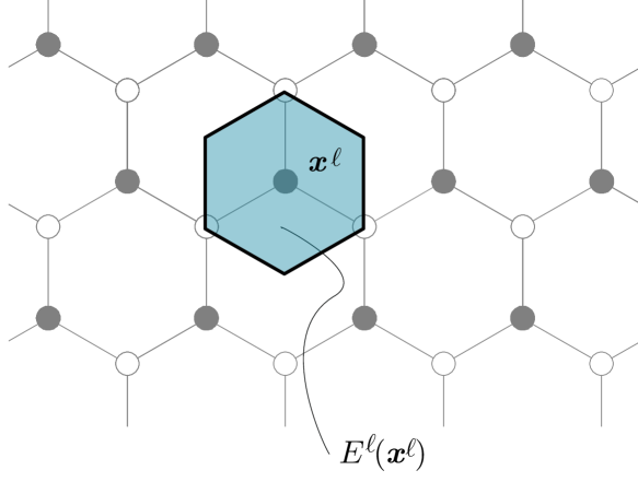
Figure 5: The hexagon $E^{\ell}(\mathbf{x}^{\ell})$.

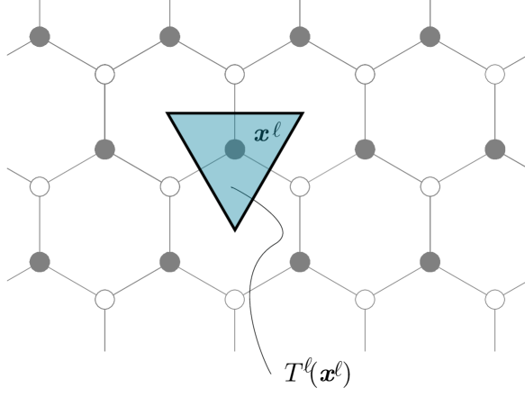
Figure 6: The triangle $T^{\ell}(\mathbf{x}^{\ell})$

By introducing the triangles $T^{\ell}(\mathbf{x}^{\ell})$ centered at $\mathbf{x}^{\ell}$ of area $3\sqrt{3}\ell^{2}/4$ as depicted in Figure 6 and proceeding as above, we deduce that

$$\lim_{\ell\to 0}\mathcal{U}_{\ell}^{(w)}=\frac{2k^{{{}\mathchoice{\mbox{\boldmath$\displaystyle\mathchar 291\relax$}}{\mbox{\boldmath$\textstyle\mathchar 291\relax$}}{\mbox{\boldmath$\scriptstyle\mathchar 291\relax$}}{\mbox{\boldmath$\scriptscriptstyle\mathchar 291\relax$}}}}}{9\sqrt{3}}\,\sum_{i=1}^{3}\int_{\Omega}\big{(}\mathbf{E}^{\rm vk}[\mathbf{v},w](\mathbf{x})\cdot\mathbf{P}_{i}-3\mathbf{s}(\mathbf{x})\cdot\mathbf{p}_{i}\big{)}^{2}\,d\mathbf{x}=:\mathcal{U}_{0\mathbf{s}}^{(w)}(\mathbf{v},w,\mathbf{s}).$$ (60)

The limit of the membrane energy is

$$\mathcal{U}_{0\mathbf{s}}^{(m)}(\mathbf{v},w,\mathbf{s}) :=\lim_{\ell\to 0}\mathcal{U}_{\ell}^{(m)}=\mathcal{U}_{0\mathbf{s}}^{(e)}(\mathbf{v},w,\mathbf{s})+\mathcal{U}_{0\mathbf{s}}^{(w)}(\mathbf{v},w,\mathbf{s})$$ (61)

$$=\frac{k^{l}}{3\sqrt{3}}\,\sum_{i=1}^{3}\int_{\Omega}\big{(}\mathbf{E}^{\rm vk}[\mathbf{v},w](\mathbf{x})\cdot\mathbf{p}_{i}\otimes\mathbf{p}_{i}+\mathbf{s}(\mathbf{x})\cdot\mathbf{p}_{i}\big{)}^{2}\,d\mathbf{x}$$ (62)

$$\hskip 28.45274pt+\frac{2k^{{{}\mathchoice{\mbox{\boldmath$\displaystyle\mathchar 291\relax$}}{\mbox{\boldmath$\textstyle\mathchar 291\relax$}}{\mbox{\boldmath$\scriptstyle\mathchar 291\relax$}}{\mbox{\boldmath$\scriptscriptstyle\mathchar 291\relax$}}}}}{9\sqrt{3}}\,\sum_{i=1}^{3}\int_{\Omega}\big{(}\mathbf{E}^{\rm vk}[\mathbf{v},w](\mathbf{x})\cdot\mathbf{P}_{i}-3\mathbf{s}(\mathbf{x})\cdot\mathbf{p}_{i}\big{)}^{2}\,d\mathbf{x}$$ (63)

$$=\int_{\Omega}\sum_{i=1}^{3}\Big{(}\frac{k^{l}}{3\sqrt{3}}(\mathbf{E}^{\rm vk}[\mathbf{v},w](\mathbf{x})\cdot\mathbf{p}_{i}\otimes\mathbf{p}_{i})^{2}+\frac{2k^{{{}\mathchoice{\mbox{\boldmath$\displaystyle\mathchar 291\relax$}}{\mbox{\boldmath$\textstyle\mathchar 291\relax$}}{\mbox{\boldmath$\scriptstyle\mathchar 291\relax$}}{\mbox{\boldmath$\scriptscriptstyle\mathchar 291\relax$}}}}}{9\sqrt{3}}(\mathbf{E}^{\rm vk}[\mathbf{v},w](\mathbf{x})\cdot\mathbf{P}_{i})^{2}\Big{)}$$ (64)

$$\hskip 39.83385pt+\mathbf{s}\cdot\sum_{i=1}^{3}\Big{(}\frac{2k^{l}}{3\sqrt{3}}\mathbf{E}^{\rm vk}[\mathbf{v},w](\mathbf{x})\cdot\mathbf{p}_{i}\otimes\mathbf{p}_{i}-\frac{4k^{{{}\mathchoice{\mbox{\boldmath$\displaystyle\mathchar 291\relax$}}{\mbox{\boldmath$\textstyle\mathchar 291\relax$}}{\mbox{\boldmath$\scriptstyle\mathchar 291\relax$}}{\mbox{\boldmath$\scriptscriptstyle\mathchar 291\relax$}}}}}{3\sqrt{3}}\mathbf{E}^{\rm vk}[\mathbf{v},w](\mathbf{x})\cdot\mathbf{P}_{i}\Big{)}\mathbf{p}_{i}$$ (65)

$$\hskip 39.83385pt+(\frac{k^{l}}{3\sqrt{3}}+\frac{2k^{{{}\mathchoice{\mbox{\boldmath$\displaystyle\mathchar 291\relax$}}{\mbox{\boldmath$\textstyle\mathchar 291\relax$}}{\mbox{\boldmath$\scriptstyle\mathchar 291\relax$}}{\mbox{\boldmath$\scriptscriptstyle\mathchar 291\relax$}}}}}{\sqrt{3}})\sum_{i=1}^{3}(\mathbf{s}(\mathbf{x})\cdot\mathbf{p}_{i}\big{)}^{2}\,d\mathbf{x}$$ (66)

By using the relations

$$\mathbf{p}_{1}=\frac{\sqrt{3}}{2}\mathbf{e}_{1}-\frac{1}{2}\mathbf{e}_{2},\qquad\mathbf{p}_{2}=\mathbf{e}_{2},\qquad\mathbf{p}_{3}=-\frac{\sqrt{3}}{2}\mathbf{e}_{1}-\frac{1}{2}\mathbf{e}_{2}$$ (68)

we find that

$$\mathbf{E}^{\rm vk}\,\mathbf{p}_{1}\cdot\mathbf{p}_{1} =\frac{3}{4}(\mathbf{E}^{\rm vk})_{11}+\frac{1}{4}(\mathbf{E}^{\rm vk})_{22}-\frac{\sqrt{3}}{2}(\mathbf{E}^{\rm vk})_{12},$$ (69)

$$\mathbf{E}^{\rm vk}\,\mathbf{p}_{2}\cdot\mathbf{p}_{2} =(\mathbf{E}^{\rm vk})_{22},$$ (70)

$$\mathbf{E}^{\rm vk}\,\mathbf{p}_{3}\cdot\mathbf{p}_{3} =\frac{3}{4}(\mathbf{E}^{\rm vk})_{11}+\frac{1}{4}(\mathbf{E}^{\rm vk})_{22}+\frac{\sqrt{3}}{2}(\mathbf{E}^{\rm vk})_{12},$$ (71)

where $(\mathbf{E}^{\rm vk})_{{{}\mathchoice{\mbox{\boldmath$\displaystyle\mathchar 267\relax$}}{\mbox{\boldmath$\textstyle\mathchar 267\relax$}}{\mbox{\boldmath$\scriptstyle\mathchar 267\relax$}}{\mbox{\boldmath$\scriptscriptstyle\mathchar 267\relax$}}}{{}\mathchoice{\mbox{\boldmath$\displaystyle\mathchar 268\relax$}}{\mbox{\boldmath$\textstyle\mathchar 268\relax$}}{\mbox{\boldmath$\scriptstyle\mathchar 268\relax$}}{\mbox{\boldmath$\scriptscriptstyle\mathchar 268\relax$}}}}$ are the components of $\mathbf{E}^{\rm vk}=\mathbf{E}^{\rm vk}[\mathbf{v},w]$ with respect to the basis $\{\mathbf{e}_{i}\}$. A simple computation then shows that

$$\sum_{i=1}^{3}(\mathbf{E}^{\rm vk}\,\mathbf{p}_{i}\cdot\mathbf{p}_{i})^{2} =\frac{1}{8}\Big{(}9(\mathbf{E}^{\rm vk})_{11}^{2}+9(\mathbf{E}^{\rm vk})_{22}^{2}+6(\mathbf{E}^{\rm vk})_{11}(\mathbf{E}^{\rm vk})_{22}+12(\mathbf{E}\mathbf{v})_{12}^{2}\Big{)},$$ (72)

$$=\frac{3}{8}\Big{(}3(\operatorname{\textrm{tr}}\mathbf{E}^{\rm vk})^{2}-4\det\mathbf{E}^{\rm vk}\Big{)}.$$ (73)

Similarly we find

$$\sum_{i=1}^{3}(\mathbf{E}^{\rm vk}\cdot\mathbf{P}_{i})^{2}=\frac{27}{8}\Big{(}(\operatorname{\textrm{tr}}\mathbf{E}^{\rm vk})^{2}-4\det\mathbf{E}^{\rm vk}\Big{)},$$ (74)

$$\sum_{i=1}^{3}(\mathbf{E}^{\rm vk}\cdot\mathbf{p}_{i}\otimes\mathbf{p}_{i})\mathbf{p}_{i},=-\frac{3}{2}(\mathbf{E}^{\rm vk})_{12}\mathbf{e}_{1}-\frac{3}{4}\big{(}(\mathbf{E}^{\rm vk})_{11}-(\mathbf{E}^{\rm vk})_{22}\big{)}\mathbf{e}_{2},$$ (75)

$$\sum_{i=1}^{3}(\mathbf{E}^{\rm vk}\cdot\mathbf{P}_{i})\mathbf{p}_{i}=-\frac{9}{2}(\mathbf{E}^{\rm vk})_{12}\mathbf{e}_{1}-\frac{9}{4}\big{(}(\mathbf{E}^{\rm vk})_{11}-(\mathbf{E}^{\rm vk})_{22}\big{)}\mathbf{e}_{2},$$ (76)

$$\sum_{i=1}^{3}(\mathbf{s}\cdot\mathbf{p}_{i})^{2}=\frac{3}{2}|\mathbf{s}|^{2}.$$ (77)

With these identities it follows that

$$\mathcal{U}_{0\mathbf{s}}^{(m)}(\mathbf{v},w,\mathbf{s}) =\int_{\Omega}\frac{3(k^{l}+2k^{{{}\mathchoice{\mbox{\boldmath$\displaystyle\mathchar 291\relax$}}{\mbox{\boldmath$\textstyle\mathchar 291\relax$}}{\mbox{\boldmath$\scriptstyle\mathchar 291\relax$}}{\mbox{\boldmath$\scriptscriptstyle\mathchar 291\relax$}}}})}{8\sqrt{3}}(\operatorname{\textrm{tr}}\mathbf{E}^{\rm vk}[\mathbf{v},w])^{2}-\frac{k^{l}+6k^{{{}\mathchoice{\mbox{\boldmath$\displaystyle\mathchar 291\relax$}}{\mbox{\boldmath$\textstyle\mathchar 291\relax$}}{\mbox{\boldmath$\scriptstyle\mathchar 291\relax$}}{\mbox{\boldmath$\scriptscriptstyle\mathchar 291\relax$}}}}}{2\sqrt{3}}\det\mathbf{E}^{\rm vk}[\mathbf{v},w]$$ (78)

$$\hskip 19.91692pt-\frac{k^{l}-6k^{{{}\mathchoice{\mbox{\boldmath$\displaystyle\mathchar 291\relax$}}{\mbox{\boldmath$\textstyle\mathchar 291\relax$}}{\mbox{\boldmath$\scriptstyle\mathchar 291\relax$}}{\mbox{\boldmath$\scriptscriptstyle\mathchar 291\relax$}}}}}{2\sqrt{3}}\mathbf{s}\cdot\Big{(}2(\mathbf{E}^{\rm vk}[\mathbf{v},w])_{12}\mathbf{e}_{1}+\big{(}\mathbf{E}^{\rm vk}[\mathbf{v},w])_{11}-(\mathbf{E}^{\rm vk}[\mathbf{v},w])_{22}\big{)}\mathbf{e}_{2}\Big{)}$$ (79)

$$\hskip 19.91692pt+\frac{k^{l}+6k^{{{}\mathchoice{\mbox{\boldmath$\displaystyle\mathchar 291\relax$}}{\mbox{\boldmath$\textstyle\mathchar 291\relax$}}{\mbox{\boldmath$\scriptstyle\mathchar 291\relax$}}{\mbox{\boldmath$\scriptscriptstyle\mathchar 291\relax$}}}}}{2\sqrt{3}}|\mathbf{s}|^{2}\,d\mathbf{x}.$$ (80)

The shift displacement $\mathbf{s}$ enters into the membranal energy without any derivatives and therefore it can be minimized once and for all. We readily see that the shift displacement that minimizes the energy is

$$\mathbf{s}=\frac{k^{l}-6k^{{{}\mathchoice{\mbox{\boldmath$\displaystyle\mathchar 291\relax$}}{\mbox{\boldmath$\textstyle\mathchar 291\relax$}}{\mbox{\boldmath$\scriptstyle\mathchar 291\relax$}}{\mbox{\boldmath$\scriptscriptstyle\mathchar 291\relax$}}}}}{2(k^{l}+6k^{{{}\mathchoice{\mbox{\boldmath$\displaystyle\mathchar 291\relax$}}{\mbox{\boldmath$\textstyle\mathchar 291\relax$}}{\mbox{\boldmath$\scriptstyle\mathchar 291\relax$}}{\mbox{\boldmath$\scriptscriptstyle\mathchar 291\relax$}}}})}\Big{(}2(\mathbf{E}^{\rm vk}[\mathbf{v},w])_{12}\mathbf{e}_{1}+\big{(}\mathbf{E}^{\rm vk}[\mathbf{v},w])_{11}-(\mathbf{E}^{\rm vk}[\mathbf{v},w])_{22}\big{)}\mathbf{e}_{2}\Big{)}$$ (81)

and that

$$\mathcal{U}_{0}^{(m)}(\mathbf{v},w) :=\min_{\mathbf{s}}\mathcal{U}_{0\mathbf{s}}^{(m)}(\mathbf{v},w,\mathbf{s})$$ (82)

$$=\int_{\Omega}\frac{3(k^{l}+2k^{{{}\mathchoice{\mbox{\boldmath$\displaystyle\mathchar 291\relax$}}{\mbox{\boldmath$\textstyle\mathchar 291\relax$}}{\mbox{\boldmath$\scriptstyle\mathchar 291\relax$}}{\mbox{\boldmath$\scriptscriptstyle\mathchar 291\relax$}}}})}{8\sqrt{3}}(\operatorname{\textrm{tr}}\mathbf{E}^{\rm vk}[\mathbf{v},w])^{2}-\frac{k^{l}+6k^{{{}\mathchoice{\mbox{\boldmath$\displaystyle\mathchar 291\relax$}}{\mbox{\boldmath$\textstyle\mathchar 291\relax$}}{\mbox{\boldmath$\scriptstyle\mathchar 291\relax$}}{\mbox{\boldmath$\scriptscriptstyle\mathchar 291\relax$}}}}}{2\sqrt{3}}\det\mathbf{E}^{\rm vk}[\mathbf{v},w]$$ (83)

$$\hskip 19.91692pt-\frac{(k^{l}-6k^{{{}\mathchoice{\mbox{\boldmath$\displaystyle\mathchar 291\relax$}}{\mbox{\boldmath$\textstyle\mathchar 291\relax$}}{\mbox{\boldmath$\scriptstyle\mathchar 291\relax$}}{\mbox{\boldmath$\scriptscriptstyle\mathchar 291\relax$}}}})^{2}}{8\sqrt{3}(k^{l}+6k^{{{}\mathchoice{\mbox{\boldmath$\displaystyle\mathchar 291\relax$}}{\mbox{\boldmath$\textstyle\mathchar 291\relax$}}{\mbox{\boldmath$\scriptstyle\mathchar 291\relax$}}{\mbox{\boldmath$\scriptscriptstyle\mathchar 291\relax$}}}})}\big{|}2(\mathbf{E}^{\rm vk}[\mathbf{v},w])_{12}\mathbf{e}_{1}+\big{(}\mathbf{E}^{\rm vk}[\mathbf{v},w])_{11}-(\mathbf{E}^{\rm vk}[\mathbf{v},w])_{22}\big{)}\mathbf{e}_{2}\big{|}^{2}\,d\mathbf{x}.$$ (84)

By expanding the squares and reorganizing the terms we find:

$$\mathcal{U}_{0}^{(m)}(\mathbf{v},w) =\int_{\Omega}\frac{3(k^{l}+6k^{{{}\mathchoice{\mbox{\boldmath$\displaystyle\mathchar 291\relax$}}{\mbox{\boldmath$\textstyle\mathchar 291\relax$}}{\mbox{\boldmath$\scriptstyle\mathchar 291\relax$}}{\mbox{\boldmath$\scriptscriptstyle\mathchar 291\relax$}}}})}{8\sqrt{3}}(\operatorname{\textrm{tr}}\mathbf{E}^{\rm vk}[\mathbf{v},w])^{2}-\frac{k^{l}+6k^{{{}\mathchoice{\mbox{\boldmath$\displaystyle\mathchar 291\relax$}}{\mbox{\boldmath$\textstyle\mathchar 291\relax$}}{\mbox{\boldmath$\scriptstyle\mathchar 291\relax$}}{\mbox{\boldmath$\scriptscriptstyle\mathchar 291\relax$}}}}}{2\sqrt{3}}\det\mathbf{E}^{\rm vk}[\mathbf{v},w]$$ (85)

$$\hskip 19.91692pt-\frac{(k^{l}-6k^{{{}\mathchoice{\mbox{\boldmath$\displaystyle\mathchar 291\relax$}}{\mbox{\boldmath$\textstyle\mathchar 291\relax$}}{\mbox{\boldmath$\scriptstyle\mathchar 291\relax$}}{\mbox{\boldmath$\scriptscriptstyle\mathchar 291\relax$}}}})^{2}}{8\sqrt{3}(k^{l}+6k^{{{}\mathchoice{\mbox{\boldmath$\displaystyle\mathchar 291\relax$}}{\mbox{\boldmath$\textstyle\mathchar 291\relax$}}{\mbox{\boldmath$\scriptstyle\mathchar 291\relax$}}{\mbox{\boldmath$\scriptscriptstyle\mathchar 291\relax$}}}})}\Big{(}(\operatorname{\textrm{tr}}\mathbf{E}^{\rm vk}[\mathbf{v},w])^{2}-4\det\mathbf{E}^{\rm vk}[\mathbf{v},w]\Big{)}\,d\mathbf{x},$$ (86)

$$=\int_{\Omega}\frac{k^{l}(k^{l}+18k^{{{}\mathchoice{\mbox{\boldmath$\displaystyle\mathchar 291\relax$}}{\mbox{\boldmath$\textstyle\mathchar 291\relax$}}{\mbox{\boldmath$\scriptstyle\mathchar 291\relax$}}{\mbox{\boldmath$\scriptscriptstyle\mathchar 291\relax$}}}})}{4\sqrt{3}(k^{l}+6k^{{{}\mathchoice{\mbox{\boldmath$\displaystyle\mathchar 291\relax$}}{\mbox{\boldmath$\textstyle\mathchar 291\relax$}}{\mbox{\boldmath$\scriptstyle\mathchar 291\relax$}}{\mbox{\boldmath$\scriptscriptstyle\mathchar 291\relax$}}}})}(\operatorname{\textrm{tr}}\mathbf{E}^{\rm vk}[\mathbf{v},w])^{2}-\frac{4\sqrt{3}k^{l}k^{{{}\mathchoice{\mbox{\boldmath$\displaystyle\mathchar 291\relax$}}{\mbox{\boldmath$\textstyle\mathchar 291\relax$}}{\mbox{\boldmath$\scriptstyle\mathchar 291\relax$}}{\mbox{\boldmath$\scriptscriptstyle\mathchar 291\relax$}}}}}{k^{l}+6k^{{{}\mathchoice{\mbox{\boldmath$\displaystyle\mathchar 291\relax$}}{\mbox{\boldmath$\textstyle\mathchar 291\relax$}}{\mbox{\boldmath$\scriptstyle\mathchar 291\relax$}}{\mbox{\boldmath$\scriptscriptstyle\mathchar 291\relax$}}}}}\det\mathbf{E}^{\rm vk}[\mathbf{v},w]\,d\mathbf{x},$$ (87)

which is clearly an isotropic energy. By means of the relation $\det\mathbf{A}=\big{(}(\operatorname{\textrm{tr}}\mathbf{A})^{2}-|\mathbf{A}|^{2})/2$, which holds for every two by two matrix $\mathbf{A}$, we may write

$$\mathcal{U}_{0}^{(m)}(\mathbf{v},w) =\int_{\Omega}\frac{1}{2}{{}\mathchoice{\mbox{\boldmath$\displaystyle\mathchar 277\relax$}}{\mbox{\boldmath$\textstyle\mathchar 277\relax$}}{\mbox{\boldmath$\scriptstyle\mathchar 277\relax$}}{\mbox{\boldmath$\scriptscriptstyle\mathchar 277\relax$}}}(\operatorname{\textrm{tr}}\mathbf{E}^{\rm vk}[\mathbf{v},w])^{2}+{{}\mathchoice{\mbox{\boldmath$\displaystyle\mathchar 278\relax$}}{\mbox{\boldmath$\textstyle\mathchar 278\relax$}}{\mbox{\boldmath$\scriptstyle\mathchar 278\relax$}}{\mbox{\boldmath$\scriptscriptstyle\mathchar 278\relax$}}}|\mathbf{E}^{\rm vk}[\mathbf{v},w]|^{2}\,d\mathbf{x},$$ (88)

with

$${{}\mathchoice{\mbox{\boldmath$\displaystyle\mathchar 277\relax$}}{\mbox{\boldmath$\textstyle\mathchar 277\relax$}}{\mbox{\boldmath$\scriptstyle\mathchar 277\relax$}}{\mbox{\boldmath$\scriptscriptstyle\mathchar 277\relax$}}}:=\frac{k^{l}(k^{l}-6k^{{{}\mathchoice{\mbox{\boldmath$\displaystyle\mathchar 291\relax$}}{\mbox{\boldmath$\textstyle\mathchar 291\relax$}}{\mbox{\boldmath$\scriptstyle\mathchar 291\relax$}}{\mbox{\boldmath$\scriptscriptstyle\mathchar 291\relax$}}}})}{2\sqrt{3}(k^{l}+6k^{{{}\mathchoice{\mbox{\boldmath$\displaystyle\mathchar 291\relax$}}{\mbox{\boldmath$\textstyle\mathchar 291\relax$}}{\mbox{\boldmath$\scriptstyle\mathchar 291\relax$}}{\mbox{\boldmath$\scriptscriptstyle\mathchar 291\relax$}}}})},\qquad{{}\mathchoice{\mbox{\boldmath$\displaystyle\mathchar 278\relax$}}{\mbox{\boldmath$\textstyle\mathchar 278\relax$}}{\mbox{\boldmath$\scriptstyle\mathchar 278\relax$}}{\mbox{\boldmath$\scriptscriptstyle\mathchar 278\relax$}}}:=\frac{2\sqrt{3}k^{l}k^{{{}\mathchoice{\mbox{\boldmath$\displaystyle\mathchar 291\relax$}}{\mbox{\boldmath$\textstyle\mathchar 291\relax$}}{\mbox{\boldmath$\scriptstyle\mathchar 291\relax$}}{\mbox{\boldmath$\scriptscriptstyle\mathchar 291\relax$}}}}}{k^{l}+6k^{{{}\mathchoice{\mbox{\boldmath$\displaystyle\mathchar 291\relax$}}{\mbox{\boldmath$\textstyle\mathchar 291\relax$}}{\mbox{\boldmath$\scriptstyle\mathchar 291\relax$}}{\mbox{\boldmath$\scriptscriptstyle\mathchar 291\relax$}}}}}.$$

6 Conclusions

We have proposed a non-linear continuum model for the mechanical behavior of graphene inferred from Molecular Dynamics potentials. Starting from a harmonic approximation of the energy as depicted by the 2nd-generation Brenner potential, we have found a discrete energy, depending on the displacement of each atom, which is sensitive to change of (i) the distance between two atoms (edge energy), (ii) the angle spanned by three subsequent atoms (wedge energy), (iii) two types of dihedral angles generated by the plane spanned by four subsequent atoms (C- and Z-dihedral energy). Thus, up-to-third neighbors interactions have been considered. Moreover, we have taken into account the presence of the self-stress, as predicted by the 2nd-generation Brenner potential (self-energy).

We have introduced a different scaling for in-plane and out-of-plane components, and this feature has produced a coupling in the strain measures at the discrete level. In particular, while the dihedral and the self-stress energies depend just on the out-of-plane components, the edge and the wedges energies depend on both. These two latter contributions determine the membrane energy, while the former two are part of the bending energy. With the scaling here adopted, the discrete bending energy turns out to be the same as that already considered in [5, 6, 8]; for this reason, we focused on the membrane energy.

The deduced discrete energy is defined over the two Bravais lattices generating the graphene sheet. By letting the size of the lattices to zero, they invade a continuum domain $\Omega$ and the discrete displacement functions approach two continuous functions $w$ and $\mathbf{v}$, representing the in-plane and the out-of-plane continuum displacements, defined over $\Omega$. To obtain the continuum energy, it has been necessary to specify the relation between the discrete displacements and the corresponding continuum functions. To this end, motivated by [4], we have made the Cauchy–Born assumption for the in-plane displacement defined over one of the Bravais lattices, while we have relaxed this assumption for the second lattice, by introducing a shift displacement $\mathbf{s}$.

With these assumptions, we have found a continuum membrane energy depending on $w$, $\mathbf{v}$ and $\mathbf{s}$. Since the shift displacement $\mathbf{s}$ enters into the membranal energy without any derivatives, we have minimized it once and for all; this has lead to a membrane energy depending just on $w$ and $\mathbf{v}$.

Thus, on considering the bending energy already deduced in [5, 6, 8] and the membrane energy here found, we can state that the total continuum energy of graphene reads:

$$\mathcal{U}_{0}(\mathbf{v},w)=\mathcal{U}_{0}^{(m)}(\mathbf{v},w)+\mathcal{U}_{0}^{(b)}(w),$$ (89)

where the membrane energy is given by

$$\mathcal{U}_{0}^{(m)}(\mathbf{v},w) =\int_{\Omega}\frac{1}{2}{{}\mathchoice{\mbox{\boldmath$\displaystyle\mathchar 277\relax$}}{\mbox{\boldmath$\textstyle\mathchar 277\relax$}}{\mbox{\boldmath$\scriptstyle\mathchar 277\relax$}}{\mbox{\boldmath$\scriptscriptstyle\mathchar 277\relax$}}}(\operatorname{\textrm{tr}}\mathbf{E}^{\rm vk}[\mathbf{v},w])^{2}+{{}\mathchoice{\mbox{\boldmath$\displaystyle\mathchar 278\relax$}}{\mbox{\boldmath$\textstyle\mathchar 278\relax$}}{\mbox{\boldmath$\scriptstyle\mathchar 278\relax$}}{\mbox{\boldmath$\scriptscriptstyle\mathchar 278\relax$}}}|\mathbf{E}^{\rm vk}[\mathbf{v},w]|^{2}\,d\mathbf{x},$$ (90)

and the bending energy is

$$\mathcal{U}^{(b)}_{0}(w)=\frac{1}{2}\int_{\Omega}\mathcal{D}(\Delta w)^{2}+\mathcal{D}_{G}\det\nabla^{2}w\,d\mathbf{x}.$$ (91)

We find that

$${{}\mathchoice{\mbox{\boldmath$\displaystyle\mathchar 277\relax$}}{\mbox{\boldmath$\textstyle\mathchar 277\relax$}}{\mbox{\boldmath$\scriptstyle\mathchar 277\relax$}}{\mbox{\boldmath$\scriptscriptstyle\mathchar 277\relax$}}}=\frac{k^{l}(k^{l}-6k^{{{}\mathchoice{\mbox{\boldmath$\displaystyle\mathchar 291\relax$}}{\mbox{\boldmath$\textstyle\mathchar 291\relax$}}{\mbox{\boldmath$\scriptstyle\mathchar 291\relax$}}{\mbox{\boldmath$\scriptscriptstyle\mathchar 291\relax$}}}})}{2\sqrt{3}(k^{l}+6k^{{{}\mathchoice{\mbox{\boldmath$\displaystyle\mathchar 291\relax$}}{\mbox{\boldmath$\textstyle\mathchar 291\relax$}}{\mbox{\boldmath$\scriptstyle\mathchar 291\relax$}}{\mbox{\boldmath$\scriptscriptstyle\mathchar 291\relax$}}}})},\quad{{}\mathchoice{\mbox{\boldmath$\displaystyle\mathchar 278\relax$}}{\mbox{\boldmath$\textstyle\mathchar 278\relax$}}{\mbox{\boldmath$\scriptstyle\mathchar 278\relax$}}{\mbox{\boldmath$\scriptscriptstyle\mathchar 278\relax$}}}=\frac{2\sqrt{3}k^{l}k^{{{}\mathchoice{\mbox{\boldmath$\displaystyle\mathchar 291\relax$}}{\mbox{\boldmath$\textstyle\mathchar 291\relax$}}{\mbox{\boldmath$\scriptstyle\mathchar 291\relax$}}{\mbox{\boldmath$\scriptscriptstyle\mathchar 291\relax$}}}}}{k^{l}+6k^{{{}\mathchoice{\mbox{\boldmath$\displaystyle\mathchar 291\relax$}}{\mbox{\boldmath$\textstyle\mathchar 291\relax$}}{\mbox{\boldmath$\scriptstyle\mathchar 291\relax$}}{\mbox{\boldmath$\scriptscriptstyle\mathchar 291\relax$}}}}},\quad\mathcal{D}=\frac{5\sqrt{3}}{3}k^{\mathcal{Z}}+\frac{2\sqrt{3}}{3}k^{\mathcal{C}}-\frac{{{}\mathchoice{\mbox{\boldmath$\displaystyle\mathchar 284\relax$}}{\mbox{\boldmath$\textstyle\mathchar 284\relax$}}{\mbox{\boldmath$\scriptstyle\mathchar 284\relax$}}{\mbox{\boldmath$\scriptscriptstyle\mathchar 284\relax$}}}_{0}}{2},\quad\mathcal{D}_{G}=-\frac{8}{5}\frac{5\sqrt{3}}{3}k^{\mathcal{Z}}-4\frac{2\sqrt{3}}{3}k^{\mathcal{C}},$$ (92)

where $k^{l}$, $k^{{{}\mathchoice{\mbox{\boldmath$\displaystyle\mathchar 291\relax$}}{\mbox{\boldmath$\textstyle\mathchar 291\relax$}}{\mbox{\boldmath$\scriptstyle\mathchar 291\relax$}}{\mbox{\boldmath$\scriptscriptstyle\mathchar 291\relax$}}}}$, $k^{\mathcal{C}}$, $k^{\mathcal{Z}}$ and ${{}\mathchoice{\mbox{\boldmath$\displaystyle\mathchar 284\relax$}}{\mbox{\boldmath$\textstyle\mathchar 284\relax$}}{\mbox{\boldmath$\scriptstyle\mathchar 284\relax$}}{\mbox{\boldmath$\scriptscriptstyle\mathchar 284\relax$}}}_{0}$ are the constants entering the edge, wedge, C-dihedral, Z-dihedral, and self-, atomistic energies.

Within the limits of this formal deduction, we have found that graphene can be modeled as a classical Föppl–von Kármán plate, where the constitutive constants depend on the atomistic interactions, as described by the 2nd-generation Brenner potential.

References

[1]
M. Arroyo and T. Belytschko. An atomistic-based finite deformation membrane for single layer crystalline films, J. Mech. Phys. Solids, 50 (9) (2002), 1941 – 1977.
[2]
M. Arroyo and T. Belytschko. Finite crystal elasticity of carbon nanotubes based on the exponential Cauchy–Born rule, Phys. Rev. B, 69 (11) (2004): 115415.
[3]
D.W. Brenner, O.A. Shenderova, J.A. Harrison, S.J. Stuart, B. Ni, and S.B. Sinnott. A second-generation reactive empirical bond order (REBO) potential energy expression for hydrocarbons. J. Phys. Cond. Mat., 14 (4) (2002), 783.
[4]
C. Davini, Homogenization of a graphene sheet.Cont. Mech. Thermod., 26 (1) (2014), 95–113.
[5]
C. Davini, A. Favata, and R. Paroni. The Gaussian stiffness of graphene deduced from a continuum model based on Molecular Dynamics potentials, J. Mech. Phys. Solids, 104 (2017), 96 –114.
[6]
C. Davini, A. Favata, and R. Paroni.
A new material property of graphene: The bending Poisson coefficient.
EPL, 118 (2017), 26001.
[7]
C. Davini, A. Favata, A. Micheletti, and R. Paroni.
A 2D microstructure with auxetic out-of- plane behavior and non-auxetic in-plane behavior.
Smart Mater. Struct., 26 (2017) 125007.
[8]
C. Davini, A. Favata, and R. Paroni. A REBO-Potential-Based Model for Graphene Bending by -Convergence, Arch. Rational Mech. Anal., 229 (3)(2018), 1153 – 1195.
[9]
S. Deng and V. Berry.
Wrinkled, rippled and crumpled graphene: an overview of formation
mechanism, electronic properties, and applications.
Materials Today, 19(4):197 – 212, 2016.
[10]
Fasolino A., Los J.H., Katsnelson M.I., Intrinsic ripples in graphene, Nature Materials. Letters, 6 (2007), 858–861.
[11]
A. Favata, A. Micheletti, P. Podio-Guidugli, and N.M. Pugno.
Geometry and self-stress of single-wall carbon nanotubes and graphene
via a discrete model based on a 2nd-generation REBO potential.
J. Elasticity, 125:1–37, 2016.
[12]
A. Favata, A. Micheletti, P. Podio-Guidugli, and N.M. Pugno.
How graphene flexes and stretches under concomitant bending couples
and tractions.
Meccanica, (2017) 52:1601–1624
[13]
A.C. Ferrari, F. Bonaccorso, V. Fal’ko, K.S. Novoselov, S. Roche,
P. Bøggild, S. Borini, F.H.L. Koppens, V. Palermo, N.M. Pugno, J.A.
Garrido, R. Sordan, A. Bianco, L. Ballerini, M. Prato, E. Lidorikis,
J. Kivioja, C. Marinelli, T. Ryhänen, A. Morpurgo, J.N. Coleman,
V. Nicolosi, L. Colombo, A. Fert, M. Garcia-Hernandez, A. Bachtold, G.F.
Schneider, F. Guinea, C. Dekker, M. Barbone, Z. Sun, C. Galiotis, A.N.
Grigorenko, G. Konstantatos, A. Kis, M. Katsnelson, L. Vandersypen,
A. Loiseau, V. Morandi, D. Neumaier, E. Treossi, V. Pellegrini, M. Polini,
A. Tredicucci, G.M. Williams, B. Hee Hong, J.-H. Ahn, J. Min Kim, H. Zirath,
B.J. van Wees, H. van der Zant, L. Occhipinti, A. Di Matteo, I.A. Kinloch,
T. Seyller, E. Quesnel, K. Feng, X.and Teo, N. Rupesinghe, P. Hakonen,
S. R.T. Neil, Q. Tannock, T. Löfwander, and J. Kinaret.
Science and technology roadmap for graphene, related two-dimensional
crystals, and hybrid systems.
Nanoscale, 7(11):4587–5062, 2015.
[14]
A. Genoese, A. Genoese, N.L. Rizzi, G. Salerno.
Buckling analysis of single-layer graphene sheets using molecular mechanics.
Front. Mater., in press.
[15]
S. Goler, C. Coletti, V. Tozzini, V. Piazza, T. Mashoff, F. Beltram,
V. Pellegrini, and S. Heun.
Influence of graphene curvature on hydrogen adsorption: Toward
hydrogen storage devices.
Phys. Chem. C, 117(22):11506–11513, 2013.
[16]
B. Hajgató, S. Güryel, Y. Dauphin, J.-M. Blairon, H.E. Miltner,
G. Van Lier, F. De Proft, and P. Geerlings.
Theoretical investigation of the intrinsic mechanical properties of
single- and double-layer graphene.
J. Phys. Chem. C, 116(42):22608–22618, 2012.
[17]
M.A. Hartmann, M. Todt, F.G. Rammerstorfer, F.D. Fischer, and O. Paris.
Elastic properties of graphene obtained by computational mechanical
tests.
Europhys. Lett., 103(6):68004, 2013.
[18]
Y. Huang, J. Wu, and K. C. Hwang, Thickness of graphene and single-wall carbon nanotubes,Phys. Rev. B, 74 (1): 245413.
[19]
S.M. Kim, E.B. Song, S. Lee, J. Zhu, D.H. Seo, M. Mecklenburg, S. Seo, and K.L.
Wang.
Transparent and flexible graphene charge-trap memory.
ACS Nano, 6(9):7879–7884, 2012.
[20]
K.N. Kudin, G.E. Scuseria, and B.I. Yakobson. , BN, and C nanoshell elasticity from ab initio computations, Phys. Rev. B, 64 (23) (2001): 235406.
[21]
Landau, L. D., Lifshits, E. M., Pitaevskii, L. P., Sykes, J. B. and Kearsley, M. J.,Statistical Physics, Part I, Pergamon, Oxford, (1980).
[22]
N. Lindahl, D. Midtvedt, J. Svensson, O.A. Nerushev, N. Lindvall, A. Isacsson,
and E.E. B. Campbell.
Determination of the bending rigidity of graphene via electrostatic
actuation of buckled membranes.
Nano Lett., 12(7):3526–3531, 2012.
[23]
Q. Lu and R. Huang. Nonlinear mechanics of single-atomic-layer graphene sheets, Int. J. Appl. Mech., 1(03) (2009), 443–467.
[24]
Q. Lu, M. Arroyo, and R. Huang. Elastic bending modulus of monolayer graphene. J. Phys. D, 42 (10) (2009),102002.
[25]
Mermin, N. D., Crystalline order in two dimensions,Phys. Rev., 176 (1), 250–254.
[27]
Nelson D.R. and Peliti L., Fluctuations in membranes with crystalline and hexatic order, J. Physique48 (1987), 1085-1092.
[28]
A.A. Pacheco Sanjuan, Z. Wang, H.P. Imani, M. Vanević, and
S. Barraza-Lopez.
Graphene’s morphology and electronic properties from discrete
differential geometry.
Phys. Rev. B, 89:121403, 2014.
[29]
Seung H. S. and Nelson D. R., Defects in flexible membranes with crystalline order. Phys. Rev. A, 38 (1988), 1005–1018.
[30]
X. Shi, B. Peng, N.M. Pugno, and H. Gao.
Stretch-induced softening of bending rigidity in graphene.
Appl. Phys. Let., 100(19), 2012.
[31]
L. Tapaszto, T. Dumitrica, S.J. Kim, P. Nemes-Incze, C. Hwang, and L.P. Biro.
Breakdown of continuum mechanics for nanometre-wavelength rippling
of graphene.
Nat. Phys., 8(10):739–742, 2012.
[32]
V. Tozzini and V. Pellegrini.
Reversible hydrogen storage by controlled buckling of graphene
layers.
Phys. Chem. C, 115(51):25523–25528, 2011.
[33]
V. Tozzini and V. Pellegrini.
Prospects for hydrogen storage in graphene.
Phys. Chem., 15:80–89, 2013.
[34]
Wang C.G. , Lan L. , Liu Y.P., Tan H.F., Defect-guided wrinkling in graphene, Comput. Mater. Sci., 77 (2013), 250–253.
[35]
Y. Wei, B. Wang, J. Wu, R. Yang, and M.L. Dunn.
Bending rigidity and Gaussian bending stiffness of
single-layered graphene.
Nano Lett., 13(1):26–30, 2013.
[36]
M. Zelisko, F. Ahmadpoor, H. Gao, and P. Sharma
Determining the Gaussian Modulus and Edge Properties of 2D Materials: From Graphene to Lipid Bilayers
Phys. Rev. Lett., 119, 068002 (2017).
[37]
D.-B. Zhang, E. Akatyeva, and T. Dumitrică.
Bending ultrathin graphene at the margins of continuum mechanics.
Phys. Rev. Lett., 106:255503, 2011.
[38]
Zhang T., Li X., Gao H., Defects controlled wrinkling and topological design in graphene. J. Mech. Phys. Solids, 67 (2014), 2–13.