Investigating the degeneracy between modified gravity and massive neutrinos with redshift-space distortions

Abstract

There is a well known degeneracy between the enhancement of the growth of large-scale structure produced by modified gravity models and the suppression due to the free-streaming of massive neutrinos at late times. This makes the matter power-spectrum alone a poor probe to distinguish between modified gravity and the concordance $\Lambda$CDM model when neutrino masses are not strongly constrained. In this work, we investigate the potential of using redshift-space distortions (RSD) to break this degeneracy when the modification to gravity is scale-dependent in the form of Hu-Sawicki $f(R)$. We find that if the linear growth rate can be recovered from the RSD signal, the degeneracy can be broken at the level of the dark matter field. However, this requires accurate modelling of the non-linearities in the RSD signal, and we here present an extension of the standard perturbation theory based model for non-linear RSD that includes both Hu-Sawicki $f(R)$ modified gravity and massive neutrinos.

1 Introduction

Modifications to Einstein’s theory of General Relativity (GR) can be considered when searching for an explanation of the late-time acceleration [1, 2]. The simplest class of models, known as scalar-tensor theories [3, 4, 5], introduce a new scalar field that causes the required acceleration. This new scalar field also couples to matter, leading to a so-called fifth force. Such models typically invoke a screening mechanism to ensure that the fifth force would become negligible in high density environments, and thus not be observable in solar system tests. However, in other environments the fifth force is present and can enhance structure formation. This enhancement can be used to constrain such scalar-tensor theories of modified gravity (MG) with large-scale structure observations, and this is indeed a key goal of upcoming large-scale structure surveys such as Euclid [6], DESI [7], WFIRST [8], LSST [9], and SKA [10].

In this paper we will consider $f(R)$ gravity [11, 12], and in particular the commonly studied Hu-Sawicki variant of $f(R)$ [13]. This model has been well studied with N-body simulations as it is well understood theoretically and offers a phenomenology that is representative of a broad range of modified gravity models.

In GR with cold dark matter the growth rate of matter perturbations is scale-independent. A key signature of modified gravity is that the linear growth rate can be scale-dependent. However, a vital but often overlooked complication when searching for signatures of modified gravity in large-scale structure is the suppression of structure growth due to massive neutrinos. Neutrinos were first shown to have mass in observations of neutrino flavour oscillations [14, 15], the presence of which demand that at least two of the neutrino states are massive [16]. Even though particle physics experiments do not yet tell us the absolute mass of each of the three mass eigenstates, they do allow strong constraints to be placed on the difference in mass between the states, and these imply that at least one of the mass eigenstates has a mass $m_{\nu}\gtrsim 0.05~{}\mathrm{eV}$ [17]. As a consequence of having mass, the matter-radiation equality time will be delayed and the neutrinos will not cluster at scales below their free-streaming length $\lambda_{\rm fs}$ [18]. The delay to the time of matter-radiation equality lowers the amplitude of the matter perturbations at the start of matter-domination, and the free-streaming of massive neutrinos causes the dark matter perturbations to feel a reduced gravitational potential below $\lambda_{\rm fs}$ and thus cluster less strongly than in a model with the same value of the matter density parameter but only massless neutrinos. The combination of these two effects leads to a scale-dependent suppression of structure growth; a signature which can be used to constrain the neutrino masses if it can be measured by the previously mentioned large-scale structure surveys [19, 20, 21, 22, 23, 24, 25, 26], even in models beyond $\Lambda$CDM that affect structure growth in a scale-independent way [27].

However, with the potential for scale-dependent enhancement of structure formation from modified gravity and the scale-dependent suppression due to massive neutrinos, there is a risk of degeneracy whereby large-scale structure in a universe with a strong modification to gravity and heavy neutrinos can be difficult to distinguish from that of a universe with GR and light neutrinos [28, 29, 30, 31, 32, 33, 34]. This degrades the ability of surveys to achieve their twin goals of testing gravity and constraining the neutrino masses in any theories of gravity beyond GR. Indeed, it has been shown that the non-linear matter power spectrum [30] and halo mass function [35] in $f(R)$ models are difficult to distinguish from their equivalents in GR when the neutrino masses are allowed to vary. The DES Collaboration considers neutrino mass and extensions to GR in the same analysis [36], although they only state the resulting constraints on the MG parameters and not the neutrino masses. There are some promising signs that certain observables may be better at reducing or even breaking this degeneracy, such as higher-order weak lensing statistics [37] and weak lensing tomographic information at multiple redshifts [38]; as well as techniques that are superior at distinguishing models such as machine learning [39, 40].

A different observable that has degeneracy breaking potential is that of redshift-space distortions (RSD) [41]. RSD occur when the distances to tracers are computed using their observed redshifts without accounting for the effect of the tracers’ peculiar velocities on the redshifts which adds to the contribution from the Hubble flow. On linear scales this results in a slight squashing along the line-of-sight [42], whereas there is a strong stretching along the line-of-sight at non-linear scales commonly known as the Fingers-of-God (FoG) effect [43]. For combinations of MG parameters and neutrino masses whose enhancement and suppression of structure growth produce matter power spectra that are difficult to differentiate between, the structure growth rate can still be different in each case and allow for models to be distinguished between. It has recently been shown that growth rate information imprinted in velocity statistics in real-space can be used to break the degeneracy [44]. However, real-space velocity statistics are not directly observable. Fortunately, because of the velocity information encoded in them, RSD observations can be used to extract the linear growth rate of structure $f$. However, in order to extract $f$ and break the degeneracy, it is necessary to accurately model the non-linearities of RSD with MG and massive neutrinos.

In this paper, we extend the cosmological perturbation theory code Copter [45] to include the effects of massive neutrinos in addition to those of modified gravity allowing us to accurately model non-linear RSD in scenarios with Hu-Sawicki $f(R)$ gravity and non-zero neutrino masses. We build on MG-Copter, the modified version of Copter developed in [46], which is itself based on the approach presented in [47].

We validate this implementation against simulations using the COmoving Lagrangian Acceleration (COLA) method [48], which is a fast approximate simulation method, and then investigate whether the degeneracy between the two effects is broken by RSD at the level of the dark matter field.

The paper is organised as follows. In Section 2 we explain our implementation of modified gravity and massive neutrinos in the Standard Perturbation Theory (SPT) formalism and MG-Copter code. In Section 3, we show the results of tests validating our implementation against simulation results. In Section 4 we use our new implementation to investigate the degeneracy and then conclude in Section 5.

2 Implementation

In order to model the combined effect of modified gravity and massive neutrinos on real- and redshift-space power spectra with low computational expense, it is necessary to include both effects in a semi-analytical code such as Copter which computes large-scale structure observables using perturbation theory. For the redshift-space quantities, Copter depends on the TNS model of redshift-space distortions which is named after the authors of [49] (Taruya, Nishimichi, and Saito).

2.1 MG-Copter and the TNS model

MG-Copter [46] solves the equations of Standard Perturbation Theory (SPT) to acquire the real-space power spectra up to 1-loop order based on the approach developed by [47].

Starting from the continuity and Euler equations, assuming fluid quantities to be irrotational such that velocity field $\vec{v}$ can be expressed in terms of the velocity divergence $\theta=\left(\vec{\nabla}\cdot\vec{v}\right)/aH$, and transforming to Fourier space yields

$$a\frac{\partial\delta(\vec{k})}{\partial a}+\theta(\vec{k}) =-\int\frac{d^{3}\vec{k}_{1}d^{3}\vec{k}_{2}}{(2\pi)^{3}}\delta_{D}\left(\vec{k}-\vec{k}_{1}-\vec{k}_{2}\right)\alpha(\vec{k}_{1},\vec{k}_{2})\theta(\vec{k}_{1})\delta(\vec{k}_{2})~{},$$ (2.1)

$$a\frac{\partial\theta(\vec{k})}{\partial a}+\left(2+\frac{aH^{\prime}}{H}\right)\theta(\vec{k}) -\left(\frac{k}{aH}\right)^{2}\Phi(\vec{k})$$

$$=-\frac{1}{2}\int\frac{d^{3}\vec{k}_{1}d^{3}\vec{k}_{2}}{(2\pi)^{3}}\delta_{D}\left(\vec{k}-\vec{k}_{1}-\vec{k}_{2}\right)\beta(\vec{k}_{1},\vec{k}_{2})\theta(\vec{k}_{1})\theta(\vec{k}_{2})~{},$$ (2.2)

where $a=1/(1+z)$ is the scale factor, $y^{\prime}=\partial y/\partial a$ and the kernels $\alpha$ and $\beta$ are given by

$$\alpha(\vec{k}_{1},\vec{k}_{2}) =1+\frac{\vec{k}_{1}\cdot\vec{k}_{2}}{|\vec{k}_{1}|^{2}}~{},$$ (2.3)

$$\beta(\vec{k}_{1},\vec{k}_{2}) =\frac{(\vec{k}_{1}\cdot\vec{k}_{2})|\vec{k}_{1}+\vec{k}_{2}|^{2}}{|\vec{k}_{1}|^{2}|\vec{k}_{2}|^{2}}~{}.$$ (2.4)

The Poisson equation completes the above modified continuity and Euler equations

$$-\left(\frac{k}{aH}\right)^{2}\Phi(\vec{k})=\frac{3\Omega_{\rm m}(a)}{2}\delta(\vec{k})~{},$$ (2.5)

where $\Omega_{\rm m}(a)=8\pi G\rho_{\rm m}/3H^{2}$. We want the $n^{\rm th}$ order solutions of Eqs. 2.1 and 2.2 to be of the form

$$\delta_{n}(\vec{k},a)=\int d^{3}\vec{k}_{1}\ldots d^{3}\vec{k}_{n}\delta_{D}(\vec{k}-\vec{k}_{1\ldots n})F_{n}(\vec{k}_{1},\ldots,\vec{k}_{n},a)\Delta(\vec{k}_{1})\ldots\Delta(\vec{k}_{n})~{},$$ (2.6)

$$\theta_{n}(\vec{k},a)=\int d^{3}\vec{k}_{1}\ldots d^{3}\vec{k}_{n}\delta_{D}(\vec{k}-\vec{k}_{1\ldots n})G_{n}(\vec{k}_{1},\ldots,\vec{k}_{n},a)\Delta(\vec{k}_{1})\ldots\Delta(\vec{k}_{n})~{},$$ (2.7)

where $\vec{k}_{1\ldots n}=\vec{k}_{1}+\ldots+\vec{k}_{n}$. Inserting these forms of the solutions into Eqs. 2.1 and 2.2 yields a generalised system of equations for the $n^{\rm th}$ order kernels [47]

$$\hat{\mathcal{L}}\begin{bmatrix}F_{n}(\vec{k}_{1},\ldots,\vec{k}_{n})\\ G_{n}(\vec{k}_{1},\ldots,\vec{k}_{n})\end{bmatrix}=\sum_{j=1}^{n-1}\begin{bmatrix}-\alpha(\vec{k}_{1\ldots j},\vec{k}_{j+1\ldots n})G_{j}(\vec{k}_{1},\ldots,\vec{k}_{j})F_{n-j}(\vec{k}_{j+1},\ldots,\vec{k}_{n})\\ -\frac{1}{2}\beta(\vec{k}_{1\ldots j},\vec{k}_{j+1\ldots n})G_{j}(\vec{k}_{1},\ldots,\vec{k}_{j})G_{n-j}(\vec{k}_{j+1},\ldots,\vec{k}_{n})\end{bmatrix}~{},$$ (2.8)

where

$$\hat{\mathcal{L}}=\begin{bmatrix}a\frac{d}{da}&1\\ \ \ \frac{3\Omega_{\rm m}}{2}\ \ \ \ &a\frac{d}{da}+\left(2+\frac{aH^{\prime}}{H}\right)\end{bmatrix}~{}.$$ (2.9)

MG-Copter solves this system of equations to compute the kernels $F_{i}$ and $G_{i}$. The power spectra up to 1-loop are given as

$$P^{\rm 1-loop}_{ij}(k)=P^{\rm L}_{ij}(k)+P_{ij}^{13}(k)+P_{ij}^{22}(k)~{},$$ (2.10)

where the 1-loop corrections are defined by

$$\left\langle x_{2}(\vec{k})y_{2}(\vec{k}^{\prime})\right\rangle =(2\pi)^{3}\delta_{D}(\vec{k}+\vec{k}^{\prime})P_{xy}^{22}(k)~{},$$

$$\left\langle x_{1}(\vec{k})y_{3}(\vec{k}^{\prime})+x_{3}(\vec{k})y_{1}(\vec{k}^{\prime})\right\rangle =(2\pi)^{3}\delta_{D}(\vec{k}+\vec{k}^{\prime})P_{xy}^{13}(k)~{},$$ (2.11)

where $x$ and $y$ can be $\delta$ or $\theta$. Working these through, the final expressions for the 1-loop corrections in terms of the $z=0$ linear power spectrum $P_{0}(k)=P^{\rm L}(k,z=0)$ are, for the 22 correction,

$$P_{\delta\delta}^{22}(k)= 2\frac{k^{3}}{(2\pi)^{2}}\int_{0}^{\infty}r^{2}\mathrm{d}r\int_{-1}^{1}P_{0}(kr)P_{0}(k\sqrt{1+r^{2}-2rx})F_{2}^{2}(k,r,x)\mathrm{d}x~{},$$ (2.12)

$$P_{\delta\theta}^{22}(k)= 2\frac{k^{3}}{(2\pi)^{2}}\int_{0}^{\infty}r^{2}\mathrm{d}r\int_{-1}^{1}P_{0}(kr)P_{0}(k\sqrt{1+r^{2}-2rx})F_{2}(k,r,x)G_{2}(k,r,x)\mathrm{d}x~{},$$ (2.13)

$$P_{\theta\theta}^{22}(k)= 2\frac{k^{3}}{(2\pi)^{2}}\int_{0}^{\infty}r^{2}\mathrm{d}r\int_{-1}^{1}P_{0}(kr)P_{0}(k\sqrt{1+r^{2}-2rx})G_{2}^{2}(k,r,x)\mathrm{d}x~{},$$ (2.14)

while for the 13 correction we have

$$P_{\delta\delta}^{13}(k)= 6\frac{k^{3}}{(2\pi)^{2}}F_{1}(k)P_{0}(k)\int_{0}^{\infty}r^{2}P_{0}(kr)F_{3}(k,r,x)\mathrm{d}r~{},$$ (2.15)

$$P_{\delta\theta}^{13}(k)= 3\frac{k^{3}}{(2\pi)^{2}}F_{1}(k)P_{0}(k)\int_{0}^{\infty}r^{2}P_{0}(kr)G_{3}(k,r,x)\mathrm{d}r$$

$$+3\frac{k^{3}}{(2\pi)^{2}}G_{1}(k)P_{0}(k)\int_{0}^{\infty}r^{2}P_{0}(kr)F_{3}(k,r,x)dr~{},$$ (2.16)

$$P_{\theta\theta}^{13}(k)= 6\frac{k^{3}}{(2\pi)^{2}}G_{1}(k)P_{0}(k)\int_{0}^{\infty}r^{2}P_{0}(kr)G_{3}(k,r,x)\mathrm{d}r~{}.$$ (2.17)

With the SPT real-space power spectra computed up to 1-loop order, MG-Copter can then input these to the TNS model to calculate the redshift-space power spectrum $P^{(s)}(k)$.

The TNS model for the redshift-space power spectrum $P^{(s)}$ as a function of scale $k$ and line-of-sight (LoS) angle parameter $\mu=\cos(\theta)$ is given by Eq. (18) of [49], which we reproduce here with subtle changes due to the different definition of $\theta$:

$$P^{(s)}(k,\mu)=D_{\rm FoG}\left[k\mu\sigma_{v}\right]\left\{P_{\delta\delta}(k)-2\mu^{2}P_{\delta\theta}(k)+\mu^{4}P_{\theta\theta}(k)+A(k,\mu)+B(k,\mu)\right\}~{},$$ (2.18)

where $D_{\rm FoG}$ is the Fingers-of-God damping function which we will discuss later. It is generally a function of $k$, $\mu$, and the velocity dispersion $\sigma_{v}$. The power spectra $P_{\delta\delta}(k)$, $P_{\delta\theta}(k)$, and $P_{\theta\theta}(k)$ correspond to the density auto-correlation, density-velocity divergence cross correlation, and the velocity divergence auto-correlation respectively. $A(k,\mu)$ and $B(k,\mu)$ are correction terms given by

$$A(k,\mu) =-k\mu\int\frac{d^{3}\vec{p}}{(2\pi)^{3}}\frac{p_{z}}{p^{2}}\left\{B_{\sigma}(\vec{p},\vec{k}-\vec{p},-\vec{k})-B_{\sigma}(\vec{p},\vec{k},-\vec{k}-\vec{p})\right\},$$ (2.19)

$$B(k,\mu) =(k\mu)^{2}\int\frac{d^{3}\vec{p}}{(2\pi)^{3}}F(\vec{p})F(\vec{k}-\vec{p})~{},$$ (2.20)

where $B_{\sigma}$ is the cross bispectrum defined by

$$\left\langle\theta(\vec{k}_{1})\left\{\delta(\vec{k}_{2})-\frac{k^{2}_{2z}}{k^{2}_{2}}\theta(\vec{k}_{2})\right\}\left\{\delta(\vec{k}_{3})-\frac{k^{2}_{3z}}{k^{2}_{3}}\theta(\vec{k}_{3})\right\}\right\rangle$$

$$=(2\pi)^{3}\delta_{D}(\vec{k}_{1}+\vec{k}_{2}+\vec{k}_{3})B_{\sigma}(\vec{k}_{1},\vec{k}_{2},\vec{k}_{3})~{},$$ (2.21)

and $F(\vec{p})$ is defined as

$$F(\vec{p})=\frac{p_{z}}{p^{2}}\left\{P_{\delta\theta}(p)-\frac{p_{z}^{2}}{p^{2}}P_{\theta\theta}(p)\right\}~{}.$$ (2.22)

Throughout we use an exponential form for the Fingers-of-God damping factor:

$$D_{\rm FoG}\left[k\mu\sigma_{v}\right]=\exp\left(-k^{2}\mu^{2}\sigma_{v}^{2}\right)~{}.$$ (2.23)

The velocity dispersion $\sigma_{v}$ is a free parameter and needs to be fitted to some other $P^{(s)}$ data, for example from simulations as we do here. To do this, we minimise the likelihood function

$$-2\ln\mathcal{L}=\sum_{n}\sum_{l,l^{\prime}=0,2}\left(P^{s}_{l,\ \texttt{Copter}{}}(k_{n})-P^{s}_{l,\ \texttt{COLA}{}}(k_{n})\right)\mathrm{Cov}^{-1}_{l,l^{\prime}}(k_{n})\left(P^{s}_{l^{\prime},\ \texttt{Copter}{}}(k_{n})-P^{s}_{l^{\prime},\ \texttt{COLA}{}}(k_{n})\right)$$ (2.24)

for the first two multipoles. Expressions for the covariance matrix between the different multipoles $\mathrm{Cov}_{l,l^{\prime}}$ are given in Appendix C of [49]. We do not consider non-Gaussianity in this covariance but we do include the effect of shot-noise. For the validation of our implementation of massive neutrinos in MG-Copter presented in Section 3 we assume an ideal survey with survey volume $V_{\rm s}=10~{}{\rm Gpc}^{3}/h^{3}$ and galaxy number density $\bar{n}_{\rm g}=4\times 10^{-3}h^{3}/{\rm Mpc}$. For the study of the degeneracy in Section 4, we want to model a slightly more realistic scenario, so we assume a DESI-like survey with $V_{\rm s}$ and $\bar{n}_{\rm g}$ as given in Table 1 and redshift bin width $\Delta z=0.2$. These values are computed using the information for emission line galaxies (ELGs) in Table V of [50].

$z$	$V_{\rm s}$ (Gpc3/$h^{3}$)	$\bar{n}_{\rm g}$ ($h^{3}$/Mpc3)
0.5	3.40	2.95$\times 10^{-4}$
1.0	7.68	5.23$\times 10^{-4}$
1.5	10.14	1.71$\times 10^{-4}$

Table 1: Survey parameters for a DESI-like survey computed from the information for emission line galaxies (ELGs) in Table V of [50]. These parameters are used in the computation of the covariance matrices for fitting $\sigma_{v}$ in MG-Copter in the study of the degeneracy in Section 4.

Thus the TNS model can be used to compute $P^{(s)}(k,\mu)$ with the input of $P_{\delta\delta}$, $P_{\delta\theta}$, $P_{\theta\theta}$ at 1-loop order from MG-Copter.

2.2 Adding modified gravity

Modified gravity models, like the $f(R)$ gravity model we consider here, have been previously added to Copter in [46], resulting in MG-Copter. The 1-loop real-space power spectra are affected by the inclusion of modified gravity in SPT, but the TNS model of Eq. (2.18) is still applicable without changes. We shall reproduce here the essentials of the implementation of modified gravity in the SPT part of MG-Copter.

The modifications to gravity can be included in the Poisson equation, which up to $3^{\rm rd}$ order becomes

$$-\left(\frac{k}{aH}\right)^{2}\Phi(\vec{k})=\frac{3\Omega_{\rm m}(a)}{2}\delta(\vec{k})\mu(k,a)+S(\vec{k})~{},$$ (2.25)

where $\mu(k,a)=G_{\rm eff}(k,a)/G$ is an effective Newton’s constant and the non-linear source term $S(\vec{k})$ up to $3^{\rm rd}$ order is

$$S(\vec{k})= \int\frac{d^{3}\vec{k}_{1}d^{3}\vec{k}_{2}}{(2\pi)^{3}}\delta_{D}(\vec{k}-\vec{k}_{12})\gamma_{2}(\vec{k},\vec{k}_{1},\vec{k}_{2},a)\Delta(\vec{k}_{1})\Delta(\vec{k}_{2})$$

$$+\int\frac{d^{3}\vec{k}_{1}d^{3}\vec{k}_{2}d^{3}\vec{k}_{3}}{(2\pi)^{3}}\delta_{D}(\vec{k}-\vec{k}_{123})\gamma_{3}(\vec{k},\vec{k}_{1},\vec{k}_{2},\vec{k}_{3},a)\Delta(\vec{k}_{1})\Delta(\vec{k}_{2})\Delta(\vec{k}_{3})~{}.$$ (2.26)

While the effective Newton’s constant $\mu(k,a)$ is generally responsible for the (scale-dependent) growth of linear perturbations, at the fully non-linear level modified gravity models typically include a screening mechanism that will affect the growth of non-linearities, and the $\gamma_{2}$ and $\gamma_{3}$ terms provide the leading order description of this screening in perturbation theory.

Using the same form for the $n^{\rm th}$ order solutions as in Eqs. 2.6 and 2.7, the new system of equations for the $n^{\rm th}$ order kernels is

$$\hat{\mathcal{L}}\begin{bmatrix}F_{n}(\vec{k}_{1},\ldots,\vec{k}_{n})\\ G_{n}(\vec{k}_{1},\ldots,\vec{k}_{n})\end{bmatrix}=\sum_{j=1}^{n-1}\begin{bmatrix}-\alpha(\vec{k}_{1\ldots j},\vec{k}_{j+1\ldots n})G_{j}(\vec{k}_{1},\ldots,\vec{k}_{j})F_{n-j}(\vec{k}_{j+1},\ldots,\vec{k}_{n})\\ -\frac{1}{2}\beta(\vec{k}_{1\ldots j},\vec{k}_{j+1\ldots n})G_{j}(\vec{k}_{1},\ldots,\vec{k}_{j})G_{n-j}(\vec{k}_{j+1},\ldots,\vec{k}_{n})-N_{n}(\vec{k},\vec{k}_{1},\ldots,\vec{k}_{n})\end{bmatrix}~{},$$ (2.27)

where

$$\hat{\mathcal{L}}=\begin{bmatrix}a\frac{d}{da}&1\\ \ \ \frac{3\Omega_{\rm m}}{2}\mu(k,a)\ \ \ \ &a\frac{d}{da}+\left(2+\frac{aH^{\prime}}{H}\right)\end{bmatrix}~{},$$ (2.28)

and

$$N_{2}= \gamma_{2}(\vec{k},\vec{k}_{1},\vec{k}_{2})F_{1}(\vec{k}_{1})F_{1}(\vec{k}_{2})~{},$$ (2.29)

$$N_{3}= \gamma_{2}(\vec{k},\vec{k}_{1},\vec{k}_{23})F_{1}(\vec{k}_{1})F_{2}(\vec{k}_{2},\vec{k}_{3})+\gamma_{2}(\vec{k},\vec{k}_{12},\vec{k}_{3})F_{2}(\vec{k}_{1},\vec{k}_{2})F_{1}(\vec{k}_{3})$$

$$+\gamma_{3}(\vec{k},\vec{k}_{1},\vec{k}_{2},\vec{k}_{3})F_{1}(\vec{k}_{1})F_{1}(\vec{k}_{2})F_{1}(\vec{k}_{3})~{}.$$ (2.30)

In this work we investigate Hu-Sawicki $f(R)$ gravity, which has a single free parameter $|f_{R0}|$. Hu-Sawicki $f(R)$ gravity produces an enhanced, scale-dependent growth of density perturbations relative to GR, but the built-in chameleon screening mechanism ensures that the modifications become negligible in high density environments (which typically coincide with small scales). Hu-Sawicki $f(R)$ only becomes active at late times, and thus the modifications to GR are negligible in the early Universe. For this theory, the extra terms in Eq. (2.25) are given as

$$\mu(k,a)= ~{}1+\left(\frac{k}{a}\right)^{2}\frac{1}{3\Pi(k,a)}~{},$$ (2.31)

$$\gamma_{2}(k,\vec{k}_{1},\vec{k}_{2},a)= -\frac{9}{48}\left(\frac{kH_{0}}{aH}\right)^{2}\left(\frac{H_{0}^{2}\Omega_{\mathrm{m}0}}{a^{3}}\right)^{2}\frac{(\Omega_{\mathrm{m}0}-4a^{3}(\Omega_{\mathrm{m}0}-1))^{5}}{a^{15}|f_{R0}|^{2}(3\Omega_{\mathrm{m}0}-4)^{4}}$$

$$\times\frac{1}{\Pi(k,a)\Pi(k_{1},a)\Pi(k_{2},a)}~{},$$ (2.32)

$$\gamma_{3}(k,\vec{k}_{1},\vec{k}_{2},\vec{k}_{3},a)= \left(\frac{kH_{0}}{aH}\right)^{2}\left(\frac{H_{0}^{2}\Omega_{\mathrm{m}0}}{a^{3}}\right)^{3}\frac{1}{36\Pi(k,a)\Pi(k_{1},a)\Pi(k_{2},a)\Pi(k_{3},a)\Pi(k_{23},a)}$$

$$\times\left[-\frac{45}{8}\frac{\Pi(k_{23},a)}{a^{21}|f_{R0}|^{3}}\left(\frac{(\Omega_{\mathrm{m}0}-4a^{3}(\Omega_{\mathrm{m}0}-1))^{7}}{(3\Omega_{\mathrm{m}0}-4)^{6}}\right)\right.$$

$$\left.+H_{0}^{2}\left(\frac{9}{4a^{15}|f_{R0}|^{2}}\frac{(\Omega_{\mathrm{m}0}-4a^{3}(\Omega_{\mathrm{m}0}-1))^{5}}{(3\Omega_{\mathrm{m}0}-4)^{4}}\right)^{2}\right]~{},$$ (2.33)

where

$$\Pi(k,a)=\left(\frac{k}{a}\right)^{2}+\frac{H_{0}^{2}(\Omega_{\mathrm{m}0}-4a^{3}(\Omega_{\mathrm{m}0}-1))^{3}}{2|f_{R0}|a^{9}(3\Omega_{\mathrm{m}0}-4)^{2}}~{}.$$ (2.34)

2.3 Adding massive neutrinos

We have added support for massive neutrinos to the code MG-Copter developed in [46]. Note that massive neutrinos were also added to the original Copter code in [51] using a similar approach. In our implementation, we follow the method of [52, 53] and include massive neutrinos at the level of the linear real-space power spectra $P^{\rm L}$, $P_{\delta\theta,\mathrm{L}}=f(k)P^{\rm L}$, and $P_{\theta\theta,\mathrm{L}}=f^{2}(k)P^{\rm L}$ without modifying the higher order SPT kernels. This allows us to take $P^{\rm L}(k)$ and $f(k)$ from CAMB [54] (or MGCAMB [55, 56] for MG+$m_{\nu}$) as input to MG-Copter; note that a small modification to CAMB/MGCAMB is necessary to get scale-dependent growth rate $f(k)$ as output. This method for including massive neutrinos is general enough to handle the various hierarchies of neutrino mass eigenstates [57], but for simplicity in the results that follow we have modelled the massive neutrinos as a single massive eigenstate with mass $m_{\nu}$ and two massless eigenstates.

The free-streaming of massive neutrinos causes suppression of $P^{\rm L}(k)$ relative to the case with massless neutrinos for scales smaller than the neutrino free-streaming scale after the time at which massive neutrinos become non-relativistic – see Fig. 1 of [58] for an example. A linear approximation gives the amplitude of suppression to be $-8f_{\nu}$ where $f_{\nu}=\Omega_{\nu}/\Omega_{\rm m}$ is the fraction of total matter in massive neutrinos [18]. Scale-dependent suppression also affects $f(k)$, although the amplitude of this effect is much smaller, as can be seen in Fig. 5 of [58].

The expressions for the 1-loop power spectra corrections in terms of the $z=0$ linear power spectrum $P_{0}(k)=P^{\rm L}(k,z=0)$ were given in Section 2.1. For our implementation, we want to take $P^{\rm L}(k,z)$ and $f(k,z)$ at the intended MG-Copter output redshift from CAMB/MGCAMB and use it as input to MG-Copter. Therefore we need to rewrite the expressions for the 1-loop power spectra in terms of $P^{\rm L}(k,z)$ instead of $P_{0}(k)$, using $F_{1}(k)=G_{1}(k)/f(k,z)$ and $P_{0}(k)=P^{\rm L}(k,z)/F_{1}^{2}(k)=f^{2}(k,z)P^{\rm L}(k,z)/G_{1}^{2}(k,z)$. The 22 correction terms are

$$P_{\delta\delta}^{22}(k)= 2\frac{k^{3}}{(2\pi)^{2}}\int_{0}^{\infty}r^{2}\mathrm{d}r\int_{-1}^{1}P^{\rm L}(kr,z)P^{\rm L}(k\sqrt{1+r^{2}-2rx},z)$$

$$\times\frac{F_{2}^{2}(k,r,x)}{F_{1}^{2}(kr)F_{1}^{2}(k\sqrt{1+r^{2}-2rx})}\mathrm{d}x~{},$$ (2.35)

$$P_{\delta\theta}^{22}(k)= 2\frac{k^{3}}{(2\pi)^{2}}\int_{0}^{\infty}r^{2}\mathrm{d}r\int_{-1}^{1}P^{\rm L}(kr,z)P^{\rm L}(k\sqrt{1+r^{2}-2rx},z)$$

$$\times f(kr,z)f(k\sqrt{1+r^{2}-2rx},z)\frac{G_{2}(k,r,x)}{G_{1}(kr)G_{1}(k\sqrt{1+r^{2}-2rx})}$$

$$\times\frac{F_{2}(k,r,x)}{F_{1}(kr)F_{1}(k\sqrt{1+r^{2}-2rx})}\mathrm{d}x~{},$$ (2.36)

$$P_{\theta\theta}^{22}(k)= 2\frac{k^{3}}{(2\pi)^{2}}\int_{0}^{\infty}r^{2}\mathrm{d}r\int_{-1}^{1}P^{\rm L}(kr,z)P^{\rm L}(k\sqrt{1+r^{2}-2rx},z)$$

$$\times f^{2}(kr,z)f^{2}(k\sqrt{1+r^{2}-2rx},z)\frac{G_{2}^{2}(k,r,x)}{G_{1}^{2}(kr)G_{1}^{2}(k\sqrt{1+r^{2}-2rx})}\mathrm{d}x~{},$$ (2.37)

while the 13 correction terms are

$$P_{\delta\delta}^{13}(k)= 6\frac{k^{3}}{(2\pi)^{2}}P^{\rm L}(k,z)\int_{0}^{\infty}r^{2}P^{\rm L}(kr,z)\frac{F_{3}(k,r,x)}{F_{1}(k)F_{1}^{2}(kr)}\mathrm{d}r~{},$$ (2.38)

$$P_{\delta\theta}^{13}(k)= 3\frac{k^{3}}{(2\pi)^{2}}F_{1}(k)P^{\rm L}(k,z)\int_{0}^{\infty}r^{2}P^{\rm L}(kr,z)f(k,z)f^{2}(kr,z)\frac{G_{3}(k,r,x)}{G_{1}(k)G_{1}^{2}(kr)}\mathrm{d}r$$

$$+3\frac{k^{3}}{(2\pi)^{2}}f(k,z)P^{\rm L}(k,z)\int_{0}^{\infty}r^{2}P^{\rm L}(kr,z)\frac{F_{3}(k,r,x)}{F_{1}(k)F_{1}^{2}(kr)}\mathrm{d}r~{},$$ (2.39)

$$P_{\theta\theta}^{13}= 6\frac{k^{3}}{(2\pi)^{2}}P^{\rm L}(k,z)\int_{0}^{\infty}r^{2}P^{\rm L}(kr,z)f^{2}(k,z)f^{2}(kr,z)\frac{G_{3}(k,r,x)}{G_{1}(k)G_{1}^{2}(kr)}\mathrm{d}r~{}.$$ (2.40)

Note that in these expressions the only terms to contain massive neutrinos are $P^{\rm L}$ and $f$; all of the kernels $F_{i}$ and $G_{i}$ are unmodified. The $A$ and $B$ terms written in Eqs. 2.19 and 2.20 are also computed as convolutions of two linear power spectra with kernels, and thus are rewritten using the same method as for $P^{13}$ and $P^{22}$. We have implemented these equations in MG-Copter.

3 Validation

In order to validate our implementation of massive neutrinos in the MG-Copter code, we have tested its output against results from the fast, approximate N-body code MG-PICOLA, which is a modified version of L-PICOLA [59] that includes modified gravity [60] and massive neutrinos [61] and has been tested against full N-body simulations. In the legends of the figures that follow we shall refer to our modified MG-Copter code simply as Copter, and the MG-PICOLA code as COLA.

Throughout, we use paired-fixed MG-PICOLA simulations where we produce two simulations with fixed amplitudes, meaning the initial amplitudes of the Fourier modes of the density field are set to that of the ensemble average power spectrum, and paired, where the initial modes in the second simulation are mirrored compared to those of the first [62]. This procedure significantly reduces variance that arises from the sparse sampling of wavemodes without the need for averaging over a large number of density field realisations, and has been shown not to introduce a bias to the recovery of the mean properties of the Gaussian ensemble, despite the fixing introducing non-Gaussianity [63]. However, we also ran five additional MG-PICOLA simulations for each model with randomised realisations of the initial density field. The standard deviation in the power spectra of these additional five simulations is used for the error bars in the figures below unless explicitly stated otherwise. The modified gravity model considered here is the Hu-Sawicki $f(R)$ model, which has one free parameter $|f_{R0}|$ and we refer to $|f_{R0}|=10^{-5}$ and $|f_{R0}|=10^{-4}$ as F5 and F4 respectively. The velocity divergence field $\theta$ has been computed using the DTFE code [64]. The cosmological parameters used in this paper are the same as in [30]; $h=0.671$, $\Omega_{\rm m}=0.3175$, $\Omega_{\rm b}=0.049$, $A_{s}=2.215\times 10^{-9}$, and $n_{\rm s}=0.966$.

Note that a recent version update of MGCAMB improved the handling of massive neutrinos [65]. Although our results were produced using the previous version of MGCAMB, we have verified that for the parameters we use the difference in the linear power spectrum between the two versions is negligible.

We first study the comparison between MG-Copter and MG-PICOLA in the real-space power spectra, in Figs. 1, 2 and 3. Figure 1 shows the real-space non-linear power spectra at $z=1$ computed with both MG-PICOLA and MG-Copter. We display the density auto-correlation $P_{\delta\delta}$, the velocity divergence auto-correlation $P_{\theta\theta}$, and the density-velocity divergence cross-correlation $P_{\delta\theta}$, in the form $k^{3/2}P_{ij}$ for ease of viewing, for GR, F5, and F4 each with $0.0$eV, $0.06$eV, and $0.2$eV neutrinos. The error bars on the (paired-fixed) MG-PICOLA points are the standard deviation of the 5 additional (non-paired-fixed) MG-PICOLA simulations. In all cases, MG-Copter reproduces the results of the MG-PICOLA simulations very well up to the start of the quasi-non-linear scale around $k=0.1~{}h/{\rm Mpc}$ where perturbation theory begins to break down. The agreement between MG-Copter and MG-PICOLA persists to larger $k$ values for $P_{\theta\theta}$ and $P_{\delta\theta}$ than $P_{\delta\delta}$, which is consistent with the behaviour seen when MG-Copter was compared to full N-body simulations in Fig. 10 of [46].

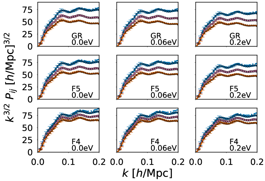
Figure 1: Real-space non-linear power spectra for various gravity models and neutrino masses at $z=1$. Points represent the results of paired-fixed MG-PICOLA N-body simulations, while lines are the result of MG-Copter. The blue circles and dashed-dotted line give the density auto-correlated power spectra $P_{\delta\delta}$, the pink squares and dashed line give the density-velocity divergence cross-correlated power spectra $P_{\delta\theta}$, while the orange triangles and solid line give the velocity divergence auto-correlated power spectra $P_{\theta\theta}$.

Figure 2 displays the same data but presented as the ratio of the full non-linear power spectra to their linear components, which helps to show where the modelling of non-linearities with MG-Copter becomes inaccurate. Figure 3 again shows the same data but presented as the ratio of the power-spectra with and without massive neutrinos for both the $0.06$eV and $0.2$eV neutrinos. The scale up to which MG-Copter closely follows the results of the MG-PICOLA simulations is marginally improved due to taking the ratio between power spectra in two models.

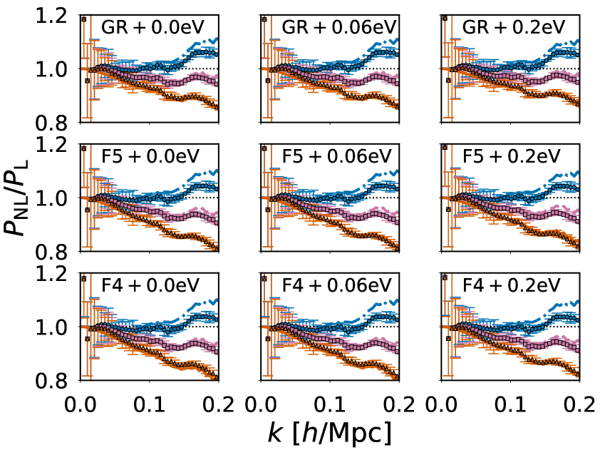
Figure 2: As in Fig. 1 but for the ratio of the real-space non-linear power spectra to their linear counterparts.

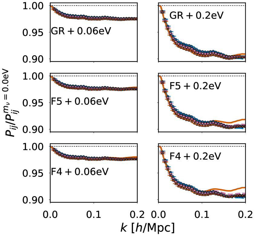
Figure 3: As in Fig. 1, but for the ratio of real-space non-linear power spectra with and without neutrino mass.

Next, we look at the comparison between MG-PICOLA and MG-Copter with $\sigma_{v}$ fitted to the MG-PICOLA simulations in the non-linear redshift-space power spectra in Figs. 4, 5 and 6. Figure 4 shows the monopole $P_{0}$ and quadrupole $P_{2}$ of the redshift-space power spectra for GR, F5, and F4 gravity models each with $0.0$eV, $0.06$eV, and $0.2$eV neutrinos. We display the results computed from paired-fixed MG-PICOLA simulations and MG-Copter with the TNS velocity dispersion parameter $\sigma_{v}$ fitted to the MG-PICOLA simulations up to $k=0.15~{}h/{\rm Mpc}$ in the form $k^{3/2}P_{i}(k)$; the figure includes the best-fitting values of $\sigma_{v}$ (expressed in RSD displacement units ${\rm Mpc}/h$) and the reduced $\chi^{2}$ for each model. The error bars on the MG-PICOLA points are taken from the inverse covariance matrices used in the $\sigma_{v}$ fitting procedure, whose computation is described at the end of Section 2.1. The $\sigma_{v}$ fitting procedure prioritises recovering the monopole $P_{0}$, and thus the agreement between MG-Copter and MG-PICOLA is slightly worse for the quadrupole $P_{2}$. As expected, for each gravity model increasing the mass of the neutrinos leads to a decrease in the best-fitting value of $\sigma_{v}$ and the quality of the fit increases, while for a fixed neutrino mass increasing the strength of the modification of gravity from GR to F5 and then F4 leads to an increase in the best-fitting value of $\sigma_{v}$ and a slightly worse quality of fit. The reason for this behaviour is that enhancement to gravity leads to an increase in the velocities of galaxies around an overdensity, thus increasing the non-linear damping, while massive neutrinos have the opposite effect due to their suppression of structure formation. The quality of the fit is better when the non-linearity is smaller and vice versa. However, in all cases the quality of the fit of MG-Copter to MG-PICOLA is good up to quasi-non-linear scales.

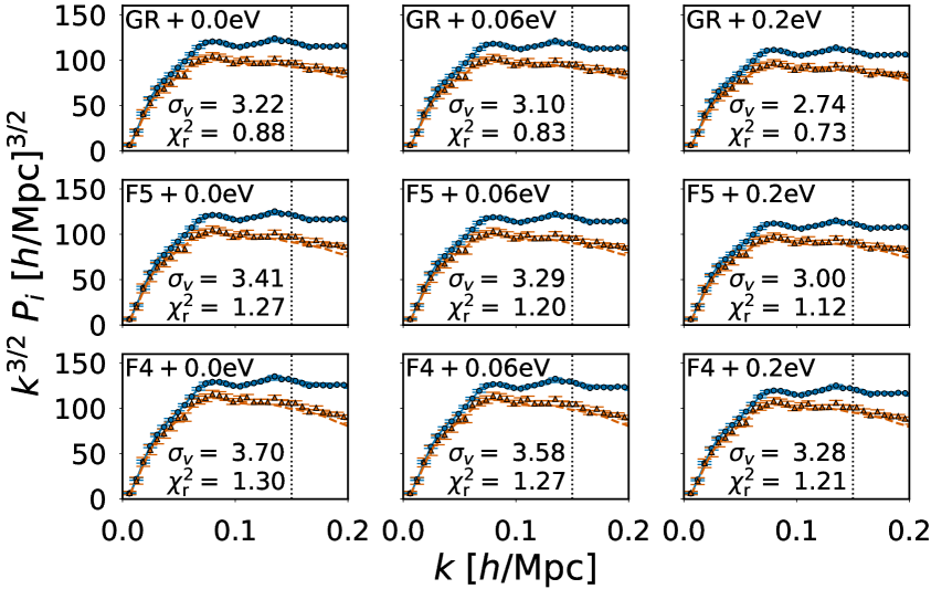
Figure 4: Redshift-space non-linear power spectra for various gravity models and neutrino masses at $z=1$. Points represent the results of paired-fixed MG-PICOLA N-body simulations, while solid lines are the result of MG-Copter with velocity dispersion $\sigma_{v}$ fitted to MG-PICOLA up to $k=0.15~{}h/{\rm Mpc}$, shown by the vertical dashed line. The error bars are those of an ideal survey with survey volume $V_{\rm s}=10~{}{\rm Gpc}^{3}/h^{3}$ and galaxy density $\bar{n}_{\rm g}=4\times 10^{-3}~{}h^{3}/{\rm Mpc}^{3}$. The blue circles and solid line give the monopole $P_{0}$, and the orange squares and dashed line give the quadrupole $P_{2}$.

Figure 5 displays the same data as Fig. 4 but presented as the ratio of the full non-linear multipoles to their linear counterparts computed with the Kaiser RSD model [42], while Fig. 6 presents the data of Fig. 4 as the ratio of the non-linear power-spectra multipoles with and without massive neutrinos for both the $0.06$eV and $0.2$eV neutrinos. The error bars on the MG-PICOLA points in these two figures represent the standard deviation of the 5 additional MG-PICOLA simulations. As in real-space, the scale up to which MG-Copter closely follows the results of the MG-PICOLA simulations is slightly improved due to taking the ratio between power spectra in two models.

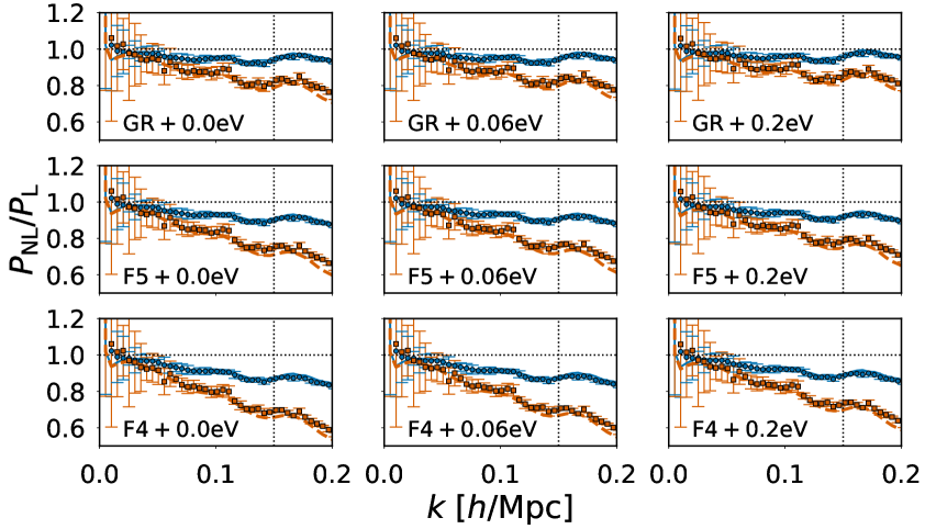
Figure 5: As in Fig. 4 but for the ratio of the redshift-space power spectrum multipoles to their linear (Kaiser) counterparts. The error bars on the MG-PICOLA points represent the standard deviation of the five additional MG-PICOLA simulations.

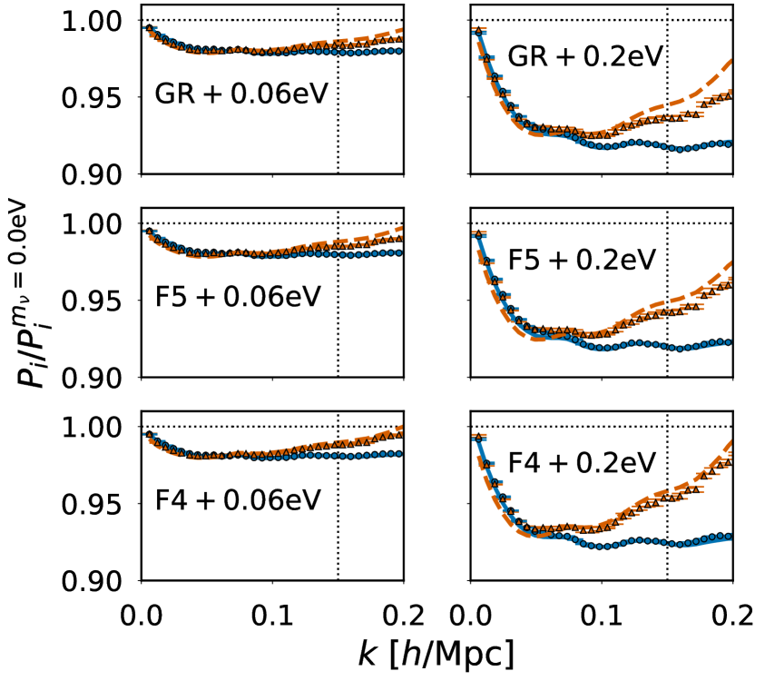
Figure 6: As in Fig. 4, but for the ratio of redshift-space non-linear power spectra with and without neutrino mass. The error bars on the MG-PICOLA points represent the standard deviation of the five additional MG-PICOLA simulations.

We also quantify the ability of MG-Copter to recover the redshift-space multipole results of MG-PICOLA through $\chi^{2}_{m_{\nu}}$; the difference between the redshift-space multipoles with and without neutrino mass. In Fig. 7 we display $\chi^{2}_{m_{\nu}}$ as a function of the maximum comparison scale $k_{\rm max}$ for GR, F5, and F4 each with $0.06$eV and $0.2$eV neutrinos at $z=1$. Here, MG-Copter is fitted to the MG-PICOLA simulations up to $k_{\rm max}$ with the covariance computed assuming an ideal survey as described at the end of Section 2.1. The agreement in $\chi^{2}_{m_{\nu}}$ between MG-PICOLA and MG-Copter fitted to MG-PICOLA is excellent in all cases. This implies that MG-Copter with $\sigma_{v}$ fitted to simulations is capable of capturing the effect of massive neutrinos accurately.

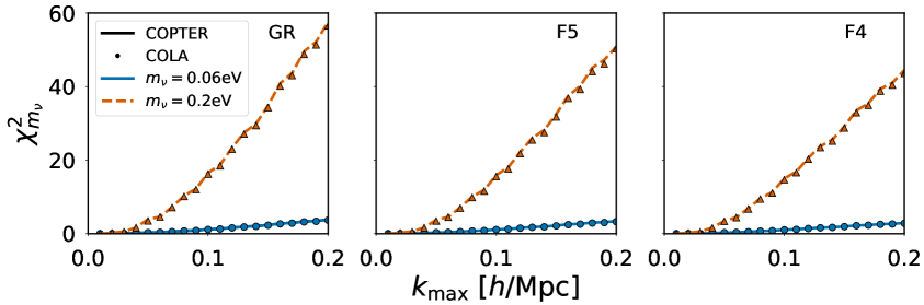
Figure 7: Difference between the redshift-space multipoles with and without neutrino mass $\chi^{2}_{m_{\nu}}$ as a function of the maximum scale $k_{\rm max}$ at $z=1$ for GR in the left panel, F5 in the middle panel, and F4 in the right panel. Points represent the results of paired-fixed MG-PICOLA N-body simulations, while solid lines are the result of MG-Copter with velocity dispersion $\sigma_{v}$ fitted to MG-PICOLA up to $k=k_{\rm max}$. Blue data corresponds to $m_{\nu}=0.06\mathrm{eV}$, and orange to $m_{\nu}=0.2\mathrm{eV}$.

4 Degeneracy

With the inclusion of modified gravity and massive neutrinos in MG-Copter the degeneracy between the two effects can be investigated.

4.1 Real- and redshift-space

We start by studying the degeneracy between modified gravity and massive neutrinos in real space.

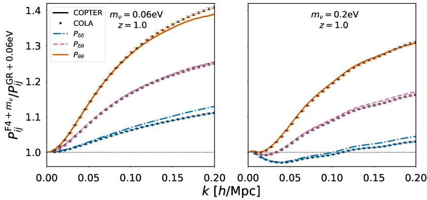
Figure 8: Ratio of real-space power spectra in F4 with $m_{\nu}=0.06$eV (left panel) and $m_{\nu}=0.2$eV (right panel) to the fiducial model of GR with $m_{\nu}=0.06$eV at $z=1$. Points represent the results of paired-fixed MG-PICOLA N-body simulations, while lines are the result of MG-Copter. The blue circles and dashed-dotted line give the density auto-correlated power spectra $P_{\delta\delta}$, the pink squares and dashed line give the density-velocity divergence cross-correlated power spectra $P_{\delta\theta}$, while the orange triangles and solid line give the velocity divergence auto-correlated power spectra $P_{\theta\theta}$.

In Fig. 8 we display the ratio of real-space power spectra in F4 gravity with $0.06$eV neutrinos in the left panel and $0.2$eV neutrinos in the right panel to a fiducial model which we take to be GR with $0.06$eV neutrinos at $z=1$. We show results for the density auto-correlation $P_{\delta\delta}$, the velocity divergence auto-correlation $P_{\theta\theta}$, and the density-velocity divergence cross-correlation $P_{\delta\theta}$. The results of paired-fixed MG-PICOLA simulations and of MG-Copter are plotted. The error bars on the MG-PICOLA results are computed using the standard deviation over the five additional simulations. In all cases, the results of MG-Copter agree well with those of MG-PICOLA up to quasi-non-linear scales around $k=0.1~{}h/{\rm Mpc}$. The left panel, where the neutrino masses are the same in both GR and F4, shows the scale-dependent enhancement of the real-space power spectra provided by F4 gravity. However, when heavier neutrinos are added to the F4 case, as in the right panel, this enhancement is opposed by the suppression effect of the massive neutrinos. Indeed, the right panel shows that $P_{\delta\delta}$ is a poor probe to distinguish between GR with $0.06$eV neutrinos and F4 with $0.2$eV neutrinos in this particular case. However, the two models remain distinguishable in $P_{\delta\theta}$ and $P_{\theta\theta}$, showing that velocity information has the potential to break the degeneracy between modified gravity and massive neutrinos. This was recently shown using the results of full N-body simulations [44]. However, neither $P_{\delta\theta}$ nor $P_{\theta\theta}$ can be measured directly by observations. Instead, it is necessary to extract the velocity information that is encoded within redshift-space distortions, and it is to this we turn our attention. We shall refer to GR with $0.06$eV neutrinos and F4 with $0.2$eV neutrinos as our two degenerate models.

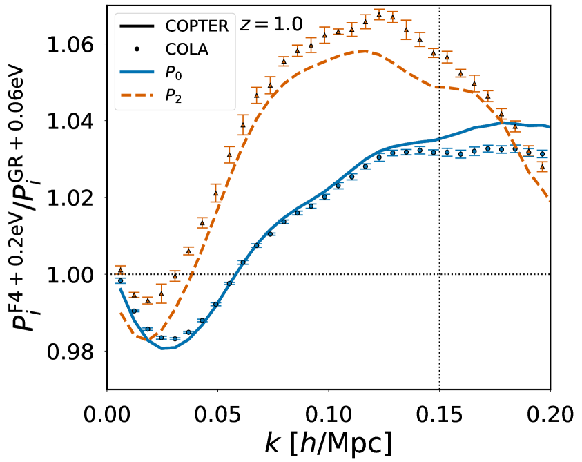
Figure 9: Degeneracy between F4 with $m_{\nu}=0.2$eV and the fiducial model of GR with $m_{\nu}=0.06$eV in the redshift-space power spectrum multipoles at $z=1$, represented as the ratio of power spectra in the two models. Points represent the results of paired-fixed MG-PICOLA N-body simulations, while solid lines are the result of MG-Copter with velocity dispersion $\sigma_{v}$ fitted to MG-PICOLA up to $k=0.15~{}h/{\rm Mpc}$. The blue circles and solid line give the monopole $P_{0}$, while the orange squares and dashed line give the quadrupole $P_{2}$. The best-fitting value of $\sigma_{v}$ for each model and the associated reduced $\chi^{2}$ are $\sigma_{v}=3.07~{}{\rm Mpc}/h$ with $\chi^{2}_{\rm r}=0.27$ for GR+$0.06$eV and $\sigma_{v}=3.23~{}{\rm Mpc}/h$ with $\chi^{2}_{\rm r}=0.39$ for F4+$0.2$eV.

In Fig. 9 we plot the redshift-space monopole and quadrupoles in F4 gravity with $0.2$eV neutrinos normalised to GR with $0.06$eV neutrinos computed with both MG-Copter and MG-PICOLA. For each model the MG-Copter result has been produced by fitting $\sigma_{v}$ to the paired-fixed MG-PICOLA simulation up to $k=0.15~{}h/{\rm Mpc}$ with the covariance computed assuming a DESI-like survey as detailed at the end of Section 2.1. The error bars on the MG-PICOLA results are computed using the standard deviation over five simulations with a boxsize of $1~{}{\rm Gpc}/h$ for each model. Firstly, this plot shows that modelling the redshift-space monopole and quadrupole using MG-Copter with $\sigma_{v}$ fitted to MG-PICOLA simulations works well. Secondly, for our degenerate models, while the monopole is still a poor probe for distinguishing between the models, the quadrupole, by virtue of the encoding of velocity information, displays differences between the two models and thus has the potential to break the degeneracy.

4.2 Redshift evolution

Our method also allows us to investigate how the degeneracy evolves with redshift in both real- and redshift-space.

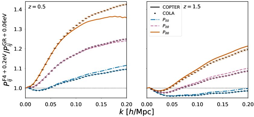
Figure 10: As in the right panel of Fig. 8, but showing the evolution of the degeneracy with redshift. The left panel corresponds to $z=0.5$ and the right to $z=1.5$.

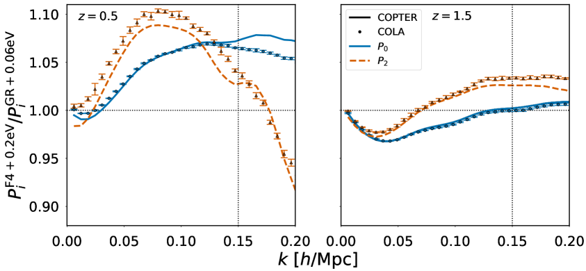
Figure 11: As in Fig. 9, but showing the evolution of the degeneracy with redshift. The left panel corresponds to $z=0.5$ and the right to $z=1.5$. For GR with $0.06$eV neutrinos, the best-fitting value of $\sigma_{v}$ and the corresponding reduced $\chi^{2}$ are $\sigma_{v}=3.84~{}{\rm Mpc}/h$ and $\chi^{2}_{\rm r}=0.29$ for $z=0.5$, and $\sigma_{v}=2.36~{}{\rm Mpc}/h$ and $\chi^{2}_{\rm r}=0.065$ for $z=1.5$. For F4 with $0.2$eV neutrinos, the best-fitting value of $\sigma_{v}$ and the corresponding reduced $\chi^{2}$ are $\sigma_{v}=4.13~{}{\rm Mpc}/h$ and $\chi^{2}_{\rm r}=0.34$ for $z=0.5$, and $\sigma_{v}=2.45~{}{\rm Mpc}/h$ and $\chi^{2}_{\rm r}=0.079$ for $z=1.5$. In all cases $\sigma_{v}$ has been fitted to MG-PICOLA up to $k=0.15~{}h/{\rm Mpc}$.

In Fig. 10 we show the real-space power spectra in the ratio between the two degenerate models as in the right panel of Fig. 8 but at $z=0.5$ (left panel) and $z=1.5$ (right panel). In Fig. 11 we show the redshift-space power spectrum multipoles in the ratio between the two degenerate models as in Fig. 9 but at $z=0.5$ (left panel) and $z=1.5$ (right panel). These figures demonstrate that the degeneracy evolves significantly with redshift, both in real- and redshift-space. Figure 10 shows that while our two degenerate models had similar matter power spectra at $z=1$ it is easier to distinguish between the two models with the matter power spectrum at other redshifts.

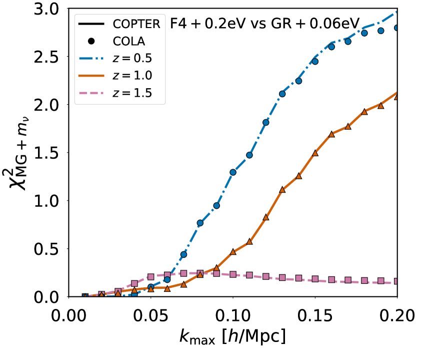
Figure 12: The redshift evolution of $\chi^{2}_{\mathrm{MG}+m_{\nu}}(k_{\rm max})$ which quantifies the difference between the redshift-space multipoles of the two degenerate models as a function of maximum comparison scale. The blue circles and dashed-dotted line correspond to $z=0.5$, the orange triangles and solid line to $z=1$, and the pink squares and dashed line to $z=1.5$. Points represent the results of paired-fixed MG-PICOLA N-body simulations, while lines are the result of MG-Copter with velocity dispersion $\sigma_{v}$ fitted to MG-PICOLA up to $k=k_{\rm max}$.

In Fig. 12 we plot the difference between the redshift-space multipoles in the two degenerate models quantified through $\chi^{2}_{\mathrm{MG}+m_{\nu}}$ as a function of the maximum comparison scale $k_{\rm max}$. We show $\chi^{2}_{\mathrm{MG}+m_{\nu}}$ as computed by both MG-PICOLA and MG-Copter with $\sigma_{v}$ fitted to MG-PICOLA up to $k_{\rm max}$ with the covariance computed assuming a DESI-like survey as detailed at the end of Section 2.1. The results from both methods agree with each other very well. We plot $\chi^{2}_{\mathrm{MG}+m_{\nu}}$ at three redshifts $z=1.5,\ 1.0,\ 0.5$ and it is clear from these results, along with those in Figs. 10 and 11, that the ability to distinguish between the redshift-space multipoles of these two models evolves with redshift. This emphasises the potential for data at multiple redshifts to break the degeneracy. The tomographic nature of weak lensing observations make them well suited to this task, and the combination of redshift-space distortion measurements with weak lensing observations could prove one of the best probes for breaking the modified gravity-massive neutrino degeneracy. However, it should be noted that systematics associated with weak lensing such as baryonic effects and intrinsic alignments may impact the effectiveness of such a probe.

5 Conclusions

In this paper, we have studied the potential for redshift-space distortions to break the degeneracy between the enhancement of structure growth provided by modifications to gravity and suppression of structure growth due to massive neutrinos, at the level of the dark matter field. For combinations of modified gravity parameters and neutrino masses that have similar matter power spectra at a given redshift, the growth rates are different and will remain distinguishable. This degeneracy-breaking growth rate information is encoded via velocities into redshift-space distortions. To carry out this work, we have modelled the effects of both modified gravity and massive neutrinos on real- and redshift-space power spectra with Standard Perturbation Theory through the code MG-Copter. We find the implementation of modified gravity and massive neutrinos in MG-Copter produces a good agreement for both real- and redshift-space power spectra with the simulation results from the code MG-PICOLA in the case of Hu-Sawicki $f(R)$ gravity.

We have then investigated the degeneracy and shown that the quadrupole of the redshift-space power spectrum retains enough of the velocity information to distinguish between GR with light neutrinos and Hu-Sawicki $f(R)$ with heavy neutrinos. The logical next step is to confirm that we can use the computationally inexpensive modelling of RSD in MG-Copter to recover a fiducial combination of $|f_{R0}|$ and $m_{\nu}$ from a simulation. An important open question for this endeavour is whether the process of fitting $\sigma_{v}$ introduces a new degeneracy, where $\sigma_{v}$ can dampen the redshift-space multipoles of a model with incorrect $|f_{R0}|$ and $m_{\nu}$ values in a way that makes them difficult to distinguish from those of the fiducial simulation. Future work will focus on extending the modelling of RSD with modified gravity and massive neutrinos to dark matter halos and galaxies in order to bring this method closer to being able to use RSD observations to jointly constrain modified gravity and massive neutrinos. It will be important to study how our conclusions change when we consider biased tracers instead of the underlying dark matter, as the bias parameters may also introduce additional degeneracies.

We have also briefly studied how the degeneracy evolves with redshift. There is a clear evolution of the degeneracy with redshift even for the matter power spectrum; for combinations of modified gravity and neutrino mass parameters that give comparable matter power spectra at one redshift, the matter power spectra at another redshift are in general likely to be distinguishable. The tomographic nature of weak lensing is particularly well suited to investigating this approach to breaking the degeneracy, although weak lensing systematics such as baryonic effects and intrinsic alignments could cause complications. Alternatively, if modified gravity is only a low redshift effect, a constraint on neutrino mass from clustering at higher redshift, for example from HI intensity mapping [66], would help break the degeneracy.

A work that appeared shortly after this paper studied RSD in halos from simulations with $f(R)$ gravity and massive neutrinos and reached conclusions broadly similar to our own [67].

References

- [1] K. Koyama, Cosmological tests of modified gravity, Reports on Progress in Physics 79 (Apr., 2016) 046902, [1504.04623].
- [2] T. Clifton, P. G. Ferreira, A. Padilla and C. Skordis, Modified gravity and cosmology, Physics Reports 513 (Mar., 2012) 1–189, [1106.2476].
- [3] G. W. Horndeski, Second-Order Scalar-Tensor Field Equations in a Four-Dimensional Space, International Journal of Theoretical Physics 10 (Sept., 1974) 363–384.
- [4] C. Deffayet, X. Gao, D. A. Steer and G. Zahariade, From k-essence to generalized Galileons, PRD 84 (Sep, 2011) 064039, [1103.3260].
- [5] T. Kobayashi, M. Yamaguchi and J. Yokoyama, Generalized G-Inflation — Inflation with the Most General Second-Order Field Equations —, Progress of Theoretical Physics 126 (Sep, 2011) 511–529, [1105.5723].
- [6] R. Laureijs, J. Amiaux, S. Arduini, J. . Auguères, J. Brinchmann, R. Cole et al., Euclid Definition Study Report, ArXiv e-prints (Oct., 2011) , [1110.3193].
- [7] DESI Collaboration, A. Aghamousa, J. Aguilar, S. Ahlen, S. Alam, L. E. Allen et al., The DESI Experiment Part I: Science,Targeting, and Survey Design, ArXiv e-prints (Oct., 2016) , [1611.00036].
- [8] D. Spergel, N. Gehrels, J. Breckinridge, M. Donahue, A. Dressler, B. S. Gaudi et al., Wide-Field InfraRed Survey Telescope-Astrophysics Focused Telescope Assets WFIRST-AFTA Final Report, ArXiv e-prints (May, 2013) , [1305.5422].
- [9] Z. Ivezic, J. A. Tyson, B. Abel, E. Acosta, R. Allsman, Y. AlSayyad et al., LSST: from Science Drivers to Reference Design and Anticipated Data Products, ArXiv e-prints (May, 2008) , [0805.2366].
- [10] L. E. H. Godfrey, H. Bignall, S. Tingay, L. Harvey-Smith, M. Kramer, S. Burke-Spolaor et al., Science at Very High Angular Resolution with the Square Kilometre Array, Publications of the ASA 29 (Jan., 2012) 42–53, [1111.6398].
- [11] A. De Felice and S. Tsujikawa, f( R) Theories, Living Reviews in Relativity 13 (June, 2010) 3, [1002.4928].
- [12] T. P. Sotiriou and V. Faraoni, f(R) theories of gravity, Reviews of Modern Physics 82 (Jan, 2010) 451–497, [0805.1726].
- [13] W. Hu and I. Sawicki, Models of f(R) cosmic acceleration that evade solar system tests, PRD 76 (Sept., 2007) 064004, [0705.1158].
- [14] Y. Fukuda, T. Hayakawa, E. Ichihara, K. Inoue, K. Ishihara, H. Ishino et al., Measurements of the Solar Neutrino Flux from Super-Kamiokande’s First 300 Days, Physical Review Letters 81 (Aug., 1998) 1158–1162, [hep-ex/9805021].
- [15] SNO Collaboration collaboration, Q. R. Ahmad, R. C. Allen, T. C. Andersen, J. D. Anglin, G. Bühler, J. C. Barton et al., Measurement of the rate of interactions produced by solar neutrinos at the sudbury neutrino observatory, Phys. Rev. Lett. 87 (Jul, 2001) 071301.
- [16] B. Pontecorvo, Mesonium and anti-mesonium, Sov. Phys. JETP 6 (1957) 429.
- [17] Particle Data Group collaboration, M. Tanabashi et al., Review of Particle Physics, Phys. Rev. D98 (2018) 030001.
- [18] J. Lesgourgues and S. Pastor, Massive neutrinos and cosmology, Physics Reports 429 (July, 2006) 307–379, [astro-ph/0603494].
- [19] J. R. Bond, G. Efstathiou and J. Silk, Massive neutrinos and the large-scale structure of the universe, Physical Review Letters 45 (Dec., 1980) 1980–1984.
- [20] E. Giusarma, M. Gerbino, O. Mena, S. Vagnozzi, S. Ho and K. Freese, Improvement of cosmological neutrino mass bounds, PRD 94 (Oct., 2016) 083522, [1605.04320].
- [21] A. J. Cuesta, V. Niro and L. Verde, Neutrino mass limits: Robust information from the power spectrum of galaxy surveys, Physics of the Dark Universe 13 (Sept., 2016) 77–86, [1511.05983].
- [22] N. Palanque-Delabrouille, C. Yèche, J. Lesgourgues, G. Rossi, A. Borde, M. Viel et al., Constraint on neutrino masses from SDSS-III/BOSS Ly forest and other cosmological probes, JCAP 2 (Feb., 2015) 045, [1410.7244].
- [23] F. Beutler, S. Saito, J. R. Brownstein, C.-H. Chuang, A. J. Cuesta, W. J. Percival et al., The clustering of galaxies in the SDSS-III Baryon Oscillation Spectroscopic Survey: signs of neutrino mass in current cosmological data sets, MNRAS 444 (Nov., 2014) 3501–3516, [1403.4599].
- [24] G.-B. Zhao, S. Saito, W. J. Percival, A. J. Ross, F. Montesano, M. Viel et al., The clustering of galaxies in the SDSS-III Baryon Oscillation Spectroscopic Survey: weighing the neutrino mass using the galaxy power spectrum of the CMASS sample, MNRAS 436 (Dec., 2013) 2038–2053, [1211.3741].
- [25] S. Vagnozzi, E. Giusarma, O. Mena, K. Freese, M. Gerbino, S. Ho et al., Unveiling secrets with cosmological data: Neutrino masses and mass hierarchy, PRD 96 (Dec, 2017) 123503, [1701.08172].
- [26] E. Giusarma, S. Vagnozzi, S. Ho, S. Ferraro, K. Freese, R. Kamen-Rubio et al., Scale-dependent galaxy bias, CMB lensing-galaxy cross-correlation, and neutrino masses, PRD 98 (Dec, 2018) 123526, [1802.08694].
- [27] A. Boyle and E. Komatsu, Deconstructing the neutrino mass constraint from galaxy redshift surveys, Journal of Cosmology and Astro-Particle Physics 2018 (Mar, 2018) 035, [1712.01857].
- [28] H. Motohashi, A. A. Starobinsky and J. Yokoyama, Cosmology Based on f(R) Gravity Admits 1 eV Sterile Neutrinos, Physical Review Letters 110 (Mar., 2013) 121302, [1203.6828].
- [29] J.-h. He, Weighing neutrinos in f(R) gravity, PRD 88 (Nov., 2013) 103523, [1307.4876].
- [30] M. Baldi, F. Villaescusa-Navarro, M. Viel, E. Puchwein, V. Springel and L. Moscardini, Cosmic degeneracies - I. Joint N-body simulations of modified gravity and massive neutrinos, MNRAS 440 (May, 2014) 75–88, [1311.2588].
- [31] B. Hu, M. Raveri, A. Silvestri and N. Frusciante, Exploring massive neutrinos in dark cosmologies with eftcamb/EFTCosmoMC, PRD 91 (Mar., 2015) 063524, [1410.5807].
- [32] H. Motohashi, A. A. Starobinsky and J. Yokoyama, Matter Power Spectrum in f(R) Gravity with Massive Neutrinos, Progress of Theoretical Physics 124 (Sept., 2010) 541–546, [1005.1171].
- [33] N. Bellomo, E. Bellini, B. Hu, R. Jimenez, C. Pena-Garay and L. Verde, Hiding neutrino mass in modified gravity cosmologies, JCAP 2 (Feb., 2017) 043, [1612.02598].
- [34] D. Alonso, E. Bellini, P. G. Ferreira and M. Zumalacárregui, Observational future of cosmological scalar-tensor theories, PRD 95 (Mar., 2017) 063502, [1610.09290].
- [35] S. Hagstotz, M. Costanzi, M. Baldi and J. Weller, Joint halo-mass function for modified gravity and massive neutrinos - I. Simulations and cosmological forecasts, MNRAS 486 (Jul, 2019) 3927–3941, [1806.07400].
- [36] DES Collaboration, T. M. C. Abbott, F. B. Abdalla, S. Avila, M. Banerji, E. Baxter et al., Dark Energy Survey Year 1 Results: Constraints on Extended Cosmological Models from Galaxy Clustering and Weak Lensing, arXiv e-prints (Oct, 2018) arXiv:1810.02499, [1810.02499].
- [37] A. Peel, V. Pettorino, C. Giocoli, J.-L. Starck and M. Baldi, Breaking degeneracies in modified gravity with higher (than 2nd) order weak-lensing statistics, A&A 619 (Nov., 2018) A38, [1805.05146].
- [38] C. Giocoli, M. Baldi and L. Moscardini, Weak lensing light-cones in modified gravity simulations with and without massive neutrinos, MNRAS 481 (Dec., 2018) 2813–2828, [1806.04681].
- [39] J. Merten, C. Giocoli, M. Baldi, M. Meneghetti, A. Peel, F. Lalande et al., On the dissection of degenerate cosmologies with machine learning, MNRAS 487 (Jul, 2019) 104–122, [1810.11027].
- [40] A. Peel, F. Lalande, J.-L. Starck, V. Pettorino, J. Merten, C. Giocoli et al., Distinguishing standard and modified gravity cosmologies with machine learning, arXiv e-prints (Oct., 2018) arXiv:1810.11030, [1810.11030].
- [41] A. J. S. Hamilton, Linear Redshift Distortions: a Review, in The Evolving Universe (D. Hamilton, ed.), vol. 231 of Astrophysics and Space Science Library, p. 185, Jan, 1998. astro-ph/9708102. DOI.
- [42] N. Kaiser, Clustering in real space and in redshift space, MNRAS 227 (July, 1987) 1–21.
- [43] J. C. Jackson, A critique of Rees’s theory of primordial gravitational radiation, MNRAS 156 (Jan, 1972) 1P, [0810.3908].
- [44] S. Hagstotz, M. Gronke, D. Mota and M. Baldi, Breaking cosmic degeneracies: Disentangling neutrinos and modified gravity with kinematic information, arXiv e-prints (Feb., 2019) arXiv:1902.01868, [1902.01868].
- [45] J. Carlson, M. White and N. Padmanabhan, Critical look at cosmological perturbation theory techniques, PRD 80 (Aug., 2009) 043531, [0905.0479].
- [46] B. Bose and K. Koyama, A perturbative approach to the redshift space power spectrum: beyond the Standard Model, JCAP 8 (Aug., 2016) 032, [1606.02520].
- [47] A. Taruya, Constructing perturbation theory kernels for large-scale structure in generalized cosmologies, PRD 94 (July, 2016) 023504, [1606.02168].
- [48] S. Tassev, M. Zaldarriaga and D. J. Eisenstein, Solving large scale structure in ten easy steps with COLA, JCAP 6 (June, 2013) 036, [1301.0322].
- [49] A. Taruya, T. Nishimichi and S. Saito, Baryon acoustic oscillations in 2D: Modeling redshift-space power spectrum from perturbation theory, PRD 82 (Sept., 2010) 063522, [1006.0699].
- [50] A. Font-Ribera, P. McDonald, N. Mostek, B. A. Reid, H.-J. Seo and A. Slosar, DESI and other Dark Energy experiments in the era of neutrino mass measurements, Journal of Cosmology and Astro-Particle Physics 2014 (May, 2014) 023, [1308.4164].
- [51] A. Upadhye, R. Biswas, A. Pope, K. Heitmann, S. Habib, H. Finkel et al., Large-Scale Structure Formation with Massive Neutrinos and Dynamical Dark Energy, Phys. Rev. D89 (2014) 103515, [1309.5872].
- [52] S. Saito, M. Takada and A. Taruya, Impact of massive neutrinos on nonlinear matter power spectrum, Phys. Rev. Lett. 100 (2008) 191301, [0801.0607].
- [53] S. Saito, M. Takada and A. Taruya, Nonlinear power spectrum in the presence of massive neutrinos: perturbation theory approach, galaxy bias and parameter forecasts, Phys. Rev. D80 (2009) 083528, [0907.2922].
- [54] A. Lewis, A. Challinor and A. Lasenby, Efficient Computation of Cosmic Microwave Background Anisotropies in Closed Friedmann-Robertson-Walker Models, ApJ 538 (Aug., 2000) 473–476, [astro-ph/9911177].
- [55] G.-B. Zhao, L. Pogosian, A. Silvestri and J. Zylberberg, Searching for modified growth patterns with tomographic surveys, PRD 79 (Apr., 2009) 083513, [0809.3791].
- [56] A. Hojjati, L. Pogosian and G.-B. Zhao, Testing gravity with CAMB and CosmoMC, JCAP 8 (Aug., 2011) 005, [1106.4543].
- [57] X. Qian and P. Vogel, Neutrino mass hierarchy, Progress in Particle and Nuclear Physics 83 (Jul, 2015) 1–30, [1505.01891].
- [58] F. Villaescusa-Navarro, A. Banerjee, N. Dalal, E. Castorina, R. Scoccimarro, R. Angulo et al., The imprint of neutrinos on clustering in redshift-space, Astrophys. J. 861 (2018) 53, [1708.01154].
- [59] C. Howlett, M. Manera and W. J. Percival, L-PICOLA: A parallel code for fast dark matter simulation, Astronomy and Computing 12 (Sep, 2015) 109–126, [1506.03737].
- [60] H. A. Winther, K. Koyama, M. Manera, B. S. Wright and G.-B. Zhao, COLA with scale-dependent growth: applications to screened modified gravity models, JCAP 8 (Aug., 2017) 006, [1703.00879].
- [61] B. S. Wright, H. A. Winther and K. Koyama, COLA with massive neutrinos, Journal of Cosmology and Astro-Particle Physics 2017 (Oct., 2017) 054, [1705.08165].
- [62] R. E. Angulo and A. Pontzen, Cosmological N-body simulations with suppressed variance, MNRAS 462 (Oct., 2016) L1–L5, [1603.05253].
- [63] F. Villaescusa-Navarro, S. Naess, S. Genel, A. Pontzen, B. Wandelt, L. Anderson et al., Statistical Properties of Paired Fixed Fields, ApJ 867 (Nov., 2018) 137, [1806.01871].
- [64] M. C. Cautun and R. van de Weygaert, The DTFE public software - The Delaunay Tessellation Field Estimator code, arXiv e-prints (May, 2011) arXiv:1105.0370, [1105.0370].
- [65] A. Zucca, L. Pogosian, A. Silvestri and G.-B. Zhao, MGCAMB with massive neutrinos and dynamical dark energy, JCAP 1905 (2019) 001, [1901.05956].
- [66] F. Villaescusa-Navarro, P. Bull and M. Viel, Weighing Neutrinos with Cosmic Neutral Hydrogen, ApJ 814 (Dec, 2015) 146, [1507.05102].
- [67] J. E. García-Farieta, F. Marulli, A. Veropalumbo, L. Moscardini, R. Casas, C. Giocoli et al., Clustering and redshift-space distortions in modified gravity models with massive neutrinos, arXiv e-prints (Feb, 2019) arXiv:1903.00154, [1903.00154].