Theory for the single-particle dynamics in glassy mixtures with particle size swaps

Abstract

We present a theory for the single-particle dynamics in binary mixtures with particle size swaps. The general structure of the theory follows that of the theory for the collective dynamics in binary mixtures with particle size swaps, which we developed previously [G. Szamel, Phys. Rev. E 98, 050601(R) (2018)]. Particle size swaps open up an additional relaxation channel, which speeds up both the collective dynamics and the single-particle dynamics. To make explicit predictions, we resort to a factorization approximation similar to that employed in the mode-coupling theory of glassy dynamics. We show that, like in the standard mode-coupling theory, the single-particle motion becomes arrested at the dynamic glass transition predicted by the theory for the collective dynamics. We compare the non-ergodicity parameters predicted by our mode-coupling-like approach for the an equimolar binary hard sphere mixture with particle size swaps with the non-ergodicity parameters predicted by the standard mode-coupling theory for the same system without swaps. Our theory predicts that the “cage size” is bigger in the system with particle size swaps.

1 Introduction

Computer simulations are an essential tool in the quest for the understanding of glassy dynamics and the glass transition [1]. Their usefulness comes from the fact that they can access particles’ positions and thus are able to provide much more detailed picture of the dynamics than even most ingenious experiments. However, for many years computer simulations had to cope with the “glass ceiling” [2]: since timescales accessible in simulations are orders of magnitude shorter than experimental timescales, computer simulations utilizing well equilibrated systems were only feasible in the temperature/density region where the dynamics are only 4-5 decades slower than in normal stable liquids.

Recently, a creative extension of the particle size swaps Monte Carlo, that was first used in the context of glassy systems’ simulations almost 30 years ago [3], was introduced. We should recall that since the original study of Ref. [3], the particle size swaps Monte Carlo method has been tried a few times [4], but with very limited success. Then, Berthier and collaborators [5, 6] turned the problem on its head by introducing several new glassy systems for which the particle size swaps Monte Carlo method speeds up the equilibration by many orders of magnitude. It is now possible to equilibrate glassy systems at temperatures comparable to and even lower than the laboratory glass transition temperature. This allowed for the investigation of static properties of glassy systems at realistic conditions [2, 7, 8, 9].

The success of the particle size swaps method opened two sets of theoretical questions: questions about the method itself and questions about our fundamental understanding of the glass transition. The latter questions are concerned with the explanation of the success of the particle size swaps method. While it is intuitively plausible that particle size swaps open a new relaxation channel and thus should speeding up the dynamics, the amount of the speed-up is quite significant and calls for a more detailed explanation. Additionally, one would like to understand theoretically when does the particle size swaps method work and when it does not. Finally, one would like to describe the eventual slowing down of the particle size swaps Monte Carlo method and compare it with the slowing down of local dynamics, either Monte Carlo, or Brownian, or Newtonian dynamics.

Out of the second set of questions opened by the success of the particle size swaps Monte Carlo, probably the most crucial one is concerned with the importance of cooperative processes operating on length scales that increase upon approaching the glass transition compared to the importance of local dynamics’ slowing down [10, 11]. Additional questions are concerned with the relevance of configurational entropies calculated theoretically by introducing order parameters that explicitly forbid or allow particle size swaps [12, 13].

In spite of these interesting questions raised by the success of the particle size swaps Monte Carlo method, the theoretical analysis of this method is in its infancy. Three approaches have been proposed. First, Ikeda et al. [12, 13] proposed to use the close relationship between the dynamics of mean-field models and the replica theory-based description of these models. Specifically, they used the correspondence between the dynamic transition predicted by the dynamic (mode-coupling-like) theory and identified with the dynamic crossover observed in simulations and the dynamic transition predicted by the replica approach. They argued that in the presence of particles size swaps one has to adopt a more general structure of the ansatz for the inter-replica correlation functions, which are the order parameters within the replica approach. They showed that the new ansatz leads to a shift of the dynamic transition towards larger volume fractions, in qualitative agreement with the simulations.

Next, Brito et al. [14], in the context of continuous distribution of particles’ diameters, proposed to treat the diameters as additional variables, endowed with their own equations of motion (stochastic in the case of the Monte Carlo dynamics and deterministic continuous time equations in the case of the Newtonian-like dynamics). This allowed Brito et al. to put forward some general arguments, which imply that allowing particle size swaps should lead to the decrease of the onset temperature for the glassy dynamics. However, their arguments do not lead to any quantitative prediction for this change nor to any prediction for the actual dynamical behavior with particle size swaps. Nevertheless, Brito et al.’s idea of treating particles’ diameters as additional variables is extremely useful and it has already lead to generalizations of the original particle size swaps Monte Carlo method [15, 16].

We developed a dynamic theory for the acceleration due to the particle size swaps [17]. The general structure of our theory agrees with the physical intuition: particle size swaps act as an additional relaxation channel, which speeds up the dynamics. To make explicit predictions we had to approximate the so-called irreducible memory functions, which are the main unknown theoretical quantities in our approach. To this end we used a factorization approximation of the type utilized in the mode-coupling theory of glassy dynamics and the glass transition [18]. We calculated an approximate glass transition phase diagram for an equimolar binary hard-sphere mixture. The presence of particle size swaps shifts the dynamic glass transition towards higher volume fractions. The shift increases with increasing ratio of the hard-sphere diameters; it saturates at about 4% at the diameter ratio of approximately 1.2. We would like to emphasize that in our theory the set of order parameters does not depend on whether particle size swaps are allowed or not. It is the set of self-consistent equations for the order parameters that changes. This is in contrast with the approach of Ikeda et al.

Here we extend the previously presented theory to the case of single-particle motion. This extension will allow us to study the frozen-in part of the self-van Hove function (albeit in the reciprocal space) and compare the localization lengths with and without particle size swaps. Notably, the set of order parameters for the single-particle motion does depend on whether particle size swaps are allowed or not. This is due to the fact that without particle size swaps there cannot be any single-particle cross-correlations.

Generally speaking, the relation of the structure of the theory for the single-particle motion and the previously derived theory for the collective dynamics is very similar to the relation between the same theories within the standard mode-coupling theory of the glass transition. In particular, in the present case involving particle size swaps and in the standard theory describing local dynamics, single-particle motion becomes arrested at the dynamic glass transition predicted by the theory for collective dynamics.

The paper is organized as follows. In the next section we discuss the model system with particle size swaps that we analyze and introduce the self-intermediate scattering functions that quantify the single-particle dynamics. In Sec. 3 we express these functions in terms of the so-called memory functions. In Sec. 4 we introduce the main approximation of the theory, the factorization approximation, and use it to express the memory functions in terms of the intermediate scattering functions. In Sec. 5 we present numerical results for the non-decaying parts of the intermediate scattering functions in the glassy phase predicted by the theory. We end with some discussion in Sec. 6.

2 Model: Binary mixture with particle size swaps

We consider the model investigated in Ref. [17], i.e. a binary mixture. This is the simplest model that allows one to investigate the influence of the particle size swaps on the dynamics. Two arguments can be made against using a binary mixture. First, computer simulations studies [6] showed that particle size exchanges in systems with a continuous polydispersity result in the largest speed-up of the dynamics. Second, a system with a continuous polydispersity allows one to treat the particles’ diameters as additional variables that evolve according to their own equation of motion [14]. The distribution of the particles diameters is then enforced by a diameter-dependent chemical potential-like term, which plays the role of an one-particle external potential for the diameter variable. The evolution of particles positions and sizes could then be implemented in a very similar way. However, the price that one has to pay for this uniformity of the evolution equations is that one has to deal with a static problem with infinitely many components. This makes explicit calculations a bit daunting.

To investigate the single-particle dynamics we consider a binary mixture consisting of $N$ particles in volume $V$. We assume that one of these particles, for convenience the particle number 1, is tagged and focus our attention on the motion of this particle. All the particles, including the tagged particle, can be of type $A$ or $B$. These particles types differ by size. Since any particle can change its type, the state of particle $i$ is determined by its position, $\mathbf{r}_{i}$, and type indicated by a binary variable $\sigma_{i}$, with $\sigma_{i}=1$ corresponding to $A$ and $\sigma_{i}=-1$ corresponding to $B$. The composition of the system is specified by the difference of the chemical potentials of particles of type $A$ and $B$, $\Delta\mu$. We note that for a given chemical potential difference, the composition depends also on the number density $n=N/V$ and the temperature $T$ of the system. We will assume that these three parameters result in concentrations $x_{A}$ and $x_{B}=1-x_{A}$, and that these concentration are constant while the density or the temperature of the system varies. We note that this implies that the tagged particle can be of type $A$ with probability $x_{A}$ and of type $B$ with probability $x_{B}$. In practical calculations we will restrict ourselves to equimolar mixtures (for which some formulas simplify). We assume that the “normal” dynamics of the system is Brownian, i.e., that each particle moves under the combined influence of thermal noise and interparticle forces. The forces are derived from a spherically symmetric potential, which depends on the particle type, $V_{\sigma_{i}\sigma_{j}}(r_{ij})$, where $r_{ij}=|\mathbf{r}_{i}-\mathbf{r}_{j}|$ is the distance between particles $i$ and $j$. In addition to the Brownian motion in space, the particles can change their type (size). We assume that each particle can change its type independently of the type changes of other particles. This is analogous to the single-spin-flip dynamics of spin systems. In contrast, in the initial computational studies [5, 6] particle size swaps were done in such a way that the number of particles of each size was conserved. This procedure is analogous to the so-called Kawasaki dynamics of spin systems. It is convenient in simulational studies because it allows one to maintain easily a specific composition of the system. Later investigations [15, 16] showed that replacing the Kawasaki-type procedure by single particle size swaps is a relatively mild change and that both procedures lead to very similar results.

The above described model corresponds to the following equation of motion for the $N$-particle distribution, $P_{N}(\mathbf{r}_{1},\sigma_{1},...,\mathbf{r}_{N},\sigma_{N};t)$, abbreviated below as $P_{N}$,

$$\partial_{t}P_{N}=\Omega_{\text{sw}}P_{N}\equiv\left(\Omega+\delta\Omega_{\text{sw}}\right)P_{N}.$$ (1)

Here the evolution operator $\Omega_{\text{sw}}$ consists of two parts describing two relaxation channels, the part describing Brownian motion of particles,

$$\Omega=D_{0}\sum_{i}\partial_{\mathbf{r}_{i}}\cdot\left(\partial_{\mathbf{r}_{i}}-\beta\mathbf{F}_{i}\right)$$ (2)

and the part describing particle size swaps,

$$\delta\Omega_{\text{sw}}=-\tau_{\text{sw}}^{-1}\sum_{i}\left(1-S_{i}\right)w_{i}.$$ (3)

In Eq. (2) $D_{0}$ is the diffusion coefficient of an isolated particle, $D_{0}=k_{B}T/\xi_{0}$, with $\xi_{0}$ being the friction coefficient of an isolated particle, $\beta=1/k_{B}T$, and $\mathbf{F}_{i}$ is the total force on particle $i$, $\mathbf{F}_{i}=\sum_{j\neq i}\mathbf{F}_{ij}=-\sum_{j\neq i}\partial_{\mathbf{r}_{i}}V_{\sigma_{i}\sigma_{j}}(r_{ij})$. In Eq. (3) $\tau_{\text{sw}}$ is the rate of attempted particle size swaps, $S_{i}$ is the swap operator, $S_{i}\sigma_{i}=-\sigma_{i}$, and $w_{i}$ is the factor ensuring that the detailed balance condition, $\left(1-S_{i}\right)w_{i}P_{N}^{eq}=0$, is satisfied, with $P_{N}^{eq}$ being the equilibrium distribution, $P_{N}^{eq}\propto\exp\left(-\beta\sum_{i\neq j}V_{\sigma_{i}\sigma_{j}}(r_{ij})+\sum_{i}\frac{\beta}{2}\Delta\mu\sigma_{i}\right)$. The factor $w_{i}$ depends on the way particle size swaps are attempted. In practical applications one typically uses Metropolis criterion for accepting attempted swaps. It should be emphasized that while the interactions influencing particles’ motion in space are pairwise-additive, the factor $w_{i}$ typically is not and it depends on the whole neighborhood of particle $i$.

The focus of the present investigation are the elements of the matrix of the self-intermediate correlation functions, i.e. the single-particle (tagged particle) density correlation functions,

$$F_{\alpha\beta}^{s}(q;t)=\left<n_{\alpha}^{s}(\mathbf{q})e^{\Omega_{\text{sw}}t}n_{\beta}^{s}(-\mathbf{q})\right>,$$ (4)

where $n_{\alpha}^{s}$ is the Fourier transform of the microscopic tagged particle density,

$$n_{\alpha}^{s}(\mathbf{q})=\frac{1+\sigma_{1}\left(\delta_{\alpha A}-\delta_{\alpha B}\right)}{2}e^{-i\mathbf{q}\cdot\mathbf{r}_{1}}.$$ (5)

To develop a theory for the dynamics of $F_{\alpha\beta}^{s}(q;t)$ we will also need the collective density correlation functions,

$$F_{\alpha\beta}(q;t)=\left<n_{\alpha}(\mathbf{q})e^{\Omega_{\text{sw}}t}n_{\beta}(-\mathbf{q})\right>,$$ (6)

where $n_{\alpha}$, $\alpha=A,B$, are the Fourier transforms of the normalized microscopic densities of particles of type $\alpha$,

$$n_{\alpha}(\mathbf{q})=\frac{1}{\sqrt{N}}\sum_{i>1}\frac{1+\sigma_{i}\left(\delta_{\alpha A}-\delta_{\alpha B}\right)}{2}e^{-i\mathbf{q}\cdot\mathbf{r}_{i}}.$$ (7)

In Eqs. (4,6) and in the following equations the standard conventions apply: $\left<\dots\right>$ denotes the semi-grand canonical ensemble average over $P_{N}^{eq}$, the equilibrium probability distribution stands to the right of the quantity being averaged, and all operators act on it as well as on everything else.

We should emphasize the contrast between the single-particle and collective density correlation functions. In the absence of particle size swaps the matrix of the self-intermediate correlation functions is diagonal and the following notation is used $F_{\alpha}^{s}(q;t)\equiv F_{\alpha\alpha}^{s}(q;t)$, $\alpha=A,B$. In the presence of particle size swaps the tagged particle can change its type, which leads to the appearance of the off-diagonal terms in the matrix of the self-intermediate correlation functions. In contrast, the set of collective density correlation functions is the same regardless of the presence of particle size swaps.

In the approach of Ikeda et al., the order parameters are the replica theory analogues of the single-particle density correlations (physically, the long-time limits of the time-dependent single-particle density correlation functions should be equal to the replica theory single-particle correlations; note that a truly consistent dynamic and static description of the glass transition is still lacking, except in infinite spatial dimension). Thus, one could argue that it is natural that in that approach a different set of order parameters is used depending on the presence of particle size swaps.

3 Memory function representation

To derive the memory function representation of the tagged particle density correlations we use the standard projection operator procedure [19]. First, we define a projection operator on the tagged particle density subspace, $\mathcal{P}^{s}$,

$$\mathcal{P}^{s}=\dots\sum_{\alpha}\left.n_{\alpha}^{s}(-\mathbf{k})\right>x_{\alpha}^{-1}\left<n_{\alpha}^{s}(\mathbf{k})\right.\dots.$$ (8)

and the orthogonal projection, $\mathcal{Q}$,

$$\mathcal{Q}^{s}=\mathcal{I}-\mathcal{P}^{s}\equiv\mathcal{I}-\dots\sum_{\alpha}\left.n_{\alpha}^{s}(-\mathbf{k})\right>x_{\alpha}^{-1}\left<n_{\alpha}^{s}(\mathbf{k})\right.\dots.$$ (9)

Note that $\left<n_{\alpha}^{s}(\mathbf{k})n_{\beta}^{s}(-\mathbf{k})\right>\equiv F_{\alpha\beta}^{s}(\mathbf{k};t=0)=x_{\alpha}\delta_{\alpha\beta}$.

Next, we use the standard projection operator identity [18]

$$\frac{1}{z-\Omega_{\text{sw}}}=\frac{1}{z-\Omega_{\text{sw}}\mathcal{Q}}+\frac{1}{z-\Omega_{\text{sw}}\mathcal{Q}}\Omega_{\text{sw}}\mathcal{P}\frac{1}{z-\Omega_{\text{sw}}}.$$ (10)

to express the Laplace transform of the time derivative of the tagged particle density correlation function, $zF_{\alpha\beta}^{s}(q;z)-F_{\alpha\beta}^{s}(q;t=0)$, in terms of the tagged particle reducible memory function,

$$zF_{\alpha\beta}^{s}(q;z)-F_{\alpha\beta}^{s}(q;t=0)=\left<n_{\alpha}^{s}(\mathbf{q})\Omega_{\text{sw}}\frac{1}{z-\Omega_{\text{sw}}}n_{\beta}^{s}(-\mathbf{q})\right>$$

$$= \left<n_{\alpha}^{s}(\mathbf{q})\Omega_{\text{sw}}\left(\mathcal{P}^{s}+\mathcal{Q}^{s}\right)\frac{1}{z-\Omega_{sw}}n_{\beta}^{s}(-\mathbf{q})\right>$$

$$= \sum_{\gamma}\left<n_{\alpha}^{s}(\mathbf{q})\Omega_{\text{sw}}n_{\gamma}^{s}(-\mathbf{q})\right>x_{\gamma}^{-1}\left<n_{\gamma}^{s}(\mathbf{q})\frac{1}{z-\Omega_{\text{sw}}}n_{\beta}^{s}(-\mathbf{q})\right>$$

$$+\sum_{\gamma}\left<n_{\alpha}^{s}(\mathbf{q})\Omega_{\text{sw}}\mathcal{Q}^{s}\frac{1}{z-\Omega_{\text{sw}}\mathcal{Q}^{s}}\mathcal{Q}^{s}\Omega_{\text{sw}}n_{\gamma}^{s}(-\mathbf{q})\right>x_{\gamma}^{-1}\left<n_{\gamma}^{s}(\mathbf{q})\frac{1}{z-\Omega_{\text{sw}}}n_{\beta}^{s}(-\mathbf{q})\right>.$$

In the second line of Eq. (3) we identify the tagged particle frequency matrix,

$$O_{\alpha\beta}^{s}(q) = -\left<n_{\alpha}^{s}(\mathbf{q})\Omega_{\text{sw}}n_{\beta}^{s}(-\mathbf{q})\right>=D_{0}\mathbf{q}^{2}x_{\alpha}\delta_{\alpha\beta}+\tau_{\text{sw}}^{-1}\left<n_{\alpha}^{s}(\mathbf{q})\left(1-S_{1}\right)w_{1}n_{\beta}^{s}(-\mathbf{q})\right>$$ (12)

$$= D_{0}\mathbf{q}^{2}x_{\alpha}\delta_{\alpha\beta}+\frac{1}{2\tau_{\text{sw}}}\left<w_{1}\right>\left(2\delta_{\alpha\beta}-1\right),$$

and in the third line we identify the matrix of the tagged particle reducible memory functions,

$$M_{\alpha\beta}^{s\text{red}}(q;z) = \left<n_{\alpha}^{s}(\mathbf{q})\Omega_{\text{sw}}\mathcal{Q}^{s}\left(z-\mathcal{Q}^{s}\Omega_{\text{sw}}\mathcal{Q}^{s}\right)^{-1}\mathcal{Q}^{s}\Omega_{\text{sw}}n_{\beta}^{s}(-\mathbf{q})\right>.$$ (13)

We note that, like in the collective dynamics problem [17], the tagged particle frequency matrix can be decomposed into the part corresponding to “normal” (i.e. Brownian) and the part describing particle size swaps. This separation can be conveniently expressed by introducing 3-dimensional vectors $\mathsf{v}_{\alpha}$, $\alpha=A,B$, and a 3x3 matrix $\mathsf{O}^{s}$,

$$O_{\alpha\beta}^{s}(q) = \mathsf{v}_{\alpha}^{\text{T}}\mathsf{O}^{s}(q)\mathsf{v}_{\beta}$$ (14)

Here $\mathsf{v}_{A}^{\text{T}}=(1,0,1)$, $\mathsf{v}_{B}^{\text{T}}=(0,1,-1)$, $\mathsf{O}_{11}^{s}=D_{0}q^{2}x_{A}$, $\mathsf{O}_{22}^{s}=D_{0}q^{2}x_{B}$, $\mathsf{O}_{33}^{s}=(1/2\tau_{\text{sw}})\left<w_{1}\right>$ and $\mathsf{O}_{ab}=0$ for $a\neq b$. Thus, Brownian dynamics is represented by elements of matrix $\mathsf{O}^{s}$ with $a,b\leq 2$ and the particle size swaps are represented by the 33 element of $\mathsf{O}^{s}$.

Next, we note the structure of the “vertexes” in the matrix of the tagged particle reducible memory functions,

$$\left.\mathcal{Q}^{s}\Omega_{\text{sw}}n_{\alpha}^{s}(-\mathbf{q})\right> = \left.D_{0}\mathcal{Q}^{s}i\mathbf{q}\cdot\left(i\mathbf{q}+\beta\mathbf{F}_{1}\right)\frac{1+\sigma_{1}\left(\delta_{\alpha A}-\delta_{\alpha B}\right)}{2}e^{i\mathbf{q}\cdot\mathbf{r}_{1}}\right>$$ (15)

$$-\left.\frac{1}{\tau_{\text{sw}}}\mathcal{Q}^{s}w_{1}\sigma_{1}e^{i\mathbf{q}\cdot\mathbf{r}_{1}}\right>\left(\delta_{\alpha A}-\delta_{\alpha B}\right)$$

$$= \sum_{a}\left.\pi_{a}^{s}(-\mathbf{q})\right>\mathsf{v}_{\alpha a},$$

where functions $\pi_{a}^{s}$ are defined as follows,

$$\pi_{1,2}^{s}(\mathbf{q})\!\! = \!\!D_{0}\mathcal{Q}^{s}i\mathbf{q}\cdot\left(i\mathbf{q}-\beta\mathbf{F}_{1}\right)\frac{1\pm\sigma_{1}}{2}e^{-i\mathbf{q}\cdot\mathbf{r}_{1}},$$ (16)

$$\pi_{3}^{s}(\mathbf{q})\!\! = \!\!-\frac{1}{\tau_{\text{sw}}}\mathcal{Q}^{s}w_{1}\sigma_{1}e^{-i\mathbf{q}\cdot\mathbf{r}_{1}}.$$ (17)

and $\mathsf{v}_{\alpha a}$ is the $a$th element of vector $\mathsf{v}_{\alpha}$.

The structure of the vertexes uncovered in Eq. (15) allows us to express the matrix of the tagged particle reducible memory functions $M^{s\text{red}}$ in terms of 3-dimensional vectors $\mathsf{v}_{\alpha}$, $\alpha=A,B$, and a 3x3 matrix $\mathsf{M}^{s\text{red}}$,

$$M_{\alpha\beta}^{s\text{red}}(q;z) = \mathsf{v}_{\alpha}^{\text{T}}\mathsf{M}^{s\text{red}}(q;z)\mathsf{v}_{\beta},$$ (18)

where the matrix elements of $\mathsf{M}^{s\text{red}}$ read

$$\mathsf{M}_{ab}^{s\text{red}}(q;z)=\left<\pi_{a}^{s}(\mathbf{q})\left(z-\mathcal{Q}^{s}\Omega_{\text{sw}}\mathcal{Q}^{s}\right)^{-1}\pi_{b}^{s}(-\mathbf{q})\right>.$$ (19)

Again, this representation allows us to separate “normal” (i.e. Brownian) dynamics represented by elements of matrix $\mathsf{M}^{s\text{red}}$ with $a,b\leq 2$ and the particle swaps represented by the 33 element of $\mathsf{M}^{s\text{red}}$. We note, however, that while matrix $\mathsf{O}^{s}$ is diagonal, in general, matrix $\mathsf{M}^{s\text{red}}$ is not. Thus, in general, there will be terms describing the time-delayed couplings between the two relaxation channels. These couplings are described by elements $\mathsf{M}^{s\text{red}}$ with $a\leq 2$ and $b=3$, and $a=3$ and $b\leq 2$.

Finally, we introduce the tagged particle irreducible evolution operator. This will allow us to introduce a 3x3 matrix $\mathsf{M}^{s\text{irr}}$, whose elements are functions evolving with the so-called irreducible evolution operator. For systems evolving with Brownian dynamics this step was introduced and justified by Cichocki and Hess [20]. Later, Kawasaki [21] argued that an analogous construction should also be applied for a more general class of systems evolving with stochastic dynamics, including spin systems evolving with spin-flip dynamics. We recall that our dynamics is a combination of Brownian dynamics and particle size swaps, and the latter events are technically implemented in terms of single spin flips.

We follow the definition of the collective dynamics irreducible evolution operator [17] and define the tagged particle irreducible evolution operator as follows,

$$\Omega_{\text{sw}}^{s\text{irr}} = \mathcal{Q}^{s}\Omega_{\text{sw}}\mathcal{Q}^{s}-\sum_{\alpha\beta}\left.\mathcal{Q}^{s}\Omega n_{\alpha}^{s}(-\mathbf{q})\right>\left<n_{\alpha}^{s}(\mathbf{q})\Omega n_{\beta}^{s}(-\mathbf{q})\right>^{-1}\left<n_{\beta}^{s}(\mathbf{q})\Omega\mathcal{Q}^{s}\right.$$ (20)

$$-\left.\mathcal{Q}^{s}\delta\Omega_{\text{sw}}\sigma^{s}(-\mathbf{q})\right>\left<\sigma^{s}(\mathbf{q})\delta\Omega_{\text{sw}}\sigma^{s}(-\mathbf{q})\right>^{-1}\left<\sigma^{s}(\mathbf{q})\delta\Omega_{\text{sw}}\mathcal{Q}^{s}\right.,$$

where $\sigma^{s}(\mathbf{q})=\sigma_{1}e^{-i\mathbf{q}\cdot\mathbf{r}_{1}}$. With the help of matrix $\mathsf{O}^{s}$ Eq. (20) can be re-written as

$$\Omega_{\text{sw}}^{s\text{irr}} = \mathcal{Q}^{s}\Omega_{\text{sw}}\mathcal{Q}^{s}+\sum_{a,b}^{2}\left.\pi_{a}^{s}(-\mathbf{q})\right>\left(\mathsf{O}^{s}\right)^{-1}_{ab}\left<\pi_{b}^{s}(\mathbf{q})\right.+\left.2\pi_{3}^{s}(-\mathbf{q})\right>\left(4\mathsf{O}^{s}\right)^{-1}_{33}\left<2\pi_{3}^{s}(\mathbf{q})\right.$$ (21)

$$= \mathcal{Q}^{s}\Omega_{\text{sw}}\mathcal{Q}^{s}+\sum_{a,b}\left.\pi_{a}^{s}(-\mathbf{q})\right>\left(\mathsf{O}^{s}\right)^{-1}_{ab}(q)\left<\pi_{b}^{s}(\mathbf{q})\right..$$

We note that, like in the case of the collective dynamics irreducible operator, one-particle reducible parts of $\mathcal{Q}^{s}\Omega_{\text{sw}}\mathcal{Q}^{s}$ are removed separately for Brownian dynamics and particle size swaps.

Next, we use a formula analogous to Eq. (10),

$$\frac{1}{z-\mathcal{Q}^{s}\Omega_{\text{sw}}\mathcal{Q}^{s}} = \frac{1}{z-\Omega_{\text{sw}}^{s\text{irr}}}$$

$$-\frac{1}{z-\Omega_{\text{sw}}^{s\text{irr}}}\sum_{a,b}\left.\pi_{a}^{s}(-\mathbf{q})\right>\left(\mathsf{O}^{s}\right)^{-1}_{ab}(q)\left<\pi_{b}^{s}(\mathbf{q})\right.\frac{1}{z-\mathcal{Q}^{s}\Omega_{\text{sw}}\mathcal{Q}^{s}}$$

and we express $\mathsf{M}^{s\text{red}}$ in terms of matrix $\mathsf{M}^{s\text{irr}}$ whose elements are functions evolving with the irreducible evolution operator,

$$\mathsf{M}^{s\text{red}}(q;z)=\mathsf{M}^{s\text{irr}}(q;z)-\mathsf{M}^{s\text{irr}}(q;z)\left(\mathsf{O}^{s}\right)^{-1}(q)\mathsf{M}^{s\text{red}}(q;z),$$ (23)

where

$$\mathsf{M}_{ab}^{s\text{irr}}(q;z)=\left<\pi_{a}^{s}(\mathbf{q})\left(z-\Omega_{\text{sw}}^{s\text{irr}}\right)^{-1}\pi_{b}^{s}(-\mathbf{q})\right>.$$ (24)

The combination of Eqs. (3-14), (18) and (23-24) constitutes the memory function representation for the tagged particle density correlation functions. We note that up to now, our approach was formally exact. On the other hand, it could be said that we have just re-wrote the problem of calculating the tagged particle density correlation functions as a problem of calculating the elements of matrix $\mathsf{M}^{s\text{irr}}$. Thus, the latter functions have become the main unknown objects of our theory.

4 Factorization approximation

To proceed, we need to introduce some approximations. Here, as in the earlier study of the collective dynamics, we follow the spirit of the mode-coupling theory for glassy dynamics and the glass transition [18] and use a factorization approximation. More precisely, we use a sequence of three approximations [17, 18, 22]. In the present case these approximations need to be slightly modified to take into account the focus on the tagged particle dynamics.

First, in expression (24) for the matrix elements of $\mathsf{M}^{s\text{irr}}$ we project functions $\pi_{a}^{s}$ onto the subspace spanned by the part of the product of the tagged particle density and the density of the other particles orthogonal to the tagged particle density. The resulting expression reads,

$$\mathsf{M}^{a\text{irr}}_{ab}(\mathbf{q};t)\approx\sum_{\alpha,...,\theta}\sum_{\mathbf{k}_{1},...,\mathbf{k}_{x}}\left<\pi_{a}^{s}(\mathbf{q})n_{\alpha}^{s}(-\mathbf{k}_{1})n_{\beta}(-\mathbf{k}_{2})\right>$$

$$\times\left<n_{\alpha}^{s}(\mathbf{k}_{1})n_{\beta}(\mathbf{k}_{2})\mathcal{Q}^{s}n_{\gamma}^{s}(-\mathbf{k}_{3})n_{\delta}(-\mathbf{k}_{4})\right>^{-1}$$

$$\times\left<n_{\gamma}^{s}(\mathbf{k}_{3})n_{\delta}(\mathbf{k}_{4})\exp(\Omega_{\text{sw}}^{s\text{irr}}t)n_{\epsilon}^{s}(-\mathbf{k}_{5})n_{\zeta}(-\mathbf{k}_{6})\right>$$

$$\times\left<n_{\epsilon}^{s}(\mathbf{k}_{5})n_{\zeta}(\mathbf{k}_{6})\mathcal{Q}^{s}n_{\eta}^{s}(-\mathbf{k}_{7})n_{\theta}(-\mathbf{k}_{8})\right>^{-1}\left<n_{\eta}^{s}(\mathbf{k}_{7})n_{\theta}(\mathbf{k}_{8})\pi_{b}^{s}(-\mathbf{q})\right>.$$ (25)

In the case of Brownian dynamics with pairwise additive interactions the first approximation is exact. In the present case of Brownian dynamics with particle size swaps, Eq. (4) constitutes an approximation, due to the fact that factors $w_{i}$ are typically not pairwise additive.

Second, we factorize four-point dynamic correlation functions while replacing the tagged particle irreducible evolution operator by the original un-projected evolution operator,

$$\left<n_{\gamma}^{s}(\mathbf{k}_{3})n_{\delta}(\mathbf{k}_{4})\mathcal{Q}^{s}\exp(\Omega_{\text{sw}}^{s\text{irr}}t)\mathcal{Q}^{s}n_{\epsilon}^{s}(-\mathbf{k}_{5})n_{\zeta}(-\mathbf{k}_{6})\right>$$ (26)

$$\approx \left<n_{\gamma}^{s}(\mathbf{k}_{3})\exp(\Omega_{\text{sw}}t)n_{\epsilon}^{s}(-\mathbf{k}_{5})\right>\left<n_{\delta}(\mathbf{k}_{4})\exp(\Omega_{\text{sw}}t)n_{\zeta}(-\mathbf{k}_{6})\right>$$

$$\equiv \left<n_{\gamma}^{s}(\mathbf{k}_{3};t)n_{\epsilon}^{s}(-\mathbf{k}_{5})\right>\left<n_{\delta}(\mathbf{k}_{4};t)n_{\zeta}(-\mathbf{k}_{6})\right>.$$

We note that Eq. (26) is the crucial approximation of our approach.

Third, we use some additional approximations for static correlation functions. We factorize normalization factors $\left<n_{\alpha}^{s}(\mathbf{k}_{1})n_{\beta}(\mathbf{k}_{2})\mathcal{Q}^{s}n_{\gamma}^{s}(-\mathbf{k}_{3})n_{\delta}(-\mathbf{k}_{4})\right>^{-1}$,

$$\left<n_{\alpha}^{s}(\mathbf{k}_{1})n_{\beta}(\mathbf{k}_{2})\mathcal{Q}^{s}n_{\gamma}^{s}(-\mathbf{k}_{3})n_{\delta}(-\mathbf{k}_{4})\right>^{-1}$$

$$\approx\left<n_{\alpha}^{s}(\mathbf{k}_{1})n_{\gamma}^{s}(-\mathbf{k}_{3})\right>^{-1}\left<n_{\beta}(\mathbf{k}_{2})n_{\delta}(-\mathbf{k}_{4})\right>^{-1},$$ (27)

and we note that $\left<n_{\alpha}^{s}(\mathbf{k}_{1})n_{\gamma}^{s}(-\mathbf{k}_{3})\right>^{-1}=x_{\alpha}^{-1}\delta_{\mathbf{k}_{1}\mathbf{k}_{3}}\delta_{\alpha\gamma}$ and $\left<n_{\beta}(\mathbf{k}_{2})n_{\delta}(-\mathbf{k}_{4})\right>^{-1}=\delta_{\mathbf{k}_{2}\mathbf{k}_{4}}S_{\beta\delta}^{-1}(k_{2})$, with $S_{\beta\delta}(k)$ being the partial static structure factor. We note that the vertices originating from Brownian dynamics, $\left<n_{\eta}^{s}(\mathbf{k}_{7})n_{\theta}(\mathbf{k}_{8})\pi_{b}^{s}(-\mathbf{q})\right>$, $b=1,2$, can be calculated exactly,

$$\left<n_{\eta}^{s}(\mathbf{k}_{7})n_{\theta}(\mathbf{k}_{8})\pi_{b}^{s}(-\mathbf{q})\right>=\frac{nx_{b}}{\sqrt{N}}\delta_{\mathbf{k}_{7}+\mathbf{k}_{8},\mathbf{q}}\mathbf{k}_{8}\cdot\mathbf{q}\delta_{\eta b}\sum_{\gamma}S_{\theta\gamma}(k_{8})c_{\gamma b}(k_{8})\;\;\;\;\;b=1,2.$$

The calculation of the vertex originating from particle size swaps, $\left<n_{\eta}^{s}(\mathbf{k}_{7})n_{\theta}(\mathbf{k}_{8})\pi_{3}^{s}(-\mathbf{q})\right>$, is a bit more involved. Using the mixture version of the convolution approximation we initially obtain the following expression

$$\left<n_{\eta}^{s}(\mathbf{k}_{7})n_{\theta}(\mathbf{k}_{8})\pi_{3}^{s}(-\mathbf{q})\right>=-\left(2\tau_{\text{sw}}\sqrt{N}\right)^{-1}\delta_{\mathbf{k}_{7}+\mathbf{k}_{8},\mathbf{q}}\left(\delta_{\eta A}-\delta_{\eta B}\right)$$

$$\times\left[R_{\theta}(k_{8})-\frac{1}{2}\left(Q\left(\delta_{\theta A}-\delta_{\theta B}\right)+\left<w_{1}\right>\right)-\left<w_{1}\right>x_{\eta}^{-1}\left(S_{\eta\theta}(k_{8})-x_{\theta}\delta_{\eta\theta}\right)\right]$$ (29)

where

$$R_{\theta}(q)=\left<n_{\theta}(\mathbf{q})w_{1}e^{i\mathbf{q}\cdot\mathbf{r}_{1}}\right>\;\;\;\text{ and }\;\;\;Q=\left<\sigma_{1}w_{1}\right>$$ (30)

To simplify expression (4) we factor out $\left<w_{1}\right>$ from $R_{\theta}$ and $Q$,

$$R_{\theta}(q)\approx\left<w_{1}\right>\sum_{\lambda}S_{\theta\lambda}(q)\;\;\;\text{ and }\;\;\;Q\approx\left<w_{1}\right>\left<\sigma_{1}\right>=\left<w_{1}\right>\left(x_{A}-x_{B}\right)$$ (31)

Using Eq. (31) in Eq. (4) we obtain

$$\left<n_{\eta}^{s}(\mathbf{k}_{7})n_{\theta}(\mathbf{k}_{8})\pi_{3}^{s}(-\mathbf{q})\right>=-\left(2\tau_{\text{sw}}\sqrt{N}\right)^{-1}\delta_{\mathbf{k}_{7}+\mathbf{k}_{8},\mathbf{q}}\left(\delta_{\eta A}-\delta_{\eta B}\right)$$

$$\times\left<w_{1}\right>\left[\sum_{\lambda}S_{\theta\lambda}(k_{8})-x_{A}\delta_{\theta A}-x_{B}\delta_{\theta B}-x_{\eta}^{-1}\left(S_{\eta\theta}(k_{8})-x_{\theta}\delta_{\eta\theta}\right)\right].$$ (32)

The final result is a set of approximate expressions for the elements of matrix $\mathsf{M}^{s\text{irr}}$ in terms of integrals of products of the tagged particle and collective density correlation functions. Here we list these expressions for the equimolar mixture, $x_{A}=x_{B}=0.5$, which was considered in Ref. [17], in the thermodynamic limit, $N\to\infty,V\to\infty,N/V=n=\text{const.}$ The expressions for $\mathsf{M}^{s\text{irr}}_{ab}$, $a,b=1,2$ are the same as those derived in the standard mode-coupling theory,

$$\mathsf{M}^{s\text{irr}}_{ab}(\mathbf{q};t) \approx nD_{0}^{2}\int\frac{d\mathbf{k}}{(2\pi)^{3}}\sum_{\beta\delta}\mathbf{q}\cdot\mathbf{k}c_{a\beta}(k)F^{s}_{ab}(|\mathbf{q}-\mathbf{k}|;t)$$ (33)

$$\times F_{\beta\delta}(k;t)c_{\delta b}(k)\mathbf{q}\cdot\mathbf{k}.$$

In Eq. (33) and in the following equations, $c_{\alpha 1}\equiv c_{\alpha A}$ and $c_{\alpha 2}\equiv c_{\alpha B}$. The remaining matrix elements originate from particle size swaps,

$$\mathsf{M}^{s\text{irr}}_{a3}(\mathbf{q};t) \approx -nD_{0}\frac{\left<w_{1}\right>}{2\tau_{\text{sw}}}\int\frac{d\mathbf{k}}{(2\pi)^{3}}\sum_{\beta\gamma\delta}\mathbf{q}\cdot\mathbf{k}c_{a\beta}(k)F^{s}_{a\gamma}(|\mathbf{q}-\mathbf{k}|;t)$$ (34)

$$\times F_{\beta\delta}(k;t)\left(c_{\delta A}(k)-c_{\delta B}(k)\right)=\mathsf{M}^{s\text{irr}}_{3a}(\mathbf{q};t)\;\;\;\;\;a=1,2,$$

$$\mathsf{M}^{s\text{irr}}_{33}(\mathbf{q};t) \approx n\frac{\left<w_{1}\right>^{2}}{\left(2\tau_{\text{sw}}\right)^{2}}\int\frac{d\mathbf{k}}{(2\pi)^{3}}\sum_{\alpha\beta\gamma\delta}\left(c_{A\beta}(k)-c_{B\beta}(k)\right)F^{s}_{\alpha\gamma}(|\mathbf{q}-\mathbf{k}|;t)$$ (35)

$$\times F_{\beta\delta}(k;t)\left(c_{\delta A}(k)-c_{\delta B}(k)\right).$$

The exact memory function representation defined through Eqs. (3-14), (18) and (23-24), combined with approximate form of the elements of matrix $\mathsf{M}^{s\text{irr}}$ in terms of integrals of products of the tagged particle and collective density correlation functions, Eqs. (33-35), constitute our mode-coupling theory for the single-particle motion. Numerical solution of these time-dependent equations looks quite a bit more difficult than the solution of the standard mode-coupling equations for mixtures. The reason for this supposition is that in the present case the relation between the memory function and the correlation functions is more complicated.

We note that, as in the standard mode-coupling theory, the necessary inputs into the theory for the single-particle dynamics are collective intermediate scattering functions, which in the present case should be obtained from the theory for the collective dynamics with particle size swaps developed in Ref. [17].

5 Numerical results for the arrested phase

First, let us recall the analysis presented in Ref. [17]. We started from equations for the time-dependent collective density correlation functions derived and we assumed that as the density increases and/or the temperature decreases, collective density correlations develop plateaus, and that at the transition nonzero long-time limits $F_{\alpha\beta}(q;\infty)$ appear discontinuously. These assumptions allowed us to derive a set of self-consistent equations for $F_{\alpha\beta}(q;\infty)$. We analyzed these self-consistent equations numerically for an equimolar binary hard-sphere mixture using as the static input equilibrium correlation functions obtained from the Percus-Yevick (PY) closure [23, 24, 25]. We obtained a fluid-glass phase diagram. We found that for a system with particle size swaps the volume fraction at the dynamic glass transition increases with increasing particle diameter ratio up to the ratio of about 1.2, where the relative increase is about 4%, and then saturates. In agreement with Ref. [26], the location of the dynamic glass transition for an equimolar mixture without particle size swaps depends very weakly on the ratio of particle diameters for the ratio smaller than 1.5.

Here, we focus on the non-decaying parts of the tagged particle density correlations $F_{\alpha\beta}^{s}(q;\infty)$. Their appearance signals the arrest of the single-particle motion. We recall that in the standard mode-coupling theory the dynamic glass transition, i.e. the appearance of the frozen-in collective density fluctuations, coincides with the arrest of the single-particle motion. We note that this prediction is non-trivial. Generally speaking, if one considers single-particle motion in a fluid with some frozen-in disorder, the arrest of the single-particle motion is only predicted if the disorder is strong enough. It follows from an explicit calculation that the frozen-in density fluctuations predicted by the standard mode-coupling theory at the dynamic glass transition are strong enough to arrest the single-particle motion (under the assumption that the latter process is described by the mode-coupling theory for the single-particle motion).

First, we derive the self-consistent equations for the non-decaying parts of the tagged particle density correlations $F_{\alpha\beta}^{s}(q;\infty)$. We start from the combination of Eqs. (3-14), (18), (23-24) and (33-35) and obtain

$$F_{\alpha\beta}^{s}(q;\infty)-x_{\alpha}\delta_{\alpha\beta}(q)=$$ (36)

$$-\sum_{\gamma\delta}\mathsf{v}^{\text{T}}_{\alpha}\mathsf{O}^{s}(q)\left[\mathsf{M}^{s\text{irr}}(q,\infty)\right]^{-1}\mathsf{O}^{s}(q)\mathsf{v}_{\gamma}x_{\gamma}^{-1}\delta_{\gamma\delta}F_{\delta\beta}^{s}(q;\infty),$$

where $\mathsf{M}^{s\text{irr}}(q,\infty)$ is given by Eqs. (33-35) with non-zero long-time limits $F_{\alpha\beta}(q;\infty)$ and $F_{\alpha\beta}^{s}(q;\infty)$ substituted at their right-hand-sides.

We solved self-consistent equations (36) numerically [27], using as the static input equilibrium correlation functions obtained from the Percus-Yevick (PY) closure [23, 24, 25] and using previously obtained non-decaying parts of the collective density fluctuations $F_{\alpha\beta}(q;\infty)$. We found that, as is the case in the standard mode-coupling theory, the single-particle motion becomes arrested at the location of the dynamic glass transition.

In the first two sets of figures below, Figs. 1-3, we compare the results obtained from the present theory for an equimolar binary hard-sphere mixture with particle size swaps with the results of the standard mode-coupling theory for the same system with Brownian dynamics only. In both cases we present results at the dynamic glass transition, respectively the transition predicted by the present theory and that predicted by the standard mode-coupling theory. In all the figures we present results for the diameter ratio at which the difference between these transitions is approximately the largest, $d_{L}/d_{S}=1.2$.

In Figs. 1 we compare the non-decaying parts of the collective density correlations for the larger particles, $F_{AA}(q;\infty)$, with the corresponding partial structure factors $S_{AA}(q)$ at the same volume fraction. We see that in both cases the wavevector dependence of $F_{AA}(q;\infty)$ follows that of $S_{AA}(q)$. The main difference between the two results is seen in the zero wavevector limit. The present theory predicts $\lim_{q\to 0}F_{AA}(q;\infty)$ is significantly smaller than $\lim_{q\to 0}S_{AA}(q)$, in contrast with the standard mode-coupling binary mixture result, $\lim_{q\to 0}F_{AA}(q;\infty)\approx\lim_{q\to 0}S_{AA}(q)$. This qualitative difference originates from the particle size swaps.

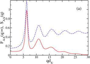
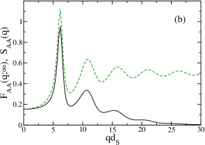
Figure 1: Non-decaying part of the large particles collective density correlation function, $F_{AA}(q;\infty)$ (solid line) compared to the large particles partial structure factor, $S_{AA}(q)$ (dashed line). Left panel (a): with particle size swaps; right panel (b): without swaps.

In the next set of figures we compare the non-decaying parts of the reduced, diagonal collective density correlations $F_{\alpha\alpha}(q;\infty)/S_{\alpha\alpha}(q)$, $\alpha=A,B$ and tagged particle density fluctuations, $F_{\alpha\alpha}^{s}(q;\infty)$, obtained from the present theory, Figs. 2a-b, and from the standard mode-coupling theory, Figs. 3a-b. Now we clearly see the difference of the small wavevector behavior of the frozen-in collective density correlations discussed above. In addition, we see the qualitative difference between the non-decaying parts of the diagonal tagged particle density correlations $F_{\alpha\alpha}^{s}(q;\infty)$. The present theory predicts $\lim_{q\to 0}F_{\alpha\alpha}^{s}(q;\infty)/x_{\alpha}<1$ whereas within the standard mode-coupling approach the conservation of the number of the particles of each type leads to $\lim_{q\to 0}F_{\alpha}^{s}(q;\infty)/x_{\alpha}=1$.

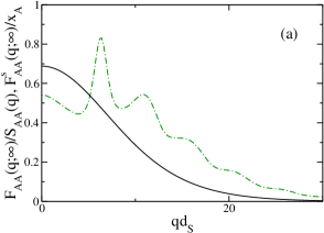
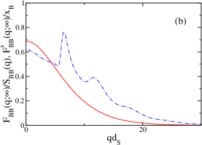
Figure 2: Particle size swap dynamics. Non-decaying part of the tagged particle density correlation function, $F_{\alpha\alpha}^{s}(q;\infty)/x_{\alpha}$ (solid line), compared to the corresponding normalized collective density correlation function, $F_{\alpha\alpha}^{s}(q;\infty)/S_{\alpha\alpha}(q)$ (dashed line). Left panel (a): $\alpha=A$; right panel (b): $\alpha=B$.

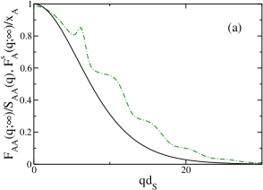
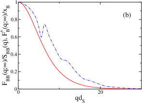
Figure 3: Dynamics without particle size swaps. Non-decaying part of the tagged particle density correlation function, $F_{\alpha}^{s}(q;\infty)/x_{\alpha}$ (solid line), compared to the corresponding normalized collective density correlation function, $F_{\alpha\alpha}(q;\infty)/S_{\alpha\alpha}(q)$ (dashed line). Left panel (a): $\alpha=A$; right panel (b): $\alpha=B$.

Following the spirit of Ikeda et al. [12, 13] we can use the small wavevector limits of the frozen-in tagged particle density correlations $F_{\alpha\alpha}^{s}(q;\infty)$ to define an order parameter for particle size swaps in the glass,

$$q=\lim_{q\to 0}\left[F_{AA}^{s}(q;\infty)-F_{AB}^{s}(q;\infty)-F_{BA}^{s}(q;\infty)+F_{BB}^{s}(q;\infty)\right],$$ (37)

where use the same symbol $q$ as in Refs. [12, 13] but caution the reader no to confuse this quantity with the wavevector $q$. The zero value of the order parameter, $q=0$ indicates the complete lack of particle type correlations in the glass whereas the maximum value, $q=1$, indicates the absence of the particle size swaps in the glass.

In Fig. 4a we show the volume fraction dependence of the particle size swaps order parameter for the diameter ratio at which the difference between these transitions is approximately the largest, $d_{L}/d_{S}=1.2$. On physical grounds one would expect the particle size swaps to become less probable with increasing volume fraction. The present theory confirms this expectation: we observe $q$ increasing monotonically starting from a nonzero value $q\approx 0.376$ at the dynamic glass transition. Qualitatively, the volume fraction dependence of the particle size swaps order parameter predicted by the present theory agrees with the prediction of the replica approach of Ikeda and Zamponi [13].

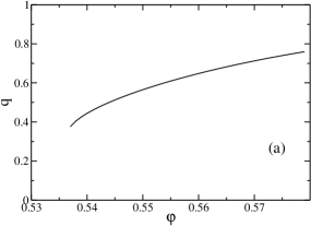
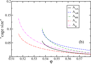
Figure 4: Left panel (a): order parameter for particle size swaps, $q$, as a function of the volume fraction, $\varphi$. Right panel (b): long-time limit of the mean square displacement (“cage size”) for the system with swap dynamics ($A_{\alpha\beta},\alpha,\beta=A,B$) and for the system without swaps ($A_{\alpha},\alpha=A,B$).

Within the standard mode-coupling theory, the small wavevector behavior of the frozen-in tagged particle density correlations $F_{\alpha}^{s}(q;\infty)$ allows one to define the long-time limit of the mean square displacement in the glass, which can be interpreted as a quantification of the “cage size”,

$$F_{\alpha}^{s}(q;\infty)=x_{\alpha}\left(1-\frac{1}{2}A_{\alpha}q^{2}/2+...\right)\;\text{ where }\;A_{\alpha}=\lim_{t\to\infty}\left<|\mathbf{r}_{1}^{\alpha}(t)-\mathbf{r}_{1}^{\alpha}(0)|^{2}\right>.$$

In the present case of a system with particle size swaps we generalize this definition as

$$F_{\alpha\beta}^{s}(q;\infty)=\sqrt{x_{\alpha}x_{\beta}}\left(1-\frac{1}{2}A_{\alpha\beta}q^{2}/2+...\right)$$

$$\;\;\;\;\;\;\;\;\;\;\text{ where }\;\;\;A_{\alpha\beta}=\lim_{t\to\infty}\left<|\mathbf{r}_{1}^{\alpha}(t)-\mathbf{r}_{1}^{\beta}(0)|^{2}\right>.$$ (39)

In Fig. 4b we show the volume fraction dependence of the $A_{\alpha\beta}$ and $A_{\alpha}$ for the diameter ratio at which the difference between these transitions is approximately the largest, $d_{L}/d_{S}=1.2$. As expected on physical grounds, all the quantities characterizing “cage size” decrease with increasing volume fraction. For a given volume fraction, the “cage size” for the system with particle size swaps is larger than that for the system without swaps. This is consistent with simulational results of Ninarello et al [6]. Furthermore, as expected on physical grounds, the cage size depends on the particle type and is smaller for the larger particles. Again, qualitatively, the volume fraction dependence of the “cage size” predicted by the present theory agrees with the prediction of the replica approach of Ikeda and Zamponi [13]. However, the important difference is that the latter theory uses only a single cage size parameter for both types of the particles, both in the system with particle size swaps and in the system without swaps.

6 Discussion

We presented here a theory for the single-particle motion in binary mixtures with particle size swaps. The present theory is an extension of the previously developed theory for the collective dynamics and the dynamic glass transition in binary mixtures with particle size swaps. Like the latter approach, the present theory is based on combination of a formally exact memory function representation of the tagged particle density correlation function and a factorization approximation for a four-point correlation function evolving with the irreducible dynamics. Thus, it belongs to the class of mode-coupling-like theories.

The present theory predicts that the single-particle motion becomes localized at the dynamic glass transition, like in the standard mode-coupling theory for systems with local dynamics only. The properties of the localized state are qualitatively similar to those of the localized state of a system with local dynamics only. The main difference is that at the same volume fraction the “cage size” is predicted to be larger in a system with particle size swaps than in the corresponding system without swaps.

The properties of the localized state predicted by the present theory are qualitatively similar to those predicted by the replica approach [13]. The main difference is that in our approach different “cage sizes” are obtained from the (approximate) calculation whereas the replica ansatz assumes that there is a single “cage size” parameter.

While solving numerically the time-dependent equations of motion for either collective or tagged particle density correlations seems difficult, it might be possible to re-do the standard mode-coupling asymptotic analysis and to check whether the power law approach to and departure from intermediate time plateaus are still present, and to check whether there is an analogue of the separation parameter determining the corresponding power laws exponents. This interesting problem is left for a future study.

References

- [1] L. Berthier and G. Biroli, Rev. Mod. Phys. 83, 587 (2011).
- [2] L. Berthier, P. Charbonneau, D. Coslovich, A. Ninarello, M. Ozawa, and S. Yaida, Proc. Natl. Acad. Sci. USA 114, 11356 (2017).
- [3] T. Grigera and G. Parisi, Phys. Rev. E 63, 045102(R) (2001).
- [4] See, e.g., E. Flenner and G. Szamel, Phys. Rev. E 73, 061505 (2006).
- [5] L. Berthier, D. Coslovich, A. Ninarello, and M. Ozawa, Phys. Rev. Lett. 116, 238002 (2016).
- [6] A. Ninarello, L. Berthier, and D. Coslovich, Phys. Rev. X 7, 021039 (2017).
- [7] M. Ozawa, L. Berthier, G. Biroli, A. Rosso and G. Tarjus, PNAS 115, 6656 (2018).
- [8] L. Wang, A. Ninarello, P. Guan, L. Berthier, G. Szamel and E. Flenner, Nature Communications 10, 26 (2019).
- [9] L. Berthier, P. Charbonneau, A. Ninarello, M. Ozawa and S. Yaida, arXiv:1805.09035.
- [10] M. Wyart and M.E. Cates, Phys. Rev. Lett. 119, 195501 (2017).
- [11] L. Berthier, G. Biroli, J.-P. Bouchaud, and G. Tarjus, arXiv:1805.12378.
- [12] H. Ikeda, F. Zamponi, and A. Ikeda, J. Chem. Phys. 147, 234506 (2017).
- [13] H. Ikeda and F. Zamponi, arXiv:1812.08780.
- [14] C. Brito, E. Lerner, and M. Wyart, Phys. Rev. X 8, 031050 (2018).
- [15] G. Kapteijns, W. Ji, C. Brito, M. Wyart, and E. Lerner, Phys. Rev. E 99 012106 (2019).
- [16] L. Berthier, E. Flenner, C.J. Fullerton, C. Scalliet, and M. Singh, arXiv:1811.12837.
- [17] G. Szamel, Phys. Rev. E 98, 050601(R) (2018).
- [18] W. Götze, Complex dynamics of glass-forming liquids: A mode-coupling theory (Oxford University Press, Oxford, 2008).
- [19] J.P. Hansen and I.R. McDonald, Theory of Simple Liquids (Elsevier, Amsterdam, 2006).
- [20] B. Cichocki and W. Hess, Physica A 141, 475 (1987).
- [21] K. Kawasaki, Physica A 215, 61 (1995).
- [22] G. Szamel and H. Löwen, Phys. Rev. A 44, 8215 (1991).
- [23] J.L. Lebowitz and J. S. Rowlinson, J. Chem. Phys. 41, 133 (1964).
- [24] R. J. Baxter, J. Chem. Phys. 52, 4559 (1970).
- [25] We used explicit formulas from Th. Voigtmann, Ph.D. thesis, TU München, 2002.
- [26] W. Götze and Th. Voigtmann, Phys. Rev. E 67, 021502 (2003).
- [27] We discretized the self-consistent equations (36) using a grid of 401 equally spaced wavevectors, with and , where is the diameter of the smaller sphere. The resulting equations were then solved by iteration, with integrations performed using a gaussian quadrature.