Improving Missing Data Imputation with Deep Generative Models

Abstract

Datasets with missing values are very common on industry applications, and they can have a negative impact on machine learning models. Recent studies introduced solutions to the problem of imputing missing values based on deep generative models. Previous experiments with Generative Adversarial Networks and Variational Autoencoders showed interesting results in this domain, but it is not clear which method is preferable for different use cases. The goal of this work is twofold: we present a comparison between missing data imputation solutions based on deep generative models, and we propose improvements over those methodologies. We run our experiments using known real life datasets with different characteristics, removing values at random and reconstructing them with several imputation techniques. Our results show that the presence or absence of categorical variables can alter the selection of the best model, and that some models are more stable than others after similar runs with different random number generator seeds.

1 Introduction

Analyzing data is a core component of scientific research across many domains. Over the recent years, awareness for the need of transparent and reproducible work increased. This includes all steps that involve preparing and pre-processing the data. An increasingly common pre-processing step is the imputation of missing values (Hayati Rezvan et al., 2015). Data with missing values can decrease model quality and even lead to wrong insights (Lall, 2016) by introducing biases. Likewise, dropping samples with missing values can cause larger errors because of the scarce amount of remaining data. One solution is performing data imputation, which consists in replacing missing values with substitutes. However, the reason behind the missingness needs to be clarified before imputing (Rubin, 1976). For example, (Lall, 2016) show that in political sciences, results often do not hold up if missing data is imputed improperly. Values are considered to be missing completely at random (MCAR) when the probability that they are missing is independent both on the value and on other observable values of the data. The case when data is missing at random (MAR) happens when the missing probability can be estimated from variables where the value is present. Finally, the case when missing data is neither MCAR nor MAR, is defined as missing not at random (MNAR). This means that the reason for a value to be missing, can depend on other variables, but also on the value that is missing. In order to be able to compare the desired models in the same framework, we assume for the this study that missing values are MCAR.

In this paper, we survey the quickly evolving state-of-the-art of deep generative models for tabular data and missing value imputation. We propose using a backpropagation technique to correct the imputed values iteratively. We also adapt the analyzed models by changing the inputs and outputs of the architectures, taking into account the size and the type of each sample variable. Furthermore, we compare the imputation power of every technique using real life datasets.

2 Related Work

Work related to our approach falls into three groups. The first one consists of state-of-the-art imputation algorithms. The second group is composed by generative models based in neural networks, and in particular, networks focusing on generating tabular data and handling issues related to categorical variables, rather than generating one high-dimensional image or text variable. Lastly, the third group is constituted by methodologies using deep generative models for imputation in the domain of tabular data.

Within the field of missing value imputation, traditional methods can be classified into discriminative and generative imputation models. Examples of discriminative models with state-of-the-art performance are MICE (Buuren & Groothuis-Oudshoorn, 2010), MissForest (Stekhoven & Bühlmann, 2011), and Matrix Completion (Mazumder et al., 2010). Autoencoders (Gondara & Wang, 2017) and Expectation Maximization (García-Laencina et al., 2010) are instances of generative models. Key distinguishing factors of these methods are limitations coming from necessary assumptions about the nature and distribution of the data and the ability to learn from samples with missing data (rather than only learning from complete data samples).

Deep generative models like Variational Autoencoders (VAE) (Kingma & Welling, 2013a) and Generative Adversarial Networks (GAN) (Goodfellow et al., 2014) proved to be very powerful in the domain of computer vision (Brock et al., 2018), speech recognition and natural language processing (Jain et al., 2017; Lin et al., 2017). It is expected for the scientific community to extend the application of these models to other areas. The authors of medGAN (Choi et al., 2017) applied GANs to generate synthetic health care patient records represented by numerical and binary features. The multi-categorical GANs (Camino et al., 2018) extended medGAN and other architectures by splitting the outputs of the networks into parallel layers depending on the size of categorical variables, and used gumbel-softmax activations (Jang et al., 2016; Maddison et al., 2016) to handle discrete distributions. (Mottini et al., 2018) proposed a GAN based architecture to generate synthetic passenger name records, dealing with missing values and a mix of categorical and numerical variables. Tabular GAN (TGAN) (Xu & Veeramachaneni, 2018) presented a method to generate data composed by numerical and categorical variables, where the generator outputs variable values in an ordered sequence using a recurrent neural network architecture.

There are numerous studies related to image completion with deep generative models like (Vincent et al., 2008), that uses denoising autoencoders for image imputing. In the domain of natural language processing, (Bowman et al., 2015) presented a VAE model with a recurrent architecture for sentence generation and imputation. This use case was also translated to the topic of missing value imputation on tabular data. Generative Adversarial Imputation Nets (GAIN) (Yoon et al., 2018) adapted the GAN architecture to this problem and proved to be more efficient than state-of-the-art imputation methods. The Heterogeneous-Incomplete VAE (HI-VAE) (Nazabal et al., 2018) proposed an imputation technique for tabular data based on VAE, and also compared their results to state-of-the-art imputation methodologies.

3 Approach

3.1 Problem Definition

We define a tabular dataset $X$ as a collection of samples $\{x_{1},\ldots,x_{n}\}$. Each sample $x_{i}$ is a collection of values $\{v_{i1},\ldots,v_{im}\}$ for the variables $\{V_{1},\ldots,V_{m}\}$, where each variable $V_{j}$ has a type $t_{j}\in\{$numerical, categorical$\}$. The value of a numerical variable $V_{j}$ is represented only by one real valued feature, hence we define the size of a numerical variable as $s_{j}=1$. A categorical variable $V_{j}$ can take one of $s_{j}>1$ possible categories. We one-hot encode each value $v_{ij}$ into $s_{j}$ binary features, by turning on the feature corresponding to the selected category and turning off the remaining $s_{j}-1$ features. Combining the amount of features of each variable, we define the amount of features (or size) of every sample as $s=\sum_{j=1}^{m}s_{j}$.

We can now define a dataset with missing values $\bar{X}$ as a copy of a dataset $X$ where one or more variable values from one or more samples were dropped. An imputation algorithm or model $\mathcal{M}$ takes a dataset with missing values $\bar{X}$ and outputs a dataset $\hat{X}$ by filling the missing values of $\bar{X}$. The goal of these algorithms is to minimize the difference between the original dataset $X$ and its reconstructed version $\hat{X}$.

In addition, we define a the mask $M$ of $\bar{X}$ that will be used in the following method definitions. We represent $M$ as a matrix $\in\{0,1\}^{n\times s}$, where each position $m_{ik}$ contains a 1 if the feature on $\bar{x}_{ik}$ is present or a 0 if it is missing. Also for the training of deep learning models, we note subset of sample indices $B\subset\{1,\ldots,n\}$ as a mini-batch.

3.2 Gumbel-Softmax

The output of a neural network can be transformed into a multinominal distribution by passing it through a softmax layer. However, sampling from this distribution is not a differentiable operation, which blocks the backpropagation during the training of generative models for discrete samples. The Gumbel-Softmax (Jang et al., 2016) and the Concrete-Distribution (Maddison et al., 2016) were simultaneously proposed to tackle this problem in the domain of variational autoencoders (VAE) (Kingma & Welling, 2013b). Later (Kusner & Hernández-Lobato, 2016) adapted the technique to GANs for sequences of discrete elements.

For i.i.d samples $g_{1},\ldots,g_{d}$ drawn from $Gumbel(0,1)=-\log(-\log(u_{i}))$ with $u_{i}\sim U(0,1)$, the gumbel-softmax generates sample vectors $b\in\left[0,1\right]^{d}$ based on inputs $a\in R^{d}$ (that can be the output of previous layers) and a temperature hyperparameter $\tau\in(0,\infty)$ by the formula:

$$\begin{array}[]{rl}b_{i}=\dfrac{exp((\log(a_{i})+g_{i})/\tau)}{\sum_{j=1}^{d}exp((\log(a_{j})+g_{j})/\tau)}&i=1,\ldots,d\end{array}$$

3.3 GAIN

GAIN (Yoon et al., 2018) is composed of a modified generator and discriminator network. Compared to the original GAN architecture (Goodfellow et al., 2014), the differences are as follows: The generator $G$ takes as input some data $\bar{X}$, a suitable mask $M$, and a source of noise. In practice, the noise is inserted inside $\bar{X}$ in the positions of the missing values. The model then returns an imputation $\hat{X}$.
The discriminator $D$ of the GAN architecture receives $\hat{X}$, and instead of trying to determine if each sample from the input is either real or fake, the model tries guess for every sample if each variable value is either original or imputed. In other words, the discriminator needs to be trained to maximize the probability of predicting the mask $M$. Hence, we note the output of network $D$ as $\hat{M}$. The discriminator loss only takes into account the binary cross entropy of the positions corresponding to missing values:

$$\mathcal{L}_{D}(M_{i},\hat{M}_{i})=-\sum_{k=1}^{s}m_{ik}\log\hat{m}_{ik}+(1-m_{ik})\log(1-\hat{m}_{ik})$$

for every sample $i$. Then, for a mini-batch $B$, the discriminator $D$ with parameters $\theta_{D}$ is trained to optimize:

$$\min_{\theta_{D}}\sum_{i\in B}\mathcal{L}_{D}(M_{i},\hat{M}_{i})$$

Given that $\hat{M}=D(\hat{X})$ and $\hat{X}=G(\bar{X},M)$, the generator $G$ with parameters $\theta_{G}$ is trained to maximize the probability of fooling the discriminator predictions of $M$:

$$\mathcal{L}_{G}(M_{i},\hat{M}_{i})=-\sum_{k=1}^{s}(1-m_{ik})\log\hat{m}_{ik}$$

$$\min_{\theta_{G}}\sum_{i\in B}\mathcal{L}_{G}(M_{i},\hat{M}_{i})+\alpha\mathcal{L}_{rec}(\bar{X}_{i},\hat{X}_{i},M_{i})$$

where $\mathcal{L}_{rec}(\bar{X}_{i},\hat{X}_{i},M_{i})$ is a special reconstruction loss term weighted by the hyperparameter $\alpha$. This loss function is separated by variable and masked in order to calculate only the reconstruction error for the non-missing values:

$$\mathcal{L}_{rec}(\bar{X}_{i},\hat{X}_{i},M_{i})=\sum_{j=1}^{m}\sum_{q=1}^{s_{j}}m_{ik}rec_{j}(\bar{x}_{ik},\hat{x}_{ik})$$ (1)

where the feature index $k$ is calculated as:

$$k=\sum_{j^{\prime}=0}^{j-1}s_{j^{\prime}}+q-1$$

which is the index for the first feature of $v_{j}$ plus the offset for the categorical value $q$ (or no offset for numerical variables). The reconstruction error for each feature of a particular variable $v_{j}$ depends on the variable type $t_{j}$:

$$rec_{j}(\bar{x}_{ik},\hat{x}_{ik})=\left\{\begin{array}[]{ll}\left(\hat{x}_{ik}-\bar{x}_{ik}\right)^{2}&\text{if }t_{j}\text{ = numerical}\\ -\bar{x}_{ik}\log\hat{x}_{ik}&\text{if }t_{j}\text{ = categorical}\end{array}\right.$$

3.4 VAE Imputation

We train a traditional VAE (Kingma & Welling, 2013a) using $\bar{X}_{train}$ as input, but inserting random noise on the positions with missing values. We use the masked the reconstruction loss defined in Equation 1 to calculate the reconstruction error between $\hat{X}_{train}$ and $X_{train}$ only on the non-missing values. We use the trained model to obtain $\hat{X}_{test}$ from $\bar{X}_{test}$ and use the reconstructed missing values for imputation.

3.5 VAE Iterative Imputation

The method from (McCoy et al., 2018) is an extension of the VAE imputation, related to the iterative PCA imputation algorithm (Dray & Josse, 2015). The training stage remains the same, but the imputation procedure is corrected iteratively. The reconstruction error of the non-missing values is measured after each iteration, and if the error is small enough or too many iterations have been calculated, the algorithm stops. If the procedure must continue, $\bar{X}_{test}$ is run through the model again, but instead of inserting random noise on the positions with missing values, the reconstructed missing values from the previous iteration are used. Note that it makes no sense to use the reconstruction error of the missing values as a stopping criteria, because in a real case scenario, the missing values are supposed to be unknown. A pseudocode for this method is presented in Algorithm 1.

Algorithm 1 VAE Iterative Imputation

  Input: $\bar{X}_{train}$ data with missing values for training

  Input: $M_{train}$ mask for $\bar{X}_{train}$

  Input: $\bar{X}_{test}$ data with missing values to impute

  Input: $M_{test}$ mask for $\bar{X}_{test}$

  Input: $i_{max}$ maximum number of iterations

  Input: $e_{min}$ minimum error

  Output: $\hat{X}_{test}$ imputation of $\bar{X}_{test}$

  $VAE=train(\bar{X}_{train},M_{train})$

  $\epsilon\sim\mathcal{N}(0,1)^{sizeof(M_{test})}$

  $\hat{X}_{test}=\bar{X}_{test}*M_{test}+\epsilon*(1-M_{test})$

  $i=0$

  repeat

     $\hat{X}_{test}=VAE(\hat{X}_{test})$

     $e=\mathcal{L}_{rec}(\bar{X}_{test},\hat{X}_{test},M_{test})$

     $\hat{X}_{test}=\bar{X}_{test}*M_{test}+\hat{X}_{test}*(1-M_{test})$

     $i++$

  until $e\leq e_{min}$ or $i\geq i_{max}$

3.6 VAE Backpropagation Imputation

The thrid VAE technique is an altered form of the iterative imputation: on each iteration, the reconstruction error of the non-missing values is backpropagated to the input. Instead of updating the weights of the model like in a traditional training, the noise itself is updated, keeping the model and the non-missing values untouched. The stopping criteria remains the same: the algorithm iterates until the error is sufficiently small or the number of iterations is large enough. This technique is inspired by (Schlegl et al., 2017), where the authors detect anomalies on images by searching through the latent space used as input for the generator. A pseudocode for this method is presented in Algorithm 2, highlighting the differences with Algorithm 1.

Algorithm 2 VAE Iterative Backpropagation Imputation

  Input: $\bar{X}_{train}$ data with missing values for training

  Input: $M_{train}$ mask for $\bar{X}_{train}$

  Input: $\bar{X}_{test}$ data with missing values to impute

  Input: $M_{test}$ mask for $\bar{X}_{test}$

  Input: $i_{max}$ maximum number of iterations

  Input: $e_{min}$ minimum error

  Output: $\hat{X}_{test}$ imputation of $\bar{X}_{test}$

  $VAE=train(\bar{X}_{train},M_{train})$

  $\epsilon\sim\mathcal{N}(0,1)^{sizeof(M_{test})}$

  $\hat{X}_{test}=\bar{X}_{test}*M_{test}+\epsilon*(1-M_{test})$

  $i=0$

  repeat

     $\hat{X}_{test}=VAE(\hat{X}_{test})$

     $e=\mathcal{L}_{rec}(\bar{X}_{test},\hat{X}_{test},M_{test})$

      $grads=backprop(e)$

      $\hat{X}_{test}=optim(\hat{X}_{test},grads)$

     $\hat{X}_{test}=\bar{X}_{test}*M_{test}+\hat{X}_{test}*(1-M_{test})$

     $i++$

  until $e\leq e_{min}$ or $i\geq i_{max}$

3.7 Variable Splitting

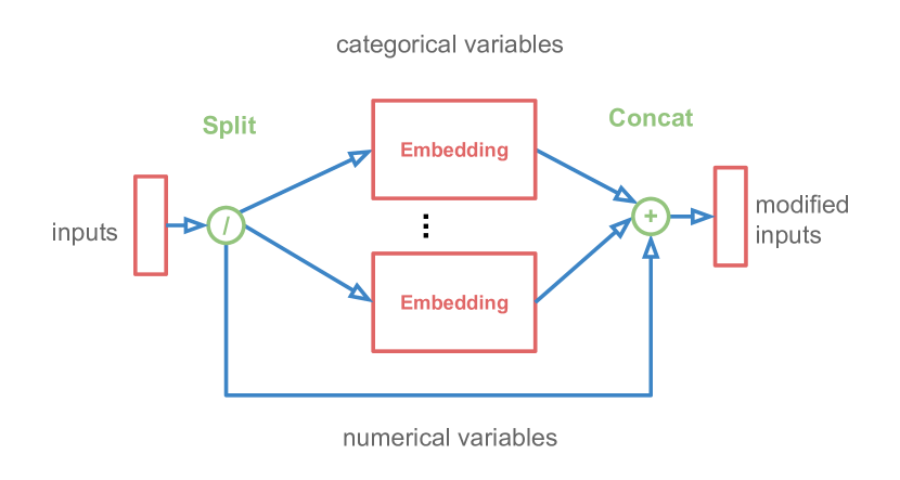
Figure 1: Architecture for splitting input variables.

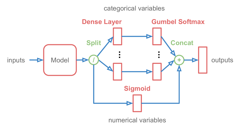
Figure 2: Architecture for splitting output variables.

The authors of multi-output GANs (Camino et al., 2018) introduced the notion of taking into account the structure of categorical variables from tabular data to modify the network architecture. A multi-output GAN contains one dense layer per variable connected in parallel to the output of the generator. Each dense layer transforms the output to the size of the corresponding variable. A gumbel-softmax activation (Jang et al., 2016) (or concrete distribution (Maddison et al., 2016)) is used after each parallel dense layer. All the outputs are concatenated back into a complete synthetic sample. The work on (Camino et al., 2018) also extended other GAN architectures involving autoencoders (Junbo et al., 2017; Choi et al., 2017), where the decoder is the altered model with multiple outputs, and the generator returns continuous latent codes for the autoencoders. In this study we extend multi-output architecture in two ways:

• We work with tabular data of mixed numerical and categorical variables. In order to do so, during the splitting of numerical variables, we do not apply size transformations with dense layers, but we apply sigmoid activations before concatenating the output. The changes can be observed on Figure 2. This extends (Camino et al., 2018) to settings with mixed numerical and categorical data.

• We transfer the idea to the inputs too, by using one embedding layer per categorical variable with the corresponding size of each variable.The outputs of each parallel embedding layer are concatenated back to build the altered inputs. Numerical variables are concatenated directly with the outputs of the embeddings. Related architectures and applications can be found in (Weston et al., 2011; De Brébisson et al., 2015). A representation can be seen on Figure 1.

We propose to modify the GAIN architecture by adding the multiple-inputs and multiple-outputs both to the generator and the discriminator. For the VAE, we propose to use multi-input on the encoder and multi-output on the decoder.

4 Experiments

Table 1: Dataset properties.

Name	Samples	Features	Variables	Numerical	Categorical
breast cancer	569	30	30	30	0
default credit card	30000	93	23	14	9
letter recognition	20000	16	16	16	0
online news popularity	39644	60	47	44	3
spambase	4601	57	57	57	0

4.1 Data and Pre-Processing

We evaluate the presented imputation methods using five real life datasets from the UCI repository (Dheeru & Karra Taniskidou, 2017). They are composed of different number of samples and variables, both categorical and numerical. Originally, no dataset contains missing values. A summary of their properties is defined in Table 1.

For all datasets, categorical variables are one-hot encoded, and each numerical variable $V_{j}$ is scaled to fit inside the interval $[0,1]$ according to the equation:

$$scaled(V_{j})=\frac{V_{j}-\min(V_{j})}{\max(V_{j})-\min(V_{j})}$$

where $\max(V_{j})$ and $\min(V_{j})$ are the maximum and minimum values for the variable $V_{j}$ from all samples that can be measured across the entire dataset.

4.2 Running the Experiments

All the experiments are implemented using Python 2.7.15, PyTorch 0.4.0 (Paszke et al., 2017) and scikit-learn 0.19.1 (Pedregosa et al., 2011). The code is available in the supplementary material. After the review process, we plan to port the implementation to Python 3 and release it to the public.

All models are trained with 90% of the original data and the other 10% is used to evaluate the performance of the imputation methods. We generate different settings of missing value probabilities $p\in\{0.2,0.5,0.8\}$. Given a missing probability $p$, each variable of each sample is dropped if $r<p$, for a random number $r\sim\mathcal{U}[0,1]$. The value of a dropped variable is replaced by random noise $\mathcal{N}(0,1)$.

Each method has different amount of hyperparameters that need to be defined. For GAIN, we use the same configuration defined in (Yoon et al., 2018), and we only experiment with different values for the weight of the reconstruction loss as the authors did originally. Across all our experiments we get the best results with a value of 10. We perform a random search for the hyperparameters needed by the VAE based methods. Both the encoder’s and the decoder’s hidden layers (beside the special input and output layers) are implemented as a collection of fully connected layers with ReLU activations. We experiment with one hidden layer with 50% of the input size, two layers with 100% and 50% of the input size respectively, and no hidden layers at all. For the size of the latent space, we tried with 10%, 50% and 100% of the input size. Other learning hyperparameters include the batch size, for which we explored the values $\{2^{6},2^{7},2^{8},2^{9},2^{10}\}$, and two different learning rates of $1e^{-3}$ and $1e^{-5}$. Both of the iterative imputation also need to define the maximum number of iterations and the minimum acceptable error to stop, for which we fix 10000 iterations and $1e^{-4}$. Finally, the variable split adapted architectures use gumbel-softmax activations, and we experiment with the temperature or $\tau$ hyperparameter using the values $\{0.1,0.5,1,2,10\}$.

Furthermore, every experiment is repeated at least three times using different seeds on the random number generator. For each collection of experiments that differ only on the seed, we calculate the mean and the standard deviation of the Root Mean Squared Error (RMSE) between the (normalized) imputed and the original test data values.

4.3 Results

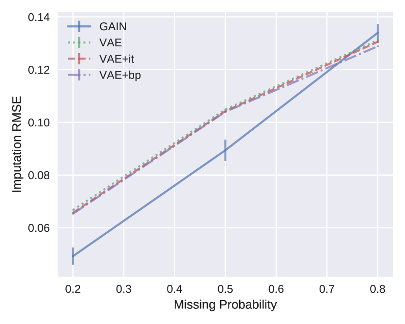
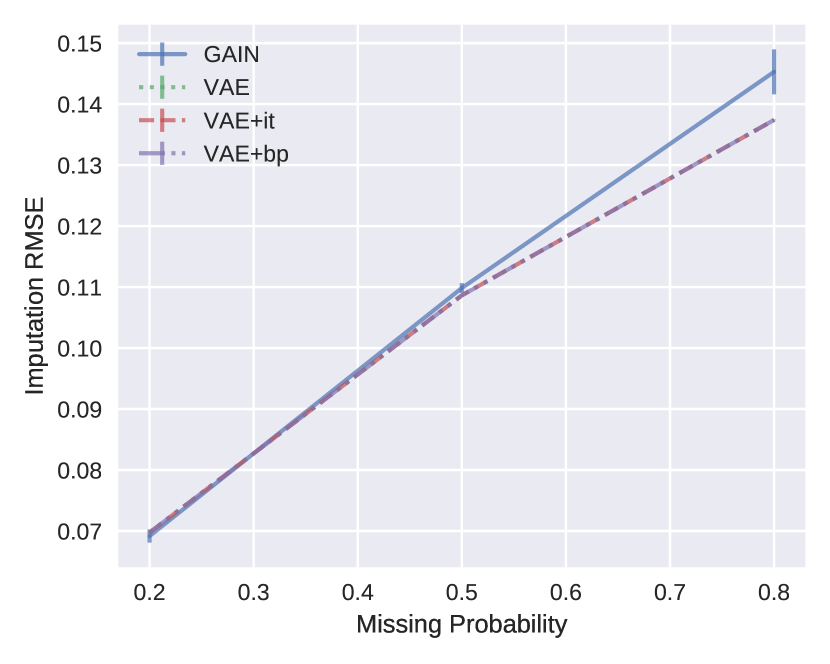
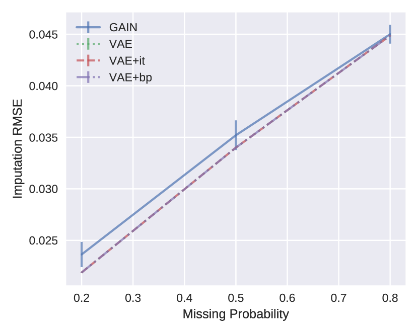
Figure 3: Imputation RMSE by increasing proportion of missing values for the Breast Cancer, Letter Recognition and Spambase datasets.

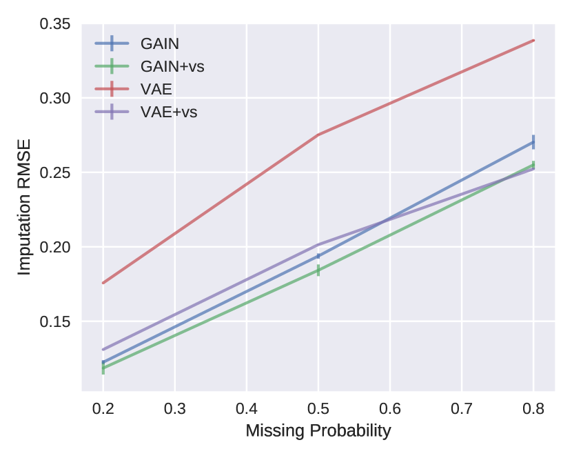
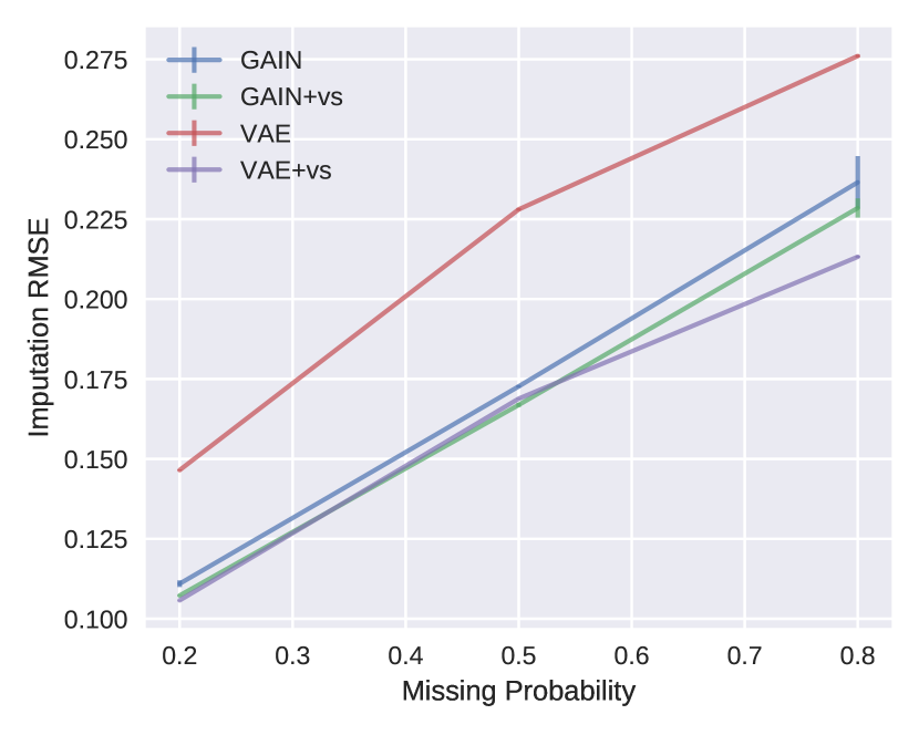
Figure 4: Imputation RMSE by increasing proportion of missing values for the Default Credit Card and Online News Popularity datasets.

Table 2: Imputation for datasets with numerical variables only.

Breast Cancer
Missing	20%	50%	80%
GAIN	$0.049\pm 0.003$	$0.089\pm 0.004$	$0.134\pm 0.003$
VAE	$0.067\pm 0.000$	$0.105\pm 0.000$	$0.131\pm 0.000$
VAE+it	$0.066\pm 0.000$	$0.104\pm 0.000$	$0.131\pm 0.000$
VAE+bp	$0.065\pm 0.000$	$0.104\pm 0.000$	$0.129\pm 0.000$
Letter Recognition
Missing	20%	50%	80%
GAIN	$0.069\pm 0.001$	$0.110\pm 0.001$	$0.145\pm 0.004$
VAE	$0.070\pm 0.000$	$0.109\pm 0.000$	$0.137\pm 0.000$
VAE+it	$0.070\pm 0.000$	$0.109\pm 0.000$	$0.137\pm 0.000$
VAE+bp	$0.070\pm 0.000$	$0.109\pm 0.000$	$0.137\pm 0.000$
Spambase
Missing	20%	50%	80%
GAIN	$0.024\pm 0.001$	$0.035\pm 0.001$	$0.045\pm 0.001$
VAE	$0.022\pm 0.000$	$0.034\pm 0.000$	$0.045\pm 0.000$
VAE+it	$0.022\pm 0.000$	$0.034\pm 0.000$	$0.045\pm 0.000$
VAE+bp	$0.022\pm 0.000$	$0.034\pm 0.000$	$0.045\pm 0.000$

Table 3: Imputation for datasets with mixed variable types.

Default Credit Card
Missing	20%	50%	80%
GAIN	$0.123\pm 0.001$	$0.194\pm 0.002$	$0.270\pm 0.005$
GAIN+vs	$0.119\pm 0.004$	$0.184\pm 0.004$	$0.255\pm 0.003$
VAE	$0.176\pm 0.000$	$0.275\pm 0.000$	$0.339\pm 0.000$
VAE+it	$0.176\pm 0.000$	$0.275\pm 0.000$	$0.339\pm 0.000$
VAE+bp	$0.176\pm 0.000$	$0.275\pm 0.000$	$0.339\pm 0.000$
VAE+vs	$0.131\pm 0.000$	$0.201\pm 0.000$	$0.252\pm 0.000$
VAE+vs+it	$0.131\pm 0.000$	$0.201\pm 0.000$	$0.252\pm 0.000$
VAE+vs+bp	$0.131\pm 0.000$	$0.201\pm 0.000$	$0.252\pm 0.000$
Online News Popularity
Missing	20%	50%	80%
GAIN	$0.111\pm 0.001$	$0.173\pm 0.000$	$0.237\pm 0.008$
GAIN+vs	$0.107\pm 0.000$	$0.167\pm 0.001$	$0.228\pm 0.003$
VAE	$0.146\pm 0.000$	$0.228\pm 0.000$	$0.276\pm 0.000$
VAE+it	$0.146\pm 0.000$	$0.228\pm 0.000$	$0.276\pm 0.000$
VAE+bp	$0.146\pm 0.000$	$0.228\pm 0.000$	$0.276\pm 0.000$
VAE+vs	$0.106\pm 0.000$	$0.169\pm 0.000$	$0.213\pm 0.000$
VAE+vs+it	$0.106\pm 0.000$	$0.169\pm 0.000$	$0.213\pm 0.000$
VAE+vs+bp	$0.106\pm 0.000$	$0.169\pm 0.000$	$0.213\pm 0.000$

For the following experiments, we use the notation “+vs” for variable split, “+it” for iterative imputation and “+bp” for backpropagation iterative imputation. In Figure 3 we present the imputation RMSE by increasing proportion of missing values for datasets with only numerical variables, and in Figure 4 the rest of the datasets that contain both numerical and categorical variables. For the sake of clarity, we removed the iterative imputation methods from Figure 4. Nevertheless, a full description of the imputation results can be seen on Tables 2 and 3. From the plots and the tables we can extract the following observations:

• As expected, the performance of every model decreases when the proportion of missing values increases.

• The iterative and backpropagation alternatives for the VAE imputation do not seem to add improvements over the plain VAE imputation.

• For the datasets with only numerical variables, GAIN seems to be better for the smaller dataset, but it is slightly worse than VAE for the other bigger datasets.

• The variable splitting appears improve both models, but the improvement is more drastic in the case of VAE.

• GAIN has some perceptible variance when trained with different seeds, but all VAE methods seems to be more stable, even when they have worse performance.

4.4 Discussion

Deep generative models for missing data imputation proved to surpass state-of-the-art methods in previous studies (Yoon et al., 2018; Nazabal et al., 2018). However, the power these models offer come at some cost. The number of hyperparameters to tune is usually larger than traditional non deep learning solutions. The training time or memory size required for the hyperparameter search using large datasets can be prohibitive in some cases. Furthermore, the amount of research papers on this domain is growing rapidly, but in many cases, the matching code is either not available or incomplete. In comparison, traditional methods are well established in the scientific community. This can lead practitioners to rely on known and robust libraries instead of implementing deep learning alternatives themselves.

5 Conclusion

In this paper, we compare several deep generative models for missing data imputation on tabular data, and we propose improvements on top of each model to further improve their imputation quality: first, using variable splitting to account for categorical variables, and second, an iterative backpropagation-based method for VAEs.

Our experiments with public datasets show that our proposals match and improve the performance of deep generative models, which already were shown to outperform state-of-the-art imputation methods in the literature.

Adding variable splitting techniques to separate variables, applied both on the inputs and the outputs, enhances the imputation power of GAIN and all the presented variants of VAE. In contrast, both of the VAE iterative imputation procedures did not significantly increase the quality of imputations compared with the basic VAE model.

To support reproducible research, we provide open implementations for our research by making our code public . We are looking forward to collaborate both with developers and the scientific community.

Acknowledgments

The experiments presented in this paper were carried out using the HPC facilities of the University of Luxembourg (Varrette et al., 2014) – see https://hpc.uni.lu.

References

- Bowman et al. (2015) Bowman, S. R., Vilnis, L., Vinyals, O., Dai, A. M., Jozefowicz, R., and Bengio, S. Generating sentences from a continuous space. arXiv preprint arXiv:1511.06349, 2015.
- Brock et al. (2018) Brock, A., Donahue, J., and Simonyan, K. Large scale GAN training for high fidelity natural image synthesis. arXiv:1809.11096 [cs, stat], 2018. URL http://arxiv.org/abs/1809.11096.
- Buuren & Groothuis-Oudshoorn (2010) Buuren, S. v. and Groothuis-Oudshoorn, K. mice: Multivariate imputation by chained equations in r. Journal of statistical software, pp. 1–68, 2010.
- Camino et al. (2018) Camino, R., Hammerschmidt, C., and State, R. Generating multi-categorical samples with generative adversarial networks. arXiv preprint arXiv:1807.01202, 2018.
- Choi et al. (2017) Choi, E., Biswal, S., Malin, B., Duke, J., Stewart, W. F., and Sun, J. Generating Multi-label Discrete Patient Records using Generative Adversarial Networks. arXiv:1703.06490 [cs], March 2017. URL http://arxiv.org/abs/1703.06490. arXiv: 1703.06490.
- De Brébisson et al. (2015) De Brébisson, A., Simon, É., Auvolat, A., Vincent, P., and Bengio, Y. Artificial neural networks applied to taxi destination prediction. arXiv preprint arXiv:1508.00021, 2015.
- Dheeru & Karra Taniskidou (2017) Dheeru, D. and Karra Taniskidou, E. UCI machine learning repository, 2017. URL http://archive.ics.uci.edu/ml.
- Dray & Josse (2015) Dray, S. and Josse, J. Principal component analysis with missing values: a comparative survey of methods. Plant Ecology, 216(5):657–667, 2015.
- García-Laencina et al. (2010) García-Laencina, P. J., Sancho-Gómez, J.-L., and Figueiras-Vidal, A. R. Pattern classification with missing data: a review. Neural Computing and Applications, 19(2):263–282, 2010.
- Gondara & Wang (2017) Gondara, L. and Wang, K. Multiple imputation using deep denoising autoencoders. arXiv preprint arXiv:1705.02737, 2017.
- Goodfellow et al. (2014) Goodfellow, I., Pouget-Abadie, J., Mirza, M., Xu, B., Warde-Farley, D., Ozair, S., Courville, A., and Bengio, Y. Generative adversarial nets. In Advances in neural information processing systems, pp. 2672–2680, 2014.
- Hayati Rezvan et al. (2015) Hayati Rezvan, P., Lee, K. J., and Simpson, J. A. The rise of multiple imputation: a review of the reporting and implementation of the method in medical research. BMC Medical Research Methodology, 15, 2015. ISSN 1471-2288. doi: 10.1186/s12874-015-0022-1. URL https://www.ncbi.nlm.nih.gov/pmc/articles/PMC4396150/.
- Jain et al. (2017) Jain, U., Zhang, Z., and Schwing, A. G. Creativity: Generating diverse questions using variational autoencoders. CoRR, abs/1704.03493, 2017. URL http://arxiv.org/abs/1704.03493.
- Jang et al. (2016) Jang, E., Gu, S., and Poole, B. Categorical Reparameterization with Gumbel-Softmax. arXiv:1611.01144 [cs, stat], November 2016. URL http://arxiv.org/abs/1611.01144. arXiv: 1611.01144.
- Junbo et al. (2017) Junbo, Zhao, Kim, Y., Zhang, K., Rush, A. M., and LeCun, Y. Adversarially Regularized Autoencoders. arXiv:1706.04223 [cs], June 2017. URL http://arxiv.org/abs/1706.04223. arXiv: 1706.04223.
- Kingma & Welling (2013a) Kingma, D. P. and Welling, M. Auto-encoding variational bayes. arXiv preprint arXiv:1312.6114, 2013a.
- Kingma & Welling (2013b) Kingma, D. P. and Welling, M. Auto-Encoding Variational Bayes. arXiv:1312.6114 [cs, stat], December 2013b. URL http://arxiv.org/abs/1312.6114. arXiv: 1312.6114.
- Kusner & Hernández-Lobato (2016) Kusner, M. J. and Hernández-Lobato, J. M. GANS for Sequences of Discrete Elements with the Gumbel-softmax Distribution. arXiv:1611.04051 [cs, stat], November 2016. URL http://arxiv.org/abs/1611.04051. arXiv: 1611.04051.
- Lall (2016) Lall, R. How multiple imputation makes a difference. Political Analysis, 24(4):414–433, 2016. ISSN 1047-1987, 1476-4989. doi: 10.1093/pan/mpw020. URL https://www.cambridge.org/core/product/identifier/S1047198700014145/type/journal_article.
- Lin et al. (2017) Lin, K., Li, D., He, X., Zhang, Z., and Sun, M. Adversarial ranking for language generation. CoRR, abs/1705.11001, 2017. URL http://arxiv.org/abs/1705.11001.
- Maddison et al. (2016) Maddison, C. J., Mnih, A., and Teh, Y. W. The Concrete Distribution: A Continuous Relaxation of Discrete Random Variables. arXiv:1611.00712 [cs, stat], November 2016. URL http://arxiv.org/abs/1611.00712. arXiv: 1611.00712.
- Mazumder et al. (2010) Mazumder, R., Hastie, T., and Tibshirani, R. Spectral regularization algorithms for learning large incomplete matrices. Journal of machine learning research, 11(Aug):2287–2322, 2010.
- McCoy et al. (2018) McCoy, J. T., Kroon, S., and Auret, L. Variational autoencoders for missing data imputation with application to a simulated milling circuit. IFAC-PapersOnLine, 51(21):141–146, 2018.
- Mottini et al. (2018) Mottini, A., Lheritier, A., and Acuna-Agost, R. Airline passenger name record generation using generative adversarial networks. arXiv preprint arXiv:1807.06657, 2018.
- Nazabal et al. (2018) Nazabal, A., Olmos, P. M., Ghahramani, Z., and Valera, I. Handling incomplete heterogeneous data using vaes. arXiv preprint arXiv:1807.03653, 2018.
- Paszke et al. (2017) Paszke, A., Gross, S., Chintala, S., Chanan, G., Yang, E., DeVito, Z., Lin, Z., Desmaison, A., Antiga, L., and Lerer, A. Automatic differentiation in pytorch. 2017.
- Pedregosa et al. (2011) Pedregosa, F., Varoquaux, G., Gramfort, A., Michel, V., Thirion, B., Grisel, O., Blondel, M., Prettenhofer, P., Weiss, R., Dubourg, V., Vanderplas, J., Passos, A., Cournapeau, D., Brucher, M., Perrot, M., and Duchesnay, E. Scikit-learn: Machine learning in Python. Journal of Machine Learning Research, 12:2825–2830, 2011.
- Rubin (1976) Rubin, D. B. Inference and missing data. Biometrika, 63(3):581–592, 1976.
- Schlegl et al. (2017) Schlegl, T., Seeböck, P., Waldstein, S. M., Schmidt-Erfurth, U., and Langs, G. Unsupervised anomaly detection with generative adversarial networks to guide marker discovery. In International Conference on Information Processing in Medical Imaging, pp. 146–157. Springer, 2017.
- Stekhoven & Bühlmann (2011) Stekhoven, D. J. and Bühlmann, P. Missforest—non-parametric missing value imputation for mixed-type data. Bioinformatics, 28(1):112–118, 2011.
- Varrette et al. (2014) Varrette, S., Bouvry, P., Cartiaux, H., and Georgatos, F. Management of an academic hpc cluster: The ul experience. In Proc. of the 2014 Intl. Conf. on High Performance Computing & Simulation (HPCS 2014), pp. 959–967, Bologna, Italy, July 2014. IEEE.
- Vincent et al. (2008) Vincent, P., Larochelle, H., Bengio, Y., and Manzagol, P.-A. Extracting and composing robust features with denoising autoencoders. In Proceedings of the 25th international conference on Machine learning, pp. 1096–1103. ACM, 2008.
- Weston et al. (2011) Weston, J., Bengio, S., and Usunier, N. Wsabie: Scaling up to large vocabulary image annotation. In IJCAI, volume 11, pp. 2764–2770, 2011.
- Xu & Veeramachaneni (2018) Xu, L. and Veeramachaneni, K. Synthesizing tabular data using generative adversarial networks. arXiv preprint arXiv:1811.11264, 2018.
- Yoon et al. (2018) Yoon, J., Jordon, J., and van der Schaar, M. Gain: Missing data imputation using generative adversarial nets. arXiv preprint arXiv:1806.02920, 2018.