Linear Time Visualization and Search in Big Data using Pixellated Factor Space Mapping

Abstract

It is demonstrated how linear computational time and storage efficient approaches can be adopted when analyzing very large data sets. More importantly, interpretation is aided and furthermore, basic processing is easily supported. Such basic processing can be the use of supplementary, i.e. contextual, elements, or particular associations. Furthermore pixellated grid cell contents can be utilized as a basic form of imposed clustering. For a given resolution level, here related to an associated m-adic ($m$ here is a non-prime integer) or p-adic ($p$ is prime) number system encoding, such pixellated mapping results in partitioning. The association of a range of m-adic and p-adic representations leads naturally to an imposed hierarchical clustering, with partition levels corresponding to the m-adic-based and p-adic-based representations and displays. In these clustering embedding and imposed cluster structures, some analytical visualization and search applications are described.

Fionn Murtagh, University of Huddersfield, fmurtagh@acm.org

1 Introduction

While the ultimate aim of a great deal of data analytics is to have clusters formed and studied, some open questions may need to be: to define the dissimilarity or distance measure to use; then to define the cluster optimization criterion, or the hierarchical agglomerative clustering criterion. This provides both motivation and justification for the following.

Our approach here is to assume a factor or principal component space, thoroughly taking semantic relationships into account, and that is endowed with the Euclidean metric. For original data that is comprised of categorical (qualitative) and quantitative values, Correspondence Analysis is most suitable. Since the factor space is constructed through eigenvalue, eigenvector decomposition of the source data, it follows that if the number or rows, $n>>m$, the latter here being the number of columns, then the computational requirement is for $O(m^{3})$ processing time. This is likely to be achievable in practice.

A particular benefit of Correspondence Analysis is its suitability for carrying out an orthonormal mapping, or scaling, of power law distributed data. Power law distributed data are found in many domains. Correspondence factor analysis provides a latent semantic or principal axes mapping. Cf. [11].

The case study used in this paper comes from the data studied in [9]. It is a large set of Twitter, social media, data. There are 880664 retained tweets, and 481 retained dates. Our major aims here are (1) to simplify, in an easily interpretable way, the output, biplot or factor space planar plot, display; (2) to use an image-like approach to displaying such a plot; (3) to relate our data to forms of data encoding that are other than real-valued, and that are complementary to real-valued data. In section 3.1, a first stage of agglomerative hierarchical clustering is at issue, but this is contiguity- or adjacency-constrained. While the latter terms are relevant, it is better expressed as being sequence-constrained where that constraint applies to what is to be clustered (to be seen later, this applies to row or column sets of grid cells).

Our priority is to consider here the two-dimensional, principal factor plane. This is produced from 880664 Twitter tweets, sometimes also termed micro-blogs. In Figure 1, there is this planar projection or mapping, that is also termed a biplot, with the mapping too of the three references in these tweets to the Cannes film festival. Used here are “C”, “c” and “CN” for different use of upper can lower case in these references to the Cannes film festival. Also in this mapping are references to the Avignon theatre festival, using labels “A”, “a” and “AV”, relating to the user of upper can lower case letters in the tweets.

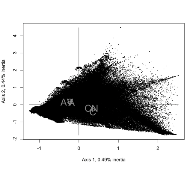
Figure 1: 880664 Twitter tweets projected on the principal factor, i.e. principal axis plane, with attributes projected.

Our first task is to have an analogy of a two-dimensional histogram of what is displayed in the two previous figures. This can be advanced towards an image representation. Pixellation of a spatial domain can be displayed using heatmaps, or false colour coding, implying the predominant visualization role for such display.

2 Algorithm for Determining and Contextual Displaying of a Two-Dimensional Histogram

Pixellating the data is equivalent to hashing, and for an image representation, the viewpoint is employed, of having this considered as a two-dimensional (2D) histogram.

2.1 Pixellating the Mapped Data Point Cloud

Firstly, given that the factor space is endowed with the Euclidean distance, the coordinates of the projected cloud of points can be rescaled. One reason for this is to have a standardized algorithmic processing approach. If there were to be particular topological patterns (e.g. the horseshoe effect, curvilinear pattern related to cluster ordering through embeddedness) or other targeted cluster morphologies (shapes, whether in two dimensions or in the full dimensional space), the the analytics would focus on such patterns. Here, algorithmically, the general and generic objective is carried out by mapping the coordinates of the projected data cloud, in the factor plane, onto coordinates that are in the (closed lower bound, open upper bound) interval $[0,1)$. This mapping results from the interval of minimum value, maximum value, on each coordinate.

This then allows pixellation of the rescaled, unit square area containing the mapped cloud of points. This could be generalized also to unit volumes if more than two factors are at issue. Pixellation, i.e. imposing a regular grid, can be displayed as a grid structure. Furthermore, the pixel value is to be defined by the frequency of occurrence of points mapped into the given pixel area. To be both precise about what is displayed and to be computationally and storage efficient, the frequency of occurrence values, comprising our pixel values here, will be displayed.

Such objectives in data analysis are largely consistent with the computational and interpretational advantages and benefits that are described in [5]. First we may note that the heatmap display, provides colour coding of the data matrix values. This is based on permutation of rows and columns with adjacency that is compatible with the hierarchical clustering of both rows and of columns. Such visualization of hierarchical clustering is at issue in [12].

Now, a similar view of analysis might start with a very large data array and decide that a convenient and computationally efficient analysis process is as follows. Firstly, have the rows and columns permuted so that there is at least some relevance of the proximity taken into account by the permutation. In [5], this was based on principal factor projections. Then, secondly, the row and column permuted input data array is considered such that all array values are the pixel values of an image. So the input data array is thus considered as an image. Then computationally efficient processing can be undertaken on the image representation of the input data array. Such processing is quite likely to involved a wavelet transform of the image, with filtering carried out in wavelet transform space. This provides a manner of determining clusters, and all is very relevant when visualization is an desirable outcome.

In a sense therefore, at issue here, firstly, is the carrying out of the factor space mapping, endowed with the Euclidean metric, and that can be computationally efficient if, for example, having $n$ rows, and $m$ columns, then eigen-reduction that determines the factor space mapping, when $m<<n$, is computationally, $O(m^{3})$. This can be quite efficient, assuming that $m<<n$. Then all of the work here is, analogously, to map large data arrays into images, here directly based on the Euclidean metric endowed factor space.

Sample R code used for pixellation is available at this website,
http://www.multiresolutions.com/strule/papers.

3 Visualization through 2D Histogram Representation

Following Figure 1, Figure 2 shows how we can have displays that are both informative and also that provide alternative display capability for very large numbers of projection locations, i.e. mapped rows or columns, observations and attributes.

In Figure 2, it seems visually that the high frequency value in the grid cell that has a projection greater than 4 on axis 2, and greater than 1 on axis 1, is unacceptably high in value. This grid cell has 13333 projected points. In fact we verified that there are 13333 overlapping points here. (Their values on factor 2 are all: 4.476693).

A heatmap may be derived from this representation, that is grid-based and can be characterized as a 2-dimensional histogram. The heatmap, being false colour coding of the data matrix being hierarchically clustered, in regard to both the row set and the column set, is used in [12]. Such a heatmap display has a somewhat different objective, relative to what will now follow. Our later aim is have the data structured to support search and retrieval.

3.1 Varying Number Theoretic Representations of the Data: m-Ary and p-Adic Representations

Having pixellated the projected cloud of points, this is based on associating each projected point with its grid cell. Integral to this is that the grid cell containing the projected point becomes an expression that labels each of its grid cell members. This is analogous to projected point being a member of a cluster, and perhaps also it is analogous to the projected point being conceptually characterized by the superset of projected points associated with the grid cell. Since the grid cells are defined by default as decimal numbers, that will also be termed here, 10-ary, i.e. m-ary with m = 10, we will next considered alternative number theoretic representations. With p being a prime number, and m being a non-prime integer, we will consider the best fitting grid cell mapping representations that are derived from the decimal or m = 10, m-ary, representation. We considered: m = 9, m = 8, p = 7, m = 6, p = 5, m = 4, p = 3, p = 2, number representations.

Considerable background discussion on p-adic number systems, and their role in various domains, is in [10]. Specifically using the algorithm now to be described, for closest fit of one number theoretic system to another, this is described in [8].

Algorithmically to move from an $m=10$ $m$-ary representation to an $m=9$ $m$-ary representation, we take the definition of the grid cells from their projections on factor 1 and on factor 2. We first consider factor 1, i.e. axis 1, with identical reasoning applied to factor 2, i.e. axis 2. Let $v$ be the constant interval between grid lines. For $m=10$, we have the axis 1 values as follows: $0,0+v,0+2v,0+3v,\dots,0+9v$. We now want to form grid cell boundaries for $m=9$, so that on axis 1, we will have: $0,0+v^{\prime},0+2v^{\prime},0+3v^{\prime},\dots,0+0+8v^{\prime}$.

Because we want a closest fit by the 9-ary representation to the 10-ary representation, the former is based on the latter. We take the least difference between the total sum of successive grid bins. In effect, then, we merge these two successive grid bins. By relabelling higher valued grid bin sequence numbers, this directly provides us with a 9-ary representation.

The same approach is used for factor 2, i.e. axis 2. Then we can proceed through further stages, to find a best fit 8-ary representation to the just determined 9-ary representation. The following stage is to find a best fit 7-ary representation to the just determined 8-ary representation. This continues stagewise until we have a 2-ary representation, i.e. a binary representation of the grid cell axis 1 and axis 2 projections.

Further study of pixellation was for a $9\times 9$ grid display, an $8\times 8$ grid display, a $7\times 7$ grid display, and so, continuing to a $2\times 2$ grid display. The latter is associated with a binary encoding of the grid cell boundary coordinates.

Thus, to state what is at issue here, it is visualization through 2D (two-dimensional) histogram display, possibly accompanying m-adic and p-adic representation, in our mapped or represented data.

We may wish to determine a rather good display of the supplementary elements relative to particular grid cells.

There can be the display of local densities using the projected elements. Taking previous outputs, Figure 3 displays local densities of the tweets, provided by the $10\times 10$ grid. The grid cells can be considered as three dimensional histogram bins. Then in Figure 4, the supplementary variables are projected, relating to the words used for the Cannes Film Festival, and the Avignon Theatre Festival. At issue here is largely the display.

Figure 2: A $10\times 10$ grid display with supplementary elements projected. These projections, associated with tweet content, are related to the Cannes Film festival and the Avignon Theatre festival.

4 Hashing and Binning for Nearest Neighbour Searching

In [4], a framework for all that is at issue here was described with relevance in the fields of information retrieval and kindred areas related to search and retrieval. For nearest neighbour searching, what is discussed initially is: hashing, or simple binning or bucketing. The grid structure cell constitutes the way forward for searching in other neighbours of the query point that have also been mapped into the one grid cell. Some consideration may need to be given to one or more adjacent grid cells if the query point is closer to a grid cell boundary, than it is to any potential nearest neighbour in the given grid cell. With uniformly distributed data, here in the 2-dimensional context, then it is noted how constant time, i.e. $O(1)$ time, is the expectation (statistical first order moment, mean) of the computational time. A proof of this is in [1].

It is to be noted, [4], p. 33, that when searching requires use of adjacent multidimensional grid cells, by design hypercube in their hypervolume, then this implies a computational limitation that increases with dimensionality. In [4], for dimensionality reduction that supports nearest neighbour searching, reference is made to principal components analysis, non-metric multidimensional scaling, and self-organising feature maps. In our work here, Correspondence Analysis provides semantic mapping, i.e. the factor that is, in effect, the principal component space, with a unified scale for both observations and attributes.

Extending this approach to higher dimensional spaces, there is the k-d (k-dimensional, for integer, k) tree, or multidimensional binary search tree. This is a balanced tree, by design, representation of the multidimensional point cloud. Stepwise binarization of the data is carried out using the median projection on each axis. However, the computational complexity of requiring the checking of adjacent clusters that are, by design, hyperrectangular, has the following consequence: computationally such an approach needs to be limited in the dimensionality. Up to dimensionality of 8 is reported on in the literature.

Also discussed in [4] are bounds on the nearest neighbour distance, given a candidate nearest neighbour; other such bounding using metric properties, especially the triangular inequality; branch and bound is the at issue in such methodology; for high dimensional, sparse, binary data, and where binary here represents presence or absence values in, e.g., keyword-based document data (as an example, there could be 10,000 documents, crossed by the presence or absence of 10,000 keywords). For the high dimensional, sparse, binary data, such data has always been traditional in information retrieval, and what is used is the mapping of documents to keywords, and the inverted file that is the mapping of keywords to documents. Cluster-based retrieval can extend some of these approaches. Further discussion in [4] is for range searching using the quadtree, for 2-dimensional images, the octree, for 3-dimensional data cubes (just one example here is a 3-dimensional image volume), and a quadtree implementation on a sphere, for spherical data. The latter is relevant for remotely senses earth data, and for cosmological data. Range searching involves moving beyond location-oriented search.

Figure 3: The grid structure, used for the 2-dimensional histogram binning, is not displayed but the histogram bin values alone.

5 Multidimensional Baire Distance

An open issue, motivated by this work, is to aim at having a multidimensional Baire distance. This could be based on the following. Take a full factor space, perhaps with 5 factors retained (as it the default in the FactoMineR package in R), and for such labels here as C, A, etc., looking at grid binned factor pairwise (biplots) supplementary mapping. This is to to see what grid cells are relevant for the supplementary elements. But, based on this approach, we may have supplementary rows or individuals, that with Twitter data, is to then do digit-wise mapping of tweets against the selected supplementary elements.

In general, related to such a multidimensional Baire distance is the Baire distance formulated for multi-channel data, i.e. hyperspectral images, and used for machine learning (Support Vector Machine, supervised classification) in [3].

6 Conclusion

A central theme of this work can be expressed as follows: performing data mapping that results in a domain-relevant data encoding. One aim of the work here has been to benefit from just how very evident it is, that human visual-based information, and both measure and approximated data, become very efficient as well as effective. At issue are: image, display, biplot. Further practical benefits are demonstrated in [5], by representing the data to be analyzed as an image, and thereby carrying out wavelet transform based filtering, and object detection, and so on.

Informally expressed, therefore, we may state that this work is in relation to the visualization of data, that accompanies having the data verbalized: see [2] for this phrasing. The application objectives cover data mining (as contrasted with supervised classification and mainstream data mining), data analytics (encompassing both processing and output), and inductive reasoning (what the analysis achieves). Furthermore, the computational complexity of the processing and all of the implementation is implicit in this work.

Largely, the terms used here, pixellation and a 2D histogram, are identical. Search in Big Data is the basis for matching, such as in nearest neighbour matching, and associated or relevant data querying. Although not always done, from a mathematical sciences point of view, well-based, past work ought to be cited. In [6], chapter 2 entitled “Fast nearest neighbour searching” covers multidimensional binary search tree structuring of the data, and hashing for nearest neighbour or best match searching, accompanied by implementation optimization, and with twenty two references on these, and directly related, themes.

All that is at issue here is open to the possibility of implementation using distributed computing. While further research will deal with case studies arising and motivated by this work, a further aim will be to have distributed computing implementations also set up and functioning operationally.

Figure 4: As previous figure, Figure 3, with supplementary elements projected. These projections, associated with tweet content, are related to the Cannes Film festival and the Avignon Theatre festival.

References

- [1] Bentley, J.L., Weide, B.W., Yao, A.C.: “Optimal expected time algorithms for closest point problems”, ACM Transactions on Mathematical Software, 6, 563–580 (1980)
- [2] Blasius, J., Greenacre, M. (eds.): Visualization and Verbalization of Data, Chapman and Hall/CRC Press, Boca Raton, Florida (2014)
- [3] Bradley, P.E., Braun, A.C.: “Finding the asymptotically optimal Baire distance for multi-channel data”, Applied Mathematics, 6 (3), 484–495 (2015)
- [4] Murtagh, F.: Search algorithms for numeric and quantitative data, Chapter 4, pp. 29–48, in Heck, A., Murtagh, F. (eds.) Intelligent Information Retrieval: The Case of Astronomy and Related Space Sciences, Kluwer, Dordrecht (1993)
- [5] Murtagh, F., Starck, J.-L., Berry, M.W.: Overcoming the curse of dimensionality in clustering by means of the wavelet transform, Computer Journal, 43(2), 107–120 (2000)
- [6] Murtagh, F.: Multidimensional Clustering Algorithms, Physica-Verlag, Vienna-Würzburg (1985)
- [7] Murtagh, F., Contreras, P.: Random projection towards the Baire metric for high dimensional clustering, in Gammerman, A., Vovk, V., Papadopoulos, H. (eds.) Statistical Learning and Data Sciences, Springer Lecture Notes in Artificial Intelligence (LNAI) Volume 9047, 424–431 (2015)
- [8] Murtagh, F.: Sparse p-Adic Data Coding for Computationally Efficient and Effective Big Data Analytics, p-Adic Numbers, Ultrametric Analysis and Applications, 8(3), 236–247 (2016) https://arxiv.org/abs/1604.06961
- [9] Murtagh, F.: Semantic Mapping: Towards Contextual and Trend Analysis of Behaviours and Practices”, in Balog, K., Cappellato, L., Ferro, N., MacDonald, C. (eds.), Working Notes of CLEF 2016 - Conference and Labs of the Evaluation Forum, Évora, Portugal, 5–8 September, 2016, pp. 1207–1225 (2016) http://ceur-ws.org/Vol-1609/16091207.pdf
- [10] Murtagh, F.: Data Science Foundations: Geometry and Topology of Complex Hierarchic Systems and Big Data Analytics, Chapman and Hall, CRC Press (2017)
- [11] Murtagh, F.: Big data scaling through metric mapping: exploiting the remarkable simplicity of very high dimensional spaces using Correspondence Analysis, in Palumbo, R. et al. (eds.), Data Science, Studies in Classification, Data Analysis, and Knowledge Organization, Springer, pp. 279–290 (2017)
- [12] Zhongheng Zhang, Murtagh, F., Van Poucke, S.: Su Lin, Peng Lan, Hierarchical cluster analysis in clinical research with heterogeneous study population: highlighting its visualization with R, Annals of Translational Medicine, 5(4), (Feb. 2017) http://atm.amegroups.com/article/view/13789/pdf